Spectral properties of graphs associated to the Basilica group

Abstract.

We provide the foundation of the spectral analysis of the Laplacian on the orbital Schreier graphs of the Basilica group, the iterated monodromy group of the quadratic polynomial $z^{2}-1$. This group is an important example in the class of self-similar amenable but not elementary amenable finite automata groups studied by Grigorchuk, Żuk, Šunić, Bartholdi, Virág, Nekrashevych, Kaimanovich, Nagnibeda et al. We prove that the spectrum of the Laplacian has infinitely many gaps and that the support of the KNS Spectral Measure is a Cantor set. Moreover, on a generic blowup, the spectrum coincides with this Cantor set, and is pure point with localized eigenfunctions and eigenvalues located at the endpoints of the gaps.

1. Introduction

The Basilica group is a well studied example of a self-similar automata group. It has interesting algebraic properties, for which we refer to the work of Grigorchuk and Żuk, who introduced the group in [26] and studied some of its spectral properties in [27], and of Bartholdi and Virág [11], who proved that it is amenable but not sub-exponentially amenable. However the spectral properties of the Basilica do not seem to be fully accessible using the techniques introduced in the foundational papers [7, 8]. By work of Nekrashevych [41] the Basilica group is an iterated monodromy group and has as its limit set the Basilica fractal, which is the Julia set of $z^{2}-1$. The resistance form and Laplacian on this fractal were introduced and studied in [44], where it was proved that the spectral dimension $d_{s}$ of the Basilica fractal is equal to $\frac{4}{3}$. In this paper we combine an array of tools from various areas of mathematics to study the spectrum of the orbital Schreier graphs of the Basilica group. Our work is strongly motivated by recent results of Grigorchuk, Lenz, and Nagnibeda, see [23, 22, and references therein].

As for self-similar groups in general, a great deal of the analysis of the Basilica group rests on an understanding the structure of its Schreier graphs and their limits. Many properties of such graphs were obtained by D’Angeli, Donno, Matter and Nagnibeda [14], including a classification of the orbital Schreier graphs, which are limits of finite Schreier graphs in the pointed Gromov-Hausdorff sense. In the present work we consider spectral properties of some graphs obtained by a simple decomposition of the Schreier graphs. These graphs may still be used to analyze most orbital Schreier graphs.

Our main results include construction of a dynamical system for the spectrum of the Laplacian on Schreier graphs that gives an explicit formula for the multiplicity of eigenvalues and a geometric description of the supports of the corresponding eigenfunctions, associated formulas for the proportion of the KNS spectral measure on orbital Schreier graphs that is associated to eigenvalues for each of the finite approximation Schreier graphs, and a proof that the spectra of orbital Schreier graphs contain infinitely many gaps and no intervals. We also show that the Laplacian spectrum for a large class of orbital Schreier graphs is pure point.

The paper is arranged as follows:

• In Section 2 we introduce the Basilica group, its Schreier graphs $\Gamma_{n}$ and their Laplacians. We then make a simple decomposition of $\Gamma_{n}$ to introduce graphs $G_{n}$ which will be more tractable in our later analysis. The main result of Section 2, Theorem 2.3, is that moving from $\Gamma_{n}$ to $G_{n}$ is of little significance for the limiting structures. Specifically we show that, with one exception, all isomorphism classes of orbital Schreier graphs of the Basilica group are also realized as infinite blowups of the graphs $G_{n}$. Conversely, all blowups of $G_{n}$, except those with boundary points, are orbital Schreier graphs of the Basilica group.

• In Section 3 we give a dynamical description of the spectrum of $G_{n}$ which reflects the self-similarity in its construction. It should be noted that a different dynamical system for the spectrum of the Basilica was obtained some time ago in [27] by another method, but we do not know whether it is possible to do our subsequent analysis for that system. Subsection 3.1 introduces our first recursion for characteristic polynomials of the Laplacian. Subsection 3.2 describes localized eigenfunctions and Theorem  3.11 provides a factorization of the characteristic polynomial for the $G_{n}$ Laplacian which separates eigenvalues introduced in earlier levels of the structure and counts their multiplicities using the number of copies of localized and non-localized eigenfunctions. The recusive dynamics of these factors is considered in more detail in subsection 3.3, where we find in Corollary 3.14 that a vastly simpler dynamics is valid for a rational function having roots at the eigenvalues for $G_{n}$ that are not eigenvalues of any earlier $G_{k}$, $k<n$, and poles at the latter values with specified multiplicities. This simpler dynamics is crucial in our later work because it is susceptible to a fairly elementary and direct analysis.

• In Section 4, Theorem 4.6, we prove an approximation result for the Kesten–von-Neuman–Serre (KNS) spectral measure of a blowup $G_{\infty}$ of the graphs $G_{n}$, which is a version of the integrated density of states. For details of this measure we refer to [28].

• In Section 5 we prove the existence of gaps, which are intervals that do not intersect the spectum of the Laplacian for any of the graphs $G_{n}$, and show that for each $\lambda$ in the spectrum of the Laplacian for some $G_{n}$ there is a sequence $k_{j}$ and spectral values for the Laplacian on $G_{n+2k_{j}}$ that accumulate at $\lambda$, see Theorem 5.4. It follows readily that the support of the KNS spectral measure is a Cantor set.

• In Section 6 we use the approach developed in [55, 38] to show that a generic set of blowups of the graphs $G_{n}$, or equivalently a generic set of orbital Schreier graphs, have pure point spectrum, see Theorem 6.4. It follows that the spectrum of the natural Markov operator on the blowup, which is sometimes called the Kesten spectrum, coincides with the Cantor set that forms the support of the KNS spectral measure.

The motivation for our work comes from three sources. First, we are interested to develop methods that provide more information about certain self-similar groups, see the references given above and [34, 33, 32, 42, 10]. Second, we are interested to develop new methods in spectral analysis on fractals. Our work gives one of the first results available in the literature that gives precise information about the spectrum of a graph-directed self-similar structure, making more precise the asymptotic analysis in [29]. For related results in self-similar setting, see [55, 6, 30, 54, 12, 31, 16, 15, 40, 53, 20, 19, 49, 18, 18, 50, 48, 47, 46, 45]. One can hope that spectral analysis of the Laplacian on Schreier graphs in some sense can provide a basis for harmonic analysis on self-similar groups, following ideas of [51, 56]. Third, our motivation comes from the works in physics and probability dealing with various spectral oscillatory phenomena [1, 17, 21, 37, 36, 35, 2, and references therein]. In general terms, our results is a part of the study of the systems with aperiodic order, see [3, 13, 5, 4, and references therein].

Acknowledgments

The last two authors thank Nguyen-Bac Dang, Rostislav Grigorchuk, Mikhail Lyubich, Volodymyr Nekrashevych, Tatiana Smirnova-Nagnibeda, and Zoran Šunić for helpful and interesting discussions.

2. The graphs $\Gamma_{n}$ and $G_{n}$ and their Laplacians

2.1. The Basilica group and its Schreier graphs

Let $T$ be the binary rooted tree. We write its vertices as finite words $v\in\{0,1\}^{*}:=\cup_{n=0}^{\infty}\{0,1\}^{n}$; a vertex $v=v_{1}\dotsm v_{n}$ is said to be of level $n$, and by convention $\{0,1\}^{0}=\emptyset$ is the null word. The edges containing the vertex $v=v_{1}\dotsm v_{n}$ go to the children $v0$, $v1$ and the parent $v_{1}\dotsm v_{n-1}$. Evidently a tree automorphism of $T$ preserves the levels of vertices. The set of right-infinite words, which may be considered to be the boundary of $T$, is written $\{0,1\}^{\omega}=\partial T$.

The Basilica group is generated by an automaton. There is a rich theory of automata and automatic groups, for which we refer to the expositions in [41, 9]. For the Basilica the automaton is a quadruple consisting of a set of states $\mathcal{S}=\{e,a,b\}$ (where $e$ means identity), the alphabet $\{0,1\}$, a transition map $\tau:\mathcal{S}\times\{0,1\}\to\mathcal{S}$ and an output map $\rho:\mathcal{S}\times\{0,1\}\to\{0,1\}$. It is standard to present the automaton using a Moore diagram, given in Figure 1, which is a directed graph with vertex set $\mathcal{S}$ and arrows for each $(s,j)$, $j\in\{0,1\}$ that point from $s$ to $\tau(s,j)$ and are labelled with $j|\rho(s,j)$.

Figure 1. The Moore diagram for the Basilica group automaton.

The automaton defines, for each $s\in\mathcal{S}$, self maps $\mathcal{A}_{s}$ of $\{0,1\}^{*}$ and $\{0,1\}^{\omega}$ (i.e. $T$ and $\partial T$) by reading along the word from the left and altering one letter at a time. Specifically, given a state $s$ and a word $v=v_{1}v_{2}v_{3}\dotsm$ (which may be finite or infinite), the automaton “reads” the letter $v_{1}$, writes $\rho(s,v_{1})$, moves one position to the right and “transitions” to state $\tau(s,v_{1})$, which then reads $v_{2}$, and so forth. Observe that these $\mathcal{A}_{s}$ are tree automorphisms of $T$. The Basilica group is the group of automorphisms of $T$ generated by the $\mathcal{A}_{s}$ with $s\in\mathcal{S}$.

Classically, a Schreier graph of a group $B$ is defined using a generating set $S$ and a subgroup $H$ by taking the vertices to be the left cosets $\{gH:g\in B\}$ and the edges to be of the form $(g,sg)$ for $s\in S$. In the case that $B$ acts transitively on a set $\tilde{T}$ one takes $H$ to be the stabilizer subgroup of an element; this subgroup depends on the element, but the Schreier graphs are isomorphic. Moreover, one may then identify cosets of $H$ with elements of $\tilde{T}$, at which point the Schreier graph can be thought to have vertex set $\tilde{T}$ and edges $\bigl{\{}\{v,sv\}:v\in\tilde{T},s\in S\setminus\{e\}\bigr{\}}$. Note that we remove the identity from $S$ to avoid unnecessary loops.

The Basilica group is transitive on levels of the binary tree $T$, so we may define a Schreier graph for each level by the above construction. Removing the identity from $\mathcal{S}$ we take the generating set to be $S=\{A_{a},A_{b}\}$. More precisely, the $n^{\text{th}}$ Schreier graph $\Gamma_{n}$ of the Basilica group has vertices the words $\{0,1\}^{n}$ and edges between words $w$, $w^{\prime}$ for which $\mathcal{A}_{a}(w)=w^{\prime}$ or $\mathcal{A}_{b}(w)=w^{\prime}$; it is often useful to label the edge with $a$ or $b$ to indicate the associated generator.

The action of $B$ on the boundary $\partial T$ is not transitive, but for each $v\in\partial T$ we may take the Schreier graph defined on the orbit of $v$, which is just that of the subgroup of $B$ that stabilizes $v$. This is called the orbital Schreier graph $\Gamma_{v}$. If the length $n$ truncation of $v$ is denoted $[v]_{n}$ then the sequence of pointed finite Schreier graphs $(\Gamma_{n},[v]_{n})$ converges in the pointed Gromov-Hausdorff topology to $(\Gamma_{v},v)$. One description of this convergence is to define the distance between pointed graphs $(\Gamma^{\prime},x^{\prime}),(\Gamma^{\prime\prime},x^{\prime\prime})$ as follows:

(2.1) $$\operatorname{dist}_{pGH}=\inf\Bigl{\{}\frac{1}{r+1}:B(x^{\prime},r)\text{ is graph isomorphic to }B(x^{\prime\prime},r)\Bigr{\}}.$$

A classification of the orbital Schreier graphs of the Basilica group is one main result of [14].

It is helpful to understand the relationship between the Schreier graphs for different levels. To see it, we compute for a finite word $w$ that $a(1w)=1e(w)=1w$ and $a(0w)=0b(w)$, while $b(1w)=0e(w)=0w$ and $b(0w)=1a(w)$. This says that at any word beginning in $1$ there is an $a$-self-loop and a $b$-edge $\{1w,0w\}$. It also says that if there is a $b$-edge $\{w,b(w)\}$ at scale $n$ then there is an $a$-edge $\{0w,0b(w)\}$ at scale $(n+1)$, if there is an $a$-edge $\{w,a(w)\}$ at scale $n$ there is a $b$-edge $\{0w,1a(w)\}$ at scale $n+1$, and if there is an $a$-loop at $w$ there are two $b$-edges between $0w$ and $1w$. With a little thought one sees that these may be distilled into a set of replacement rules for obtaining $\Gamma_{n+1}$ from $\Gamma_{n}$. Each $b$-edge in $\Gamma_{n}$ becomes an $a$-edge in $\Gamma_{n+1}$, an $a$-loop at $1w$ becomes two $b$-edges between $01w$ and $11w$, and an $a$-edge, which can only be between words $0w,0b(w)$, becomes $b$-edges from $10b(w)$ to both $00w$ and $00b(w)$; $a$-loops are also appended at words beginning in $1$. These replacement rules are summarized in Figure 2 and may be used to construct any $\Gamma_{n}$ iteratively, beginning at with $\Gamma_{1}$, which is shown along with $\Gamma_{2}$ and $\Gamma_{3}$ in Figure 3. For a more detailed discussion of these rules see Proposition 3.1 in [14].

Figure 2. Replacement Rules for $\Gamma_{n}$

Figure 3. The graphs $\Gamma_{1},\Gamma_{2}$ and $\Gamma_{3}$.

2.2. The graphs $G_{n}$

In order to simplify some technicalities in the paper we do not work directly with the graphs $\Gamma_{n}$ but instead treat graphs $G_{n}$ defined as follows. For $n\geq 2$, replace the degree four vertex $0^{n}$ in $\Gamma_{n}$ with four vertices, one for each edge incident upon $0^{n}$, and call these boundary vertices. Observe that this produces two new graphs, each with two boundary vertices. Denote the smaller subgraph by $G_{n-1}$ and observe that the self-similarity of $\Gamma_{n}$ implies the larger subgraph is isomorphic to $G_{n}$. Using the addressing scheme for the finite Schreier graphs, if $n\geq 2$ the subgraph $G_{n-1}$ consists of those vertices in $\Gamma_{n}$ with addresses ending in $10$, plus the boundary vertices. Evidently one can recover the graph $\Gamma_{n}$ by identifying the boundaries of $G_{n}$ and $G_{n-1}$ as a single point; we return to this idea later and illustrate it for $n=3$ in Figure 5. We denote the set of boundary points of $G_{n}$ by $\partial G_{n}$.

Let $G_{0}$ be the complete graph on two vertices, with the edge labelled $a$. We may generate the graphs $G_{n}$ from $G_{0}$ using the same replacement rules for $\Gamma_{n}$ that are depicted in Figure 2. Figure 4 illustrates the first few approximating graphs of $G_{n}$.

Figure 4. Graphs $G_{n}$, $n=0,1,2,3$

We define a Laplacian $L_{n}$ on $G_{n}$ in the usual manner. Let $\ell^{2}_{n}$ denote the functions $\mathbb{R}^{G_{n}}$ with $L^{2}$ norm with respect to counting measure on the vertex set. For vertices $x,y$ of $G_{n}$ let $c_{xy}$ be the number of edges joinng $x$ and $y$ and note that $c_{xy}\in\{0,1,2\}$.

Definition 2.1.

The Laplacian on $\ell^{2}_{n}$ is

(2.2) $$L_{n}f(x)=\sum c_{xy}(f(x)-f(y)).$$

$L_{n}$ is self-adjoint, irreducible because $G_{n}$ is connected, and non-negative definite because $\sum f(x)L_{n}f(x)=\sum c_{xy}(f(x)-f(y))^{2}$.

We will also make substantial use of the Dirichlet Laplacian, which is given by (2.2) but with domain the functions $\mathbb{R}^{G_{n}\setminus\partial G_{n}}$.

2.3. Blowups of $G_{n}$ and their relation to Schreier graphs

Since our graphs $G_{n}$ are not Schreier graphs we cannot take orbital graphs as was done in the Schreier case. A convenient alternative is a variant of the notion of fractal blowup due to Strichartz [52], in which a blowup of a fractal defined by a contractive iterated function system is defined as the union of images under branches of the inverses of the i.f.s. maps. The corresponding idea in our setting is to use branches of the inverses of the graph coverings corresponding to truncation of words; these inverses are naturally represented by appending letters. The fact that we restrict to $G_{n}$ means words with certain endings are omitted.

Recall that in the usual notation for finite Schreier graphs, $G_{n}$, $n\geq 2$, is isomorphic to the subset of $\Gamma_{n}\setminus\{0^{n}\}$ consisting of words that do not end with $10$, except that the vertex $0^{n}$ is replaced with two distinct boundary vertices which we will write $0^{n-1}x$ and $0^{n-1}y$; if $n\geq 3$ the former is connected to a vertex ending in $0$ and the latter to one ending in $1$. One definition of an infinite blowup is as follows.

Definition 2.2.

An infinite blowup of the graphs $G_{n}$ consists of a sequence $\{k_{n}\}_{n\in\mathbb{N}}\subset\mathbb{N}$ with $k_{1}=2$ and $k_{n+1}-k_{n}\in\{1,2\}$ for each $n$, and corresponding graph morphisms $\iota_{k_{n}}:G_{k_{n}}\mapsto G_{k_{n+1}}$ of the following specific type. If $k_{n+1}-k_{n}=1$ then $\iota_{k_{n}}$ is the map that appends $1$ to each non-boundary address and replaces both $x$ and $y$ by $01$. If $k_{n+1}-k_{n}=2$ then $\iota_{k_{n}}$ is one of two maps: either the one that appends $00$ to non-boundary addresses and makes the substitutions $x\mapsto 00x$, $y\mapsto 001$, or the one that appends $01$ to non-boundary addresses and makes the substitutions $x\mapsto 001$ and $y\mapsto 00y$. Now let $G_{\infty}$ be the direct limit (in the category of sets) of the system $(G_{k_{n}},\iota_{k_{n}})$. We write $\tilde{\iota}_{k_{n}}:G_{k_{n}}\to G_{\infty}$ for the corresponding canonical graph morphisms.

Note that the choice $k_{1}=2$ was made only to ensure validity of the notation for $G_{n}$ when definining $\iota_{k_{n}}$; with somewhat more notational work we could begin with $k_{1}=0$.

Theorem 2.3.

With one exception, all isomorphism classes of orbital Schreier graphs of the Basilica group are also realized as infinite blowups of the graphs $G_{n}$. Conversely, all blowups of $G_{n}$ except those with boundary points are orbital Schreier graphs.

Proof.

The orbital Schreier graph $\Gamma_{v}$ associated to the point $v\in\partial\Gamma$ is the pointed Gromov-Hausdorff limit of the sequence $(\Gamma_{k},[v]_{k})$, using the distance in 2.1. Now choose $k_{n}$ with $k_{n+1}-k_{n}\in\{1,2\}$ such that none of the finite truncations $[v]_{k_{n}}$ end in $10$ and hence $[v]_{k_{n+1}}$ is obtained from $[v]_{k_{n}}$ by appending one of $00$, $01$, or $1$. The corresponding maps $\iota_{k_{n}}:G_{k_{n}}\to G_{k_{n+1}}$ define a fractal blowup associated to the boundary point $v$. We immediately observe that if the distance between $[v]_{k_{n}}$ and $0^{k_{n}}$ diverges as $n\to\infty$ then the sequence $(G_{k_{n}},[v]_{k_{n}})$ converges in the pointed Gromov-Hausdorff sense (2.1) to the limit of $(\Gamma_{k_{n}},[v]_{k_{n}})$, which is precisely the orbital Schreier graph $(\Gamma_{v},v)$.

In the alternative circumstance that the distance between $[v]_{k_{n}}$ and $0^{k_{n}}$ remains bounded we determine from Proposition 2.4 of [14] that $v$ is of the form $w\bar{0}$ or $w\bar{01}$, where $w$ is a finite word. Moreover, in this circumstance Theorem 4.1 of [14] establishes that $\Gamma_{v}$ is the unique (up to isomorphism) orbital Schreier graph with 4 ends. Accordingly, our infinite blowups capture all orbital Schreier graphs except the one with 4 ends.

The converse is almost trivial: the definition of an infinite blowup gives a sequence $k_{n}$ and corresponding elements of $\{1,00,01\}$. Appending these inductively defines an infinite word $v$ and thus an orbital Schreier graph. If $v$ is not of the form $w\bar{0}$ or $w\bar{01}$ then the orbital Schreier graph is simply $G_{\infty}$ with distinguished point $v$. Otherwise the blowup is not the same as the orbital Schreier graph for the unsurprising reason that the blowup contains $\bar{0}$ as a boundary point. ∎

2.4. The Laplacian on a blowup

Fix a blowup $G_{\infty}$ given by sequences $k_{n}$ and $\iota_{k_{n}}$ as in Definition 2.2 and let $l^{2}$ denote the space of functions on the vertices of $G_{\infty}$ with counting measure and $L^{2}$ norm.

Definition 2.4.

The Laplacian $L_{\infty}$ on $l^{2}$ is defined as in (2.2) where $c_{xy}$ is the number of edges joining $x$ to $y$ in $G_{\infty}$.

Recall that $l^{2}_{k_{n}}$ is the space of functions $G_{k_{n}}\to\mathbb{R}$ with counting measure on the vertices. Using the cannonical graph morphisms $\tilde{\iota}_{k_{n}}:G_{k_{n}}\to G_{\infty}$ we identify each $l^{2}_{k_{n}}$ with the subspace of $l^{2}$ consisting of functions supported on $\tilde{\iota}_{k_{n}}(G_{k_{n}})$. It is obvious that if $x\in G_{k_{n}}$ is not a boundary point of $G_{k_{n}}$ then the neighbors of $x$ in $G_{k_{n}}$ are in one-to-one correspondence with the vertices neighboring $\tilde{\iota}_{k_{n}}(x)$ in $G_{\infty}$ and therefore

(2.3) $$L_{\infty}f(\tilde{\iota}_{k_{n}}(x))=L_{k_{n}}\bigl{(}f|_{\tilde{\iota}_{k_{n}}(G_{k_{n}})}\bigr{)}(x).$$

2.5. Number of vertices of $G_{n}$

It will be useful later to have an explicit expression for the number of vertices in $G_{n}$. This may readily be computed from the decomposition in Figure 5.

Lemma 2.5.

The number of vertices in $G_{n}$ is given by

$$V_{n}=\dfrac{2^{2+n}+(-1)^{1+n}+9}{6}.$$

Proof.

$G_{n}$ is constructed from a copy of $G_{n-1}$ and two copies of $G_{n-2}$ in which four boundary points are identified to a single vertex $u$, as shown for the case $n=3$ in Figure 5. Thus $V_{n}$ must satisfy the recursion $V_{n}=V_{n-1}+2V_{n-2}-3$ with $V_{0}=2$, $V_{1}=3$. The formula given matches these initial values and satisfies the recursion because

$$6(V_{n-1}+2V_{n-2}-3)$$

$$=9+2\cdot 9+(-1)^{n}+2(-1)^{n-1}+2^{1+n}+2\cdot 2^{n}-18$$

$$=9+(-1)^{1+n}+2^{2+n}$$

so the result follows by induction. ∎

Figure 5. $G_{3}$ constructed from a copy of $G_{2}$ and two of $G_{1}$.

3. Dynamics for the spectrum of $G_{n}$

It is well known that the spectra of Laplacians on self-similar graphs and fractals may often be described using dynamical systems; we refer to [43, 39, 24] for typical examples and constructions of this type in both the physics and mathematics literature. In particular, Grigorchuk and Zuk [27] gave a description of the Laplacian spectra for the graphs $\Gamma_{n}$ using a two-dimensional dynamical system. Their method uses a self-similar group version of the Schur-complement (or Dirichlet-Neumann map) approach. One might describe this approach as performing a reduction at small scales, in that a single step of the dynamical system replaces many small pieces of the graph by equivalent weighted graphs. In the case of $\Gamma_{n}$ one might think of decomposing it into copies of $G_{2}$ and $G_{1}$ and then performing an operation that reduces the former to weighted copies of $G_{1}$ and the latter to weighted copies of $G_{0}$, thus reducing $\Gamma_{n}$ to a weighted version of $\Gamma_{n-1}$. The result is a dynamical system in which the characteristic polynomial of a weighted version of $\Gamma_{n}$ is written as the characteristic polynomial of a weighted version of $\Gamma_{n-1}$, composed with the dynamics that alters the weights. The spectrum is then found as the intersection of the Julia set of the dynamical system with a constraint on the weights. See [27] for details and [25] for a similar method applied in different circumstances.

The approach we take here is different: we decompose at the macroscopic rather than the microscopic scale, splitting $G_{n}$ into a copy of $G_{n-1}$ and two of $G_{n-2}$, and then reasoning about the resulting relations between the characteristic polynomials. The result is that our dynamical map is applied to the characteristic polynomials rather than appearing within a characteristic polynomial. It is not a better method than that of [27] – indeed it seems it may be more complicated to work with – but it gives some insights that may not be as readily available from the more standard approach.

3.1. Characteristic Polynomials

Our approach to analyzing the Laplacian spectrum for $G_{n}$ relies on the decomposition of $G_{n}$ into a copy of $G_{n-1}$ and two copies of $G_{n-2}$ as in Figure 5.

The following elementary lemma relates the characteristic polynomials of matrices under a decomposition of this type. (This lemma is a classical type and is presumably well-known, though we do not know whether this specific formulation appears in the literature.) It is written in terms of modifications of the Laplacian $L_{n}$ on certain subsets of $G_{n}$. For $Z\subset G_{n}$ let us write $L_{n}^{Z}$ for the operator given by (2.2) with domain $\mathbb{R}^{G_{n}\setminus\partial Z}$. The best-known case is $Z=\partial G_{n}$, giving the Dirichlet Laplacian. Of course when $Z$ is empty we have $L_{n}^{Z}=L_{n}$, which is the Neumann Laplacian.

Lemma 3.1.

Let $G$ be a finite graph, $u$ a fixed vertex, and $C(u)$ the set of simple cycles in $G$ containing $u$. Let $L$ the Laplacian matrix of $G$ (defined as in (2.2)) so the diagonal entry $d_{j}=\sum_{k}c_{jk}$ is the degree of the $j$ vertex and the off-diagonal entries are $-c_{jk}$. If $D(\cdot)$ denotes the operation of taking the characteristic polynomial then

(3.1) $$D(L)=(\lambda-d_{u})D(L^{u})-\sum_{v\sim u}c^{2}_{uv}D(L^{uv})+2\sum_{Z\in C(u)}(-1)^{n(Z)-1}\pi(Z)D(L^{Z}),$$

where $n(Z)$ is the number of vertices in $Z$ and $\pi(Z)$ is the product of the edge weights $c_{jk}$ along $Z$.

Proof.

Recall that the determinant of a matrix $M=[m_{jk}]$ may be written as a sum over all permutations of the vertices of $G$ as follows: $\det(M)=\sum_{\sigma}\operatorname{sgn}(\sigma)\prod_{j}m_{j\sigma(j)}$. With $M=\lambda-L$ observe that each product term is non-zero only when the permutation $\sigma$ moves vertices along cycles on the graph. We factor such $\sigma$ as $\sigma=\sigma^{\prime}\sigma^{\prime\prime}$, where $\sigma^{\prime}$ is the permutation on the orbit $Z$ of $u$. Using the Kronecker symbol $\delta_{jk}$ and writing $Z^{c}$ for the complement of $Z$ we write $D(L)$ as

$$\sum_{\sigma^{\prime}}\operatorname{sgn}(\sigma^{\prime})\prod_{j\in Z}\bigl{(}(\lambda-d_{j})\delta_{j\sigma^{\prime}(j)}+c_{j\sigma^{\prime}(j)}\bigr{)}\sum_{\sigma^{\prime\prime}}\prod_{j\in Z^{c}}\bigl{(}(\lambda-d_{j})\delta_{j\sigma^{\prime\prime}(j)}+c_{j\sigma^{\prime\prime}(j)}\bigr{)}$$

For terms with $\sigma(u)=u$ the values of $\sigma^{\prime\prime}$ run over all permutations of the other vertices, so the corresponding term in the determinant sum is the product $(\lambda-d_{u})D(L^{u})$. When $\sigma^{\prime}$ is a transposition $u\mapsto v\mapsto u$ we have $\operatorname{sgn}(\sigma^{\prime})=-1$ and the product along $Z$ is simply $c_{uv}^{2}$, so the corresponding terms have the form $-c^{2}_{uv}D(L^{uv})$.

The remaining possibility is that the orbit of $u$ is a simple cycle $Z$ containing $n(Z)$ vertices. There are then two permutations $\sigma^{\prime}$ that give rise to $Z$; these correspond to the two directions in which the vertices may be moved one position along $Z$. Each has $\operatorname{sgn}(\sigma^{\prime})=(-1)^{n(Z)-1}$, so the corresponding terms in the determinant expansion are as follows

$$\sum_{\sigma^{\prime}}\operatorname{sgn}(\sigma^{\prime})\prod_{j\in V(u)}c_{j\sigma(j)}\sum_{\sigma^{\prime\prime}}\prod_{j\in V(u)^{C}}\bigl{(}(\lambda-d_{j})\delta_{j\sigma(j)}+c_{j\sigma(j)}\bigr{)}$$

$$\quad=\sum_{\sigma^{\prime}}(-1)^{n(Z)-1}\pi(Z)D(L^{Z})$$

$$\quad=2(-1)^{n(Z)-1}\pi(Z)D(L^{Z})$$

Combining these terms gives (3.1). ∎

In our application of this lemma the important choices of $Z$ are shown in Figure 6, where the corresponding graphs are denoted $A_{n}$, $B_{n}$, $C_{n}$. It will be convenient to write $a_{n}(\lambda)$, $b_{n}(\lambda)$, $c_{n}(\lambda)$ for their respective characteristic polynomials. Note that then the roots of $a_{n}(\lambda)$ are the eigenvalues of the Neumann Laplacian and the roots of $c_{n}(\lambda)$ are the eigenvalues of the Dirichlet Laplacian on $G_{n}$. Our initial goal is to describe these polynomials using a dynamical system constructed from the decomposition in Figure 5.

Figure 6. Graphs $A_{3}$, $B_{3}$, $C_{3}$. Rows and columns corresponding to grey vertices are deleted in the corresponding matrices.

Proposition 3.2.

For $n\geq 4$ the characteristic polynomials $a_{n}$, $b_{n}$ and $c_{n}$ of the graphs $A_{n}$, $B_{n}$ and $C_{n}$ satisfy

$$a_{n} =\bigl{(}2b_{n-1}-3\lambda c_{n-1}-2g_{n-1}\bigr{)}b_{n-2}^{2}+2a_{n-2}b_{n-2}c_{n-1}$$

$$b_{n} =\bigl{(}2b_{n-1}-3\lambda c_{n-1}-2g_{n-1}\bigr{)}b_{n-2}c_{n-2}+(a_{n-2}c_{n-2}+b_{n-2}^{2})c_{n-1}$$

$$c_{n} =\bigl{(}2b_{n-1}-3\lambda c_{n-1}-2g_{n-1}\bigr{)}c_{n-2}^{2}+2b_{n-2}c_{n-2}c_{n-1}$$

where

(3.2) $$g_{n-1}=\prod_{1\leq j<\frac{n}{2}}\bigl{(}c_{n-2j}\bigr{)}^{2^{j-1}}$$

Proof.

Figure 5 illustrates the fact that $G_{n}$ can be obtained from one copy of $G_{n-1}$ and two copies of $G_{n-2}$ by identifying the two boundary vertices of $G_{n-1}$ and one boundary vertex from each of copy of $G_{n-2}$ into a single vertex which we denote by $u$. We apply Lemma 3.1 to $L^{(n)}$ on $G_{n}$ with vertex $u$ to compute the characteristic polynomial. This involves modifying the Laplacian matrix on various sets of vertices. The subgraphs with modified vertices are $A_{n}$, $B_{n}$, and $C_{n}$ as in Figure 6 and also $D_{n}$, $E_{n}$ as in Figure 7.

Figure 7. Graphs $D_{3}$ and $E_{3}$. Rows and columns corresponding to shaded vertices are deleted in the corresponding matrices.

For $n\geq 4$ the point $u$ has one neighbor in each copy of $G_{n-2}$ and two neighbors in the copy of $G_{n-1}$ that lie on a simple cycle which was formed by identifying the boundary vertices. Accordingly the vertex modifications involved in applying Lemma 3.1 are as follows.

Modifying $A_{n}$ at $u$ gives the disjoint union of two copies of $B_{n-2}$ and one of $C_{n-1}$. To modify on $\{u,v\}$ observe that if $v$ is on one of the two copies of $G_{n-2}$ then the result is one copy of each of $B_{n-2}$, $E_{n-2}$ and $C_{n-1}$, while if $v$ is on the copy of $G_{n-1}$ then we see two copies of $B_{n-2}$ and one of $D_{n-1}$. The most interesting modification is that for the cycle. Modifying at $u$ turns the two copies of $G_{n-2}$ into two copies of $B_{n-2}$. The rest of the cycle runs along the shortest path in $G_{n-1}$ between the boundary points that were identified at $u$. Modifying along this causes $G_{n-1}$ to decompose into the disjoint union of one, central, copy of $C_{n-2}$, two copies of $C_{n-4}$ equally spaced on either side and, inductively, $2^{j-1}$ copies of $C_{n-2j}$ for each $j$ such that $2j<n$, equally spaced between those obtained at the previous step. There are also loops along this path which now have no vertices and therefore each have characteristic polynomial $1$. The characteristic polynomial of this collection of $C_{n-2j}$ graphs is $g_{n-1}$.

If we write $d_{n}$ and $e_{n}$ for the characteristic polynomials of $D_{n}$ and $E_{n}$ respectively, then from the above reasoning we conclude that

(3.3) $$a_{n}=(\lambda-4)b_{n-2}^{2}c_{n-1}-2b_{n-2}e_{n-2}c_{n-1}-2b_{n-2}^{2}d_{n-1}-2b_{n-2}^{2}g_{n-1}.$$

Similar arguments beginning with $B_{n}$ or $C_{n}$ instead of $A_{n}$ allow us to verify that

$$b_{n} =(\lambda-4)b_{n-2}c_{n-2}c_{n-1}-b_{n-2}d_{n-2}c_{n-1}-c_{n-2}e_{n-2}c_{n-1}$$

(3.4) $$\quad-2b_{n-2}c_{n-2}d_{n-1}-2b_{n-2}c_{n-2}g_{n-1},$$

$$c_{n} =(\lambda-4)c_{n-2}^{2}c_{n-1}-2c_{n-2}d_{n-2}c_{n-1}-2c_{n-2}^{2}d_{n-1}-2c_{n-2}^{2}g_{n-1}.$$

Another use of Lemma 3.1 allows us to relate some of our modified graphs to one another by performing one additional vertex modification. For example, for $n\geq 3$ we get $C_{n}$ from $B_{n}$ by modifying at one boundary vertex, and this vertex does not lie on a cycle. Deleting the corresponding neighbor gives $D_{n}$, so we must have $b_{n}=(\lambda-1)c_{n}-d_{n}$. In like manner we obtain $a_{n}=(\lambda-1)b_{n}-e_{n}$. These can be used to eliminate $d_{n}$ and $e_{n}$ from equations (3.3) and (3.4) and obtain the desired conclusion. ∎

The initial polynomials $a_{n}$, $b_{n}$, $c_{n}$ for the recursion in Proposition 3.2 are those with $0\leq n\leq 3$. It is fairly easy to compute them for $n=0,1$ directly from the Laplacians of the graphs in Figure 6.

$$a_{0} =\lambda(\lambda-2) b_{0}=\lambda-1 c_{0}=1$$

(3.5) $$a_{1} =\lambda(\lambda-1)(\lambda-3) b_{1}=\lambda^{2}-3\lambda+1 c_{1}=\lambda-2$$

For $n=2,3$ we can use a variant of the argument in the proof of Proposition 3.2, taking the initial graph and modifying the connecting vertex $u$ using Lemma 3.1. In these cases there is no simple cycle, so we need only consider the self-interaction term and the terms corresponding to neighbors, of which there are three: one in the copy of $G_{n-1}$ which is connected by a double edge, so $c^{2}_{uv}=4$, and one in each of the copies of $G_{n-2}$.

For $A_{2}$ modifying $u$ gives a copy of $C_{1}$ and two of $B_{0}$. Additionally modifying a neighbor in one of the two $G_{0}$ copies produces a $C_{0}$, a $B_{0}$ and a $C_{1}$, while deleting the neighbor in the copy of $G_{1}$ decomposes the whole graph into two $B_{0}$ copies and three $C_{0}$ copies. Since $c_{0}=1$ we suppress it in what follows. From this we have an equation for $a_{2}$. Similar reasoning, noting that $u$ has fewer neighbors in $B_{2}$ and $C_{2}$, gives results for $b_{2}$ and $c_{2}$. We summarize them as

$$a_{2} =(\lambda-4)b_{0}^{2}c_{1}-2b_{0}c_{1}-4b_{0}^{2}=\lambda(\lambda^{3}-8\lambda^{2}+15\lambda-8),$$

(3.6) $$b_{2} =(\lambda-4)b_{0}c_{1}-c_{1}-4b_{0}=\lambda^{3}-7\lambda^{2}+9\lambda-2,$$

$$c_{2} =(\lambda-4)c_{1}-4=\lambda^{2}-6\lambda+4.$$

For $A_{3}$ things are more like they were in Proposition 3.2. Modifying at $u$ gives $C_{2}$ and two copies of $B_{1}$, additionally modifying at a neighbor in the $G_{1}$ copies gives a $C_{2}$, $B_{1}$ and $D_{1}$, but $D_{1}=B_{0}$. Modifying at $u$ and the neighbor in the $G_{2}$ copy gives a $C_{1}$ and two copies of $B_{1}$. Reasoning in the same manner for $B_{3}$ and $C_{3}$ we have

$$a_{3} =(\lambda-4)b_{1}^{2}c_{2}-2b_{1}c_{2}d_{1}-4b_{1}^{2}c_{1}$$

$$=\lambda(\lambda-2)(\lambda^{2}-3\lambda+1)(\lambda^{3}-11\lambda^{2}+31\lambda-14)$$

(3.7) $$b_{3} =(\lambda-4)b_{1}c_{1}c_{2}-b_{1}c_{2}-b_{0}c_{1}c_{2}-4b_{1}c_{1}^{2}$$

$$=\lambda^{6}-15\lambda^{5}+79\lambda^{4}-182\lambda^{3}+181\lambda^{2}-62\lambda+4$$

$$c_{3} =(\lambda-4)c_{1}^{2}c_{2}-2c_{1}c_{2}-4c_{1}^{3}$$

$$=(\lambda-2)(\lambda^{4}-12\lambda^{3}+42\lambda^{2}-44\lambda+8)$$

Proposition 3.3.

The characteristic polynomials $a_{n}$, $b_{n}$ and $c_{n}$ may be obtained from the initial data (3.5),(3.6),(3.7), using the following recursions, where we note that that for $c_{n}$ involves only $c$ terms (because the $g_{n}$ are products of $c_{k}$ terms, see (3.2)), that for $b_{n}$ involves only $b$ and $c$ terms, and that for $a_{n}$ involves all three sequences.

(3.8) $$\frac{c_{n}}{c_{n-2}}=\Bigl{(}\frac{c_{n-1}}{c_{n-3}}\Bigr{)}^{2}+2c_{n-1}g_{n-2}-4c_{n-2}g_{n-1},$$

(3.9) $$b_{2m}=c_{2m}\Bigl{(}b_{0}-\sum_{1}^{m}\frac{g_{2j}}{c_{2j}}\Bigr{)},\qquad b_{2m+1}=c_{2m+1}\Bigl{(}b_{1}-\sum_{1}^{m}\frac{g_{2j+1}}{c_{2j+1}}\Bigr{)}$$

(3.10) $$a_{n}c_{n}=b_{n}^{2}-g_{n}^{2}.$$

Proof.

Multiplying the $a_{n}$ equation in Proposition 3.2 by $c_{n-2}^{2}$, the $b_{n}$ one by $-2b_{n-2}c_{n-2}$ and the $c_{n}$ one by $b_{n-2}^{2}$ and summing the results gives the following relationship for $n\geq 4$

$$a_{n}c_{n-2}^{2}-2b_{n}b_{n-2}c_{n-2}+c_{n}b_{n-2}^{2}=0.$$

which can also be verified for $n=2,3$ from (3.5),(3.6), and (3.7). We use it to eliminate $a_{n-2}$ from the equation for $b_{n}$ and thereby obtain recursions for $b_{n}$ and $c_{n}$ that do not involve the sequence $a_{n}$. It is convenient to do so by computing (in the case that $c_{n-2}\neq 0$)

$$a_{n}c_{n}-b_{n}^{2} =\frac{1}{c_{n-2}^{2}}\bigl{(}2b_{n}c_{n}b_{n-2}c_{n-2}-c_{n}^{2}b_{n-2}^{2}-b_{n}^{2}c_{n-2}^{2}\bigr{)}$$

(3.11) $$=\frac{-(b_{n}c_{n-2}-b_{n-2}c_{n})^{2}}{c_{n-2}^{2}}\quad\text{when $n\geq 2$},$$

because we may now compute from Proposition 3.2 and substitute from (3.11) with $n$ replaced by $n-2$ to obtain for $n\geq 4$

$$b_{n}c_{n-2}-c_{n}b_{n-2} =c_{n-1}\bigl{(}a_{n-2}c_{n-2}^{2}+b_{n-2}^{2}c_{n-2}-2b_{n-2}^{2}c_{n-2}\bigr{)}$$

$$=c_{n-2}c_{n-1}\bigl{(}a_{n-2}c_{n-2}-b_{n-2}^{2}\bigr{)}$$

$$=\frac{-c_{n-2}c_{n-1}(b_{n-2}c_{n-4}-b_{n-4}c_{n-2})^{2}}{c_{n-4}^{2}}$$

We can use this to get

$$b_{n}-\frac{c_{n}}{c_{n-2}}b_{n-2}=-c_{n-1}c_{n-3}^{2}c_{n-5}^{4}\dotsm\begin{cases}c_{3}^{2^{(n-4)/2}}(b_{2}-c_{2}b_{0})^{2^{(n-2)/2}}&\text{ if $n$ is even}\\ c_{4}^{2^{(n-5)/2}}(b_{3}-c_{3}b_{1}/c_{1})^{2^{(n-3)/2}}&\text{ if $n$ is odd}\end{cases}$$

however one may compute directly from (3.5) and (3.6) that $b_{2}-c_{2}b_{0}=-c_{1}$ and $b_{3}-c_{3}b_{1}/c_{1}=-c_{2}$, so that for $n\geq 2$

(3.12) $$b_{n}-\frac{c_{n}}{c_{n-2}}b_{n-2}=-g_{n}$$

from which we obtain the expressions in (3.9) by summation and (3.10) by substitution into (3.11).

We may also use this to elminate $b_{n}$ from the expression for $c_{n}$ in Proposition 3.2. A convenient way to do so is to rewrite the equation for $c_{n}$ as

(3.13) $$\frac{c_{n}}{c_{n-1}c_{n-2}^{2}}=2\Bigl{(}\frac{b_{n-1}}{c_{n-1}}+\frac{b_{n-2}}{c_{n-2}}-\frac{g_{n-1}}{c_{n-1}}\Bigr{)}-3\lambda$$

and use (3.12) to eliminate the $b_{n-1}/c_{n-1}$ term. Comparing the result with (3.13) for the case $n-1$ we have both

$$\frac{c_{n}}{c_{n-1}c_{n-2}^{2}} =2\Bigl{(}\frac{b_{n-2}}{c_{n-2}}+\frac{b_{n-3}}{c_{n-3}}-\frac{2g_{n-1}}{c_{n-1}}\Bigr{)}-3\lambda$$

$$\frac{c_{n-1}}{c_{n-2}c_{n-3}^{2}} =2\Bigl{(}\frac{b_{n-2}}{c_{n-2}}+\frac{b_{n-3}}{c_{n-3}}-\frac{g_{n-2}}{c_{n-2}}\Bigr{)}-3\lambda$$

the difference of which is

$$\frac{c_{n}}{c_{n-1}c_{n-2}^{2}}-\frac{c_{n-1}}{c_{n-2}c_{n-3}^{2}}=2\frac{g_{n-2}}{c_{n-2}}-4\frac{g_{n-1}}{c_{n-1}}$$

and may be rearranged to give (3.8) ∎

3.2. Localized Eigenfunctions and factorization of characteristic polynomials.

In this section all eigenfunctions and eigenvalues are Dirichlet, however we will deal extensively with eigenfunctions that satisfy both Dirichlet and Neumann boundary conditions. For convenience we refer to these as Dirichlet-Neumann eigenfunctions.

The principal observation which motivates the results in this section is a set of simple constructions using a symmetry of the graphs $G_{n}$. Recall that $G_{n}$ consists of two copies of $G_{n-2}$, with one boundary vertex from each identified at a point $u$, a copy of $G_{n-1}$ with both boundary vertices identified to $u$, see Figure 5. Let $\Phi_{n}$ denote the graph isometry of $G_{n}$ which reflects in the vertical line of symmetry through the gluing vertex $u$. Thus, $\Phi_{n}$ exchanges the two copies of $G_{n-2}$ and has restriction $\Phi_{n-1}$ to the copy of $G_{n-1}$.

Proposition 3.4.

Dirichlet-Neumann eigenfunctions on $G_{n}$ may be constructed by:

1. Copying a Dirichlet-Neumann eigenfunction for $G_{n-2}$ to either copy of $G_{n-2}$ in $G_{n}$ and extending by zero on the rest of $G_{n}$. The associated eigenvalue has twice the multiplicity in $G_{n}$ that it had in $G_{n-2}$.

2. Copying a Dirichlet-Neumann eigenfunction on $G_{n-1}$ to the copy of $G_{n-1}$ in $G_{n}$ and extending by zero on the rest of $G_{n}$.

3. Copying an eigenfunction on $G_{n-1}$ that is Dirichlet but not Neumann and is antisymmetric under $\Phi_{n-1}$ to the copy of $G_{n-1}$ in $G_{n}$ and extending by zero to the rest of $G_{n}$.

An eigenfunction on $G_{n}$ that is Dirichlet but not Neumann, may be constructed from any eigenfunction on $G_{n-2}$ that is Dirichlet but not Neumann by antisymmetrizing under $\Phi_{n}$ and extending to be zero on the copy of $G_{n-1}$. All eigenfunctions that are $\Phi_{n}$ antisymmetric and Dirichlet but not Neumann are constructed in this manner.

Proof.

We call the constructed function $f$. For all of the constructions the validity of the eigenfunction equation is trivial at all points except the gluing point $u$ where both boundary points of the copy of $G_{n-1}$ and one from each copy of $G_{n-2}$ are identified. Moreover at $u$ we have $f(u)=0$ because all eigenfunctions are Dirichlet. The eigenvalue is the same as that for the functions used in the construction but otherwise plays no role.

To verify that the constructions give eigenfunctions we need only check that $\Delta f(u)=0$. We ignore components on which $f\equiv 0$ as they make no contribution. In the first construction the one non-trivial edge difference at $u$ is zero by the Neumann condition; note that the statement about multiplicities follows from the fact that copies on distinct $G_{n-2}$ sets are independent. In the second construction the Neumann condition ensures the difference on both edges from $u$ into the $G_{n-1}$ set are zero. In the third the differences on these edges are non-zero but opposite in sign because of the asymmetry under $\Phi_{n-1}$. In the fourth the differences are non-zero but opposite in sign because of the antisymmetry under $\Phi_{n}$, and the fact that the restriction of any antisymmetric Dirichlet but not Neumann eigenfunction to each $G_{n-2}$ is a Dirichlet but not Neumann eigenfunction on $G_{n-2}$ establishes the last statement. ∎

Combining the first construction of Dirichlet-Neumann eigenfunctions with the antisymmetric eigenfunction construction yields the following result.

Corollary 3.5.

$c_{k}|c_{n}$ if $k\leq n-2$

In view of the corollary it is natural to factor the $c_{n}$ according to earlier polynomials $c_{k}$.

Definition 3.6.

Let $\gamma_{0}=c_{0}=1$ and inductively set $\gamma_{n}$ to be coprime to $\gamma_{k}$ for each $k<n$ and such that $c_{n}$ is a product of the form

$$c_{n}=\gamma_{n}\prod_{k=1}^{n-1}\gamma_{k}^{s_{n,k}}.$$

We may compute the multiplicities $s_{n,k}$ recursively, but to do so we need to know more properties of the eigenvalues and eigenfunctions that come from each of the factors $\gamma_{k}$.

Proposition 3.7.

If $\lambda$ is a root of $\gamma_{n}$ with eigenfunction $f$ then $f$ is symmetric under $\Phi_{n}$ and non-zero at the gluing point $u$, it has no two adjacent zeros, and it is not Neumann. $\lambda$ is a simple root.

Proof.

If $f(u)=0$ then the restriction to one of the components of $G_{n}\setminus\{u\}$ is not identically vanishing and thus defines an eigenfunction on either $G_{n-2}$ or $G_{n-1}$. This implies $\lambda$ is a root of $c_{m}$ for some $m<n$ in contradiction to the definition of $\gamma_{n}$ as coprime to all such $c_{m}$. Equivalently, if $f$ satisfies the eigenfunction equation with eigenvalue $\lambda$ and $f(u)=0$ then $f\equiv 0$. Now we can antisymmetrize $f$ under $\Phi_{n}$ to get a function satisfying the eigenfunction equation but vanishing at $u$, whence it is identically zero and $f$ was symmetric under $\Phi_{n}$.

Suppose $f(x)=0$. If there is no decoration at $x$ then there are just two edges and a loop meeting at $x$. We call the neighbors $y$ and $y^{\prime}$ and observe that the eigenfunction equation implies $f(y)=-f(y^{\prime})$. If there is a decoration at $x$ then the restriction of $f$ to the decoration must be identically zero or an eigenfunction on $G_{m}$. However we have seen that $\lambda$ cannot be a root of $c_{m}$ for any $m<n$, so $f$ must be identically zero on the decoration. It follows that again $f(y)=-f(y^{\prime})$, where now $y$ and $y^{\prime}$ are the neighbors not in the decoration. Now suppose $f$ is zero at the adjacent points $x$ and $y$. The above reasoning implies $f(y^{\prime})=0$. But then we may work along the graph, each time using the fact that $f$ vanishes at two adjacent points to determine that it vanishes at any attached decorations and at the next adjacent point, and conclude that $f\equiv 0$ in contradiction to the assumption it was an eigenfunction.

Since $f$ is Dirichlet and there is only a single edge attached to each boundary point, if the Neumann condition held at a boundary point then we would have zeros at two adjacent points and could apply the preceding argument. Finally, if there were two eigenfunctions for the same eigenvalue $\lambda$ then a linear combination of them would satisfy the Neumann condition at a boundary point; this contradiction implies $\lambda$ is a simple root. ∎

Lemma 3.8.

Suppose $f$ is an eigenfunction on $G_{n}$ with eigenvalue $\lambda$ which is a root of $\gamma_{m}$. Let $g$ be the unique eigenfunction on $G_{m}$ with eigenvalue $\lambda$ and value $1$ at the gluing point of $G_{m}$. Then the restriction of $f$ to each copy of $G_{m}$ in $G_{n}$ is a multiple of $g$ and the multiples on any two copies of $G_{m}$ that share a boundary point are equal in magnitude and opposite in sign.

Proof.

Decompose $G_{n}$ recursively, subdividing each $G_{k}$ with $k>m$ so that the result is copies of $G_{m}$ and $G_{m-1}$. In Proposition 3.7 we saw that $g$ is symmetric under $\Phi_{m}$ and is not Neumann. On each copy of $G_{m}$ in our decomposition we may subtract a multiple of $g$ such that the resulting function $h$ is zero at the gluing point of each $G_{m}$. Our main goal is to show $h\equiv 0$.

We note two facts which will form the base case of an induction. One is the trivial statement that if $h$ vanishes at both boundary points of copy of $G_{m-2}$ in $G_{n}$ then $h\equiv 0$ on this copy of $G_{m-2}$, simply because $\lambda$ is not a Dirichlet eigenvalue on $G_{m-2}$. The second observation is similar but slightly more complicated: $h\equiv 0$ on any copy of $G_{m-1}$ that is a decoration. The reason is that such a decoration has its boundary points identified at the gluing point of a copy of $G_{m}$; $h$ vanishes at this point by construction, so $h$ satisfies the Dirichlet eigenfunction equation on this $G_{m-1}$, and since $\lambda$ is not a Dirichlet eigenvalue on $G_{m-1}$ it must be that $h\equiv 0$ there.

The induction proceeds by assuming for all $j\leq k$ that $h=0$ on the boundary of a copy of $G_{j-2}$ implies $h\equiv 0$ on this copy, and that $h\equiv 0$ on all decorations that are copies of $G_{j-1}$. We have established the base case $k=m$. One part of the induction is easy. For $j=k+1$, suppose we have a copy of $G_{j-2}=G_{k-1}$ such that $h=0$ on the boundary. Then we may subdivide it as the union of two copies of $G_{k-3}$ and a decorating copy of $G_{k-2}$, glued at $u$. The inductive assumption implies $h\equiv 0$ on the decoration and hence at $u$. Each copy of $G_{k-3}$ has boundary points $u$ and a point from the boundary of the original $G_{k-1}$, so $h=0$ at these points and the inductive hypothesis says $h\equiv 0$ on these copies of $G_{k-3}$. Hence $h=0$ at the boundary of $G_{k-1}$ implies $h\equiv 0$ on $G_{k-1}$.

For the other part of the induction, consider a decoration which is a copy of $G_{k}$ and decompose it into two copies of $G_{k-2}$ and a $G_{k-1}$ decoration, glued at $u$. The induction says $h\equiv 0$ on the decoration, so $h(u)=0$. Moreover, the eigenfunction equation at $u$ says $h(y)=-h(y^{\prime})$, where $y$ and $y^{\prime}$ are the neighbors of $u$, one in each copy of $G_{k-2}$. Symmetrizing $h$ on $G_{k}$ using $\Phi_{k}$ to obtain a function $\tilde{h}$ the preceding says that $\tilde{h}$ vanishes at the boundary point $u$ of both copies of $G_{k-2}$, and at the neighbor of this boundary point. We can therefore run the argument of Proposition 3.7 to find that $\tilde{h}$ is zero on both copies of $G_{k-2}$, where the key fact is that $h$ and thus $\tilde{h}$ vanishes on all decorations of these $G_{k-2}$ by our inductive assumption (in the proof of the lemma the vanishing on decorations was obtained differently). We have shown $\tilde{h}\equiv 0$ on all of the $G_{k}$, so $h$ must have been antisymmetric under $\Phi_{k}$. But $G_{k}$ was assumed to be a decoration, so it has only one boundary point and must therefore vanish at this point. However we have then shown $h=0$ at both boundary points of the copies of $G_{k-2}$, because one of these is the boundary point of $G_{k}$ and the other is $u$, so our inductive assumption implies $h\equiv 0$ on these copies of $G_{k-2}$ and we finally conclude that $h\equiv 0$ on $G_{k}$, completing the induction.

Now the induction allows us to conclude that $h\equiv 0$ on $G_{n}$ because $h=f=0$ on the boundary of $G_{n}$ and $n\geq m$. Thus in our decomposition into copies of $G_{m}$ and $G_{m-1}$ the restriction of $f$ to each copy of $G_{m}$ is a multiple of $g$ and $f$ is identically zero on all copies of $G_{m-1}$. We may then consider the eigenfunction equation at a common boundary point of two copies of $G_{m}$. Since $f$ vanishes on the copies of $G_{m-1}$ the only contributions to the Laplacian are from the edges into $G_{m}$; the eigenfunction equation says they must sum to zero (because this is the value of $f$) and we conclude from this and the symmetry of $g$ on $G_{m}$ that the factors multiplying $g$ on each copy are equal and opposite. ∎

Corollary 3.9.

Suppose $f$ is a Dirichlet eigenfunction on $G_{n}$ that is not also Neumann. If $f$ is symmetric under $\Phi_{n}$ then then the corresponding eigenvalue $\lambda$ is a root of $\gamma_{n}$. If $f$ is antisymmetric under $\Phi_{n}$ then $\lambda$ is a root of $\gamma_{m}$ for some $m$ with $n-m\in 2\mathbb{Z}$ and for each such root there is exactly one eigenfunction (up to scalar multiples) that is not Neumann.

Proof.

By definition of the $\gamma_{m}$ functions, $\lambda$ is a root of exactly one $\gamma_{m}$, $m\leq n$. Suppose it is a root of $\gamma_{m}$ for some $1\leq m<n$ and let $g$ be the unique eigenfunction on $G_{m}$ corresponding to $\lambda$. The previous lemma says that if we decompose $G_{n}$ into copies of $G_{m}$ and $G_{m-1}$ then the restriction of $f$ to each $G_{m}$ copy is a multiple of $g$ and the restriction to each $G_{m-1}$ is identically zero. It is easy to see that if $n-m$ were an odd number then the boundary points would fall in copies of $G_{m-1}$ in this decomposition, but then $f\equiv 0$ in a neighborhood of the boundary would imply $f$ is Neumann, in contradiction to our assumption.

Thus $n-m$ is even and the boundary points fall in copies of $G_{m}$. Note too that there is then a sequence of copies of $G_{m}$ joining the boundary points of $G_{n}$ in the sense that each one has a common boundary point with its predecessor. There are an even number of copies of $G_{m}$ in this sequence, and it is mapped to itself by $\Phi_{n}$. The fact that $f$ is not Neumann means that there is a non-zero multiple of $g$ at each boundary point. Returning to Lemma 3.8 we note that the signs of the multiples of $g$ along our sequence of copies of $G_{m}$ are alternating, so $f$ is antisymmetric under $\Phi_{m}$. There is only one non-Neumann eigenfunction of this type because antisymmetry and the fact there are only two boundary points ensures that for any two there is a linear combination that is Neumann.

We saw that if $\lambda$ is a root of $\gamma_{m}$ for some $m<n$ then $f$ is antisymmetric under $\Phi_{n}$. Hence if $f$ is $\Phi_{n}$ symmetric it must be that $\lambda$ is a root of $\gamma_{n}$. ∎

We also obtain a converse to the part of Proposition 3.4 that concerns construction of Dirichlet-Neumann eigenfunctions.

Corollary 3.10.

All Dirichlet-Neumann eigenfunctions on $G_{n}$ are in the span of those obtained using the constructions (1)–(3) of Proposition 3.4.

Proof.

If the antisymmetrization under $\Phi_{n}$ is not identically zero then the fact that it vanishes at the gluing point of $G_{n}$ implies the restriction to the copy of $G_{n-1}$ is a Dirichlet eigenfunction and so is the restriction to each copy of $G_{n-2}$. Since the restriction of $\Phi_{n}$ to $G_{n-1}$ is $\Phi_{n-1}$ the piece on the copy of $G_{n-1}$ is $\Phi_{n-1}$ antisymmetric and is thus a linear combination of the type constructed in (2) of Proposition 3.4 if this restriction is Neumann and is otherwise of the type constructed in (3). Now consider the restriction to a copy of $G_{n-2}$. It has the Neumann condition at one end; if it also does so at the other then it is as in construction (1) from Proposition 3.4. If not then the symmetrization with respect to $\Phi_{n-2}$ is not Neumann, but Corollary 3.9 then implies its eigenvalue is a root of $\gamma_{n-2}$ and Lemma 3.7 says the corresponding eigenspace is one-dimensional eigenspace and does not contain a function that has a Neumann condition at one end, a contradiction. Thus the antisymmetrization of $f$ under $\Phi_{n}$ is a linear combination of the functions constructed in Proposition 3.4.

Now consider the symmetrization of $f$ under $\Phi_{n}$. In light of Corollary 3.10 and Proposition 3.7 its eigenvalue must be a root of $\gamma_{m}$ for some $m<n$. Decomposing $G_{n}$ into copies of $G_{m}$ and $G_{m-1}$ we find from Lemma 3.8 that its restriction to each copy of $G_{m}$ in $G_{n}$ is a multiple of $g$, the unique corresponding eigenfunction on $G_{m}$, and it vanishes on the copies of $G_{m-1}$. Moreover the factors multiplying $g$ are of equal magnitude and opposite sign on any pair of copies of $G_{m}$ that intersect at a point. We consider two cases.

Case 1: If the boundary points of $G_{n}$ are in copies of $G_{m-1}$ then so is the shortest path between them, which passes through the gluing point. In this case $f$ vanishes all along this path so on both copies of $G_{n-2}$ its restriction is Dirichlet-Neumann, which is consistent with construction (1) from Proposition 3.4. The vanishing at the gluing point also implies the restriction of $f$ to the copy of $G_{n-1}$ is Dirichlet, and the eigenfunction equation at the gluing point forces the sum on the edges from the gluing point into the copy of $G_{n-1}$ to be zero. Thus the part of this restriction which is symmetric under $\Phi_{n-1}$ is Dirichlet-Neumann and comes frm construction (2) of Proposition 3.4, while the antisymmetric part comes from construction (3).

Case 2: If the boundary points of $G_{n}$ are in copies of $G_{m}$ then the fact that $g$ is not Neumann ensures the multiple of $g$ on the copy of $G_{m}$ containing the boundary point is zero. Tracing the alternating signs of these copies along the shortest path between the boundary points we find that $f$ vanishes identically here, so its restriction on both copies of $G_{n-2}$ its restriction is Dirichlet-Neumann and comes from construction (1) of Proposition 3.4. What is more, in this case the edges which attach the copy of $G_{n-1}$ to the gluing point of $G_{n}$ are contained in copies of $G_{m-1}$, on which $f$ vanishes identically by Lemma 3.8, so the restriction of $f$ to the copy of $G_{m-1}$ is Dirichlet-Neumann and was constructed in (2) of Proposition 3.4. ∎

Theorem 3.11.

The powers in the factorization of $c_{n}$ may be given explicitly as

(3.14) $$c_{n}=\gamma_{n}\prod_{k=1}^{n-1}\gamma_{k}^{S_{n-k}},\quad\text{where}$$

(3.15) $$S_{n}=\dfrac{9+23(-1)^{n}+2^{2+n}-6n(-1)^{n}}{36}.$$

The roots of $\gamma_{k}$ are simple, so the multiplicity of an eigenvalue is determined precisely by $S_{n-k}$ where $G_{k}$ is the smallest of the graphs for which the eigenvalue occurred.

Proof.

The essence of the proof is that Proposition 3.7 and Corollary 3.9 identify the eigenvalues for which we may use the constructions in Proposition 3.4. Observe that together these results show the roots of $\gamma_{n}$ correspond precisely to eigenfunctions which are symmetric under $\Phi_{n}$ and Dirichlet but not Neumann, so all other roots of $c_{n}$ correspond to eigenfunctions that are either Dirichlet-Neumann or antisymmetric under $\Phi_{n}$. Proposition 3.4 gives two constructions of Dirichlet-Neumann eigenfunctions from eigenfunctions on $G_{n-1}$ that are either Dirichlet-Neumann or $\Phi_{n-1}$ antisymmetric; together with the preceding observation these show that every root of $c_{n-1}/\gamma_{n-1}$ is a root of $c_{n}$, with the same multiplicity and an associated eigenfunction supported on the copy of $G_{n-1}$ in $G_{n}$.

At the same time, the constructions of eigenfunctions on $G_{n}$ from eigenfunctions on $G_{n-2}$ show that every root of $c_{n-2}$ is a root of $c_{n}$ and that the roots corresponding to Dirichlet-Neumann eigenfunctions have twice the multiplicity that they had on $G_{n-2}$. The corresponding eigenfunctions are supported on the copies of $G_{n-2}$ so are independent of those constructed from eigenfunctions on $G_{n-1}$. Moreover, Corollary 3.9 makes it clear that on $G_{n-2}$ there is a Dirichlet eigenfunction that is not Neumann, and which has eigenvalue a root of $\gamma_{k}$, if and only if $n-2-k$ is even.

The definition of $\gamma_{n}$ gives $s_{n,n}=1$. We can also compute $s_{n,n-1}=0$ from Lemma 3.8 because if $\lambda$ was a root of $\gamma_{n-1}$ then the associated eigenfunction supported on the copy of $G_{n-1}$ in $G_{n}$ would be symmetric, which is incompatible with the eigenfunction equation at the gluing point. Putting these together with our precise information about constructing new eigenfunctions from old we have the following recursion

$$s_{n,k}=\begin{cases}s_{n-1,k}+2s_{n-2,k}-1&\text{ if $k\leq n-2$ and $n-k$ is even,}\\ s_{n-1,k}+2s_{n-2,k}&\text{ if $k\leq n-2$ and $n-k$ is odd,}\\ 0&\text{ if $k=n-1$,}\\ 1&\text{ if $k=n$,}\end{cases}$$

We view this as a recursion in $n$ beginning at $n=k+2$, with initial data $s_{k,k}=1$ and $s_{k+1,k}=0$. Then $s_{n,k}=s_{n-k+1,1}$ because they satisfy the same recursion with the same initial data. Hence, $s_{n,k}=S_{n-k}$ where for $n\geq 1$, $S_{n}$ satisfies the recursion

(3.16) $$S_{n+1}=S_{n}+2S_{n-1}-\frac{1}{2}(1-(-1)^{n})$$

with $S_{0}=1$ and $S_{1}=0$. The formula for $S_{n}$ given in the statement of the proposition satisfies this recursion because

$$36(S_{n-1}+2S_{n-2}-\frac{1}{2}(1-(-1)^{n-1})$$

$$=9+2\cdot 9+23(-1)^{n-1}+2\cdot 23(-1)^{n-2}+2^{n+1}+2\cdot 2^{n}$$

$$\quad-6(n-1)(-1)^{n-1}-2\cdot 6(n-2)(-1)^{n-2}-18(1+(-1)^{n})$$

$$=9+23(-1)^{n}+2^{n+2}-6n(-1)^{n}.\qed$$

3.3. Dynamics for the $\gamma_{n}$ factors

The recusions we have for the $c_{n}$ imply recursions for the factors $\gamma_{n}$.

Proposition 3.12.

The polynomials $\gamma_{n}$, $n\geq 3$ may be computed recursively from the initial polynomials $\gamma_{1}=c_{1}=\lambda-2$, $\gamma_{2}=c_{2}=\lambda^{2}-6\lambda+4$ and the relation

$$\bigl{(}\gamma_{n}-2\eta_{n}\bigr{)}\mkern-15.0mu\prod_{0\leq 2j\leq n-4}\mkern-15.0mu\gamma_{n-2j-3} =\bigl{(}\gamma_{n-1}-2\eta_{n-1}\bigr{)}\bigl{(}\gamma_{n-1}+2\eta_{n-1}\bigr{)}\mkern-15.0mu\prod_{0\leq 2j\leq n-5}\mkern-12.0mu\gamma_{n-2j-4},$$

in which

$$\eta_{n}=\gamma_{n-1}\prod_{0\leq 2j\leq n-4}\gamma_{n-2j-3}^{2^{j}}.$$

Proof.

From (3.7) we know $\gamma_{3}=\lambda^{4}-12\lambda^{3}+42\lambda^{2}-44\lambda+8$ and can check by hand that it satisfies the given relation. For $n\geq 4$ we use the recursion (3.8) for $c_{n}$ from Proposition 3.3, which we rewrite in the following two forms, with the latter obtained from the former using the definition (3.2) of $g_{n}$:

$$\frac{c_{n}}{c_{n-2}}-2c_{n-1}g_{n-2} =\Bigl{(}\frac{c_{n-1}}{c_{n-3}}\Bigr{)}^{2}-4c_{n-2}g_{n-1},$$

(3.17) $$\frac{c_{n}}{c_{n-2}}-\frac{2g_{n}}{g_{n-2}} =\Bigl{(}\frac{c_{n-1}}{c_{n-3}}-\frac{2g_{n-1}}{g_{n-3}}\Bigr{)}\Bigl{(}\frac{c_{n-1}}{c_{n-3}}+\frac{2g_{n-1}}{g_{n-3}}\Bigr{)}.$$

It is then useful to compare the powers of $\gamma_{k}$ that occur in each of the component expressions. For $c_{n}/c_{n-2}$ the power of $\gamma_{n}$ is $1$ and the power of $\gamma_{k}$ for $1\leq k\leq n-2$ is

(3.18) $$S_{n-k}-S_{n-k-2}=\frac{1}{3}\bigl{(}2^{n-k-2}+(-1)^{n-k+1}\bigr{)}$$

where the explicit expression is from Theorem 3.11.

From the formula (3.2) for $g_{n}$ we have

$$\frac{g_{n}}{g_{n-2}}=\begin{cases}c_{2}^{2^{(n-3)/2}}\prod_{0\leq 2j<n-3}\Bigl{(}\frac{c_{n-1-2j}}{c_{n-3-2j}}\Bigr{)}^{2^{j}}&\text{ if $n$ is odd,}\\ c_{1}^{2^{(n-2)/2}}\prod_{0\leq 2j<n-3}\Bigl{(}\frac{c_{n-1-2j}}{c_{n-3-2j}}\Bigr{)}^{2^{j}}&\text{ if $n$ is even.}\end{cases}$$

The difference between odd and even $n$ only affects the powers of $c_{1}=\gamma_{1}$ and $c_{2}=\gamma_{2}$, requiring that we add $2^{(n-3)/2}$ to the formula for $k=2$ if $n$ is odd and $2^{(n-2)/2}$ to the formula for $k=1$ if $n$ is even. Conveniently, these both modify the case when $n-k$ is odd, which is also different to that for even values of $n-k$ in the cases $k\geq 3$ because in the former case the occurence of $(c_{k}/c_{k-2})^{2^{(n-k-1)/2}}$ in the product introduces an additional factor of $\gamma_{k}^{2^{(n-k-1)/2}}$ that is not present when $n-k$ is even. Note that the amount added in the $k=1,2$ cases is consistent with this formula. Accordingly, the power of $\gamma_{k}$ in $g_{n}/g_{n-2}$ for $1\leq k\leq n-3$ is

$$2^{(n-k-1)/2}+\sum_{0\leq 2j\leq n-k-3}2^{j}\bigl{(}S_{n-k-1-2j}-S_{n-k-3-2j}\bigr{)}\text{ if $n-k$ is odd,}$$

$$\sum_{0\leq 2j\leq n-k-3}2^{j}\bigl{(}S_{n-k-1-2j}-S_{n-k-3-2j}\bigr{)}\text{ if $n-k$ is even.}$$

We also note that the power of $\gamma_{n-1}$ is $1$ and no other $\gamma_{j}$ with $j>n-3$ occurs. Simplifying the series using (3.18) gives

$$\sum_{0\leq 2j\leq n-k-3}2^{j}\bigl{(}S_{n-k-1-2j}-S_{n-k-3-2j}\bigr{)}$$

$$=\frac{1}{3}\sum_{0\leq 2j\leq n-k-3}2^{j}\bigl{(}2^{(n-k-3-2j)}+(-1)^{n-k-2j}\bigr{)}$$

$$=\begin{cases}\frac{1}{3}\sum_{0}^{(n-k-3)/2}\bigl{(}2^{(n-k-3-j)}-2^{j}\bigr{)}&\text{ if $n-k$ is odd}\\ \frac{1}{3}\sum_{0}^{(n-k-4)/2}\bigl{(}2^{(n-k-3-j)}+2^{j}\bigr{)}&\text{ if $n-k$ is even}\end{cases}$$

$$=\begin{cases}\frac{1}{3}\bigl{(}2^{(n-k-2)}-2^{(n-k-3)/2}-(2^{(n-k-1)/2}-1)\bigr{)}&\text{ if $n-k$ is odd}\\ \frac{1}{3}\bigl{(}2^{(n-k-2)}-2^{(n-k-2)/2}+(2^{(n-k-2)/2}-1)\bigr{)}&\text{ if $n-k$ is even}\end{cases}$$

$$=\begin{cases}\frac{1}{3}\bigl{(}2^{(n-k-2)}+1\bigr{)}-2^{(n-k-3)/2}&\text{ if $n-k$ is odd}\\ \frac{1}{3}\bigl{(}2^{(n-k-2)}-1\bigr{)}&\text{ if $n-k$ is even}\end{cases}$$

and adding back in the $2^{(n-k-1)/2}$ in the odd case finally leads to the following expression for powers of $\gamma_{k}$ in $g_{n}/g_{n-2}$ if $1\leq k\leq n-3$:

$$\frac{1}{3}\bigl{(}2^{(n-k-2)}+1\bigr{)}+2^{(n-k-3)/2}\text{ if $n-k$ is odd,}$$

$$\frac{1}{3}\bigl{(}2^{(n-k-2)}-1\bigr{)}\text{ if $n-k$ is even.}$$

Comparing this to (3.18) for powers of $\gamma_{k}$ for $c_{n}/c_{n-2}$ we obtain an expression for the left side of the recursion in (3.17).

(3.19) $$\frac{c_{n}}{c_{n-2}}-\frac{2g_{n}}{g_{n-2}}=\Bigl{(}\gamma_{n}-2\gamma_{n-1}\prod_{0\leq 2j\leq n-4}\gamma_{n-2j-3}^{2^{j}}\Bigr{)}\prod_{j=1}^{n-3}\gamma_{n-j-2}^{(2^{j}-(-1)^{j})/3}$$

The right side of the recursion in (3.17) is the product of two terms like that on the left. Reasoning as for that term we find them to be

$$\Bigl{(}\frac{c_{n-1}}{c_{n-3}}-\frac{2g_{n-1}}{g_{n-3}}\Bigr{)} =\Bigl{(}\gamma_{n-1}-2\gamma_{n-2}\prod_{0\leq 2j\leq n-5}\gamma_{n-2j-4}^{2^{j}}\Bigr{)}\prod_{j=1}^{n-4}\gamma_{n-j-3}^{(2^{j}-(-1)^{j})/3}$$

$$\Bigl{(}\frac{c_{n-1}}{c_{n-3}}+\frac{2g_{n-1}}{g_{n-3}}\Bigr{)} =\Bigl{(}\gamma_{n-1}+2\gamma_{n-2}\prod_{0\leq 2j\leq n-5}\gamma_{n-2j-4}^{2^{j}}\Bigr{)}\prod_{j=1}^{n-4}\gamma_{n-j-3}^{(2^{j}-(-1)^{j})/3}$$

The product has a factor

$$\prod_{j=1}^{n-4}\gamma_{n-j-3}^{2(2^{j}-(-1)^{j})/3}=\prod_{j=1}^{n-4}\gamma_{n-j-3}^{(2^{j+1}-2(-1)^{j})/3}=\prod_{j=2}^{n-3}\gamma_{n-j-2}^{(2^{j}+2(-1)^{j})/3}$$

so when we substitute these and (3.19) into (3.17) we may cancel most terms, leaving $\prod_{j=1}^{n-3}\gamma_{n-j-2}^{(-1)^{j}}$ on the right side. To obtain our desired conclusion simply move the terms in this product with odd $j$ onto the left and kept those with even $j$ on the right. ∎

Corollary 3.13.

For $n\geq 4$,

$$(\gamma_{n}-2\eta_{n})\gamma_{n-3}=(\gamma_{n-1}+2\eta_{n-1})(\gamma_{n-2}+2\eta_{n-2})(\gamma_{n-2}-2\eta_{n-2}).$$

Proof.

Apply the relation in Proposition 3.12 twice. ∎

Implementing this recursion in Mathematica and applying a numerical root-finder we can get a sense of how the roots of the $\gamma_{n}$ are distributed depending on $n$, see Figure 8. Some structural features of this distribution will be discussed in Section 5.

Corollary 3.14.

For $n\geq 4$ the rational function $\zeta_{n}=\gamma_{n}/\eta_{n}$ has roots precisely at the roots of $\gamma_{n}$ and satisfies the recursion

$$\zeta_{n}-2=\Bigl{(}1+\frac{2}{\zeta_{n-1}}\Bigr{)}(\zeta_{n-2}^{2}-4),$$

where the equality is valid at the poles in the usual sense of rational functions, and the initial data is

(3.20) $$\zeta_{2}=\frac{\lambda^{2}-6\lambda+4}{\lambda-2}, \zeta_{3}=\frac{\lambda^{4}-12\lambda^{3}+42\lambda^{2}-44\lambda+8}{\lambda^{2}-6\lambda+4}.$$

Proof.

Since $\eta_{n}$ is a product of powers of $\gamma_{j}$ where $j<n$ and these (by definition) have no roots in common with $\gamma_{n}$, the roots of $\zeta_{n}$ are precisely those of $\gamma_{n}$. In order to see the recursion, observe from the definition (in Proposition 3.12) that $\gamma_{n-3}\eta_{n}=\gamma_{n-1}\eta_{n-2}^{2}$, then write the recursion in Corollary 3.13 as

$$(\zeta_{n}-2)\eta_{n}\gamma_{n-3}=\Bigl{(}1+\frac{2}{\zeta_{n-1}}\Bigr{)}(\zeta_{n-2}+2)(\zeta_{n-2}-2)\gamma_{n-1}\eta_{n-2}^{2}.$$

This expression involves polynomials. Cancellation of the the common factors leaves a recursion of rational functions of the desired type. ∎

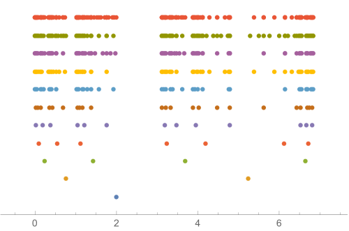
Figure 8. Roots of $\gamma_{n}$ for $n=1,\dotsc,11$ ($n$ increases on the vertical axis).

Proposition 3.15.

The degree of $\gamma_{n}$ is

$$\operatorname{deg}(\gamma_{n}) =\frac{2}{\sqrt{7}}\biggl{(}\rho_{1}^{n}\cos\bigl{(}\phi+\frac{2\pi}{3}\bigr{)}+\rho_{2}^{n}\cos\bigl{(}\phi+\frac{4\pi}{3}\bigr{)}+\rho_{3}^{n}\cos\phi\biggr{)}$$

where $\phi=\frac{1}{3}\arctan(-3\sqrt{3})$ and

$$\rho_{1}=\frac{1}{3}\Bigl{(}1-2\sqrt{7}\cos\phi\Bigr{)}, \rho_{2}=\frac{1}{3}\Bigl{(}1-2\sqrt{7}\cos\bigl{(}\phi+\frac{2\pi}{3}\bigr{)}\Bigr{)}, \rho_{3}=\frac{1}{3}\Bigl{(}1+2\sqrt{7}\cos\bigl{(}\phi+\frac{\pi}{3}\bigr{)}\Bigr{)}.$$

Moreover the degrees of $\gamma_{n}$ and $\eta_{n}$ are related by

(3.21) $$\operatorname{deg}(\eta_{n})=\operatorname{deg}(\gamma_{n})-2^{\lfloor\frac{n}{2}\rfloor}$$

where $\lfloor\frac{n}{2}\rfloor$ is the greatest integer less than $\frac{n}{2}$.

Proof.

Observe that $\eta_{1}=\gamma_{0}$ has degree $1$ and $\eta_{2}=\gamma_{1}$ has degree $2$, while $\gamma_{2}$ has degree $4$. This shows that (3.21) holds for $n=1,2$, and we suppose inductively that this holds for all $k\leq n-1$. Examining the recursion in Corollary (3.13) we see from the inductive hypotheses that each bracketed term on the right has the same degree as its included $\gamma$ term, and therefore that

(3.22) $$\operatorname{deg}(\gamma_{n}-2\eta_{n})=\operatorname{deg}(\gamma_{n-1})+2\operatorname{deg}(\gamma_{n-2})-\operatorname{deg}(\gamma_{n-3}).$$

However $\gamma_{n-3}\eta_{n}=\gamma_{n-1}\eta_{n-2}^{2}$ and thus there is a similar recursion

$$\operatorname{deg}(\eta_{n}) =\operatorname{deg}(\gamma_{n-1})+2\operatorname{deg}(\eta_{n-2})-\operatorname{deg}(\gamma_{n-3})$$

(3.23) $$=\operatorname{deg}(\gamma_{n-1})+2\operatorname{deg}(\gamma_{n-2})-2^{\lfloor(n-2)/2\rfloor+1}-\operatorname{deg}(\gamma_{n-3}),$$

where we have substituted the inductive hypothesis (3.21) to obtain the second expression. Comparing this to (3.22) proves that $\operatorname{deg}(\eta_{n})<\operatorname{deg}(\gamma_{n})$ and thereby reduces (3.22) to

(3.24) $$\operatorname{deg}(\gamma_{n})=\operatorname{deg}(\gamma_{n-1})+2\operatorname{deg}(\gamma_{n-2})-\operatorname{deg}(\gamma_{n-3}).$$

Comparing this to (3.23) proves that (3.21) holds for $k=n$ and therefore for all $n$ by induction.

The recursion in (3.24) can be solved by writing it as a matrix equation and computing an appropriate matrix power. The matrix involved has characteristic polynomial $\rho^{3}-\rho^{2}-2\rho+1$, the roots $\rho_{j}$, $j=1,2,3$ of which are as given in the statement of the lemma. The rest of the proof is standard. ∎

4. KNS Spectral Measure

For a sequence of graphs convergent in the metric 2.1 the Kesten–von-Neumann–Serre (KNS) spectral measure, defined in [28], is the weak limit of the (Neumann) spectral measures for the graphs in the sequence. In particular, for a blowup $G_{\infty}$ it is the limit of the normalized sum of Dirac masses $\delta_{\lambda_{j}}$ at eigenvalues of the Laplacian $L_{n}$ on $G_{n}$, repeated according to their multiplicity. Since the measure does not depend on which blowup $G_{\infty}$ we consider, we will henceforth just refer to the KNS spectral measure. Note that by Theorem 2.3 this is also the KNS spectral measure of the orbital Schreier graphs of the Basilica that do not have four ends.

Our first observation regarding the KNS spectral measure is that we can study it using the limit of the spectral measure for the Dirichlet Laplacian on $G_{n}$, or even the limit of the measure on Dirichlet-Neumann eigenfunctions on $G_{n}$.

Lemma 4.1.

The KNS spectral measure is the weak limit of the spectral measure for the Dirichlet Laplacian on $G_{n}$, which is given by

(4.1) $$\chi_{n}=\frac{1}{V_{n}-2}\sum_{\{\lambda_{j}:c_{n}(\lambda_{j})=0\}}\delta_{\lambda_{j}}\\ =\sum_{k=1}^{n}\sum_{\{\lambda_{j}:\gamma_{k}(\lambda_{j})=0\}}\frac{S_{n-k}}{V_{n}-2}\delta_{\lambda_{j}}.$$

Moreover, the support of the KNS spectral measure is contained in the closure of the union over $n$ of the set of Dirichlet-Neumann eigenvalues for the Laplacian on $G_{n}$.

Proof.

From Corollary 3.9 the number of eigenfunctions of $L_{n}$ that are Dirichlet but not Neumann is no larger than $\deg(\gamma_{n})+\frac{n}{2}$. Accordingly the number that are Neumann but not Dirichlet-Neumann does not exceed $2+\deg(\gamma_{n})+\frac{n}{2}$. But from Proposition 3.15 the degree of $\gamma_{n}$ is bounded by a multiple of $\rho^{n}$ for some $\rho<2$ (because we can check all $\rho_{j}<2$). The number of eigenvalues of $L_{n}$ grows like $2^{n}$ from Lemma 2.5, so the proportion of eigenvalues corresponding to eigenfunctions that are not Dirichlet-Neumann is bounded by a multiple of $(\rho/2)^{n}$ and makes no contribution to the mass in the limit. It follows that we get the same limit measure whether we take the limit of the spectrum of the Neumann Laplacian $L_{n}$, or the Dirichlet Laplacian on $G_{n}$, or even the normalized measure on the eigenvalue corresponding to Dirichlet-Neumann eigenfunctions.

The computation (4.1) can be justifed using the factorization in Theorem 3.11 and the observation that the degree of $c_{n}$ is two less than the number of vertices of $G_{n}$, which was computed in Lemma 2.5. A graph of the spectral measure $\chi_{11}$ for $G_{11}$ is in Figure 9.

For the final statement of the lemma, observe that if $\lambda$ is in the support of the KNS measure and $U$ is a neighborhood of $\lambda$ then $U$ has positive KNS measure and hence there is a lower bound on the $G_{n}$-spectral measure of $U$ for all sufficiently large $n$. We just saw that the proportion of the $G_{n}$ spectral measure that is not on Dirichlet-Neumann eigenvalues goes to zero as $n\to\infty$, so $U$ must contain a Dirichlet-Neumann eigenvalue. Thus the support of the KNS measure is in the closure of the union of the Dirichlet-Neumann spectra. ∎

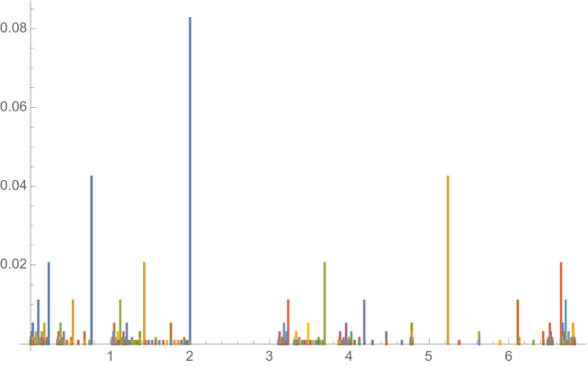
Figure 9. Spectral measure $\chi_{11}$ of the Dirichlet Laplacian on $G_{11}$.

We can compute the multiplicities and the degree of $c_{n}$, so it is easy to estimate the weights at the eigenvalues that occur as roots of $\gamma_{k}$.

Lemma 4.2.

$$\Bigl{|}\frac{S_{n-k}}{V_{n}-2}-\frac{1}{6}2^{-k}\Bigr{|}\leq\frac{n+5}{2^{n+1}}.$$

Proof.

Compute using the formulas for $V_{n}$ and $S_{n}$ from Lemma 2.5 and Theorem 3.11 that

$$\Bigl{|}\frac{S_{n-k}}{V_{n}-2}-\frac{1}{6}2^{-k}\Bigr{|} =\frac{1}{6}\Bigl{|}\frac{9+(23-6(n-k))(-1)^{n-k}+2^{n-k+2}}{2^{n+2}-3+(-1)^{n+1}}-2^{-k}\Bigr{|}$$

$$=\frac{1}{6}\Bigl{|}\frac{9(1-2^{-k})+(23-6(n-k)+2^{-k})(-1)^{n-k}}{2^{n+2}-3+(-1)^{n+1}}\Bigr{|}$$

$$\leq\frac{n-k+6}{2^{n+1}}\qed$$

This tells us that for fixed $k$ and large $n\gg k$ the measure $\chi_{n}$ has atoms of approximately weight $2^{-k}/6$ at each eigenvalue of the Dirichlet Laplacian on $G_{k}$.

Corollary 4.3.

The support of the KNS spectral measure is the closure of the union of the Dirichlet spectra of the $G_{n}$.

Proof.

In Lemma 4.1 we saw that the support of the KNS spectral measure is in the closure of the union of the Dirichlet-Neumann spectra, which is clearly contained in the closure of the union of the Dirichlet spectra.

Conversely, if $\lambda$ is a Dirichlet eigenvalue on $G_{n}$ then there is a smallest $k\leq n$ so $\lambda$ is an eigenvalue of $G_{k}$. Sending $n\to\infty$ we find from Lemma 4.2 that the KNS measure will have an atom of weight $\frac{1}{6}2^{-k}$ at $\lambda$, which is therefore in the support of the KNS measure. ∎

To get more precise statements comparing $\chi_{m}$ to the limiting KNS measure it is useful to fix $m$ and estimate the amount of mass in $\chi_{n}$ that lies on eigenvalues from $G_{k}$, $k>m$. Arguing as in the proof of Lemma 4.1 we might anticipate that this proportion is, in the limit as $n\to\infty$, bounded by $(\rho/2)^{m}$, so that the eigenvalues from $G_{m}$ capture all but a geometrically small proportion of the limiting KNS spectral measure. We want a more precise statement, for which purpose we establish the following lemma.

Lemma 4.4.

If $\rho=\rho_{j}$ is one of the values in Proposition 3.15 then

$$\sum_{k=m+1}^{n}S_{n-k}\rho^{k} =\frac{1}{36}\rho^{m+1}\Bigl{(}2^{n-m+2}\rho(\rho+1)+(5\rho^{2}-4\rho-18)(-1)^{n-m}$$

$$\quad+6\rho(2-\rho)(-1)^{n-m}(n-m)+9(2-\rho^{2})\Bigr{)}$$

Proof.

Compute, using $S_{0}=1$, $S_{1}=0$ and the recursion (3.16) for $S_{n}$, $n\geq 2$, that

$$\sum_{k=m+1}^{n+1}S_{n+1-k}\rho^{k} =\rho^{n+1}+\sum_{k=m+1}^{n-1}S_{n+1-k}\rho^{k}$$

$$=\rho^{n+1}+\sum_{k=m+1}^{n-1}\Bigl{(}S_{n-k}+2S_{n-1-k}-\frac{1}{2}\bigl{(}1-(-1)^{n-k}\bigr{)}\Bigr{)}\rho^{k}$$

$$=\rho^{n+1}-\rho^{n}+\sum_{m+1}^{n}S_{n-k}\rho^{k}+\sum_{m+1}^{n-1}2S_{n-1-k}\rho^{k}$$

$$\quad-\frac{\rho^{n}-\rho^{m+1}}{2(\rho-1)}+(-1)^{n}\frac{(-\rho)^{n}-(-\rho)^{m+1}}{2(-\rho-1)}$$

$$=\sum_{m+1}^{n}S_{n-k}\rho^{k}+\sum_{m+1}^{n-1}2S_{n-1-k}\rho^{k}$$

$$\quad+\rho^{n}\Bigl{(}\rho-1-\frac{\rho}{\rho^{2}-1}\Bigr{)}+\frac{\rho^{m+1}}{2}\Bigl{(}\frac{1}{\rho-1}-\frac{(-1)^{n-m}}{\rho+1}\Bigr{)}$$

and conveniently the coefficient of $\rho^{n}$ has a factor $(\rho^{3}-\rho^{2}-2\rho+1)$, and the values $\rho_{j}$ are precisely the roots of this equation (see the end of the proof of Proposition 3.15). Thus we have a recursion for our desired quantity, with the form

$$\sum_{k=m+1}^{n+1}S_{n+1-k}\rho^{k}=\sum_{m+1}^{n}S_{n-k}\rho^{k}+\sum_{m+1}^{n-1}2S_{n-1-k}\rho^{k}+\frac{\rho^{m+1}}{2}\Bigl{(}\frac{1}{\rho-1}-\frac{(-1)^{n-m}}{\rho+1}\Bigr{)}.$$

The homogeneous part of the solution is $\bigl{(}c_{1}2^{n-m}+c_{2}(-1)^{n-m}\bigr{)}\rho^{m+1}$. The inhomogeneous part has terms $c_{3}\rho^{m+1}$ and $c_{4}(n-m)(-1)^{n-m}\rho^{m+1}$. It is easy to calculate that

$$c_{3}=\frac{-1}{4(\rho-1)}=\frac{(2-\rho^{2})}{4}$$

$$c_{4}=\frac{1}{6(\rho+1)}=\frac{\rho(2-\rho)}{6}$$

where the latter expression in each formula is from $\rho^{3}-\rho^{2}-2\rho+1=0$. Then one can compute $c_{1}$ and $c_{2}$ from the initial values $\sum_{m+1}^{m+1}S_{n-k}\rho^{k}=\rho^{m+1}$ and $\sum_{m+1}^{m+2}S_{n-k}\rho^{k}=\rho^{m+2}$, which themselves come from $S_{0}=1$, $S_{1}=0$, or directly verify that the expression in the lemma has these initial values. ∎

Corollary 4.5.

In the limit $n\to\infty$ the proportion of the spectral mass of $G_{n}$ that lies on eigenvalues of $G_{m}$ is

$$\frac{1}{3\sqrt{7}}\sum_{j}\cos\bigl{(}\phi+\frac{2j\pi}{3}\bigr{)}\rho_{j}^{2}(\rho_{j}+1)\bigl{(}\frac{\rho_{j}}{2}\bigr{)}^{m}$$

where $\phi=\frac{1}{3}\arctan(-3\sqrt{3})$ as in Proposition 3.15.

Proof.

Dividing $\sum_{k=m+1}^{n}S_{n-k}\rho_{j}^{k}$ by $V_{n}-2=\frac{1}{6}\bigl{(}2^{n+2}+(-1)^{n+1}-3\bigr{)}$, using the result of Lemma 4.4 and sending $n\to\infty$ gives

$$\lim_{n\to\infty}\frac{1}{V_{n}-2}\sum_{k=m+1}^{n}S_{n-k}\rho_{j}^{k}=\frac{1}{6}\rho_{j}^{2}(\rho_{j}+1)\bigl{(}\frac{\rho_{j}}{2}\bigr{)}^{m}$$

whereupon the result follows by substitution into the expression

$$\sum_{k=m+1}^{n}S_{n-k}\operatorname{deg}(\gamma_{k})=\frac{2}{\sqrt{7}}\sum_{j=1}^{3}\cos\bigl{(}\phi+\frac{2j\pi}{3}\bigr{)}\sum_{k=m+1}^{n}S_{n-k}\rho_{j}^{k}$$

from Proposition 3.15. ∎

A slightly more involved computation gives a bound on the $m$ needed to obtain a given proportion of the KNS spectral measure.

Theorem 4.6.

For any $\epsilon>0$ there is $m$ comparable to $|\log\epsilon|$ such that, for $n\geq m$, all but $\epsilon$ of the spectral mass of any $G_{n}$ is supported on eigenvalues of the Laplacian on $G_{m}$.

Proof.

Decompose the sum (4.1) into the sum $\sum_{k=1}^{m}$ over eigenvalues of the Laplacian on $G_{m}$ and $\sum_{m+1}^{n}$ of eigenvalues of the Laplacian on $G_{n}$ that are not in the $G_{m}$ spectrum. As in the previous proof, use Proposition 3.15 to write

$$\sum_{k=m+1}^{n}S_{n-k}\operatorname{deg}(\gamma_{k})=\frac{2}{\sqrt{7}}\sum_{j=1}^{3}\cos\bigl{(}\phi+\frac{2j\pi}{3}\bigr{)}\sum_{k=m+1}^{n}S_{n-k}\rho_{j}^{k}$$

and then estimate using Lemma 4.4. From the specific values of $\rho_{j}$ in Proposition 3.15 one determines

$$\sum_{k=m+1}^{n}S_{n-k}\rho_{1}^{k} \leq\frac{1}{36}|\rho_{1}|^{m+1}\Bigl{(}\frac{1}{3}2^{n-m+2}+25(n-m)+10\Bigr{)},$$

(4.2) $$\sum_{k=m+1}^{n}S_{n-k}\rho_{2}^{k} \leq\frac{1}{36}|\rho_{2}|^{m+1}\Bigl{(}\frac{2}{3}2^{n-m+2}+5(n-m)+36\Bigr{)},$$

$$\sum_{k=m+1}^{n}S_{n-k}\rho_{2}^{k} \leq\frac{1}{36}|\rho_{3}|^{m+1}\Bigl{(}\frac{11}{2}2^{n-m+2}+3(n-m)+21\Bigr{)}.$$

The largest of the $|\rho_{j}|$ is $|\rho_{3}|$, so we bound the terms not containing $2^{n-m+2}$ by $(n-m+2)|\rho_{3}|^{m+1}$. For the terms that do contain $2^{n-m+1}$ we use the readily computed fact that $|\rho_{1}|^{m+1}/3+2|\rho_{2}|^{m+1}/3\leq|\rho_{3}|^{m+1}/2$ for all $m$ and combine these to obtain

$$\sum_{k=m+1}^{n}S_{n-k}\operatorname{deg}(\gamma_{k})\leq\frac{2}{\sqrt{7}}\rho_{3}^{m+1}\Bigl{(}\frac{1}{6}2^{n-m+2}+(n-m+2)\Bigr{)}.$$

The contribution to the KNS spectral measure is computed by dividing by $V_{n}-2=\frac{1}{6}\bigl{(}2^{n+2}+(-1)^{n+1}-3\bigr{)}$, which was computed in Lemma 2.5. This is larger than $\frac{1}{6}2^{n+1}$ because $n\geq 1$, so from the above reasoning

$$\sum_{k=m+1}^{n}\frac{S_{n-k}}{V_{n}-2}\operatorname{deg}(\gamma_{k})\leq\frac{8}{\sqrt{7}}\Bigl{(}1+6(n-m+2)2^{-(n-m+2)}\Bigr{)}\Bigl{(}\frac{|\rho_{3}|}{2}\Bigr{)}^{m+1}$$

but $l2^{-l}$ is decreasing with maximum value $\frac{1}{2}$, so we readily obtain

$$\sum_{k=m+1}^{n}\frac{S_{n-k}}{V_{n}-2}\operatorname{deg}(\gamma_{k})\leq\frac{12}{\sqrt{7}}\Bigl{(}\frac{|\rho_{3}|}{2}\Bigr{)}^{m+1}<\epsilon$$

provided $m\geq C|\log\epsilon|$, where $C$ is a constant involving $\log\rho_{3}$. This estimate says that at most $\epsilon$ of the spectral mass can occur outside the spectrum of $G_{m}$ once $m$ is of size $C|\log\epsilon|$. ∎

5. Cantor structure of the spectrum

Our recursions for $c_{n}$ and $\gamma_{n}$ provide a method for computing the spectra of the $G_{n}$ for small $n$. Using a desktop computer we were able to compute them for $n\leq 14$. By direct computation from (4.2), using $(n-m)2^{1-(n-m)}\leq 1$, these eigenvalues constitute at least 39% of the spectrum (counting multiplicity) of any $G_{n}$, and the asymptotic estimate from Corollary 4.5 says that as $n\to\infty$ they capture approximately 76% of the KNS spectral measure. The result is shown in Figure 10.

Figure 10. The spectrum of $G_{14}$, illustrating gaps

Comparing Figures 8, 9 and 10 it appears that there are structural properties of the spectrum that are independent of $n$. These should be features of the dynamics described in Section 3. The main result of this section is that the support of the KNS spectral measure is a Cantor set. To prove this we use the dynamics established in Corollary 3.14, namely that for $n\geq 4$ the eigenvalues first seen at level $n$, which are the roots of $\gamma_{n}=\gamma_{n}(\lambda)$, are also precisely the roots of $\zeta_{n}=\gamma_{n}/\eta_{n}$, which satisfies the recursion

(5.1) $$\zeta_{n}-2=\Bigl{(}1+\frac{2}{\zeta_{n-1}}\Bigr{)}(\zeta_{n-2}^{2}-4)$$

The initial data were given in (3.20).

We begin by describing an escape criterion under which future iterates of (5.1) do not get close to zero, and therefore cannot produce values in the spectrum.

Lemma 5.1.

If $n\geq 4$ and $|\zeta_{n-2}|>2$ and $|\zeta_{n-1}|>2$ then $|\zeta_{m}|\to\infty$ as $m\to\infty$.

Proof.

Since $|\zeta_{n-1}|>2$ we have $1+\frac{2}{\zeta_{n-1}}>0$. At the same time, $\zeta_{n-2}^{2}>4$, so $\zeta_{n}>2$ from (5.1). The same argument gives $\zeta_{n+1}>2$. Now $\zeta_{n+1}>2$ implies $1+\frac{2}{\zeta_{n+1}}>1$ and thus from (5.1)

$$\zeta_{n+2}-2>\zeta_{n}^{2}-4=(\zeta_{n}-2)(\zeta_{n}+2)>4(\zeta_{n}-2).$$

This argument applies for all $\zeta_{m}$, $m\geq n+2$, so

$$\zeta_{m}\geq 2^{m-n-2}\bigl{(}\min\{\zeta_{n},\zeta_{n+1}\}-2\bigr{)}\to\infty$$

as $m\to\infty$. ∎

A similar analysis gives the following

Lemma 5.2.

Suppose $n\geq 3$. For any $\delta\in(0,2)$ there is $k$ such that the region $|\zeta_{n-1}|>2$, $\zeta_{n}\in(2-\delta,2)$ contains a root of $\zeta_{n+2k}$.

Proof.

Observe that if $|\zeta_{n+2j-1}>2|$ and $\zeta_{n+2j}\in(0,2)$ then from (5.1)

(5.2) $$\zeta_{n+2j+1}-2=\Bigl{(}1+\frac{2}{\zeta_{n+2j}}\Bigr{)}(\zeta_{n+2j-1}-2)(\zeta_{n+2j-1}+2)$$

is a product of positive terms, so $\zeta_{n+2j+1}>2$.

Now suppose $\zeta_{n+2j+1}>2$. Then the map $\zeta_{n+2j}\mapsto\zeta_{n+2j+2}$ is continuous and has $2\mapsto 2$, so it takes an interval $(2-\delta_{j},2)\subset(0,2)$ to an interval covering $(2-2\delta_{j},2)$ because subsitution into (5.1) gives

$$2-\delta_{j}\mapsto 2-\delta_{j}(4-\delta_{j})\Bigl{(}1+\frac{2}{\zeta_{n+2j+1}}\Bigr{)}<2-2\delta_{j}.$$

It follows from the above reasoning that if we begin with the region $|\zeta_{n-1}|>2$ and $\zeta_{n}\in(2-\delta,2)$ then the inductive statement that the $j^{\text{th}}$ iterated image satisfies $\zeta_{n+2j-1}>2$ and $\zeta_{n+2j}\in(0,2)$ for $1\leq j\leq k$ must fail before $k>\log_{2}\delta$. Moreover it will fail because the image $\zeta_{n+2k}$ is an interval that strictly covers $(0,2)$, so there is a zero of $\zeta_{n+2k}$ in the required region. ∎

We now wish to proceed by analyzing a few steps of the orbit of a point $\tilde{\lambda}$ at which $\zeta_{n}(\tilde{\lambda})=0$. This is complicated a little by the fact (immediate from (5.1)) that $\zeta_{n+1}$ may have a pole at $\tilde{\lambda}$. We need a small lemma.

Lemma 5.3.

If $\zeta_{n}(\tilde{\lambda})=0$ then $\zeta_{m}(\tilde{\lambda})\not\in\{-2,2\}$ for $m<n$.

Proof.

Under the hypothesis there are no other $\gamma_{m}$ which vanish at $\tilde{\lambda}$, so $\zeta_{m}$, $m<n$ has neither zeros nor poles at $\tilde{\lambda}$; we use this fact several times without further remark.

There are some initial cases for which (5.1) does not assist in computing $\zeta_{m}(\tilde{\lambda})$. Evidently the statement of the lemma is vacuous if $n=1$. If $n=2$ we compute $\tilde{\lambda}=3\pm\sqrt{5}$, so $\zeta_{1}(\tilde{\lambda})=\tilde{\lambda}-2\not\in\{-2,2\}$. If $n=3$ it is more useful to check that both $\zeta_{1}(\tilde{\lambda})=\pm 2$ and $\zeta_{2}(\tilde{\lambda})=-2$ correspond to $\tilde{\lambda}\in\{0,4\}$, while $\zeta_{2}(\tilde{\lambda})=-2$ implies $\tilde{\lambda}=4\pm 2\sqrt{2}$, because these are exactly the four solutions of $\zeta_{3}(\tilde{\lambda})=2$. This verifies the lemma if $n=1,2,3$. Moreover in the case $n\geq 4$ the equivalence of $\zeta_{2}(\tilde{\lambda})\in\{-2,2\}$ with $\zeta_{3}(\tilde{\lambda})=2$ may also be used to exclude both of these possibilities, because if they hold then iteration of (5.1) gives $\zeta_{m}(\tilde{\lambda})=2$ for all $m\geq 3$ in contradiction to $\zeta_{n}(\tilde{\lambda})=0$.

Now with $n\geq 4$ we use (5.1) to see that if there were $3\leq m<n$ for which $\zeta_{m}(\tilde{\lambda})=-2$ then both $\zeta_{m+1}(\tilde{\lambda})=2$ and $\zeta_{m+1}(\tilde{\lambda})=2$, so that $\zeta_{m+k}(\tilde{\lambda})=2$ for all $k\geq 1$ in contradiction to $\zeta_{n}(\tilde{\lambda})=0$. Combining this with our initial cases, $\zeta_{m}(\tilde{\lambda})\neq-2$ for all $m<n$.

Finally, if there were an $m$ with $4\leq m<n$ and $\zeta_{m}(\tilde{\lambda})=2$ then taking the smallest such $m$ and applying (5.1) would give $\zeta_{m-2}(\tilde{\lambda})=2$ because the other two roots are $\zeta_{m-1}(\tilde{\lambda})=-2$ and $\zeta_{m-2}(\tilde{\lambda})=-2$, both of which have been excluded. Since $m\geq 4$ was minimal we have $m=4$ or $m=5$, but then either $\zeta_{2}(\tilde{\lambda})=2$ or $\zeta_{3}(\tilde{\lambda})=2$, both of which we excluded in our initial cases. ∎

Theorem 5.4.

If $\zeta_{n}(\tilde{\lambda})=0$ then there is $\delta>0$ so that either the interval $I_{-}=(\tilde{\lambda}-\delta,\tilde{\lambda})$ or the interval $I_{+}=(\tilde{\lambda},\tilde{\lambda}+\delta)$ is a gap, meaning it does not intersect the Dirichlet Laplacian spectrum of $G_{m}$ for any $m\in\mathbb{N}$. By contrast, there is a sequence $k_{j}\to\infty$ such that the other interval contains a sequence of Dirichlet eigenvalues for the Laplacian on $G_{n+2k_{j}}$ that accumulate at $\tilde{\lambda}$.

Proof.

Recall from Proposition 3.7 that the zeros of $\gamma_{n}$ and thus of $\zeta_{n}$ are simple. The definition of $\zeta_{n}=\gamma_{n}/\zeta_{n}$ ensures its zeros are also distinct from the zeros and poles of $\zeta_{m}$ $m<n$, so we may initially take $\delta$ so that $\zeta_{n}$ is positive on one of $I_{-}$, $I_{+}$ and negative on the other, and such that each $\zeta_{m}$, $m<n$ has constant sign on $I=(\tilde{\lambda}-\delta,\tilde{\lambda}+\delta)$.

Lemma 5.3 ensures $\zeta_{n-2}(\tilde{\lambda})^{2}-4\neq 0$, so (5.1) and simplicity of the root of $\zeta_{n}$ at $\tilde{\lambda}$ ensure $\zeta_{n+1}$ has a simple pole at $\tilde{\lambda}$ if $n\geq 3$. For $n=1,2$ the same fact can be verified directly from the inital data (3.20) for the dynamics. In particular, $|\zeta_{n+1}(\lambda)|\to\infty$ as $\lambda\to\tilde{\lambda}$. By reducing $\delta$, if necessary, we may assume $|\zeta_{n+1}(\lambda)|>2$ on $I\setminus\{\tilde{\lambda}\}$.

We use the preceding to linearly approximate $\zeta_{n+j}$ for $j=2,3$. Since (5.1) is a dynamical system on rational functions we can linearize around a pole, but in order to use this dynamics we need $n\geq 3$. Temporarily write $t=\lambda-\tilde{\lambda}$ and use $\simeq$ for equality up to $O(t^{2})$ so simplicity of the root of $\zeta_{n}$ at $\tilde{\lambda}$ implies there is a non-zero $\alpha$ with $\zeta_{n}(\lambda)\simeq\alpha t$ and the fact that $\zeta_{n-1}^{2}\neq 4$ gives $\beta,\beta^{\prime}$ with $\beta\neq 0$ so $(\zeta_{n-1}^{2}-4)\simeq\beta+\beta^{\prime}t$. Then we compute from (5.1):

$$\frac{2}{\zeta_{n+1}} =\frac{2\zeta_{n}}{2\zeta_{n}+(\zeta_{n}+2)(\zeta_{n-1}^{2}-4)}$$

(5.3) $$\simeq\frac{2\alpha t}{2\alpha t+(\alpha t+2)(\beta+\beta^{\prime}t)}\simeq\frac{\alpha}{\beta}t,$$

and therefore

$$\zeta_{n+2} =2+\Bigl{(}1+\frac{2}{\zeta_{n+1}}\Bigr{)}(\zeta_{n}^{2}-4)$$

(5.4) $$\simeq 2+\Bigl{(}1+\frac{\alpha}{\beta}t\Bigr{)}(\alpha^{2}t^{2}-4)\simeq-2-\frac{4\alpha}{\beta}t.$$

The preceding is valid for $n\geq 3$, but if $n=2$ then $\tilde{\lambda}\in\{3-\sqrt{5},3+\sqrt{5}\}$ and a linearization of $2\zeta_{3}^{-1}$ like (5.3) is readily computed from (3.20) while the argument of (5.4) is valid for $\zeta_{4}$. Moreover, if $n=1$ then $\tilde{\lambda}=2$ and linearizations for both $2\zeta_{2}^{-1}$ and $\zeta_{3}$ can again be computed directly from (3.20). Thus (5.3) and (5.4) are valid for all $n\geq 1$.

Since $\alpha$ and $\beta$ are non-zero, the linearizations show that $\zeta_{n+2}(\lambda)<-2$ for $t$ in an interval on the side of $0$ where $\frac{\alpha}{\beta}t>0$, meaning that $\lambda$ is on the corresponding side of $\tilde{\lambda}$. By reducing $\delta$, if necessary, we conclude $\zeta_{n+2}<-2$ on one of $I_{+}$ or $I_{-}$. At this point we have both $|\zeta_{n+1}(\lambda)|>2$ and $|\zeta_{n+2}(\lambda)|>2$ on exactly one of the two intervals $I_{-}$ or $I_{+}$, and since $n+1\geq 2$ we can apply Lemma 5.1 to find that this interval does not contain zeros of $\zeta_{m}$ for any $m>n$. Since it was also selected so as to not contain zeros of $\zeta_{m}$ for $m\leq n$ we have proved that one of these intervals is a gap.

Turning to the other interval, where $\frac{\alpha}{\beta}t<0$, we will need two more iterations of the linearized dynamics. The index $n$ is now large enough that we need only apply (5.1) to (5.3) and (5.4), which gives:

$$\zeta_{n+3} =2+\frac{(\zeta_{n+2}+2)}{\zeta_{n+2}}(\zeta_{n+1}^{2}-4)$$

$$\simeq 2+\frac{-\frac{4\alpha}{\beta}t}{(-2-\frac{4\alpha}{\beta}t)}\Bigl{(}\frac{4}{(\frac{\alpha}{\beta}t)^{2}}-4\Bigr{)}$$

(5.5) $$\simeq 2+\frac{8}{(1+\frac{2\alpha}{\beta}t)(\frac{\alpha}{\beta}t)},$$

so that $2\zeta_{n+3}^{-1}\simeq\frac{3\alpha}{16\beta}t$. A second application gives

$$\zeta_{n+4} =2+\Bigl{(}1+\frac{2}{\zeta_{n+3}}\Bigr{)}(\zeta_{n+2}^{2}-4)$$

$$\simeq 2+\Bigl{(}1+\frac{3\alpha}{16\beta}t\Bigr{)}\Bigl{(}\bigl{(}-2-\frac{4\alpha}{\beta}t\bigr{)}^{2}-4\Bigr{)}$$

(5.6) $$\simeq 2+\frac{16\alpha}{\beta}t.$$

Now suppose we are given $0<\delta^{\prime}<\delta$. By reducing $\delta^{\prime}$ if necessary we find from (5.6) that the map $\zeta_{n}\mapsto\zeta_{n+4}$ takes the side of the interval $|\lambda-\tilde{\lambda}|=|t|<\delta^{\prime}$ that lies in the non-gap interval, meaning $\frac{\alpha}{\beta}t<0$, to an interval of the form $(2-\delta^{\prime\prime},2)\subset(0,2)$. At the same time, and again reducing $\delta^{\prime}$ if necessary, we can assume from (5.5) that $|\zeta_{n+3}|>2$ on this interval. But then Lemma 5.2 is applicable to $\zeta_{n+3}$ and $\zeta_{n+4}$ and we find there is $k$ so that $\zeta_{n+4+2k}$ has a root in the interval. Since this argument was applicable to any $0<\delta^{\prime}<\delta$ we conclude that the roots of the rational functions $\zeta_{n+2k}$ accumulate to $\tilde{\lambda}$ as $k\to\infty$ within the non-gap interval. ∎

Corollary 5.5.

The support of the KNS spectrum is a Cantor set. In particular it is uncountable and has countably many gaps.

Proof.

Recall from Corollary 4.3 that the support of the KNS spectral measure is the closure of the union of the set of Dirichlet Laplacian eigenvalues on $G_{n}$. For $\tilde{\lambda}$ a Dirichlet eigenvalue there is a least $n$ for which it is such, and the definition of $\zeta_{n}$ ensures $\zeta_{n}(\tilde{\lambda})=0$. But then Theorem 5.4 provides a sequence $k_{j}$ and roots of $\zeta_{n+2k_{j}}$ that accumulate at $\tilde{\lambda}$. This shows each Dirichlet eigenvalue for $G_{n}$ is a limit point of such eigenvalues, and therefore the support of the KNS spectrum is perfect.

If there was an interval in the support of the KNS spectrum then by Corollary 4.3 it would contain an interior point $\tilde{\lambda}$ from the Dirichlet spectrum on some $G_{n}$. By assuming $n$ is the first index for which the eigenvalue $\tilde{\lambda}$ occurs we have $\zeta_{n}(\tilde{\lambda})=0$, so Theorem 5.4 provides a gap on one side of $\tilde{\lambda}$ and we have a contradiction. Accordingly the connected components of the support of the KNS spectrum are points and the set is totally disconnected.

We have shown that the support of the KNS spectrum is perfect and totally disconnected, so it is a Cantor set. ∎

The construction in the proof of Theorem 5.4 allows us to find specific gaps by taking preimages of regions that the theorem ensures will escape under the dynamics (5.1) and will therefore not contain eigenvalues. One can visualize these dynamics using graphs in $\mathbb{R}^{2}$, with coordinates $x=\zeta_{2}$ and $y=\zeta_{3}$. We are interested only in those values that are given by (3.20), which are shown as thick curves on the graphs in Figure 11. The graph also shows the preimages of the escape region from Theorem 5.4 for small $n$. More precisely, these sets are where both $|\zeta_{n-2}|>2$ and $|\zeta_{n-1}|>2$. Note that the intersections of the shaded regions with the thick curves correspond to intervals of $\lambda\in\mathbb{R}$ which cannot contain spectral values for any larger $n$, and are therefore gaps in the spectrum of $\Delta_{n}$ for all $n$. Using (5.1) it is fairly easy to determine the endpoints of the intervals for any specified $n$. If it were possible to give good estimates for the sizes of these intervals one could resolve the following question.

Problem 5.6.

Determine whether the closure of the union of the spectra of the $L_{n}$ has zero Lebesgue measure or give estimates for its Hausdorff dimension.

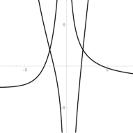
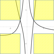
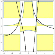
Figure 11. Graphs of $(\zeta_{1}(\lambda),\zeta_{2}(\lambda))$ (left) superimposed on escape regions $|\zeta_{2}|>2,|\zeta_{3}|>2$ (middle) and $|\zeta_{4}|>2,|\zeta_{5}|>2$ (right).

6. A generic set of blowups of the graphs $G_{n}$ with Pure Point Spectrum

Recall from Definition 2.2 that a blow-up $G_{\infty}$ is the direct limit of a system $(G_{k_{n}},\iota_{k_{n}})$ with cannonical graph morphisms $\tilde{\iota}_{k_{n}}:G_{k_{n}}\to G_{\infty}$ and the Laplacian $L_{\infty}$ on $G_{\infty}$ (from Definition 2.4) at $\tilde{\iota}_{k_{n}}(x)$ for a non-boundary point $x\in G_{k_{n}}$ coincides with $L_{k_{n}}$ on $\tilde{\iota}_{k_{n}}(G_{k_{n}})$, as in (2.3). We will write $\tilde{G}_{k_{n}}=\tilde{\iota}_{k_{n}}(G_{k_{n}})$ for the cannonical copy of $G_{k_{n}}$ in $G_{\infty}$.

For the following lemma, note that $\tilde{\iota}_{k_{n}}$ can fail to be injective at the boundary points of $G_{k_{n}}$, but $f\circ\tilde{\iota}_{k_{n}}^{-1}$ is well-defined for a Dirichlet eigenfunction $f$ because $f=0$ at the boundary points.

Lemma 6.1.

If $f$ is a Dirichlet-Neumann eigenfunction of $L_{k_{n}}$ on $G_{k_{n}}$ then setting $F=f\circ\tilde{\iota}_{k_{n}}^{-1}$ on $\tilde{G}_{k_{n}}$ and zero elsewhere defines an eigenfunction of $L_{\infty}$ with the same eigenvalue and infinite multiplicity.

Proof.

Let $\lambda$ be the eigenvalue of $L_{k_{n}}$ corresponding to $f$. Using (2.3) we have immediately that

(6.1) $$L_{\infty}F(\tilde{\iota}_{k_{n}}(x))=L_{k_{n}}f(x)=\lambda f(x)=\lambda F(\tilde{\iota}_{k_{n}}(x))$$

if $x$ is not a boundary point of $G_{k_{n}}$. If $x$ is a boundary point of $G_{k_{n}}$ then $\tilde{\iota}_{k_{n}}(x)$ may have neighbors in $G_{\infty}$ that are outside $\tilde{G}_{k_{n}}$, but since $F$ vanishes at these points we still have $L_{\infty}F(\tilde{\iota}_{k_{n}}(x))=L_{k_{n}}f(x)$ and therefore (6.1) is still valid. It remains to see $L_{\infty}F(y)=\lambda F(y)$ for $y\not\in\tilde{G}_{k_{n}}$, but for such $y$ we have $L_{\infty}F(y)=0=\lambda F(y)$ because $F$ vanishes at $y$ and its neighbors; some of these neighbors may be in $\tilde{G}_{k_{n}}$, in which case the fact that $F$ vanishes uses the Dirichlet property of $f$. The corresponding eigenvalue has infinite multiplicity simply because there are an infinite number of distinct copies of any $G_{m}$ in $G_{\infty}$ ∎

The eigenvalues coming from Dirichlet-Neumann eigenfunctions not only have infinite multiplicity. According to Theorem 4.6 they support an arbitrarily large proportion of the KNS spectral mass of $L_{\infty}$. Even more is true for a certain class of blowups, for which we can show that spectrum is pure-point, with the set of Dirichlet-Neumann eigenfunctions generated at finite scales having dense span in $l^{2}$. Our proof closely follows an idea used to prove similar results for blow-ups of two-point self-similar graphs and Sierpinski Gaskets [38, 55].

Definition 6.2.

The subspace $l^{2}_{a}\subset l^{2}$ consists of the finitely supported functions that are antisymmetric in the following sense. The function $f\in l^{2}_{a}$ if there is $n$ such that $k_{n}-k_{n-1}=1$, $f$ is supported on $\tilde{\iota}_{k_{n-1}}$, and $g=f\circ\tilde{\iota}_{k_{n}}$ on $G_{k_{n}}$ satisfies $g=-g\circ\Phi_{k_{n}}$. See Figure 12.

Figure 12. A function from $l^{2}_{a}$ is supported and antisymmetric on a copy of $G_{k_{n-1}}$ in $G_{k_{n}}$ with $k_{n}-k_{n-1}=1$.

Lemma 6.3.

The space $l^{2}_{a}$ is invariant under $L_{\infty}$. Any eigenfunction of the restriction of $L_{\infty}$ to $l^{2}_{a}$ is also an eigenfunction of $L_{\infty}$ and the corresponding eigenvalue has infinite multiplicity. Moreover $l^{2}_{a}$ is contained in the span of the finitely supported eigenfunctions of $L_{\infty}$.

Proof.

The invariance is evident from the fact that $L_{k_{n}}$ is symmetric under $\Phi_{k_{n}}$ for each $n$ and (2.3). Suppose $f$ is an eigenfunction of the restriction of $L_{\infty}$ to $l^{2}_{a}$. Then there is $n$ as in Defintion 6.2, meaning $g=f\circ\tilde{\iota}_{k_{n}}$ satisfies $g=-g\circ\Phi_{k_{n}}$ and $g$ is supported on the copy of $G_{k_{n}-1}$ in $G_{k_{n}}$. It follows from parts (2) and (3) of Proposition 3.4 that $g$ is a Dirichlet-Neumann eigenfunction on $G_{k_{n}}$, and applying Lemma 6.1 shows $f$ is an eigenfunction of $L_{\infty}$ and the eigenvalue has infinite multiplicity.

Now any function in $l^{2}_{a}$ has the structure described in Definition 6.2 and is therefore in the span of the Dirichlet-Neumann eigenfunctions of $L_{k_{n}}$ for the $n$ given in that definition, and as was just mentioned, Lemma 6.1 provides that these extend to $G_{\infty}$ by zero to give finitely supported eigenfunctions of $L_{\infty}$. ∎

Theorem 6.4.

If the blowup $(G_{k_{n}},\iota_{k_{n}})$ is such that both $k_{n+1}-k_{n}=1$ and $k_{n+1}-k_{n}=2$ occur for infinitely many $n$ then the antisymmetric subspace $l^{2}_{a}$ is dense in $l^{2}$ and hence the spectrum of $L_{\infty}$ is pure point and there is an eigenbasis of finitely-supported antisymmetric eigenfunctions.

Proof.

Suppose $f\perp l^{2}_{a}$. It will be useful to have some notation for the various subsets, subspaces and functions we encounter. For fixed $n<m<\infty$ let us write $\iota^{\prime}_{k_{n},k_{m}}=\iota_{k_{m-1}}\circ\dotsm\circ\iota_{k_{n}}:G_{k_{n}}\to G_{k_{m}}$ and $G_{k_{n}}^{\prime}=\iota^{\prime}_{k_{n},k_{m}}(G_{k_{n}}\setminus\partial G_{k_{n}})$ for the image of $G_{k_{n}}$, less its boundary points, in $G_{k_{m}}$ and $G_{k_{n}}^{\prime\prime}=\tilde{\iota}_{k_{n}}(G_{k_{n}}\setminus\partial G_{k_{n}})$ for the corresponding image in $G_{\infty}$. We will write $P_{k_{n}}^{\prime\prime}f$ for the restriction of $f$ to $G_{k_{n}}^{\prime\prime}$, and $P_{n}^{\prime}f=P_{n}f\circ\tilde{\iota}_{k_{m}}$ for the corresponding function on $G_{k_{m}}$. We frequently use the fact that, under counting measure, the integral of a function supported on $\tilde{G}_{k_{n}}$ may also be computed on $G_{k_{n}}$ or $G_{k_{m}}$.

The argument proceeds as follows. Since $f\in l^{2}$ we can take $n$ so large that $\|P_{n}^{\prime\prime}f\|_{2}\geq\frac{2}{3}\|f\|_{2}$. Using the hypothesis, we choose $m>n$ to be the smallest number with the property that $k_{m-1}-k_{m-2}=1$ and $k_{m}-k_{m-1}=2$. Now we antisymmetrize $P_{n}^{\prime\prime}f$ with respect to $\Phi_{k_{m}}$ and take its inner product with $f$; this makes sense because $P_{n}^{\prime\prime}f$ corresponds to a function on $G_{k_{n}}$ and hence $G_{k_{m}}$. It will be convenient to do it on $G_{k_{m}}$.

Let $g(x)=P_{n}^{\prime}f-P_{n}^{\prime}f\circ\Phi_{k_{m}}$. Notice that $g=0$ at the points where $\tilde{\iota}_{k_{m}}$ is non-injective, so $F=g\circ\tilde{\iota}_{k_{m}}^{-1}$ is well-defined on $\tilde{G}_{k_{m}}\subset G_{\infty}$ and extending by zero to the rest of $G_{\infty}$ we have $F\in l^{2}_{a}$. From this and $f\perp l^{2}_{a}$,

$$0 =\langle f,F\rangle_{l^{2}}=\bigl{\langle}f\circ\tilde{\iota}_{k_{m}},g\bigr{\rangle}_{l^{2}_{k_{m}}}$$

$$=\langle f\circ\tilde{\iota}_{k_{m}},P_{n}^{\prime}f\rangle_{l^{2}_{k_{m}}}-\langle f\circ\tilde{\iota}_{k_{m}},P_{n}^{\prime}f\circ\Phi_{k_{m}}\rangle_{l^{2}_{k_{m}}}$$

$$=\langle f,P_{n}f\rangle_{l^{2}}-\langle f\circ\tilde{\iota}_{k_{m}}\circ\Phi_{k_{m}},P_{n}^{\prime}f\rangle_{l^{2}_{k_{m}}}$$

$$=\|P_{n}^{\prime\prime}f\|_{l^{2}}^{2}-\langle f|_{\tilde{\iota}_{k_{m}}\circ\Phi_{k_{m}}(G_{k_{n}}^{\prime})},P_{n}f\rangle_{l^{2}}$$

However our choice of $m$ ensures that $\Phi_{k_{m}}(G_{k_{n}}^{\prime})$ does not intersect $G_{k_{n}}^{\prime}$ and thus $\tilde{\iota}_{k_{m}}\circ\Phi_{k_{m}}(G_{k_{n}}^{\prime})$ does not intersect $G_{k_{n}}^{\prime\prime}$, so the restriction of $f$ to the former set has $l^{2}$ norm at most $\|f-P_{n}^{\prime\prime}f\|_{l^{2}}$. By the above computation, the Cauchy-Schwartz inequality, and $\|P_{n}^{\prime\prime}f\|_{l^{2}}\geq\frac{2}{3}\|f\|_{l^{2}}$ from our choice of $n$, we obtain

$$0\geq\|P_{n}^{\prime\prime}f\|_{l^{2}}^{2}-\|P_{n}^{\prime\prime}f\|_{l^{2}}\|f-P_{n}^{\prime\prime}f\|_{l^{2}}\geq\frac{4}{9}\|f\|_{l^{2}}^{2}-\|f\|_{l^{2}}\bigl{(}\|f\|_{l^{2}}-\frac{2}{3}\|f\|_{l^{2}}\bigr{)}\geq\frac{1}{9}\|f\|_{l^{2}}^{2}$$

so that any $f\perp l^{2}_{a}$ is zero and thus $l^{2}_{a}$ is dense in $l^{2}$. The remaining conclusions come from Lemma 6.3. ∎

Since the KNS spectrum is the limit of the spectra of the finitely supported eigenfunctions it follows immediately that the KNS spectrum is that of $L_{\infty}$. The spectrum of $L_{\infty}$ is sometimes called the Kesten spectrum.

Corollary 6.5.

For the generic set of blowups specified in Theorem 6.4 the spectrum of $L_{\infty}$ coincides with the KNS spectrum, so is a Cantor set by Corollary 5.5.

Proof.

Lemma 6.1 provides that any Dirichlet-Neumann eigenvalue of the Laplacian on $G_{n}$ is in the spectrum of $L_{\infty}$, so by Lemma 4.1 the KNS spectrum is contained in the $L_{\infty}$ spectrum. The converse is from Theorem 6.4. ∎

It is not difficult to use the condition on the sequence $\{k_{n}\}$ in Theorem 6.4 and the description of the maps $\iota_{k_{n}}$ in Definition 2.2 to determine the corresponding class of orbital Schreier graphs from Theorem 2.3 for which Theorem 6.4 guarantees the Laplacian spectrum is pure point. Specifically, when $k_{n+1}-k_{n}=1$ then $\iota_{k_{n}}$ appends $1$ to non-boundary points and when $k_{n+1}-k_{n}=2$ it appends $00$. Given this, the condition that the values $1$ and $2$ both occur infinitely often in the sequence $\{k_{n+1}-k_{n}\}$ tells us that $1$ and $00$ both occur infinitely often in the address of the boundary point $v$ for which $\Gamma_{v}$ is the orbital Schreier graph with blowup $G_{\infty}$. It follows immediately that both the odd and even digits of the address of $v$ contain infinitely many zeros and infinitely many ones. Using the characterization of orbital Schreier graphs in Theorem 4.1 of [14] we readily deduce that those for which Theorem 6.4 implies the Laplacian spectrum is pure point are orbital Schreier graphs with one end, but that there are orbital Schreier graphs with one end to which Theorem 6.4 cannot be applied.

References

- [1] Eric Akkermans. Statistical mechanics and quantum fields on fractals. In Fractal geometry and dynamical systems in pure and applied mathematics. II. Fractals in applied mathematics, volume 601 of Contemp. Math., pages 1–21. Amer. Math. Soc., Providence, RI, 2013.
- [2] Eric Akkermans, Gerald V Dunne, and Alexander Teplyaev. Physical consequences of complex dimensions of fractals. EPL (Europhysics Letters), 88(4):40007, 2009.
- [3] Artur Avila, David Damanik, and Zhenghe Zhang. Singular density of states measure for subshift and quasi-periodic Schrödinger operators. Comm. Math. Phys., 330(2):469–498, 2014.
- [4] Artur Avila and Svetlana Jitomirskaya. The Ten Martini Problem. Ann. of Math. (2), 170(1):303–342, 2009.
- [5] Michael Baake, David Damanik, and Uwe Grimm. What is …aperiodic order? Notices Amer. Math. Soc., 63(6):647–650, 2016.
- [6] N. Bajorin, T. Chen, A. Dagan, C. Emmons, M. Hussein, M. Khalil, P. Mody, B. Steinhurst, and A. Teplyaev. Vibration modes of -gaskets and other fractals. J. Phys. A, 41(1):015101, 21, 2008.
- [7] Laurent Bartholdi and Rostislav I. Grigorchuk. On the spectrum of Hecke type operators related to some fractal groups. Tr. Mat. Inst. Steklova, 231(Din. Sist., Avtom. i Beskon. Gruppy):5–45, 2000.
- [8] Laurent Bartholdi and Rostislav I. Grigorchuk. Spectra of non-commutative dynamical systems and graphs related to fractal groups. C. R. Acad. Sci. Paris Sér. I Math., 331(6):429–434, 2000.
- [9] Laurent Bartholdi, Rostislav I. Grigorchuk, and Volodymyr Nekrashevych. From fractal groups to fractal sets. In Fractals in Graz 2001, Trends Math., pages 25–118. Birkhäuser, Basel, 2003.
- [10] Laurent Bartholdi, Vadim A. Kaimanovich, and Volodymyr V. Nekrashevych. On amenability of automata groups. Duke Math. J., 154(3):575–598, 2010.
- [11] Laurent Bartholdi and Bálint Virág. Amenability via random walks. Duke Math. J., 130(1):39–56, 2005.
- [12] Sarah Constantin, Robert S. Strichartz, and Miles Wheeler. Analysis of the Laplacian and spectral operators on the Vicsek set. Commun. Pure Appl. Anal., 10(1):1–44, 2011.
- [13] David Damanik, Mark Embree, and Anton Gorodetski. Spectral properties of Schrödinger operators arising in the study of quasicrystals. In Mathematics of aperiodic order, volume 309 of Progr. Math., pages 307–370. Birkhäuser/Springer, Basel, 2015.
- [14] Daniele D’Angeli, Alfredo Donno, Michel Matter, and Tatiana Nagnibeda. Schreier graphs of the Basilica group. J. Mod. Dyn., 4(1):167–205, 2010.
- [15] Jessica L. DeGrado, Luke G. Rogers, and Robert S. Strichartz. Gradients of Laplacian eigenfunctions on the Sierpinski gasket. Proc. Amer. Math. Soc., 137(2):531–540, 2009.
- [16] Shawn Drenning and Robert S. Strichartz. Spectral decimation on Hambly’s homogeneous hierarchical gaskets. Illinois J. Math., 53(3):915–937 (2010), 2009.
- [17] Gerald V. Dunne. Heat kernels and zeta functions on fractals. J. Phys. A, 45(37):374016, 22, 2012.
- [18] Taryn C. Flock and Robert S. Strichartz. Laplacians on a family of quadratic Julia sets I. Trans. Amer. Math. Soc., 364(8):3915–3965, 2012.
- [19] M. Fukushima and T. Shima. On a spectral analysis for the Sierpiński gasket. Potential Anal., 1(1):1–35, 1992.
- [20] Masatoshi Fukushima and Tadashi Shima. On discontinuity and tail behaviours of the integrated density of states for nested pre-fractals. Comm. Math. Phys., 163(3):461–471, 1994.
- [21] Peter J. Grabner. Poincaré functional equations, harmonic measures on Julia sets, and fractal zeta functions. In Fractal geometry and stochastics V, volume 70 of Progr. Probab., pages 157–174. Birkhäuser/Springer, Cham, 2015.
- [22] Rostislav I. Grigorchuk, Daniel Lenz, and Tatiana Nagnibeda. Schreier graphs of Grigorchuk’s group and a subshift associated to a nonprimitive substitution. In Groups, graphs and random walks, volume 436 of London Math. Soc. Lecture Note Ser., pages 250–299. Cambridge Univ. Press, Cambridge, 2017.
- [23] Rostislav I. Grigorchuk, Daniel Lenz, and Tatiana Nagnibeda. Spectra of Schreier graphs of Grigorchuk’s group and Schroedinger operators with aperiodic order. Math. Ann., 370(3-4):1607–1637, 2018.
- [24] Rostislav I. Grigorchuk, Volodymyr Nekrashevych, and Zoran Šunić. From self-similar groups to self-similar sets and spectra. In Fractal geometry and stochastics V, volume 70 of Progr. Probab., pages 175–207. Birkhäuser/Springer, Cham, 2015.
- [25] Rostislav I. Grigorchuk and Zoran Šunić. Schreier spectrum of the Hanoi Towers group on three pegs. In Analysis on graphs and its applications, volume 77 of Proc. Sympos. Pure Math., pages 183–198. Amer. Math. Soc., Providence, RI, 2008.
- [26] Rostislav I. Grigorchuk and Andrzej Żuk. On a torsion-free weakly branch group defined by a three state automaton. Internat. J. Algebra Comput., 12(1-2):223–246, 2002. International Conference on Geometric and Combinatorial Methods in Group Theory and Semigroup Theory (Lincoln, NE, 2000).
- [27] Rostislav I. Grigorchuk and Andrzej Żuk. Spectral properties of a torsion-free weakly branch group defined by a three state automaton. In Computational and statistical group theory (Las Vegas, NV/Hoboken, NJ, 2001), volume 298 of Contemp. Math., pages 57–82. Amer. Math. Soc., Providence, RI, 2002.
- [28] Rostislav I. Grigorchuk and Andrzej Żuk. The Ihara zeta function of infinite graphs, the KNS spectral measure and integrable maps. In Random walks and geometry, pages 141–180. Walter de Gruyter, Berlin, 2004.
- [29] B. M. Hambly and S. O. G. Nyberg. Finitely ramified graph-directed fractals, spectral asymptotics and the multidimensional renewal theorem. Proc. Edinb. Math. Soc. (2), 46(1):1–34, 2003.
- [30] Kathryn E. Hare, Benjamin A. Steinhurst, Alexander Teplyaev, and Denglin Zhou. Disconnected Julia sets and gaps in the spectrum of Laplacians on symmetric finitely ramified fractals. Math. Res. Lett., 19(3):537–553, 2012.
- [31] Marius Ionescu, Erin P. J. Pearse, Luke G. Rogers, Huo-Jun Ruan, and Robert S. Strichartz. The resolvent kernel for PCF self-similar fractals. Trans. Amer. Math. Soc., 362(8):4451–4479, 2010.
- [32] Vadim A. Kaimanovich. Random walks on Sierpiński graphs: hyperbolicity and stochastic homogenization. In Fractals in Graz 2001, Trends Math., pages 145–183. Birkhäuser, Basel, 2003.
- [33] Vadim A. Kaimanovich. “Münchhausen trick” and amenability of self-similar groups. Internat. J. Algebra Comput., 15(5-6):907–937, 2005.
- [34] Vadim A. Kaimanovich. Self-similarity and random walks. In Fractal geometry and stochastics IV, volume 61 of Progr. Probab., pages 45–70. Birkhäuser Verlag, Basel, 2009.
- [35] Naotaka Kajino. Spectral asymptotics for Laplacians on self-similar sets. J. Funct. Anal., 258(4):1310–1360, 2010.
- [36] Naotaka Kajino. On-diagonal oscillation of the heat kernels on post-critically finite self-similar fractals. Probab. Theory Related Fields, 156(1-2):51–74, 2013.
- [37] Naotaka Kajino. Log-periodic asymptotic expansion of the spectral partition function for self-similar sets. Comm. Math. Phys., 328(3):1341–1370, 2014.
- [38] Leonid Malozemov and Alexander Teplyaev. Pure point spectrum of the Laplacians on fractal graphs. J. Funct. Anal., 129(2):390–405, 1995.
- [39] Leonid Malozemov and Alexander Teplyaev. Self-similarity, operators and dynamics. Math. Phys. Anal. Geom., 6(3):201–218, 2003.
- [40] Jonathan Needleman, Robert S. Strichartz, Alexander Teplyaev, and Po-Lam Yung. Calculus on the Sierpinski gasket. I. Polynomials, exponentials and power series. J. Funct. Anal., 215(2):290–340, 2004.
- [41] Volodymyr Nekrashevych. Self-similar groups, volume 117 of Mathematical Surveys and Monographs. American Mathematical Society, Providence, RI, 2005.
- [42] Volodymyr Nekrashevych and Alexander Teplyaev. Groups and analysis on fractals. In Analysis on graphs and its applications, volume 77 of Proc. Sympos. Pure Math., pages 143–180. Amer. Math. Soc., Providence, RI, 2008.
- [43] R. Rammal and G. Toulouse. Random walks on fractal structure and percolation cluster. J. Physique Letters, 44:L13–L22, 1983.
- [44] Luke G. Rogers and Alexander Teplyaev. Laplacians on the basilica Julia sets. Commun. Pure Appl. Anal., 9(1):211–231, 2010.
- [45] Christophe Sabot. Pure point spectrum for the Laplacian on unbounded nested fractals. J. Funct. Anal., 173(2):497–524, 2000.
- [46] Christophe Sabot. Spectral properties of self-similar lattices and iteration of rational maps. Mém. Soc. Math. Fr. (N.S.), 92:vi+104, 2003.
- [47] Christophe Sabot. Laplace operators on fractal lattices with random blow-ups. Potential Anal., 20(2):177–193, 2004.
- [48] Christophe Sabot. Spectral analysis of a self-similar Sturm-Liouville operator. Indiana Univ. Math. J., 54(3):645–668, 2005.
- [49] Tadashi Shima. On eigenvalue problems for Laplacians on p.c.f. self-similar sets. Japan J. Indust. Appl. Math., 13(1):1–23, 1996.
- [50] Calum Spicer, Robert S. Strichartz, and Emad Totari. Laplacians on Julia sets III: Cubic Julia sets and formal matings. In Fractal geometry and dynamical systems in pure and applied mathematics. I. Fractals in pure mathematics, volume 600 of Contemp. Math., pages 327–348. Amer. Math. Soc., Providence, RI, 2013.
- [51] Robert S. Strichartz. Harmonic analysis as spectral theory of Laplacians. J. Funct. Anal., 87(1):51–148, 1989.
- [52] Robert S. Strichartz. Fractals in the large. Canad. J. Math., 50(3):638–657, 1998.
- [53] Robert S. Strichartz. Fractafolds based on the Sierpiński gasket and their spectra. Trans. Amer. Math. Soc., 355(10):4019–4043, 2003.
- [54] Robert S. Strichartz and Jiangyue Zhu. Spectrum of the Laplacian on the Vicsek set “with no loose ends”. Fractals, 25(6):1750062, 15, 2017.
- [55] Alexander Teplyaev. Spectral analysis on infinite Sierpiński gaskets. J. Funct. Anal., 159(2):537–567, 1998.
- [56] Wolfgang Woess. Random walks on infinite graphs and groups, volume 138 of Cambridge Tracts in Mathematics. Cambridge University Press, Cambridge, 2000.