On the Effectiveness of Low-Rank Matrix Factorization for
LSTM Model Compression

Abstract

Despite their ubiquity in NLP tasks, Long Short-Term Memory (LSTM) networks suffer from computational inefficiencies caused by inherent unparallelizable recurrences, which further aggravates as LSTMs require more parameters for larger memory capacity. In this paper, we propose to apply low-rank matrix factorization (MF) algorithms to different recurrences in LSTMs, and explore the effectiveness on different NLP tasks and model components. We discover that additive recurrence is more important than multiplicative recurrence, and explain this by identifying meaningful correlations between matrix norms and compression performance. We compare our approach across two settings: 1) compressing core LSTM recurrences in language models, 2) compressing biLSTM layers of ELMo evaluated in three downstream NLP tasks.

1 Introduction

Long Short-Term Memory (LSTM) networks [Hochreiter and Schmidhuber, 1997, Gers et al., 2000] have become the core of many models for tasks that require temporal dependency. They have particularly shown great improvements in many different NLP tasks, such as Language Modeling [Sundermeyer et al., 2012, Mikolov, 2012], Semantic Role Labeling [He et al., 2017], Named Entity Recognition [Lee et al., 2017], Machine Translation [Bahdanau et al., 2014], and Question Answering [Seo et al., 2016]. Recently, a bidirectional LSTM has been used to train deep contextualized Embeddings from Language Models (ELMo) [Peters et al., 2018], and has become a main component of state-of-the-art models in many downstream NLP tasks.

However, there is an obvious drawback of scalability that accompanies these excellent performances, not only in training time but also during inference time. This shortcoming can be attributed to two factors: the temporal dependency in the computational graph, and the large number of parameters for each weight matrix. The former problem is an intrinsic nature of RNNs that arises while modeling temporal dependency, and the latter is often deemed necessary to achieve better generalizability of the model [Hochreiter and Schmidhuber, 1997, Gers et al., 2000]. On the other hand, despite such belief that the LSTM memory capacity is proportional to model size, several recent results have empirically proven the contrary, claiming that LSTMs are indeed over-parameterized [Denil et al., 2013, James Bradbury and Socher, 2017, Merity et al., 2018, Melis et al., 2018, Levy et al., 2018].

Naturally, such results motivate us to search for the most effective compression method for LSTMs in terms of performance, time, and practicality, to cope with the aforementioned issue of scalability. There have been many solutions proposed to compress such large, over-parameterized neural networks including parameter pruning and sharing [Gong et al., 2014, Huang et al., 2018], low-rank Matrix Factorization (MF) [Jaderberg et al., 2014], and knowledge distillation [Hinton et al., 2015]. However, most of these approaches have been applied to Feed-forward Neural Networks and Convolutional Neural Networks (CNNs), while only a small attention has been given to compressing LSTM architectures [Lu et al., 2016, Belletti et al., 2018], and even less in NLP tasks. Notably, [See et al., 2016a] applied parameter pruning to standard Seq2Seq [Sutskever et al., 2014] architecture in Neural Machine Translation, which uses LSTMs for both encoder and decoder. Furthermore, in language modeling, [Grachev et al., 2017] uses Tensor-Train Decomposition [Oseledets, 2011], [Liu et al., 2018] uses binarization techniques, and [Kuchaiev and Ginsburg, 2017] uses an architectural change to approximate low-rank factorization.

All of the above mentioned works require some form of training or retraining step. For instance, [Kuchaiev and Ginsburg, 2017] requires to be trained completely from scratch, as well as distillation based compression techniques [Hinton et al., 2015]. In addition, pruning techniques [See et al., 2016a] often accompany selective retraining steps to achieve optimal performance. However, in scenarios involving large pre-trained models, e.g., ELMo [Peters et al., 2018], retraining can be very expensive in terms of time and resources. Moreover, compression methods are normally applied to large and over-parameterized networks, but this is not necessarily the case in our paper. We consider strongly tuned and regularized state-of-the-art models in their respective tasks, which often already have very compact representations. These circumstances make the compression much more challenging, but more realistic and practically useful.

In this work, we advocate low-rank matrix factorization as an effective post-processing compression method for LSTMs which achieve good performance with guaranteed minimum algorithmic speed compared to other existing techniques. We summarize our contributions as the following:

• We thoroughly explore the limits of several different compression methods (matrix factorization and pruning), including fine-tuning after compression, in Language Modeling, Sentiment Analysis, Textual Entailment, and Question Answering.

• We consistently achieve an average of 1.5x (50% faster) speedup inference time while losing $\sim$1 point in evaluation metric across all datasets by compressing additive and/or multiplicative recurrences in the LSTM gates.

• In PTB, by further fine-tuning very compressed models ($\sim$98%) obtained with both matrix factorization and pruning, we can achieve $\sim$2x (200% faster) speedup inference time while even slightly improving the performance of the uncompressed baseline.

• We discover that matrix factorization performs better in general, additive recurrence is often more important than multiplicative recurrence, and we identify clear and interesting correlations between matrix norms and compression performance.

2 Related Work

The current approaches of model compression are mainly focused on matrix factorization, pruning, and quantization. The effectiveness of these approaches were shown and applied in different modalities. In speech processing, [Wilson et al., 2008, Mohammadiha et al., 2013, Geiger et al., 2014, Fan et al., 2014] studied the effectiveness of Non-Matrix Factorization (NMF) on speech enhancement by reducing the noisy speech interference. Matrix factorization-based techniques were also applied in image captioning [Hong et al., 2016, Li et al., 2017] by exploiting the clustering intepretations of NMF. Semi-NMF, proposed by [Ding et al., 2010], relaxed the constraints of NMF to allow mixed signs and extend the possibility to be applied in non-negative cases. [Trigeorgis et al., 2014] proposed a variant of the Semi-NMF to learn low-dimensional representation through a multi-layer structure. [Miceli Barone, 2018] proposed to replace GRUs with low-rank and diagonal weights to enable low-rank parameterization of LSTMs. [Kuchaiev and Ginsburg, 2017] modifed LSTM structure by replacing input and hidden weights with two smaller partitions to boost the training and inference time.

On the other hand, compression techniques can also be applied as post-processing steps. [Grachev et al., 2017] investigated low-rank factorization on standard LSTM model. The Tensor-Train method has been used to train end-to-end high-dimensional sequential video data with LSTM and GRU [Yang et al., 2017, Tjandra et al., 2017]. In another line of work, [See et al., 2016b] explored pruning in order to reduce the number of parameters in Neural Machine Translation. [Wen et al., 2018] proposed to zero out the weights in the network learning blocks to remove insignificant weights of the RNN. Meanwhile, [Liu et al., 2018] proposed to binarize LSTM Language Models. Finally, [Han et al., 2016] proposed to use all pruning, quantization, and Huffman coding to the weights on AlexNet.

3 Methodology

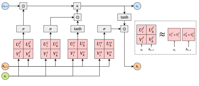
Figure 1: Factorized LSTM Cell

3.1 Long-Short Term Memory Networks

Long-Short Term Memory (LSTMs) networks are parameterized with two large matrices, $\mathbf{W}_{i}$, and $\mathbf{W}_{h}$. LSTM captures long-term dependencies in the input and avoids the exploding/vanishing gradient problems on the standard RNN. The gating layers control the information flow within the network and decide which information to keep, discard, or update in the memory. The following recurrent equations show the LSTM dynamics:

$$\small\begin{pmatrix}\mathbf{i}_{t}\\ \mathbf{f}_{t}\\ \mathbf{o}_{t}\\ \mathbf{\hat{c}}_{t}\end{pmatrix}=\begin{pmatrix}\sigma\\ \sigma\\ \sigma\\ \text{tanh}\end{pmatrix}\begin{pmatrix}\mathbf{W}_{i}&\mathbf{W}_{h}\end{pmatrix}\begin{pmatrix}\mathbf{x}_{t}\\ \mathbf{h}_{t-1}\end{pmatrix},$$ (1)

$$\small\mathbf{W}_{i}=\begin{pmatrix}\mathbf{W}_{i}^{i}\\ \mathbf{W}_{i}^{f}\\ \mathbf{W}_{i}^{o}\\ \mathbf{W}_{i}^{c}\end{pmatrix},\mathbf{W}_{h}=\begin{pmatrix}\mathbf{W}_{h}^{i}\\ \mathbf{W}_{h}^{f}\\ \mathbf{W}_{h}^{o}\\ \mathbf{W}_{h}^{c}\end{pmatrix},$$ (2)

$$\mathbf{c}_{t}= ~{}\mathbf{f}_{t}\odot\mathbf{c}_{t-1}+\mathbf{i}_{t}\odot\mathbf{\hat{c}}_{t},$$ (3)

$$\mathbf{h}_{t}= ~{}\mathbf{o}_{t}\odot\text{tanh}(\mathbf{c}_{t}).$$

where $\mathbf{x}_{t}\in\mathbb{R}^{n_{inp}}$, and $\mathbf{h}_{t}\in\mathbb{R}^{n_{dim}}$ at time $t$. Here, $\sigma(\cdot)$ and $\odot$ denote the sigmoid function and element-wise multiplication operator, respectively. The model parameters can be summarized in a compact form with: $\Theta=[\mathbf{W}_{i},\mathbf{W}_{h}]$, where $\mathbf{W}_{i}\in\mathbb{R}^{4*n_{inp}\times 4*n_{dim}}$ which is the input matrix, and $\mathbf{W}_{h}\in\mathbb{R}^{4*n_{dim}\times 4*n_{dim}}$ which is the hidden matrix. Note that we often refer $\mathbf{W}_{i}$ as additive recurrence and $\mathbf{W}_{h}$ as multiplicative recurrence, following terminology of [Levy et al., 2018].

3.2 Low-Rank Matrix Factorization

We consider two Low-Rank Matrix Factorization for LSTM compression: Truncated Singular Value Decomposition (SVD) and Semi Non-negative Matrix Factorization (Semi-NMF). Both methods factorize a matrix $\mathbf{W}$ into two matrices $\mathbf{U}_{m\times r}$ and $\mathbf{V}_{r\times n}$ such that $\mathbf{W}=\mathbf{U}\mathbf{V}$ [Fazel, 2002]. SVD produces a factorization by applying orthogonal constraints on the $\mathbf{U}$ and $\mathbf{V}$ factors along with an additional diagonal matrix of singular values, where instead Semi-NMF generalizes Non-negative Matrix Factorization (NMF) by relaxing some of the sign constraints on negative values for $\mathbf{U}$ and $\mathbf{W}$. The computation advantage, compared to pruning methods which require a special implementation of sparse matrix multiplication, is that the matrix $\boldsymbol{\mathbf{W}}$ requires $mn$ parameters and $mn$ flops, while $\mathbf{U}$ and $\mathbf{V}$ require $rm+rn=r(m+n)$ parameters and $r(m+n)$ flops. If we take the rank to be very low $r<<m,n$, the number of parameters in $\mathbf{U}$ and $\mathbf{V}$ is much smaller compared to $\mathbf{W}$.

As elaborated in Equation 1, a basic LSTM cell includes four gates: input, forget, output, and cell state, performing a linear combination on input at time $t$ and hidden state at time $t-1$. We propose to replace $\mathbf{W}_{i},\,\mathbf{W}_{h}$ pair for each gate with their low-rank decomposition, either SVD or Semi-NMF [Ding et al., 2010], leading to a significant reduction in memory and computational cost requirement. The general objective function is given as:

$$\underset{m\times n}{\mathbf{W}}=\underset{m\times r}{\mathbf{U}}\quad\underset{r\times n}{\mathbf{V}},$$ (4)

$$\underset{U,V}{\text{minimize}}\quad||\mathbf{W}-\mathbf{U}\mathbf{V}||_{F}^{2}.$$ (5)

3.3 Truncated Singular Value Decomposition (SVD)

One of the constrained matrix factorization method is based on Singular Value Decomposition (SVD) which produces a factorization by applying orthogonal constraints on the $\mathbf{U}$ and $\mathbf{V}$ factors. These approaches aim to find a linear combination of the basis vectors which restrict to the orthogonal vectors in feature space that minimize reconstruction error. In the case of the SVD, there are no restrictions on the signs of $\mathbf{U}$ and $\mathbf{V}$ factors. Moreover, the data matrix $\mathbf{W}$ is also unconstrained.

$$\mathbf{W}=\mathbf{U}\mathbf{S}\mathbf{V},$$ (6)

$$\underset{\mathbf{U},\mathbf{S},\mathbf{V}}{\text{minimize}}\quad||\mathbf{W}-\mathbf{U}\mathbf{S}\mathbf{V}||_{F}^{2}.$$ (7)

s.t. $\mathbf{U}$ and $\mathbf{V}$ are orthogonal, and $\mathbf{S}$ is diagonal. The optimal values $\mathbf{U}_{m\times r}^{r}$, $\mathbf{S}_{r\times r}^{r}$, $\mathbf{V}_{r\times n}^{r}$ for $\mathbf{U}_{m\times n}$, $\mathbf{S}_{n\times n}$, and $\mathbf{V}_{n\times n}$ are obtained by taking the top $r$ singular values from the diagonal matrix $\mathbf{S}$ and the corresponding singular vectors from $\mathbf{U}$ and $\mathbf{V}$.

3.4 Semi-NMF

Semi-NMF generalizes Non-negative Matrix Factorization (NMF) by relaxing some of the sign constraints on negative values for $\mathbf{U}$ and $\mathbf{W}$ ($\mathbf{V}$ has to be kept positive). Semi-NMF is more preferable in application to Neural Networks because of this generic capability of having negative values. To elaborate, when the input matrix $\mathbf{W}$ is unconstrained (i.e., contains mixed signs), we consider a factorization, in which we restrict $\mathbf{V}$ to be non-negative, while having no restriction on the signs of $\mathbf{U}$. We minimize the objective function as in Equation 8.

$$\mathbf{W}_{\pm}\approx\mathbf{U}_{\pm}\mathbf{V}_{+},$$ (8)

$$\underset{\mathbf{U},\mathbf{V}}{\text{minimize}}\quad||\mathbf{W}-\mathbf{U}\mathbf{V}||_{F}^{2}\quad\text{s.t. }\mathbf{V}\geq 0.$$ (9)

The optimization algorithm iteratively alternates between the update of $\mathbf{U}$ and $\mathbf{V}$ using coordinate descent [Luo and Tseng, 1992].

3.5 Pruning

We use the pruning methodology used in LSTMs from [Han et al., 2015] and [See et al., 2016b]. To elaborate, for each weight matrix $\mathbf{W}_{i,h}$, we mask the low-magnitude weights to zero, according to the compression ratio of the low-rank factorization.

Table 1: The table shows the total parameters, perplexity, and compression efficiency (lower is better) on PTB Language Modeling task. $\ddagger$ We reproduced the results.

PTB	Param.	w/o fine-tuning		w/ fine-tuning
		PPL	E(r)	PPL	E(r)
AWD-LSTM	24M	58.3‡	-	57.3	-
TT-LSTM	12M	168.6	2.92†	-	-
Semi-NMF $\mathbf{W}_{h}$ (r=10)	9M	78.5	0.72	58.11	-0.02
SVD $\mathbf{W}_{h}$ (r=10)	9M	78.07	0.32	58.18	-0.02
Pruning $\mathbf{W}_{h}$ (r=10)	9M	83.62	0.89	57.94	-0.03
Semi-NMF $\mathbf{W}_{h}$ (r=400)	18M	59.7	0.05	57.84	-0.02
SVD $\mathbf{W}_{h}$ (r=400)	18M	59.34	0.006	57.81	-0.02
Pruning $\mathbf{W}_{h}$ (r=400)	18M	59.47	0.03	57.19	-0.04
Semi-NMF $\mathbf{W}_{i}$ (r=10)	15M	485.4	19.81	81.4	1.04
SVD $\mathbf{W}_{i}$ (r=10)	15M	462.19	6.83	88.12	1.35
Pruning $\mathbf{W}_{i}$ (r=10)	15M	676.76	28.69	82.23	1.08
Semi-NMF $\mathbf{W}_{i}$ (r=400)	20M	62.7	0.42	58.47	-0.01
SVD $\mathbf{W}_{i}$ (r=400)	20M	60.59	0.02	58.04	-0.01
Pruning $\mathbf{W}_{i}$ (r=400)	20M	59.62	0.10	57.65	-0.02

Table 2: The table shows the total parameters, perplexity, and compression efficiency (lower is better) on WT-2 Language Modeling task. $\ddagger$ We reproduced the results.

WT-2	Params	PPL	E(r)
AWD-LSTM	24M	65.67‡	-
Semi-NMF $\mathbf{W}_{h}$ (r=10)	9M	102.17	65.14
SVD $\mathbf{W}_{h}$ (r=10)	9M	99.92	62.49
Pruning $\mathbf{W}_{h}$ (r=10)	9M	109.16	72.64
Semi-NMF $\mathbf{W}_{h}$ (r=400)	18M	66.5	4.33
SVD $\mathbf{W}_{h}$ (r=400)	18M	66.1	2.28
Pruning $\mathbf{W}_{h}$ (r=400)	18M	66.23	2.94
Semi-NMF $\mathbf{W}_{i}$ (r=10)	15M	481.61	197.57
SVD $\mathbf{W}_{i}$ (r=10)	15M	443.49	194.89
Pruning $\mathbf{W}_{i}$ (r=10)	15M	856.87	211.23
Semi-NMF $\mathbf{W}_{i}$ (r=400)	20M	68.41	22.68
SVD $\mathbf{W}_{i}$ (r=400)	20M	67.11	12.18
Pruning $\mathbf{W}_{i}$ (r=400)	20M	66.37	5.97

Table 3: The table shows the Accuracy/F1 with ELMo.

SST-5	r=10		r=400		Best
	Acc.	E(r)	Acc.	E(r)	Acc. (avg)	E(r) (avg)
BCN	-	-	-	-	53.7‡	-
BCN + ELMo	-	-	-	-	54.5‡	-
Semi-NMF $\mathbf{W}_{h}$	50.18	0.29	53.93	0.21	54.16 (52.93)	0.09 (0.17)
SVD $\mathbf{W}_{h}$	50.4	0.27	54.11	0.13	54.11 (52.84)	0.12 (0.17)
Pruning $\mathbf{W}_{h}$	50.81	0.25	54.66	-0.03	54.88 (53.59)	-0.07 (0.06)
Semi-NMF $\mathbf{W}_{i}$	38.23	1.1	54.11	0.15	54.11 (50.56)	0.12 (0.34)
SVD $\mathbf{W}_{i}$	40.58	0.94	54.34	0.05	54.38 (51.19)	0.02 (0.26)
Pruning $\mathbf{W}_{i}$	34.57	1.35	54.61	-0.01	54.66 (50.01)	-0.02 (0.33)

SNLI	r=10		r=400		Best
	Acc.	E(r)	Acc.	E(r)	Acc. (avg)	E(r) (avg)
ESIM	-	-	-	-	88.6	-
ESIM + ELMo	-	-	-	-	88.5‡	-
Semi-NMF $\mathbf{W}_{h}$	87.24	0.04	88.45	0.01	88.47 (88.18)	0.003 (0.01)
SVD $\mathbf{W}_{h}$	87.27	0.04	88.46	0.005	88.46 (88.18)	0.003 (0.01)
Pruning $\mathbf{W}_{h}$	87.51	0.03	88.53	-0.003	88.53 (88.23)	-0.003 (0.01)
Semi-NMF $\mathbf{W}_{i}$	77.08	0.39	88.44	0.01	88.44 (86.59)	0.01 (0.07)
SVD $\mathbf{W}_{i}$	78.15	0.35	88.48	0.002	88.48 (86.77)	0.007 (0.06)
Pruning $\mathbf{W}_{i}$	73.67	0.5	88.48	0.005	88.5 (85.8)	0.001 (0.09)

SQuAD	r=10		r=400		Best
	F1	E(r)	F1	E(r)	F1 (avg)	E(r) (avg)
BiDAF	-	-	-	-	77.3‡	-
BiDAF + ELMo	-	-	-	-	81.75‡	-
Semi-NMF $\mathbf{W}_{h}$	76.59	0.21	81.55	0.04	81.55 (80.32)	0.03 (0.07)
SVD $\mathbf{W}_{h}$	76.72	0.21	81.62	0.027	81.62 (80.47)	0.02 (0.06)
Pruning $\mathbf{W}_{h}$	52.02	0.49	81.73	0.006	81.65 (80.6)	0.006 (0.05)
Semi-NMF $\mathbf{W}_{i}$	60.69	0.88	81.78	-0.0003	81.78 (77.93)	-0.0003 (0.17)
SVD $\mathbf{W}_{i}$	57.14	1.03	81.78	-0.0003	81.78 (77.69)	-0.0003 (0.17)
Pruning $\mathbf{W}_{i}$	52.02	1.24	81.73	0.004	81.73 (76.06)	0.004 (0.25)

4 Evaluation

We evaluate using five different publicly available datasets spanning two domains: 1) Perplexity in two different Language Modeling (LM) datasets, 2) Accuracy/F1 in three downstream NLP tasks that ELMo achieved the state-of-the-art single-model performance. We also report the number of parameters, efficiency $E(r)$ (ratio of loss in performance to parameters compression), and inference time  in test set.

We benchmark the LM capability using Penn Treebank [Marcus et al., 1993, PTB] and WikiText-2 [Merity et al., 2017, WT2]. For the downstream NLP tasks, we evaluate our method in the Stanford Question Answering Dataset [Rajpurkar et al., 2016, SQuAD] the Stanford Natural Language Inference [Bowman et al., 2015, SNLI] corpus, and the Stanford Sentiment Treebank [Socher et al., 2013, SST-5] dataset.

For all datasets, we run experiments across different levels of low-rank approximation r with Semi-NMF and SVD, averaged over 5 runs, and compare with Pruning with same compression ratio. We also compare the factorization efficiency when only one of $\mathbf{W}_{i}$ or $\mathbf{W}_{h}$ was factorized. This is done in order to see which recurrence type (additive or multiplicative) is more suitable for compression.

4.1 Measure

For evaluating the performance of the compression we define efficiency measure as:

$$E(r)=\frac{R(M,M^{r})}{R(P,P^{r})}$$ (10)

where $M$ represent any evaluation metric (i.e. Accuracy, F1-score, Perplexity), $P$ represents the number of parameters, and $R(a,b)=\frac{a-b}{a}$ where $a=max(a,b)$, i.e. the ration. This indicator shows the ratio of loss in performance versus the loss in number of parameter. Hence, an efficient compression holds a very small $E$ since the denominator, $P-P^{r}$, became large just when the number of parameter decreases, and the numerator, $M-M^{r}$, became small only if there is no loss in the considered measure. In some cases $E$ became negative if there is an improvement.

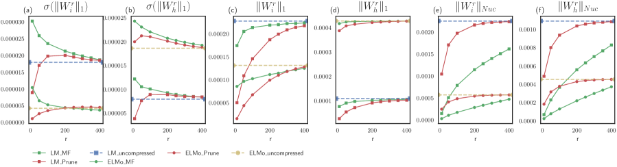
Figure 2: Norm analysis comparisons between MF and Pruning in Language Modeling (PTB) and ELMo. Rank versus (a) $\sigma(\|\mathbf{W}_{i}\|_{1})$ (b) $\sigma(\|\mathbf{W}_{h}\|_{1})$ (c) $\|\mathbf{W}_{i}\|_{1}$ (d) $\|\mathbf{W}_{h}\|_{1}$ (e) $\|\mathbf{W}_{i}\|_{Nuc}$ (f) $\|\mathbf{W}_{h}\|_{Nuc}$.

4.2 Language Modeling (LM)

We train a 3-layer LSTM Language Model proposed by [Merity et al., 2018], following the same training details for both datasets, using their released code . In PTB, we fine-tune the compressed model for several epochs. Table 1 reports the perplexity among different ranks in $\mathbf{W}_{i,h}$. It is clear that compressing $\mathbf{W}_{h}$ works notably better than $\mathbf{W}_{i}$. We achieve similar results for WT-2. In general, SVD has the lowest perplexity among others. This difference becomes more evident for higher compression (e.g., r=10). Moreover, all the methods perform better than the result reported by [Grachev et al., 2017] using Tensor Train (TT-LSTM). Using fine-tuning with rank 10 all the methods we achieve a small improvement compared to the baseline with a 2.13x speedup.

4.3 NLP Tasks with ELMo

To highlight the practicality of our proposed method, we also measure the factorization performances with models using pre-trained ELMo [Peters et al., 2018], as ELMo is essentially a 2-layer bidirectional LSTM Language Model that captures rich contextualized representations. Using the same publicly released pre-trained ELMo weights  as the input embedding layer of all three tasks, we train publicly available state-of-the-art models as in [Peters et al., 2018]: BiDAF [Seo et al., 2016] for SQuAD, ESIM [Chen et al., 2017] for SNLI, and BCN [McCann et al., 2017] for SST-5. Similar to the Language Modeling tasks, we low-rank factorize the pre-trained ELMo layer only, and compare the accuracy and F1 scores across different levels of low-rank approximation. Note that although many of these models are based on RNNs, we factorize only the ELMo layer in order to show that our approach can effectively compress pre-trained transferable knowledge. As we only compress the ELMo weights, and other layers of each model also have large number of parameters, the inference time is affected less than in Language Modeling tasks. The percentage of parameters in the ELMo layer for BiDAF (SQuAD) is 59.7%, for ESIM (SNLI) 67.4%, and for BCN (SST-5) 55.3%.

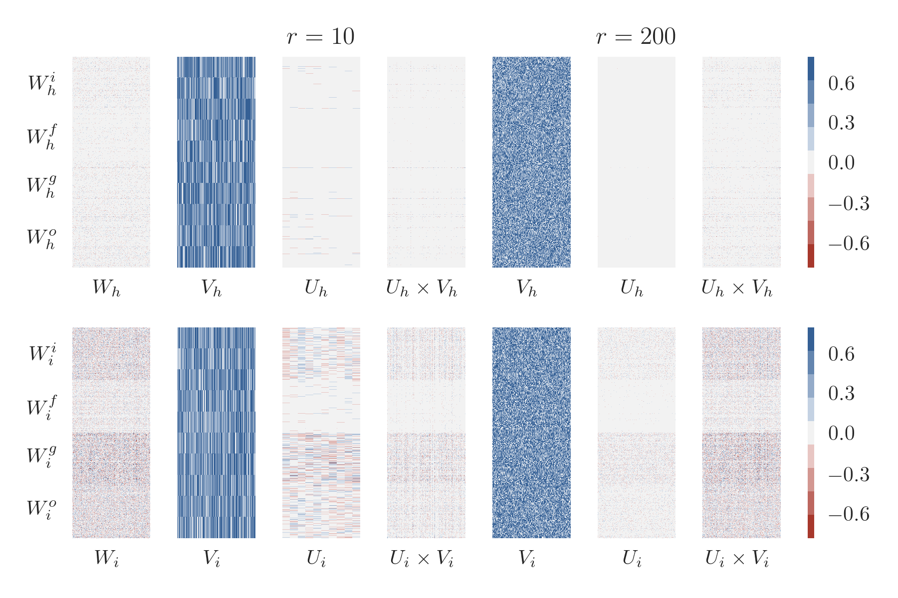
Figure 3: Heatmap LSTM weights on PTB.

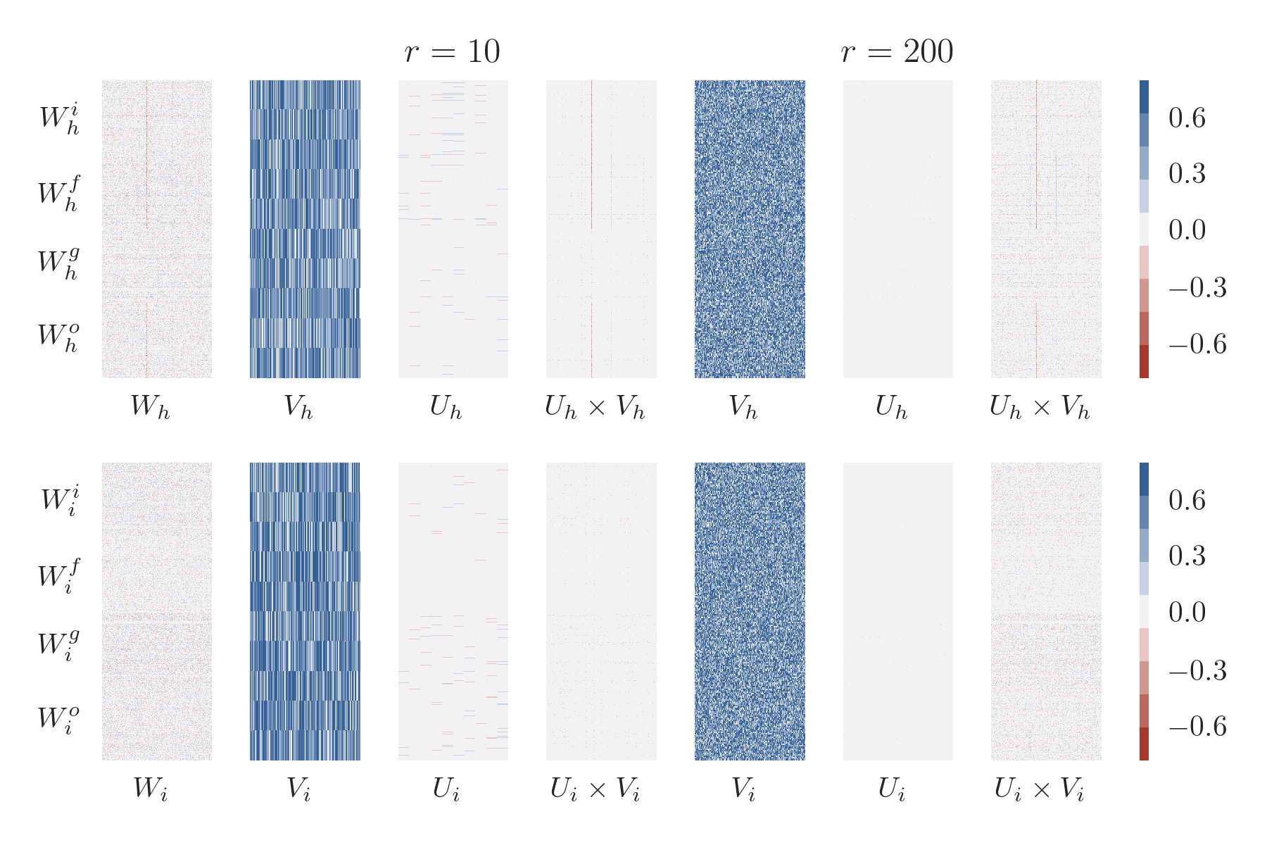
Figure 4: Heatmap of ELMo forward weights.

From Table 3, for SST-5 and SNLI, we can see that compressing $\mathbf{W}_{h}$ is in general more efficient and better performing than compressing $\mathbf{W}_{i}$, except for SVD in SST-5. On the other hand, for the results on SQuAD, Table 3 shows the opposite trend, in which compressing $\mathbf{W}_{i}$ constantly outperforms compressing $\mathbf{W}_{h}$ for all methods we experimented with. In fact, we can see that, in average, using highly compressed ELMo with BiDAF still performs better than without. Overall, we can see that for all datasets, we achieve performances that are not significantly different from the baseline results even after compressing over more than 10M parameters.

4.4 Norm Analysis

In the previous section, we observe two interesting points: 1) Matrix Factorization (MF) works consistently better in PTB and Wiki-Text 2, but Pruning works better in ELMo for $\mathbf{W}_{h}$, 2) Factorizing $\mathbf{W}_{h}$ is generally better than factorizing $\mathbf{W}_{i}$. To answer these questions, we collect the L1 norm and Nuclear norm statistics, defined in Figure 2, comparing among $\mathbf{W}_{h}$ and $\mathbf{W}_{i}$ for both PTB and ELMo. L1 and its standard deviation (std) together describe the sparsity of a matrix, and Nuclear norm approximates the matrix rank.

MF versus Pruning in $\mathbf{W}_{i}$

From the results, we observe that MF performs better than Pruning in compressing $\mathbf{W}_{i}$ for high compression ratios. Figure 2 shows rank $r$ versus L1 norm and its standard deviation, in both PTB and ELMo. The first notable pattern from Figure 2 Panel (a) is that MF and Pruning have diverging values from $r\leq 200$. We can see that Pruning makes the std of L1 lower than the uncompressed, while MF monotonically increases the std from uncompressed baseline. This means that as we approximate to lower ranks ($r\leq 200$), MF retains more salient information, while Pruning loses some of that salient information. This can be clearly shown from Panel (c), in which Pruning always drops significantly more in L1 than MF does.

MF versus Pruning in $\mathbf{W}_{h}$

The results for $\mathbf{W}_{h}$ are also consistent in both PTB and WT2; MF works better than Pruning for higher compression ratios. On the other hand, results from Table 3 show that Pruning works better than MF in $\mathbf{W}_{h}$ of ELMo even in higher compression ratios.

We can see from Panel (d) that L1 norms of MF and Pruning do not significantly deviate nor decrease much from the uncompressed baseline. Meanwhile, Panel (b) reveals an interesting pattern, in which the std actually increases for Pruning and is always kept above the uncompressed baseline. This means that Pruning retains salient information for $\mathbf{W}_{h}$, while keeping the matrix sparse.

This behavior of $\mathbf{W}_{h}$ can be explained by the nature of the compression and with inherent matrix sparsity. In this setting, pruning is zeroing values already close to zero, so it is able to keep the L1 stable while increasing the std. On the other hand, MF instead reduces noise by pushing lower values to be even lower (or zero) and keeps salient information by pushing larger values to be even larger. This pattern is more evident in Figure 3 and Figure 4, in which you can see a clear salient red line in $\mathbf{W}_{h}$ that gets even stronger after factorization ($\mathbf{U}_{h}\times\mathbf{V}_{h}$). Naturally, when the compression rate is low (e.g., r=300) pruning is more efficient strategy then MF.

$\mathbf{W}_{i}$ versus $\mathbf{W}_{h}$

We show the change in Nuclear norm and their corresponding starting points (i.e., uncompressed) in Figure 2 Panels (e) and (f). Notably, $\mathbf{W}_{h}$ has a consistently lower nuclear norm in both tasks compared to $\mathbf{W}_{i}$. This difference is larger for LM (PTB), in which $\|\mathbf{W}_{i}\|_{Nuc}$ is twice of that of $\|\mathbf{W}_{h}\|_{Nuc}$. By definition, having a lower nuclear norm is often an indicator of low-rank in a matrix; hence, we hypothesize that $\mathbf{W}_{h}$ is inherently low-rank than $\mathbf{W}_{i}$. We confirm this from Panel (d), in which even with a very high compression ratio (e.g., $r=10$), the L1 norm does not decrease that much. This explains the large gap in performance between the compression of $\mathbf{W}_{i}$ and $\mathbf{W}_{h}$. On the other hand, in ELMo, this gap in norm is lower and also shows smaller differences in performance between $\mathbf{W}_{i}$ and $\mathbf{W}_{h}$, and also sometimes even the opposite in SQuAD. Hence, we believe that smaller nuclear norms lead to better performance for all compression methods.

5 Conclusion

In conclusion, we empirically verified the limits of compressing LSTM gates using low-rank matrix factorization and pruning in four different NLP tasks. Our experiment results and norm analysis show that Low-Rank Matrix Factorization works better in general than pruning, except for particularly sparse matrices. We also discover that inherent low-rankness and low nuclear norm correlate well, explaining why compressing multiplicative recurrence works better than compressing additive recurrence. In future works, we plan to factorize all LSTMs in the model, e.g. BiDAF model, and try to combine both Pruning and Matrix Factorization.

References

- [Bahdanau et al., 2014] Dzmitry Bahdanau, Kyunghyun Cho, and Yoshua Bengio. 2014. Neural machine translation by jointly learning to align and translate. arXiv preprint arXiv:1409.0473.
- [Belletti et al., 2018] Francois Belletti, Alex Beutel, Sagar Jain, and Ed Chi. 2018. Factorized recurrent neural architectures for longer range dependence. In International Conference on Artificial Intelligence and Statistics, pages 1522–1530.
- [Bowman et al., 2015] Samuel R. Bowman, Gabor Angeli, Christopher Potts, and Christopher D. Manning. 2015. A large annotated corpus for learning natural language inference. In Proceedings of the 2015 Conference on Empirical Methods in Natural Language Processing (EMNLP). Association for Computational Linguistics.
- [Chen et al., 2017] Qian Chen, Xiaodan Zhu, Zhen-Hua Ling, Si Wei, Hui Jiang, and Diana Inkpen. 2017. Enhanced lstm for natural language inference. In Proceedings of the 55th Annual Meeting of the Association for Computational Linguistics (Volume 1: Long Papers), volume 1, pages 1657–1668.
- [Denil et al., 2013] Misha Denil, Babak Shakibi, Laurent Dinh, Nando De Freitas, et al. 2013. Predicting parameters in deep learning. In Advances in neural information processing systems, pages 2148–2156.
- [Ding et al., 2010] Chris HQ Ding, Tao Li, and Michael I Jordan. 2010. Convex and semi-nonnegative matrix factorizations. IEEE transactions on pattern analysis and machine intelligence, 32(1):45–55.
- [Fan et al., 2014] Hao-Teng Fan, Jeih-weih Hung, Xugang Lu, Syu-Siang Wang, and Yu Tsao. 2014. Speech enhancement using segmental nonnegative matrix factorization. In Acoustics, Speech and Signal Processing (ICASSP), 2014 IEEE International Conference on, pages 4483–4487. IEEE.
- [Fazel, 2002] Maryam Fazel. 2002. Matrix rank minimization with applications. Ph.D. thesis, PhD thesis, Stanford University.
- [Geiger et al., 2014] Jürgen T Geiger, Jort F Gemmeke, Björn Schuller, and Gerhard Rigoll. 2014. Investigating nmf speech enhancement for neural network based acoustic models. In Proc. INTERSPEECH 2014, ISCA, Singapore, Singapore.
- [Gers et al., 2000] Felix A. Gers, Jürgen A. Schmidhuber, and Fred A. Cummins. 2000. Learning to forget: Continual prediction with lstm. Neural Comput., 12(10):2451–2471, October.
- [Gong et al., 2014] Yunchao Gong, Liu Liu, Ming Yang, and Lubomir Bourdev. 2014. Compressing deep convolutional networks using vector quantization. arXiv preprint arXiv:1412.6115.
- [Grachev et al., 2017] Artem M Grachev, Dmitry I Ignatov, and Andrey V Savchenko. 2017. Neural networks compression for language modeling. In International Conference on Pattern Recognition and Machine Intelligence, pages 351–357. Springer.
- [Han et al., 2015] Song Han, Jeff Pool, John Tran, and William Dally. 2015. Learning both weights and connections for efficient neural network. In C. Cortes, N. D. Lawrence, D. D. Lee, M. Sugiyama, and R. Garnett, editors, Advances in Neural Information Processing Systems 28, pages 1135–1143. Curran Associates, Inc.
- [Han et al., 2016] Song Han, Huizi Mao, and William J Dally. 2016. Deep compression: Compressing deep neural networks with pruning, trained quantization and huffman coding. ICLR.
- [He et al., 2017] Luheng He, Kenton Lee, Mike Lewis, and Luke Zettlemoyer. 2017. Deep semantic role labeling: What works and what’s next. In Proceedings of the 55th Annual Meeting of the Association for Computational Linguistics (Volume 1: Long Papers), volume 1, pages 473–483.
- [Hinton et al., 2015] Geoffrey Hinton, Oriol Vinyals, and Jeff Dean. 2015. Distilling the knowledge in a neural network. stat, 1050:9.
- [Hochreiter and Schmidhuber, 1997] Sepp Hochreiter and Jürgen Schmidhuber. 1997. Long short-term memory. Neural computation, 9(8):1735–1780.
- [Hong et al., 2016] Seunghoon Hong, Jonghyun Choi, Jan Feyereisl, Bohyung Han, and Larry S Davis. 2016. Joint image clustering and labeling by matrix factorization. IEEE transactions on pattern analysis and machine intelligence, 38(7):1411–1424.
- [Huang et al., 2018] Qiangui Huang, Kevin Zhou, Suya You, and Ulrich Neumann. 2018. Learning to prune filters in convolutional neural networks. arXiv preprint arXiv:1801.07365.
- [Jaderberg et al., 2014] Max Jaderberg, Andrea Vedaldi, and Andrew Zisserman. 2014. Speeding up convolutional neural networks with low rank expansions. In Proceedings of the British Machine Vision Conference. BMVA Press.
- [James Bradbury and Socher, 2017] Caiming Xiong James Bradbury, Stephen Merity and Richard Socher. 2017. Quasi-recurrent neural networks. In International Conference on Learning Representations.
- [Kuchaiev and Ginsburg, 2017] Oleksii Kuchaiev and Boris Ginsburg. 2017. Factorization tricks for lstm networks. ICLR Workshop.
- [Lee et al., 2017] Kenton Lee, Luheng He, Mike Lewis, and Luke Zettlemoyer. 2017. End-to-end neural coreference resolution. In Proceedings of the 2017 Conference on Empirical Methods in Natural Language Processing, pages 188–197.
- [Levy et al., 2018] Omer Levy, Kenton Lee, Nicholas FitzGerald, and Luke Zettlemoyer. 2018. Long short-term memory as a dynamically computed element-wise weighted sum. In Proceedings of the 56th Annual Meeting of the Association for Computational Linguistics (Volume 2: Short Papers), pages 732–739. Association for Computational Linguistics.
- [Li et al., 2017] Xuelong Li, Guosheng Cui, and Yongsheng Dong. 2017. Graph regularized non-negative low-rank matrix factorization for image clustering. IEEE transactions on cybernetics, 47(11):3840–3853.
- [Liu et al., 2018] Xuan Liu, Di Cao, and Kai Yu. 2018. Binarized lstm language model. In Proceedings of the 2018 Conference of the North American Chapter of the Association for Computational Linguistics: Human Language Technologies, Volume 1 (Long Papers), pages 2113–2121. Association for Computational Linguistics.
- [Lu et al., 2016] Zhiyun Lu, Vikas Sindhwani, and Tara N Sainath. 2016. Learning compact recurrent neural networks. In Acoustics, Speech and Signal Processing (ICASSP), 2016 IEEE International Conference on, pages 5960–5964. IEEE.
- [Luo and Tseng, 1992] Zhi-Quan Luo and Paul Tseng. 1992. On the convergence of the coordinate descent method for convex differentiable minimization. Journal of Optimization Theory and Applications, 72(1):7–35.
- [Marcus et al., 1993] Mitchell P. Marcus, Mary Ann Marcinkiewicz, and Beatrice Santorini. 1993. Building a large annotated corpus of english: The penn treebank. Comput. Linguist., 19(2):313–330, June.
- [McCann et al., 2017] Bryan McCann, James Bradbury, Caiming Xiong, and Richard Socher. 2017. Learned in translation: Contextualized word vectors. In Advances in Neural Information Processing Systems, pages 6294–6305.
- [Melis et al., 2018] Gábor Melis, Chris Dyer, and Phil Blunsom. 2018. On the state of the art of evaluation in neural language models. In International Conference on Learning Representations.
- [Merity et al., 2017] Stephen Merity, Caiming Xiong, James Bradbury, and Richard Socher. 2017. Pointer sentinel mixture models. ICLR.
- [Merity et al., 2018] Stephen Merity, Nitish Shirish Keskar, and Richard Socher. 2018. Regularizing and optimizing LSTM language models. In International Conference on Learning Representations.
- [Miceli Barone, 2018] Antonio Valerio Miceli Barone. 2018. Low-rank passthrough neural networks. In Proceedings of the Workshop on Deep Learning Approaches for Low-Resource NLP, pages 77–86. Association for Computational Linguistics.
- [Mikolov, 2012] Tomáš Mikolov. 2012. Statistical language models based on neural networks. Presentation at Google, Mountain View, 2nd April.
- [Mohammadiha et al., 2013] Nasser Mohammadiha, Paris Smaragdis, and Arne Leijon. 2013. Supervised and unsupervised speech enhancement using nonnegative matrix factorization. IEEE Transactions on Audio, Speech, and Language Processing, 21(10):2140–2151.
- [Oseledets, 2011] Ivan V Oseledets. 2011. Tensor-train decomposition. SIAM Journal on Scientific Computing, 33(5):2295–2317.
- [Peters et al., 2018] Matthew Peters, Mark Neumann, Mohit Iyyer, Matt Gardner, Christopher Clark, Kenton Lee, and Luke Zettlemoyer. 2018. Deep contextualized word representations. In Proceedings of the 2018 Conference of the North American Chapter of the Association for Computational Linguistics: Human Language Technologies, Volume 1 (Long Papers), pages 2227–2237. Association for Computational Linguistics.
- [Rajpurkar et al., 2016] Pranav Rajpurkar, Jian Zhang, Konstantin Lopyrev, and Percy Liang. 2016. Squad: 100,000+ questions for machine comprehension of text. In Proceedings of the 2016 Conference on Empirical Methods in Natural Language Processing, pages 2383–2392. Association for Computational Linguistics.
- [See et al., 2016a] Abigail See, Minh-Thang Luong, and Christopher D Manning. 2016a. Compression of neural machine translation models via pruning. CoNLL 2016, page 291.
- [See et al., 2016b] Abigail See, Minh-Thang Luong, and Christopher D. Manning. 2016b. Compression of neural machine translation models via pruning. In Proceedings of The 20th SIGNLL Conference on Computational Natural Language Learning, pages 291–301. Association for Computational Linguistics.
- [Seo et al., 2016] Minjoon Seo, Aniruddha Kembhavi, Ali Farhadi, and Hannaneh Hajishirzi. 2016. Bidirectional attention flow for machine comprehension. ICLR 2017.
- [Socher et al., 2013] Richard Socher, Alex Perelygin, Jean Wu, Jason Chuang, Christopher D. Manning, Andrew Ng, and Christopher Potts. 2013. Recursive deep models for semantic compositionality over a sentiment treebank. In Proceedings of the 2013 Conference on Empirical Methods in Natural Language Processing, pages 1631–1642. Association for Computational Linguistics.
- [Sundermeyer et al., 2012] Martin Sundermeyer, Ralf Schlüter, and Hermann Ney. 2012. Lstm neural networks for language modeling. In Thirteenth Annual Conference of the International Speech Communication Association.
- [Sutskever et al., 2014] Ilya Sutskever, Oriol Vinyals, and Quoc V Le. 2014. Sequence to sequence learning with neural networks. In Advances in neural information processing systems, pages 3104–3112.
- [Tjandra et al., 2017] Andros Tjandra, Sakriani Sakti, and Satoshi Nakamura. 2017. Compressing recurrent neural network with tensor train. In Neural Networks (IJCNN), 2017 International Joint Conference on, pages 4451–4458. IEEE.
- [Trigeorgis et al., 2014] George Trigeorgis, Konstantinos Bousmalis, Stefanos Zafeiriou, and Bjoern Schuller. 2014. A deep semi-nmf model for learning hidden representations. In International Conference on Machine Learning, pages 1692–1700.
- [Wen et al., 2018] Wei Wen, Yuxiong He, Samyam Rajbhandari, Minjia Zhang, Wenhan Wang, Fang Liu, Bin Hu, Yiran Chen, and Hai Li. 2018. Learning intrinsic sparse structures within long short-term memory. In International Conference on Learning Representations.
- [Wilson et al., 2008] Kevin W Wilson, Bhiksha Raj, Paris Smaragdis, and Ajay Divakaran. 2008. Speech denoising using nonnegative matrix factorization with priors. In Acoustics, Speech and Signal Processing, 2008. ICASSP 2008. IEEE International Conference on, pages 4029–4032. IEEE.
- [Yang et al., 2017] Yinchong Yang, Denis Krompass, and Volker Tresp. 2017. Tensor-train recurrent neural networks for video classification. In International Conference on Machine Learning, pages 3891–3900.