Spreading speeds and traveling waves for monotone systems of impulsive reaction-diffusion equations: application to tree-grass interactions in fire-prone savannas

Abstract

Many systems in life sciences have been modeled by reaction-diffusion equations. However, under some circumstances, these biological systems may experience instantaneous and periodic perturbations (e.g. harvest, birth, release, fire events, etc) such that an appropriate formalism is necessary, using, for instance, impulsive reaction-diffusion equations. While several works tackled the issue of traveling waves for monotone reaction-diffusion equations and the computation of spreading speeds, very little has been done in the case of monotone impulsive reaction-diffusion equations. Based on vector-valued recursion equations theory, we aim to present in this paper results that address two main issues of monotone impulsive reaction-diffusion equations. First, they deal with the existence of traveling waves for monotone systems of impulsive reaction-diffusion equations. Second, they allow the computation of spreading speeds for monotone systems of impulsive reaction-diffusion equations. We apply our methodology to a planar system of impulsive reaction-diffusion equations that models tree-grass interactions in fire-prone savannas. Numerical simulations, including numerical approximations of spreading speeds, are finally provided in order to illustrate our theoretical results and support the discussion.

1 Introduction

In nature, all organisms migrate or disperse to some extent. This can take diverse forms such as walking, swimming, flying, or being transported by wind or flowing water, see Shigesada and Kawasaki Shigesada1997 . Such a migration, or dispersion, can be to some extent related to human activities that bring drastic changes in the global environment. According to Shigesada1997 , dispersive movements become noticeable when an offspring or a seed leaves its natal site, or when an organism’s habitat deteriorates from overcrowding. The spatially explicit ecological theories of such events have been made possible thanks to successful development of mathematical models that have played a central role in the description of migrations, see Friedman Friedman1964 , Shigesada and Kawasaki Shigesada1997 , Okubo and Levin Okubo2001 , Cantrell and Cosner Cantrell2003 , Volpert Volpert2014 , Logan Logan2008 , Logan2015 , Perthame Perthame2015 , and the references therein.

Mathematical literature dealing with the species’ spread mostly relies on reaction-diffusion equations that assume that the dispersal is governed by random diffusion and that it, along with the growth processes, take place continuously in time and space, (Cantrell and Cosner Cantrell2003 , Lewis and Li Lewis2012 ). This approach has had a remarkable success in explaining the rates at which species have invaded large open environments, see Shigesada and Kawasaki Shigesada1997 , Okubo and Levin Okubo2001 , Cantrell and Cosner Cantrell2003 , Lewis and Li Lewis2012 , Volpert Volpert2014 , Logan Logan2008 , Logan2015 , Perthame Perthame2015 . However, it is well-known that ecological species may experience several phenomena that, depending on circumstances, can be either time-continuous (growth, death, birth, release, etc.), or time-discrete (harvest, birth, death, release, etc.), see also Ma and Li Ma2009 , Dumont and Tchuenche Dumont2012 , Yatat et al. Yatat2017 , Yatat PhDYatatDjeumen2018 and the references therein. In the case of time-discrete perturbations, whose duration is negligible in comparison with the duration of the process, it is natural to assume that these perturbations act instantaneously; that is, in the form of impulses (Lakshmikantham et al. Lakshmikantham1989 , Bainov and Simeonov Bainov1995 ). Hence, there is a need to create a meaningful mathematical framework to analyse models leading to, say, impulsive reaction-diffusion equations.

Before going further, let us make some comments about how $\tau$-periodic impulsive phenomena are taken into account in mathematical models. Here, for simplicity of the exposition, we will focus on mathematical models depending only on time. We note that there exist several possibilities to model pulse events such as the formalism presented in (Lakshmikantham et al. Lakshmikantham1989 , Bainov and Simeonov Bainov1995 , Dumont and Tchuenche Dumont2012 , Dufourd and Dumont Dufourd2013 , Tchuinté Tamen et al. Tchuinte2016 , Tchuinte2017 , Yatat PhDYatatDjeumen2018 , Yatat et al. Yatat2017 , Yatat2018 and the references therein), or the approach used by Lewis and Li Lewis2012 , see also Weinberger et al. Weinberger2002 , Lewis et al. Lewis2002 , Li et al. Li2005 , Vasilyeva et al. Vasilyeva2016 , Fazly et al. Fazly2017 , Huang et al. Huang2017 , Yatat and Dumont YatatDumont2018 and the references therein.

Following Lakshmikantham1989 , we describe the evolution process by

$$\begin{array}[]{l}\displaystyle\frac{dx}{dt}=f(t,x),\quad t\neq k\tau,\\ \end{array}$$ (1)

$$\begin{array}[]{l}x(k\tau^{+})-x(k\tau^{-})=g(k\tau,x(k\tau^{-})),\quad k=1,2,3,...,\end{array}$$ (2)

where $f,g:\mathbb{R}_{+}\times\Omega\rightarrow\mathbb{R}^{n}$, $\Omega\subseteq\mathbb{R}^{n}$ is an open set and

$$x(k\tau^{\pm})=\lim\limits_{\theta\rightarrow 0}x(k\tau\pm\theta).$$

Usually, $x$ is assumed to be left-continuous; that is, $x(k\tau^{-})=x(k\tau)$. Let $x(t)=x(t,t_{0},x_{0})$ be any solution of (1) starting at $(t_{0},x_{0})$. The evolution process behaves as follows: the point $p_{t}=(t,x(t))$ begins its motion from the initial point $p_{t_{0}}=(t_{0},x_{0})$ and moves along the curve $\{(t,x):t\geq t_{0},x=x(t)\}$ until the time $t_{1}=\tau>t_{0}$ at which the point $p_{t_{1}}=(t_{1},x(t_{1}))$ is transferred to $p_{t_{1}^{+}}=(t_{1},x_{1}^{+})$ where $x_{1}^{+}=x(t_{1})+g(t_{1},x(t_{1}))$. Then the point $p_{t}$ continues to move further along the curve with $x(t)=x(t,t_{1},x_{1}^{+})$ as the solution of (1) starting at $p_{t_{1}}=(t_{1},x_{1}^{+})$ until the next moment $t_{2}=2\tau>t_{1}$. Then, once again the point $p_{t_{2}}=(t_{2},x(t_{2}))$ is transferred to $p_{t_{2}^{+}}=(t_{2},x_{2}^{+}),$ where $x_{2}^{+}=x(t_{2})+g(t_{2},x(t_{2}))$. As before, the point $p_{t}$ continues to move forward with $x(t)=x(t,t_{2},x_{2}^{+})$ as the solution of (1) starting at $(t_{2},x_{2}^{+})$. Thus, the evolution process continues forward as long as the solution of (1) exits.

To describe the other approach, we focus on $\tau$-periodic impulsive perturbations. The inter-perturbation season (i.e. the time between two successive perturbations) has length $\tau$ (units of time) and at the end of the inter-perturbation season, a prescribed perturbation occurs. Hence, we can consider the whole time interval as a succession of inter-perturbation seasons of length $\tau$. We denote the state variable at time $t\in[0,\tau]$ during the inter-perturbation season $k\in\mathbb{N}^{*}=\{1,2,3,...\}$ by $x_{k}(t)\in\mathbb{R}^{n};$ its inter-perturbation dynamics is described by

$$\begin{array}[]{l}\displaystyle\frac{dx_{k}}{dt}=f(t,x_{k}),\quad 0\leq t\leq\tau,\\ \end{array}$$ (3)

where $f:\mathbb{R}_{+}\times\Omega\rightarrow\mathbb{R}^{n}$ is a $\tau$-periodic function and $\Omega\subseteq\mathbb{R}^{n}$ is an open set. By the end of each season the perturbation is given by an updating condition

$$\begin{array}[]{l}x_{k+1}(0)=G_{k}[x_{k}(\tau)],\end{array}$$ (4)

where $G_{k}:\Omega\to\Omega,k=1,2,\ldots,$ are (possibly) nonlinear operators, with given $x_{1}(0)\in\Omega.$ Then system (3)-(4) can be written as

$$\begin{array}[]{l}x_{k+1}(0)=G_{k}Q[x_{k}(0)],\quad k=1,2,3,...\end{array}$$ (5)

where $Q$ is the so called time-$\tau$-map operator solution of system (3). We note that there are analytic links between these two formalisms, see YatatDumont2018 .

There are several works that considered the impact of impulsive perturbations on the dynamics of a system, both in the space-implicit and space-explicit case (see also Section 2). Very often, impulsive perturbations in space-implicit mathematical models result in the occurrence of periodic solutions in the model (e.g. Ma and Li Ma2009 , Yatat et al. Yatat2017 and references therein). For space-explicit impulsive mathematical models in bounded domains, in addition to periodic solutions that may occur, the issue of minimal domain has been also addressed (e.g. Lewis and Li Lewis2012 , Yatat and Dumont YatatDumont2018 ). On the other hand, in unbounded domains the problems of the existence of travelling wave solutions and the computation of the spreading speeds are hardly addressed (see below).

The study of traveling waves, as well as the computation of spreading speeds for monotone systems of reaction-diffusion equations, have been done by several authors (e.g. Weinberger et al. Weinberger2002 , Lewis et al. Lewis2002 , Li et al. Li2005 , Volpert Volpert2014 , Yatat et al. Yatat2017b and references therein). However, little is known about the case of impulsive reaction-diffusion equations. For a scalar impulsive reaction-diffusion equation, Yatat and Dumont YatatDumont2018 considered the Fisher-Kolmogorov-Petrowsky-Piscounov (FKPP) equation and obtained conditions under which an invasive traveling wave, connecting the extinction equilibrium and the positive equilibrium may exist (see also Lewis and Li Lewis2012 ). To the best of our knowledge, the existence of traveling waves for system of impulsive reaction-diffusion equation was studied only in Huang et al. Huang2017 , and only in a particular case. Precisely, the authors considered a stage-structured population model, were only one stage (or state variable) experiences a spatial diffusion, while the others are stationary. This assumption leads to a partially degenerate system of impulsive reaction-diffusion equations. Moreover, they also assumed reaction term for the diffusing state variable as linear.

The aim of this paper is to give some insights into the existence of traveling wave solutions for monotone systems of impulsive reaction-diffusion equations as well as the computation of their spreading speeds. Precisely, we use the vector-valued recursion theory proposed by Weinberger et al. Weinberger2002 (see also Lewis et al. Lewis2002 , Li et al. Li2005 , Lewis and Li Lewis2012 and the references therein) to develop a framework that is able to deal with the existence of traveling wave solutions for monotone systems of impulsive reaction-diffusion equations and the computation of spreading speeds. The paper is organized as follows: Section 2 deals with a brief review of both space-implicit and space-explicit mathematical models that take into account pulse events. Section 3 deals with the presentation of the framework for the computation of the spreading speeds and the existence of traveling wave solutions for monotone systems of impulsive reaction-diffusion equations. Section 4 deals with the application of this framework to a system of two impulsive reaction-diffusion equations that models tree-grass interactions in fire-prone savannas. We also provide some numerical illustrations of our theoretical results and, in particular, we show an approximation of the spreading speeds.

2 A brief review of mathematical models describing pulse events

We now provide a brief literature review of both space-implicit and space-explicit impulsive mathematical models.

2.1 Space-implicit impulsive models

Several types of perturbations, or instantaneous phenomena, have been considered as pulse events in mathematical models. These include events such as birth, vaccination, release, harvest, or fire events. The resulting impulsive models were rigorously analyzed by their authors by the well-known theory due to Lakshmikantham et al. Lakshmikantham1989 , Bainov and Simeonov Bainov1995 and Bainov1989 , or Lakmeche and Arino Lakmeche2000 . We note that, by using a suitable comparison argument, the standard theory of ordinary differential equations (Hale Hale1988 , Hale1980 ) can also be used.

2.1.1 Modelling births as pulse events

Several authors (Ma and Li Ma2009 , Wenjun and Jin Wenjun2007 , Zhang et al. Zhang2008 ) analysed the dynamics of infectious diseases in a population, where births occur periodically as a single pulse and also compared the effects of constant and pulse birth process. Namely, they found that if the birth pulse period is greater than some threshold that depends on the parameters related to the dynamics of the infection, then it is easier for such a population to eliminate the disease than if the birth process is constant. On the other hand, if the birth pulse period is lower than the threshold, then the population with a constant birth process eliminates the disease faster. In other words, when the birth pulse period gets very large, the births become less important and have little effect on the population. Hence, the disease in the population with a pulse birth can be eliminated more easily. However, as the birth pulse period gets very small, the population gives births many times in a very short time period, which have stronger effect on the population than in the case with constant births. Then it becomes more difficult to eradicate the disease in the populations with pulse births (Ma and Li Ma2009 ).

2.1.2 Modelling vaccinations as pulse events

Vaccination strategies are designed and applied to anticipate, control, or eradicate infectious diseases. Vaccination strategies include continuous-time vaccination and pulse vaccination. Pulse vaccination strategy (PVS) consists of periodic repetition of impulsive vaccinations in a population, for all the age cohorts. At each vaccination time, a constant fraction of susceptibles is vaccinated. This kind of vaccination is called impulsive since all the vaccine doses are applied in a time period which is very short with respect to the time scale of the target disease (Ma and Li Ma2009 ). The theoretic analysis of PVS was done by several authors and it was found that this strategy can keep the density of susceptible individuals always below some threshold above which the epidemics will be recurrent (Agur et al. Agur1993 ). In addition, they showed that PVS may allow for the eradication of the disease with a lower fraction of vaccinated susceptibles, than if the continuous-time vaccination strategy was applied (Agur et al. Agur1993 , Shulgin et al. Shulgin1998 , D’Onofrio Donofrio2002 , Zheng et al. Zheng2003 , Ma and Li Ma2009 and references therein).

2.1.3 Modelling releases as pulse events

In the framework of biological control of pests or vectors of infectious diseases, the sterile insect technique (SIT) is one of the promising ones. SIT control generally consists in massive releases of sterile insects in the targeted area in order to eliminate, or at least to lower the pest population under a certain threshold (Anguelov et al. Anguelov2019TIS ). Generally, SIT releases are done periodically. That is why several authors modelled the release process as a periodic impulsive event, while keeping the continuous-time differential equation framework for the birth, growth, death, or mating process (e.g. White et al. White2010 , Dumont and Tchuenche Dumont2012 , Strugarek et al. Strugarek2019 , Bliman et al. Bliman2019 and the references therein). Based on the qualitative analysis of their impulsive models, the authors were able to derive meaningful relations between the period and the size of the releases in order to achieve the elimination of the vector or pest population in the long term.

In the context of interacting species such as prey-predator interactions, there exist mathematical models that tackled periodic releases of one of the interacting species (e.g. prey only, predator only). They considered periodic impulses as to model periodic release events. The authors found relations involving the pulse time period and the amount of released species that precluded extinction, in the long term dynamics, of interacting populations (see for instance Zhang et al. Zhang2005 , Zhao et al. Zhao2011 ).

2.1.4 Modelling harvests as pulse events

Other works addressed the question of periodic pulse harvests of interacting populations or, in some cases, of a single population. The authors aimed to characterize the impact of pulse harvests on the dynamics of the species and they found that, depending on the pulse period and the rate of the harvest, one could avoid the extinction of the population (e.g. Liu et al. Liu2009 , Zhao et al. Zhao2011 , Yatat and Dumont YatatDumont2018 ).

2.1.5 Modelling fires as pulse events in tree-grass interactions in fire-prone savannas

Maintaining the balance between the grass and the trees in savanna is of utmost importance for both human and animal populations living in such areas. The problem is that in typical circumstances the trees encroach on the grassland making the environment inhabitable for many species. It turns out that periodic fires, either natural or manmade, are one of the way to maintain an acceptable equilibrium. Thus, several mathematical models have been developed to study tree-grass interactions in fire-prone savannas (see the review of Yatat et al. Yatat2018 ). Some of these models take into account fire as a time-continuous forcing in tree-grass interactions. However, and as pointed out in Yatat et al. Yatat2018 , it is questionable whether it makes sense to model fire as a permanent forcing that continuously removes a fraction of the fire sensitive biomass. Indeed, since several months and even years can pass between two successive fires, they can be rather considered as instantaneous perturbations of the savanna ecosystem (see also Yatat PhDYatatDjeumen2018 , Yatat et al. Yatat2017 , Tchuinté et al. Tchuinte2017 , Tchuinte2016 ). Several recent papers have proposed to model fires either as stochastic events, while keeping the continuous-time differential equation framework (Baudena et al. Baudena2010 , Beckkage et al. Beckage2011 , Synodinos et al. Synodinos2018 ), or by using a time-discrete model (Higgins et al. Higgins2008 , Accatino et al. Accatino2013 , Accatino2016 , Klimasara and Tyran-Kamińska KT ). However, a drawback of many of the aforementioned recent time-discrete stochastic models (Higgins et al. Higgins2008 , Baudena et al. Baudena2010 , Beckage et al. Beckage2011 ) is that they hardly lend themselves to analytical treatment. Thus, on the basis of recent publications (see for instance Yatat et al. Yatat2018 and the references therein), we consider fires as impulsive time-periodic events. While certainly an approximation, such an approach results in impulsive differential equation models which are a good compromise combining the impact of time-discrete fires with a time-continuous process of the vegetation growth. Thus they are analytically tractable, while at the same time remain reasonably realistic.

Now we recall the minimalistic tree-grass interactions model with pulse fires that will be used later in the paper (see Section 4). We assume that the trees and grass form an amensalistic system in which grass is harmed by the trees (which, for instance, block the sunlight) but itself does not affect them. The fires occur periodically every $\tilde{\tau}$ units of time. We denote by $T_{n}$ (resp. $G_{n}$) the tree (resp. grass) biomass during the inter-fire season number $n\in\mathbb{N}^{*}$. Following the formalism of the recursion equations (see Weinberger et al. Weinberger2002 , Yatat and Dumont YatatDumont2018 ), the resulting minimalistic system of equations governing the trees-grass interactions with periodic fires is given by

$$\left\{\begin{array}[]{l}\left.\begin{array}[]{l}\displaystyle\frac{dT_{n}}{dt}=\gamma_{T}(\textbf{W})\left(1-\displaystyle\frac{T_{n}}{K_{T}(\textbf{W})}\right)T_{n}-\delta_{T}T_{n},\\ \\ \displaystyle\frac{dG_{n}}{dt}=\gamma_{G}(\textbf{W})\left(1-\displaystyle\frac{G_{n}}{K_{G}(\textbf{W})}\right)G_{n}-\delta_{G}G_{n}-\eta_{TG}T_{n}G_{n},\\ \end{array}\right.0\leq t\leq\tilde{\tau},\\ \\ \left.\begin{array}[]{l}T_{n+1}(0)=(1-\psi(T_{n}(\tau))w_{G}(G_{n}(\tau)))T_{n}(\tau),\\ \\ G_{n+1}(0)=(1-\eta)G_{n}(\tau),\\ \end{array}\right.\end{array}\right.$$ (6)

with non negative initial conditions $(T_{1}(0),G_{1}(0))$.

Here, between two successive fires; that is, in the inter-fire season $n$, the dynamics of both the tree and grass biomasses is modelled by the first two equations of system (6), where $\gamma_{G}(\textbf{W})$ and $\gamma_{T}(\textbf{W})$ denote the unrestricted rates of growth of the grass and the tree biomass, respectively, while $K_{G}(\textbf{W})$ and $K_{T}(\textbf{W})$ are the carrying capacities for grass and the trees, respectively. All these functions are assumed to be increasing and bounded functions of the water availability W which is supposed to be known. Further, $\delta_{G}$ and $\delta_{T}$ denote, respectively, the rates of the grass and the tree biomass loss due to natural causes, herbivores (grazing and/or browsing) or human actions, while $\eta_{TG}$ denotes rate of the loss of the grass biomass due to the existence of trees per units of the biomasses.

At the end of the inter-fire season a fire occurs and impacts both the tree and grass biomasses. Thus there is an update of the biomasses for the beginning of the next inter-fire season. This event is modelled by the last two equations of system (6). Here we assume that the fire intensity, denoted by $w_{G}$, is an increasing and bounded function of the grass biomass with one as the upper bound. We also assume that $w_{G}(0)=0$ and $w_{G}^{\prime}(0)=0.$ Impulsive fire-induced tree/shrub mortality, denoted by $\psi$, is assumed to be a positive, decreasing, and nonlinear function of the tree biomass. Its upper bound is taken as one. Further, $\eta$ is the specific loss of the grass biomass due to the fire. To avoid the extinction of either $T_{n},$ or $G_{n}$, we assume that (see also Yatat et al. Yatat2018 )

$$\gamma_{G}(\textbf{W})-\delta_{G}>0\quad\mbox{and}\quad\gamma_{T}(\textbf{W})-\delta_{T}>0.$$ (7)

System (6) will be studied in Section 4.

Readers are referred to Yatat et al. Yatat2018 for the derivation and analysis of system (6) following the formalism of Lakshmikantham et al. Lakshmikantham1989 .

2.2 Space-explicit impulsive models

The formulation of space-explicit impulsive models generally consists in the addition of local or non-local spatial operators to a temporal impulsive model. In Akhmet et al. Akhmet2006 , Li et al. Li2013 and Liu et al. Liu2011 , the authors considered impulsive reaction-diffusion equations to model spatio-temporal dynamics of ecological species with prey-predator interactions and experiencing pulse and periodic perturbations like harvest, release, etc. The spatial movement of species was modelled by the Laplace operator with a constant diffusion rate. Qualitative analysis of these models was done by using the theory of sectorial operators (Henry Henry1981 , Rogovchenko Rogovchenko1997b , Rogovchenko1997a , Li et al. Li2013 ) and comparison arguments (Rogovchenko Rogovchenko1996 , Walter Walter1997 , Liu et al. Liu2011 , Akhmet et al. Akhmet2006 ). More precisely, the authors obtained some conditions involving the pulse time period that ensured the permanence of the predator-prey system and the existence of a unique globally stable periodic solution (Akhmet et al. Akhmet2006 , Li et al. Li2013 , Liu et al. Liu2011 ). Vasilyeva et al. Vasilyeva2016 dealt with the question of persistence versus extinction in a single population model featuring a non-local impulsive reaction-advection-diffusion model for an insect population. The non-local term was used to describe the dispersal of the adult insects by flight. The authors employed a dispersal kernel that gave the probability density function of the signed dispersal distances.

We note that the study of the species spread and their wave speeds, when they experience impulsive and periodic perturbations, in the case of scalar equations was done in Vasilyeva et al. Vasilyeva2016 , Lewis and Li Lewis2012 , or Yatat and Dumont YatatDumont2018 . However, systems of impulsive reaction-diffusion have not received much attention, (Huang et al. Huang2017 ). We aim to address this question here by extending the minimalistic trees-grass interactions model (6). To this end, we assume that both the woody and herbaceous plants can propagate in space through diffusion; see Yatat et al. Yatat2017b for a discussion of the construction of the trees-grass interactions partial differential equations models. The resulting minimalistic system of impulsive reaction-diffusion equations is then given by

$$\left\{\begin{array}[]{l}\left.\begin{array}[]{l}\displaystyle\frac{\partial T_{n}}{\partial t}=d_{T}(\textbf{W})\displaystyle\frac{\partial^{2}T_{n}}{\partial x^{2}}+\gamma_{T}(\textbf{W})\left(1-\displaystyle\frac{T_{n}}{K_{T}(\textbf{W})}\right)T_{n}-\delta_{T}T_{n},\\ \\ \displaystyle\frac{\partial G_{n}}{\partial t}=d_{G}(\textbf{W})\displaystyle\frac{\partial^{2}G_{n}}{\partial x^{2}}+\gamma_{G}(\textbf{W})\left(1-\displaystyle\frac{G_{n}}{K_{G}(\textbf{W})}\right)G_{n}-\delta_{G}G_{n}-\eta_{TG}T_{n}G_{n},\\ \end{array}\right.0\leq t\leq\tilde{\tau},\quad x\in\mathbb{R},\\ \\ \left.\begin{array}[]{l}T_{n+1}(x,0)=(1-\psi(T_{n}(x,\tau))w_{G}(G_{n}(x,\tau)))T_{n}(x,\tau),\\ \\ G_{n+1}(x,0)=(1-\eta)G_{n}(x,\tau),\\ \end{array}\right.\end{array}\right.$$ (8)

with given non negative initial conditions

$$(T_{1}(x,0),G_{1}(x,0)).$$ (9)

In system (8), $d_{T}(\textbf{W})$ and $d_{G}(\textbf{W})$ denote the woody, respectively, herbaceous biomass spatial vegetative diffusion coefficient, while the remaining coefficients and assumptions on them are as in (6).

The aims of the present study include proving the existence of monostable traveling wave solutions to (8) and also the computation of the spreading speeds for them. To achieve these objectives, we use the results on monotone and monostable recursion equations and then transfer them to monotone and monostable systems of impulsive reaction-diffusion equations, as in Li2005 . We stress here that the case of bistable recursion equations is still an open problem.

3 System of impulsive reaction-diffusion equations in unbounded domains: spreading speeds and traveling waves

In this section we introduce the basic notation, definition and results that allow us to deal with the issues of the existence of traveling wave solutions and/or computation of the spreading speeds for impulsive reaction-diffusion (IRD) systems. Let us denote:
$\textbf{u}=(u_{1},u_{2},...,u_{N})$, $\textbf{F}=(F_{1},F_{2},...,F_{N})$, $\textbf{H}=(H_{1},H_{2},...,H_{N})$, $D=diag(d_{1},d_{2},...,d_{N})$ with $d_{i}>0$, for $i=1,2,...,N$ and $\displaystyle\frac{\partial^{2}\textbf{u}}{\partial x^{2}}:=\left(\displaystyle\frac{\partial^{2}u_{1}}{\partial x^{2}},\displaystyle\frac{\partial^{2}u_{2}}{\partial x^{2}},...,\displaystyle\frac{\partial^{2}u_{N}}{\partial x^{2}}\right)$. In the case when there are no impulsive perturbations, the reaction-diffusion system is written as

$$\begin{array}[]{lcl}\displaystyle\frac{\partial\textbf{u}(x,t)}{\partial t}&=&D\displaystyle\frac{\partial^{2}\textbf{u}(x,t)}{\partial x^{2}}+\textbf{F}(\textbf{u}(x,t)),\quad t>0,\quad x\in\mathbb{R},\\ \end{array}$$ (10)

together with sufficiently smooth and nonnegative initial condition

$$\begin{array}[]{lcl}\textbf{u}(x,0)&=&\textbf{u}_{0}(x),\quad x\in\mathbb{R}.\\ \end{array}$$ (11)

For $\tau$-periodic impulsive perturbations, we consider the whole time interval as a succession of inter-perturbation seasons of length $\tau$. Let us denote the state variables at time $t\in[0,\tau]$ and location $x$ during the inter-perturbation season $n\in\mathbb{N}^{*}$ as $\textbf{u}_{n}(t,x)=(u_{n,1},u_{n,2},...,u_{n,N})$. Following the recursion formalism (Lewis and Li Lewis2012 , Vasilyeva et al. Vasilyeva2016 , Fazly et al. Fazly2017 , Huang et al. Huang2017 , Yatat and Dumont YatatDumont2018 ), the impulsive reaction-diffusion system is written as

$$\begin{array}[]{lcl}\displaystyle\frac{\partial\textbf{u}_{n}(x,t)}{\partial t}&=&D\displaystyle\frac{\partial^{2}\textbf{u}_{n}(x,t)}{\partial x^{2}}+\textbf{F}(\textbf{u}_{n}(x,t)),\quad 0\leq t\leq\tau,\quad x\in\mathbb{R},\\ \end{array}$$ (12)

together with the updating condition

$$\begin{array}[]{lcl}\textbf{u}_{n+1}(x,0)&=&\textbf{H}(\textbf{u}_{n}(x,\tau))\\ \end{array}$$ (13)

and with sufficiently smooth and nonnegative initial data $\textbf{u}_{1}(x,t)=\textbf{u}_{0}(x)$. We note that (8) is a special case of (13).

Our work is based on the results of Li et al. Li2005 (see also Weinberger et al. Weinberger2002 ) concerning the existence of monostable traveling wave solutions and the computation of spreading speeds for systems of reaction-diffusion equations. We note that they focused on the case, when H was just the time-$\tau$-map operator solution, $Q_{\tau}$, of system (12). Since, however, the reduction of an IRD system to the recursion form does not depend on the updating condition, the results of op. cit. on the existence of traveling waves for recursions and the spreading speeds determined by them can be used verbatim to the recursion obtained from (12)-(13). Thus we recall the relevant results from Li2005 .

We first assume that F, H and the initial data are such that the IRD system (12)-(13) admits a unique nonnegative classical solution for each $n\in\mathbb{N}^{*}$ (Zheng Zheng2004 , Volpert Volpert2014 , Logan Logan2008 , Logan2015 , Perthame Perthame2015 ).

We begin with some notation (see Weinberger et al. Weinberger2002 , Li et al. Li2005 ). For two vector-valued functions $\textbf{u}(x)$ and $\textbf{v}(x)$, $\textbf{u}(x)\leq\textbf{v}(x)$ means that $u_{i}(x)\leq v_{i}(x)$ for all $i=1,2,...,N$ and $x\in\mathbb{R}$, $\max\{\textbf{u}(x),\textbf{v}(x)\}$ means the vector-valued function whose $i^{th}$ component at $x$ is $\max\{u_{i}(x),v_{i}(x)\}$, and $\limsup\limits_{n\rightarrow\infty}\textbf{u}^{(n)}(x)$ is the function whose $i^{th}$ component at $x$ is $\limsup\limits_{n\rightarrow\infty}u^{(n)}(x)$. We shall, moreover, use the usual symbol $\textbf{u}\gg\textbf{v}$ for $u_{i}(x)>v_{i}(x)$ for all $i$ and $x$. We use the notation 0 for the constant vector whose all components are 0. If $\beta\gg\textbf{0}$ is a constant $N-$vector, we define the set of functions

$$\mathcal{C}_{\beta}:=\{\textbf{u}(x):\quad\textbf{u}\quad\mbox{is continuous and}\quad\textbf{0}\leq\textbf{u}(x)\leq\beta\}.$$

Let $Q_{\tau}$ be the time-$\tau$-map operator solution of system (12). Then (13) can be written as

$$\textbf{u}_{n+1}(x,0)=\textbf{H}(Q_{\tau}[\textbf{u}_{n}(x,0)])=:Q[\textbf{u}_{n}(x,0)],\quad n\geq 1,\quad x\in\mathbb{R},$$ (14)

with the initial condition $\textbf{u}_{0}(x)$.

In the sequel, we recall the key assumptions of Li et al. Li2005 related to the operator $Q$ defined in (14). For a fixed $y\in\mathbb{R},$ the translation operator by $y$ is defined by $T_{y}[\textbf{u}](x)=\textbf{u}(x-y)$, for all $x\in\mathbb{R}$.
Hypothesis 2.1.

• The operator $Q$ is order preserving in the sense that if u and v are any two functions in $\mathcal{C}_{\beta}$ with $\textbf{v}\geq\textbf{u}$, then $Q[\textbf{v}]\geq Q[\textbf{u}]$. In biological terms, the dynamics are cooperative.

• $Q[\textbf{0}]=\textbf{0}$, there is a constant vector $\beta\gg\textbf{0}$ such that $Q[\beta]=\beta$, and if $\textbf{u}_{0}$ is any constant vector with $\textbf{u}_{0}\gg\textbf{0}$, then the constant vector $\textbf{u}_{n}$, obtained from the recursion (14), converges to $\beta$ as $n$ approaches infinity. This hypothesis, together with (i), imply that $Q$ takes $\mathcal{C}_{\beta}$ into itself, and that the equilibrium $\beta$ attracts all initial functions in $\mathcal{C}_{\beta}$ with uniformly positive components. There may also be other equilibria lying between $\beta$ and the extinction equilibrium 0, in each of which at least one of the species is extinct.

• $Q$ is translation invariant. In biological terms this means that the habitat is homogeneous, so that the growth and migration properties are independent of location.

• For any $\textbf{v},\textbf{u}\in\mathcal{C}_{\beta}$ and any fixed $y$, $|Q[\textbf{v}](y)-Q[\textbf{u}](y)|$ is arbitrarily small, provided $|\textbf{v}(x)-\textbf{u}(x)|$ is sufficiently small on a sufficiently long interval centered at $y$.

• Every sequence $\textbf{v}_{n}$ in $\mathcal{C}_{\beta}$ has a subsequence $\textbf{v}_{n_{l}}$ such that $Q[\textbf{v}_{n_{l}}]$ converges uniformly on every bounded set.

We are now in position to recall results of Li et al. Li2005 that deal with spreading speeds as well as traveling wave solutions for the IRD system (12)-(13), rewritten following the recursion formalism (14). In the sequel, we assume that Hypothesis 2.1. holds for the recursion operator $Q$ of system (14).

Following Li et al. Li2005 (see also Weinberger et al. Weinberger2002 ), we consider a continuous $\mathbb{R}^{N}$-valued function $\phi(x)$ with the properties

$$\begin{array}[]{l}i.\quad\phi(x)\quad\mbox{is non-increasing in}\quad x;\\ ii.\quad\phi(x)=\textbf{0}\quad\mbox{for all}\quad x\geq 0;\\ iii.\quad\textbf{0}\ll\phi(-\infty)\ll\beta.\end{array}$$ (15)

We let, for all fixed $c\in\mathbb{R}$, $\textbf{a}_{0}(c;s)=\phi(s)$, and define the sequence $\textbf{a}_{n}(c;s)$ by the recursion

$$\textbf{a}_{n+1}(c;s)=\max\{\phi(s),Q[\textbf{a}_{n}(c;x)](s+c)\}.$$ (16)

Li et al. Li2005 showed that the sequence $\textbf{a}_{n}$ converges to a limit function $\textbf{a}(c;s)$ such that $\textbf{a}(c;\pm\infty)$ are equilibria of $Q$ and $\textbf{a}(c;\infty)$ is independent of the initial function $\phi$. Following this, they defined the slowest spreading speed $c^{*}\leq\infty$ by the equation

$$c^{*}=\sup\{c:\textbf{a}(c;\infty)=\beta\}.$$ (17)

The following result holds.

Theorem 3.1

(Li2005, , Theorem 2.1) There is an index $j$ for which the following statement is true: Suppose that the initial function $\textbf{u}_{0}(x)$ is 0 for all sufficiently large $x$, and that there are positive constants $0<\rho\leq\sigma<1$ such that $\textbf{\emph{0}}\leq\textbf{u}_{0}\leq\sigma\beta$ for all $x$ and $\textbf{u}_{0}\geq\rho\beta$ for all sufficiently negative $x$. Then for any positive $\varepsilon$ the solution $\textbf{u}_{n}$ of recursion (14) has the properties

$$\lim\limits_{n\rightarrow+\infty}\left[\sup\limits_{x\geq n(c^{*}+\varepsilon)}\{\textbf{u}_{n}\}_{j}(x)\right]=0$$ (18)

and

$$\lim\limits_{n\rightarrow+\infty}\left[\sup\limits_{x\leq n(c^{*}-\varepsilon)}\{\beta-\textbf{u}_{n}(x)\}\right]=\textbf{\emph{0}}.$$ (19)

That is, the $j^{th}$ component spreads at a speed no higher than $c^{*}$, and no component spreads at a lower speed.

In order to define the fastest speed $c^{*}_{f}$, we choose $\phi$ with the properties (15), and let $\textbf{b}_{n}(x)$ be the solution of the recursion (14) with $\textbf{b}_{0}(x)=\phi(x)$. Following Li et al. Li2005 , we define the function

$$\textbf{B}(c;x)=\limsup\limits_{n\rightarrow+\infty}\textbf{b}_{n}(x+nc).$$

Li et al. Li2005 showed that $\textbf{B}(c;\infty)$ is independent of the choice of the initial function $\phi$ as long as $\phi$ has the properties (15). We therefore can define the fastest spreading speed $c^{*}_{f}\geq c^{*}$ by the formula

$$c^{*}_{f}=\sup\{c:\textbf{B}(c;\infty)\neq\textbf{0}\}.$$ (20)

The following result holds.

Theorem 3.2

(Li2005, , Theorem 2.2) There is an index $i$ for which the following statement is true: Suppose that the initial function $\textbf{u}_{0}(x)$ is 0 for all sufficiently large $x$, and that there are positive constants $0<\rho\leq\sigma<1$ such that $\textbf{\emph{0}}\leq\textbf{u}_{0}\leq\sigma\beta$ for all $x$ and $\textbf{u}_{0}\geq\rho\beta$ for all sufficiently negative $x$. Then for any positive $\varepsilon$ the solution $\textbf{u}_{n}$ of the recursion (14) has the properties

$$\limsup\limits_{n\rightarrow+\infty}\left[\inf\limits_{x\leq n(c^{*}_{f}-\varepsilon)}\{\textbf{u}_{n}\}_{i}(x)\right]>0$$ (21)

and

$$\lim\limits_{n\rightarrow+\infty}\left[\sup\limits_{x\geq n(c^{*}_{f}+\varepsilon)}\textbf{u}_{n}(x)\right]=\textbf{\emph{0}}.$$ (22)

That is, the $i^{th}$ component spreads at a speed no less than $c^{*}_{f}$, and no component spreads at a higher speed.

Let $\hat{\textbf{u}}_{n},n\geq 0$ be the solution to the recursion

$$\hat{\textbf{u}}_{n+1}(x)=Q[\hat{\textbf{u}}_{n}(x)],\quad n\geq 1,\quad x\in\mathbb{R},$$ (23)

with $\hat{\textbf{u}}_{0}(x)=\textbf{u}_{0}(x)$. Recall that a traveling wave of speed $c$ is a solution of the recursion (14) which has the form $\textbf{u}_{n}(x,0)=\textbf{Z}(x-nc)$ with $\textbf{Z}(s)$ a function in $\mathcal{C}_{\beta}$; that is, the solution at time $n+1$ is simply the translate by $c$ of its value at $n$. Then such a travelling wave defines a traveling wave solution for (12)-(13) in the following sense. By (14) we have

$$\textbf{u}_{n}(x,0)=\hat{\textbf{u}}_{n}(x)=\textbf{Z}(x-nc)=\textbf{u}_{0}(x-nc)$$

and thus, by Hypothesis 2.1. iii., for $n\tau\leq t<(n+1)\tau$ we have $\textbf{u}_{n+1}(x,t)=\textbf{u}_{1}(x-nc,t)$. We observe that since the model is translation invariant, we obtain a travelling wave for the system (12) without the updating conditions.

Using the definition of $c^{*}$ and $c^{*}_{f}$, we have the following result that deals with the existence of traveling wave solutions for the IRD systems (12)-(13).

Theorem 3.3

(Li2005, , Theorem 3.1) If $c\geq c^{*}$, then there is a non-increasing traveling wave solution $\textbf{Z}(x-nc)$ of speed $c$ with $\textbf{Z}(-\infty)=\beta$ and $\textbf{Z}(+\infty)$ an equilibrium other than $\beta$.

If there is a traveling wave $\textbf{Z}(x-nc)$ with $\textbf{Z}(-\infty)=\beta$ such that for at least one component $i$

$$\liminf\limits_{x\rightarrow\infty}Z_{i}(x)=0,$$

then $c\geq c^{*}$. If this property is valid for all components of Z, then $c\geq c^{*}_{f}$.

In practice, assumptions iii., iv. and v. are typically satisfied for biologically reasonable (impulsive) models. The most challenging assumptions for IRD systems (12)-(13) are i. and ii.

4 Application to a minimalistic trees-grass interactions IRD system

In this section, we consider the minimalistic tree-grass interactions IRD system (8)-(9). Using a similar normalization procedure as in Yatat et al. Yatat2017b (see also Appendix A), system (8)-(9) becomes

$$\left\{\begin{array}[]{lcl}\displaystyle\frac{\partial U_{n}}{\partial t}&=&U_{n}(1-U_{n})+d_{u}\displaystyle\frac{\partial^{2}U_{n}}{\partial x^{2}},\quad 0\leq t\leq\tau,\quad x\in\mathbb{R},\\ \displaystyle\frac{\partial V_{n}}{\partial t}&=&\lambda V_{n}(1-V_{n}-\gamma U_{n})+d_{v}\displaystyle\frac{\partial^{2}V_{n}}{\partial x^{2}},\end{array}\right.$$ (24)

together with the updating conditions

$$\left\{\begin{array}[]{lcl}U_{n+1}(x,0)&=&(1-w_{V}(V_{n}(x,\tau))\psi(U_{n}(x,\tau)))U_{n}(x,\tau),\\ V_{n+1}(x,0)&=&(1-\eta)V_{n}(x,\tau),\\ \end{array}\right.$$ (25)

and sufficiently smooth and nonnegative initial data $U_{1}(x,0),V_{1}(x,0)$. We are now looking for traveling wave solutions as well as the spreading speeds involving semi-trivial equilibria; that is, equilibria where either $T_{n}=0,$ or $G_{n}=0$ but not simultaneously $T_{n}=0=G_{n}=0.$

4.1 Basic properties of (24)-(25)

Let $C_{ub}(\mathbb{R})$ be the Banach space of bounded, uniformly continuous function on $\mathbb{R}$ and

$$C^{2}_{b}(\mathbb{R}):=\{f\in C_{ub}(\mathbb{R}):f^{\prime\prime}\in C_{ub}(\mathbb{R})\}.$$

$C_{ub}(\mathbb{R})$ and $C^{2}_{b}(\mathbb{R})$ are endowed with the following (sup) norms

$$\|f\|_{C_{ub}(\mathbb{R})}=\|f\|_{\infty}=\sup\limits_{x\in\mathbb{R}}|f(x)|$$ (26)

and

$$\|f\|_{C_{b}^{2}(\mathbb{R})}=\|f\|_{C_{ub}(\mathbb{R})}+\|f^{\prime\prime}\|_{C_{ub}(\mathbb{R})}.$$ (27)

$C_{b}^{2}(\mathbb{R})$ endowed with the norm $\|\cdot\|_{C_{b}^{2}(\mathbb{R})}$ is a Banach space.

We recall that we assumed that $w_{V}$ was an increasing $\mathcal{C}^{1}(\mathbb{R})$ function such that for all $V\in\mathbb{R}$,

$$w_{V}(0)=0,\quad w_{V}^{\prime}(0)=0,\quad 0\leq w_{V}(V)<1.$$ (28)

Similarly, $\psi$ is a decreasing $\mathcal{C}^{1}(\mathbb{R})$ function such that for all $U\in C_{ub}(\mathbb{R})$,

$$\psi(0)>0,\quad\psi^{\prime}(0)<0,\quad 0<\psi(U)\leq 1.$$ (29)

For simplicity we note $(U_{n}(x,0),V_{n}(x,0))=(U_{n,0}(x),V_{n,0}(x)).$ In the sequel, we first address the question of the existence and uniqueness of solutions of the reaction-diffusion (RD) system (24) in unbounded domains.

For fixed $n\in\mathbb{N}^{*}$, we set $\mathbf{w}=(w_{1},w_{2}):=(U_{n},V_{n})$. System (24) can be written as the abstract Cauchy problem

$$\left\{\begin{array}[]{l}\displaystyle\frac{d\mathbf{w}}{dt}+A\mathbf{w}=\mathbf{F}(\mathbf{w}),\\ \mathbf{w}(0)=\mathbf{w}_{0},\end{array}\right.$$ (30)

where in the Banach space $B=C_{ub}(\mathbb{R})\times C_{ub}(\mathbb{R})$ we have

$$\left\{\begin{array}[]{l}D(A)=C^{2}_{b}(\mathbb{R})\times C^{2}_{b}(\mathbb{R}),\\ a=diag(d_{u},d_{v}),\\ A\mathbf{w}=-a\mathbf{w}^{\prime\prime},\\ \mathbf{F}:D(A)\rightarrow D(A),\mathbf{F}(\mathbf{w})=(U_{n}(1-U_{n}),\lambda V_{n}(1-V_{n}-\gamma U_{n})).\end{array}\right.$$ (31)

For $X\in\{C_{ub}(\mathbb{R}),C^{2}_{b}(\mathbb{R})\}$ and $(a,b)\in X\times X$ we define

$$\|(a,b)\|_{X\times X}=\|a\|_{X}+\|b\|_{X}.$$

We shall consider (30) as a nonlinear perturbation of the linear part that, in this case, consists of two uncoupled diffusion equations. Thus, the corresponding semigroup is the diagonal semigroup consisting of Gauss semigroups

$$\mathbf{S}(t)\mathbf{w}=diag(G_{d_{u}}(t)\star w_{1},G_{d_{v}}(t)\star w_{2}),\quad t>0,\qquad\mathbf{S}(0)\mathbf{w}=\mathbf{w},$$ (32)

where for $d=d_{u},d_{v}$ and $f\in X$

$$\begin{array}[]{ccl}(S_{d}(t)f)(x)&=&[G_{d}\star f](x,t)=\displaystyle\frac{1}{\sqrt{4\pi dt}}\displaystyle\int_{\mathbb{R}}\exp\left(-\displaystyle\frac{(x-y)^{2}}{{4dt}}\right)f(y)dy,\\ \end{array}$$ (33)

where

$$G_{d}(x,t)=\displaystyle\frac{1}{\sqrt{4\pi dt}}\exp\left(-\displaystyle\frac{x^{2}}{{4dt}}\right).$$

Then, by e.g. (Bob, , Section 7.3.10), the family $\{\mathbf{S}(t)\}_{t\geq 0}$ is a $C_{0}-$semigroup of contractions (even analytic) on $B,$ with the generator $(A,D(A))$. Furthermore, since $\mathbf{F}$ is a quadratic function, it is continuously Fréchet differentiable in $B$ and therefore (30) has a unique local in time (defined on $[0,t_{max})$) classical solution, provided $\mathbf{w}(0)\in D(A)$ (due to the analyticity, there is a local classical solution with $\mathbf{w}(0)\in B$ on $(0,t_{max})$, see e.g. (Zheng2004, , Theorem 2.3.5)).

Our problem is posed on the whole line and thus comparison theorems for the solutions are a little more delicate. Though in various forms they appear in many papers, see e.g. term ; Fife1979 ; Paobook and references therein, and thus it seems that they belong to a mathematical folklore, a comprehensive proof of them, starting from the first principles, is difficult to find. Therefore we decided to provide a such a proof for the problem at hand that uses the positivity of the semigroup $\{S_{d}(t)\}_{t\geq 0}$ and the triangular structure of the nonlinearity in (24). In fact, the semigroup for the scalar problem,

$$\phi_{t} = d\phi_{xx}+c(x,t)\phi,\quad x\in\mathbb{R},\quad t\geq 0,$$

$$\phi(x,0) = \mathring{\phi}(x),$$ (34)

where $|c(x,t)|\leq L$ on $\mathbb{R}\times\mathbb{R}_{+}$, is positive. Indeed, the equation can be re-written as

$$\Phi_{t} = d\Phi_{xx}+C(x,t)\Phi,\quad x\in\mathbb{R},\quad t\geq 0,$$

$$\Phi(x,0) = \mathring{\phi}(x),$$ (35)

where $C(x,t)=c(x,t)+L\geq 0$ and $\Phi(x,t)=e^{Lt}\phi(x,t)$ and the positivity of the semigroup solving (35) follows from the Dyson-Phillips expansion (Engel2006, , Theorem III.1.10). Then, considering two solutions $u_{1}$ and $u_{2}$ with $u_{1}(x,0)\leq u_{2}(x,0)$ to the scalar nonlinear problem

$$u_{t}=du_{xx}+F(u,t),\quad x\in\mathbb{R},\quad t>0,$$ (36)

on a common interval of existence $[0,t^{\prime}]$, where $F$ is a differentiable function on $\mathbb{R}\times\mathbb{R}_{+}$, we find that $z=u_{2}-u_{1}$ satisfies

$$z_{t}=dz_{xx}+c(x,t)z,\quad x\in\mathbb{R},\quad 0\leq t\leq t^{\prime}$$ (37)

where $c=F^{\prime}((1-\theta)u_{1}+\theta u_{2}),0<\theta<1,$ is bounded on $\mathbb{R}\times[0,t^{\prime}]$. By the above linear result, $u_{2}-u_{1}=z\geq 0$. Returning now to (24), we see that the first equation is the Fisher equation and functions identically equal to $0$ and to $1$ are its solutions defined globally in time. Thus for any $0\leq U(x,0)\leq 1$ we obtain $0\leq U(x,t)\leq 1$ on $[0,t_{max})$. Hence $U$ is defined globally in $t$ and satisfies $0\leq U(x,t)\leq 1$ for all $(x,t)\in\mathbb{R}\times\mathbb{R}_{+}$. Now, let $V$ be the solution of the second equation in (24) on the maximum interval of existence $[0,t_{max})$,

$$V_{t}=d_{v}V_{xx}+V(1-U(x,t)-V),$$

with $0\leq V(x,0)\leq 1$. Since the function identically equal to zero solves the above equation, as before we get $V(x,t)\geq 0$ on $[0,t_{max})$ as long as $V(x,0)\geq 0$. But then, using $V(1-U(x,t)-V)\leq V(1-V)$ on account of $U\geq 0$ we see, by e.g. Picard iterates, that $V$ is dominated by the solution of the Fisher equation with the same initial condition and so, in particular, by $1$. This gives the global in time existence of $V$ and the bound $0\leq V\leq 1$, and hence global in time solvability of the system (24) with initial conditions bounded by 0 and 1.

Since the updating conditions (25) are non-increasing, if the initial data $U_{1}(\cdot,0),V_{1}(\cdot,0)$ satisfy

$$\|U_{1}(\cdot,0)\|_{\infty}\leq 1\quad\mbox{and}\quad\|V_{1}(\cdot,0)\|_{\infty}\leq 1,$$ (38)

then for each $n\in\mathbb{N}^{*}$, the solutions $(U_{n},V_{n})$ of system (30) satisfy

$$\|U_{n}\|_{\infty}\leq 1\quad\mbox{and}\quad\|V_{n}\|_{\infty}\leq 1.$$ (39)

4.2 The existence of equlibria of (24)-(25)

4.2.1 The first coordinate change

System (24) is monotone competitive and system (25) is not monotone. Therefore, the full system (24)-(25) is not monotone. Hence, in order to be able to apply results of Li et al. Li2005 , we first proceed to a coordinates change in order to obtain a monotone cooperative system. We set

$$\left\{\begin{array}[]{ccl}u_{n}&=&U_{n},\\ v_{n}&=&1-V_{n}\end{array}\right.$$ (40)

so that system (24)-(25) is transformed to

$$\left\{\begin{array}[]{lcl}\displaystyle\frac{\partial u_{n}}{\partial t}&=&u_{n}(1-u_{n})+d_{u}\displaystyle\frac{\partial^{2}u_{n}}{\partial x^{2}},\quad 0\leq t\leq\tau,\quad x\in\mathbb{R},\\ \displaystyle\frac{\partial v_{n}}{\partial t}&=&-\lambda v_{n}(1-v_{n})+\lambda\gamma u_{n}(1-v_{n})+d_{v}\displaystyle\frac{\partial^{2}v_{n}}{\partial x^{2}},\end{array}\right.$$ (41)

together with the updating conditions

$$\left\{\begin{array}[]{lcl}u_{n+1}(x,0)&=&(1-w_{v}(v_{n}(x,\tau))\psi(u_{n}(x,\tau)))u_{n}(x,\tau),\\ v_{n+1}(x,0)&=&(1-\eta)v_{n}(x,\tau)+\eta.\end{array}\right.$$ (42)

Properties (39), (38) and (28) imply that $w_{v}$ is a decreasing $\mathcal{C}^{1}(\mathbb{R})$ function such that

$$w_{v}(1)=0,\quad w_{v}^{\prime}(1)=0,\quad 0\leq w_{v}<1.$$ (43)

We also deduce that system (41) is monotone cooperative and the sequence defined in (42) is monotone increasing. Hence system (41)-(42) is monotone cooperative as long as the initial conditions belong to $[0,1]$.

4.2.2 Space implicit model

Space homogeneous solutions of system (41)-(42) satisfy

$$\left\{\begin{array}[]{lcl}\displaystyle\frac{du_{n+1}}{dt}&=&u_{n+1}(1-u_{n+1}),\quad 0\leq t\leq\tau,\quad n\in\mathbb{N},\\ \displaystyle\frac{dv_{n+1}}{dt}&=&-\lambda v_{n+1}(1-v_{n+1})+\lambda\gamma(1-v_{n+1})u_{n+1},\end{array}\right.$$ (44)

together with the updating conditions

$$\left\{\begin{array}[]{lcl}u_{n+1}(0)&=&(1-w_{v}(v_{n}(\tau))\psi(u_{n}(\tau)))u_{n}(\tau),\\ v_{n+1}(0)&=&(1-\eta)v_{n}(\tau)+\eta.\end{array}\right.$$ (45)

Solving the logistic equation (44)₁, leads to

$$u_{n+1}(t)=\displaystyle\frac{u_{n+1}(0)}{u_{n+1}(0)+(1-u_{n+1}(0))e^{-t}},\quad 0\leq t\leq\tau.$$ (46)

In addition, direct computations give

$$\begin{array}[]{lcl}\displaystyle\int_{0}^{t}u_{n+1}(s)ds&=&\displaystyle\int_{0}^{t}\frac{u_{n+1}(0)}{u_{n+1}(0)+(1-u_{n+1}(0))e^{-s}}ds\\ &=&\displaystyle\int_{0}^{t}\frac{u_{n+1}(0)e^{s}}{u_{n+1}(0)e^{s}+(1-u_{n+1}(0))}ds\\ &=&\ln\left(1+u_{n+1}(0)(e^{t}-1)\right)\\ &=:&\ln I_{u}(t).\end{array}$$ (47)

Now, returning to (44)₂ and setting $z=1/(1-v_{n+1})$, we get

$$\dot{z}=\lambda(1-z+\gamma u_{n+1}z)=\lambda-\lambda(1-\gamma u_{n+1})z.$$

Using the integrating factor $e^{\lambda\int_{0}^{t}(1-\gamma u_{n+1}(s))ds}=e^{\lambda t}[I_{u}(t)]^{-\lambda\gamma}$, we get

$$z(t)=e^{-\lambda t}[I_{u}(t)]^{\lambda\gamma}\frac{1}{1-v_{n+1}(0)}+\lambda e^{-\lambda t}[I_{u}(t)]^{\lambda\gamma}\int_{0}^{t}e^{\lambda s}[I_{u}(s)]^{-\lambda\gamma}ds$$

so that

$$v_{n+1}(t)=1-\displaystyle\frac{(1-v_{n+1}(0))e^{\lambda t}[I_{u}(t)]^{-\lambda\gamma}}{1+\lambda(1-v_{n+1}(0))\displaystyle\int_{0}^{t}e^{\lambda s}[I_{u}(s)]^{-\lambda\gamma}ds}.$$

Using the updating condition (45) leads to

$$\left\{\begin{array}[]{lcl}u_{n+1}(\tau)&=&\displaystyle\frac{(1-w_{v}(v_{n}(\tau))\psi(u_{n}(\tau)))u_{n}(\tau)}{e^{-\tau}+(1-e^{-\tau})(1-w_{v}(v_{n}(\tau))\psi(u_{n}(\tau)))u_{n}(\tau)}=:\bar{F}_{1}(u_{n}(\tau),v_{n}(\tau)),\\ &&\\ v_{n+1}(\tau)&=&1-\displaystyle\frac{(1-\eta)(1-v_{n}(\tau)))e^{\lambda\tau}[I_{u}(\tau)]^{-\lambda\gamma}}{1+(1-\eta)(1-v_{n}(\tau))\lambda\displaystyle\int_{0}^{\tau}e^{\lambda s}[I_{u}(s)]^{-\lambda\gamma}ds}=:\bar{F}_{2}(u_{n}(\tau),v_{n}(\tau)).\end{array}\right.$$ (48)

Thus, the solution of system (44)-(45) given by system (48) generates a discrete dynamical system. Space homogeneous equilibria of system (41)-(42) are equilibria of model (48).

4.2.3 Space homogeneous equilibria of system (41)-(42)

In this section we compute the space homogeneous equilibria of system (41)-(42) by solving the fixed point problem associated to system (48).

$\bar{F}_{1}(u,v)=u$ implies $u=0$ or

$$1-w_{v}(v)\psi(u)=e^{-\tau}+(1-e^{-\tau})(1-w_{v}(v)\psi(u))u.$$ (49)

Similarly, $\bar{F}_{2}(u,v)=v$ implies $v=1$ or

$$1+(1-\eta)(1-v)\lambda\displaystyle\int_{0}^{\tau}e^{\lambda s}[I_{u}(s)]^{-\lambda\gamma}ds=(1-\eta)e^{-\lambda\tau}[I_{u}(\tau)]^{\lambda\gamma}.$$ (50)

We therefore deduce the first equilibrium $\mathbf{E}_{0}=(0,1)$. Substituting $u=0$ (i.e. $I_{0}(t)=1$) in (50) implies

$$\bar{v}=\displaystyle\frac{\eta}{(1-\eta)(e^{\lambda\tau}-1)}>0.$$

Note that

$$\bar{v}<1\quad\mathrm{if\;and\;only\;if}\quad\mathcal{R}_{0}>1$$

where $\mathcal{R}_{0}:=(1-\eta)e^{\lambda\tau}$. Substituting $v=1$ in (49) implies $u=1$. Hence, we obtain the following Lemma 1.

Lemma 1

System (41)-(42) admits as trivial and semi-trivial equilibria in the feasible region:

• $\mathbf{E}_{0}=(0,1)$ and $\mathbf{E}_{u}=(1,1)$ that always exist;

• $\mathbf{E}_{v}=(0,\bar{v})=\left(0,\displaystyle\frac{\eta}{(1-\eta)(e^{\lambda\tau}-1)}\right)$ if and only if

  $$\mathcal{R}_{0}=(1-\eta)\exp(\lambda\tau)>1.$$

In this study, we are mainly concerned with existence of traveling wave solutions of system (41)-(42) involving equilibria $\mathbf{E}_{u}$ and $\mathbf{E}_{v}$ computed in Lemma 1. In order to use the results of Li et al. Li2005 , we translate the equilibrium $\mathbf{E}_{v}$ to 0 through another coordinates change.

4.3 The existence of travelling waves

4.3.1 The second coordinate change

Recall that

$$\bar{v}=\displaystyle\frac{\eta}{(1-\eta)(e^{\lambda\tau}-1)}$$

and

$$\mathcal{R}_{0}=(1-\eta)e^{\lambda\tau}.$$

Recall also that $0\leq\bar{v}<1$ is equivalent to $\mathcal{R}_{0}>1.$ Therefore, in this section we assume that

$$\mathcal{R}_{0}>1.$$

We set

$$\left\{\begin{array}[]{ccl}u_{n}&=&u_{n},\\ q_{n}&=&v_{n}-\bar{v}.\end{array}\right.$$ (51)

Hence, system (41)-(42) becomes

$$\left\{\begin{array}[]{lcl}\displaystyle\frac{\partial u_{n}}{\partial t}&=&u_{n}(1-u_{n})+d_{u}\displaystyle\frac{\partial^{2}u_{n}}{\partial x^{2}},\quad 0\leq t\leq\tau,\quad x\in\mathbb{R},\\ \displaystyle\frac{\partial q_{n}}{\partial t}&=&-\lambda(q_{n}+\bar{v})(1-q_{n}-\bar{v})+\lambda\gamma u_{n}(1-q_{n}-\bar{v})+d_{v}\displaystyle\frac{\partial^{2}v_{n}}{\partial x^{2}},\end{array}\right.$$ (52)

together with the updating conditions

$$\left\{\begin{array}[]{lcl}u_{n+1}(x,0)&=&(1-w(q_{n}(x,\tau))\psi(u_{n}(x,\tau)))u_{n}(x,\tau)=:H_{1}(u_{n}(x,\tau),q_{n}(x,\tau)),\\ q_{n+1}(x,0)&=&(1-\eta)q_{n}(x,\tau)+\eta(1-\bar{v})=:H_{2}(u_{n}(x,\tau),q_{n}(x,\tau)).\end{array}\right.$$ (53)

As previously, we deduce from properties (43) that $w$ is a decreasing $\mathcal{C}^{1}(\mathbb{R})$ function such that

$$w(0)>0,\quad w(1-\bar{v})=0,\quad w^{\prime}(1-\bar{v})=0,\quad 0\leq w(q)<1.$$ (54)

For simplicity, we set $(u_{n,0},q_{n,0})=(u_{n}(x,0),q_{n}(x,0))$. We also set $\mathbf{P}_{n,0}=(u_{n,0},q_{n,0})$ and let $Q_{\tau}$ denote the time-$\tau$-map operator solution of system (52). Then

$$\mathbf{P}_{n+1,0}=\mathbf{H}(Q_{\tau}[\mathbf{P}_{n,0}])=:Q[\mathbf{P}_{n,0}]$$ (55)

where $\mathbf{H}(u,q)=(H_{1}(u,q),H_{2}(u,q))$.

Using the coordinates change (51), system (48) becomes

$$\left\{\begin{array}[]{lcl}u_{n+1}(\tau)&=&\displaystyle\frac{(1-w(q_{n}(\tau))\psi(u_{n}(\tau)))u_{n}(\tau)}{e^{-\tau}+(1-e^{-\tau})(1-w(q_{n}(\tau))\psi(u_{n}(\tau)))u_{n}(\tau)}=:F_{1}(u_{n}(\tau),q_{n}(\tau)),\\ &&\\ q_{n+1}(\tau)&=&1-\bar{v}-\displaystyle\frac{(1-\eta)(1-\bar{v}-q_{n}(\tau))e^{\lambda\tau}[I_{u}(\tau)]^{-\lambda\gamma}}{1+\lambda(1-\eta)(1-\bar{v}-q_{n}(\tau))\displaystyle\int_{0}^{\tau}e^{\lambda s}[I_{u}(s)]^{-\lambda\gamma}ds}=:F_{2}(u_{n}(\tau),v_{n}(\tau))\end{array}\right.$$ (56)

and, using Lemma 1, it is straightforward to deduce that system (52)-(53) admits as space homogeneous equilibria:

$$\mathbf{e}_{0}=(0,1-\bar{v}),\quad\mathbf{e}_{u}=(1,1-\bar{v})\quad\mbox{and}\quad\mathbf{e}_{v}=(0,0).$$

4.3.2 Stability analysis of space homogeneous equilibria of system (52)-(53)

We first focus on the integral term that appears in $F_{2}$ (see equation (56)₂). Recalling (47), we consider

$$Y(u,q):=\int_{0}^{\tau}e^{\lambda s}\left(1+u(e^{s}-1)(1-w(q)\psi(u))\right)^{-\lambda\gamma}ds$$

and an auxiliary function $Z:(u,q,s)\in\mathbb{R}^{+}\times\mathbb{R}^{+}\times[0,\tau]\rightarrow\mathbb{R}$ defined by

$$Z(u,q,s)=e^{\lambda s}\left(1+u(e^{s}-1)(1-w(q)\psi(u))\right)^{-\lambda\gamma}.$$

For every $u,q\in\mathbb{R}^{+}$, the function $s\mapsto Z(u,q,s)$ is continuous on the interval $[0,\tau]$. In addition,

$$\frac{\partial Z}{\partial u}=-\lambda\gamma e^{\lambda s}(e^{s}-1)\left(1-w(q)(\psi(u)-u\psi^{\prime}(u))\right)\left(1+u(e^{s}-1)(1-w(q)\psi(u))\right)^{-\lambda\gamma-1}$$

exists and is continuous for all $(u,q,s)\in\mathbb{R}^{+}\times\mathbb{R}^{+}\times[0,\tau]$. Consequently, $\displaystyle\frac{\partial Y}{\partial u}=\displaystyle\int_{0}^{\tau}\frac{\partial Z}{\partial u}ds$. Similarly, $\displaystyle\frac{\partial Y}{\partial q}=\displaystyle\int_{0}^{\tau}\frac{\partial Z}{\partial q}ds$. For convenience, we set (see (56))

$$F_{1}(u,q)=\displaystyle\frac{A_{1}(u,q)}{A_{2}(u,q)}\quad\mbox{and}\quad F_{2}(u,q)=1-\bar{v}+\displaystyle\frac{B_{1}(u,q)}{B_{2}(u,q)}.$$

Computing the partial derivatives of $A_{1},A_{2},B_{1}$ and $B_{2}$ defined in (56) gives

$$\begin{array}[]{lcl}\displaystyle\frac{\partial A_{1}}{\partial u}&=&1-w(q)(\psi(u)+u\psi^{\prime}(u)),\\ \displaystyle\frac{\partial A_{1}}{\partial q}&=&-w^{\prime}(q)\psi(u)u,\\ \displaystyle\frac{\partial A_{2}}{\partial u}&=&(1-e^{-\tau})\displaystyle\frac{A_{1}}{\partial u},\\ \displaystyle\frac{\partial A_{2}}{\partial q}&=&(1-e^{-\tau})\displaystyle\frac{A_{1}}{\partial q},\\ \displaystyle\frac{\partial B_{1}}{\partial u}&=&\gamma\lambda(1-\eta)(1-q-\bar{v})e^{\lambda\tau}(1+(e^{\tau}-1)u(1-w(q)\psi(u)))^{-\gamma\lambda-1}(e^{\tau}-1)(1-w(q)(\psi(u)+u\psi^{\prime}(u))),\\ \displaystyle\frac{\partial B_{1}}{\partial q}&=&(1-\eta)e^{\lambda\tau}(1+(e^{\tau}-1)u(1-w(q)\psi(u)))^{-\gamma\lambda}\\ &-&\gamma\lambda(1-\eta)(1-q-\bar{v})e^{\lambda\tau}(e^{\tau}-1)uw^{\prime}(q)\psi(u)(1+(e^{\tau}-1)u(1-w(q)\psi(u)))^{-\gamma\lambda-1},\\ \displaystyle\frac{\partial B_{2}}{\partial u}&=&-\gamma\lambda^{2}(1-\eta)(1-q-\bar{v})\\ &\times&\displaystyle\int_{0}^{\tau}e^{\lambda s}(e^{s}-1)(1-w(q)(\psi(u)+u\psi^{\prime}(u))(1+(e^{s}-1)u(1-w(q)\psi(u)))^{-\gamma\lambda-1}ds,\\ \displaystyle\frac{\partial B_{2}}{\partial q}&=&-(1-\eta)\lambda\displaystyle\int_{0}^{\tau}e^{\lambda s}(1+(e^{s}-1)u(1-w(q)\psi(u)))^{-\gamma\lambda}ds\\ &+&(1-\eta)(1-q-\bar{v})\gamma\lambda^{2}\displaystyle\int_{0}^{\tau}e^{\lambda s}(e^{s}-1)uw^{\prime}(q)\psi(u)(1+(e^{s}-1)u(1-w(q)\psi(u)))^{-\gamma\lambda-1}ds.\\ \end{array}$$ (57)

Let $\mathcal{J}=\{J_{ij}\}_{1\leq i,j\leq 2}$ denote the Jacobian matrix of (56). Using (57), the quotient rule and the properties of $w$ (see (54)) and $\psi$ (see (29)), we obtain the following results:

• Local stability of $\mathbf{e}_{0}$. At the trivial equilibrium $\mathbf{e}_{0}=(0,1-\bar{v})$ the matrix $\mathcal{J}$ has the following entries:

  $$\begin{array}[]{ccl}J_{11}&=&e^{\tau},\\ J_{12}&=&0,\\ J_{21}&=&0,\\ J_{22}&=&(1-\eta)e^{\lambda\tau}.\\ \end{array}$$

  Since $e^{\tau}$ is an eigenvalue of $\mathcal{J}$ at $\mathbf{e}_{0}$ and $e^{\tau}>1,$ the equilibrium $\mathbf{e}_{0}$ is unstable.

• Local stability of $\mathbf{e}_{u}$. At the semi-trivial equilibrium $\mathbf{e}_{u}=(1,1-\bar{v})$ the matrix $\mathcal{J}$ has the following entries:

  $$\begin{array}[]{ccl}J_{11}&=&e^{-\tau},\\ J_{12}&=&0,\\ J_{21}&=&0,\\ J_{22}&=&(1-\eta)e^{\lambda\tau(1-\gamma)}=:\mathcal{R}_{1}.\\ \end{array}$$

  Eigenvalues of the Jacobian matrix at $\mathbf{e}_{u}$ are $e^{-\tau}$ and $\mathcal{R}_{1}$ with $e^{-\tau}<1$. Therefore, $\mathbf{e}_{u}$ is locally asymptotically stable (LAS) whenever $\mathcal{R}_{1}<1$.

• Local stability of $\mathbf{e}_{v}$. $\mathcal{J}$ at the semi-trivial equilibrium $\mathbf{e}_{v}=(0,0)$ has the following entries:

  $$\begin{array}[]{ccl}J_{11}&=&\left(1-w(0)\psi(0)\right)e^{\tau},\\ J_{12}&=&0,\\ J_{22}&=&\displaystyle\frac{1}{(\mathcal{R}_{0})^{2}}.\\ \end{array}$$

  Knowing the explicit value of $J_{21}$ is not necessary since $J_{12}=0$. Eigenvalues of the Jacobian matrix at $\mathbf{e}_{v}$ are $J_{11}$ and $J_{22}$. Recall that we assumed $\mathcal{R}_{0}>1$. Hence, $J_{22}<1$. Therefore, equilibrium $\mathbf{e}_{v}$ is LAS whenever

  $$\mathcal{R}_{2}=\left(1-w(0)\psi(0)\right)e^{\tau}<1.$$

Hence, the following lemma holds true.

Lemma 2

The space homogeneous equilibria of system (52)-(53) have the following stability properties.

1. The equilibrium $\mathbf{e}_{0}=(0,1-\bar{v})$ is unstable.

2. The equilibrium $\mathbf{e}_{u}=(1,1-\bar{v})$ is LAS whenever $\mathcal{R}_{1}<1$.

3. The equilibrium $\mathbf{e}_{v}=(0,0)$ is LAS whenever $\mathcal{R}_{2}<1$.

4.3.3 Application of the results of Li2005

In the sequel, we study the recursion operator $Q$ defined in equation (55) and we check if it satisfies Hypotheses 2.1 of Li et al. Li2005 . Recall that $\mathbf{P}_{n,0}=(u_{n,0},v_{n,0})$ and $Q_{\tau}$ is the time-$\tau$-map solution operator of reaction-diffusion system (52). We consider the order interval $\mathcal{C}_{\mathbf{e}_{u}}=[\mathbf{e}_{v},\mathbf{e}_{u}]$, where $\mathbf{e}_{v}=\textbf{0}$ and $\mathbf{e}_{u}=(1,1-\bar{v})$ is the positive coexistence equilibrium defined in Lemma 2.

Lemma 3

(Some properties of $Q_{\tau}$)

1. The operator $Q_{\tau}$ is order preserving in the sense that if u and v are any two functions in $\mathcal{C}_{\mathbf{e}_{u}}$ with $\textbf{v}\geq\textbf{u}$, then $Q_{\tau}[\textbf{v}]\geq Q_{\tau}[\textbf{u}]$.

2. $Q_{\tau}$ is translation invariant.

3. For any $\textbf{v},\textbf{u}\in\mathcal{C}_{\mathbf{e}_{u}}$ and fixed $x$, $|Q_{\tau}[\textbf{v}](x)-Q_{\tau}[\textbf{u}](x)|$ is arbitrarily small, provided $|\textbf{v}(y)-\textbf{u}(y)|$ is sufficiently small on a sufficiently long interval centered at $x$.

4. Every sequence $\textbf{v}_{n}(x)$ in $\mathcal{C}_{\mathbf{e}_{u}}$ has a subsequence $\textbf{v}_{n_{l}}$ such that $Q_{\tau}[\textbf{v}_{n_{l}}]$ converges uniformly on every bounded set.

Proof

1. The reaction-diffusion system (52) is a cooperative system. Hence, following the analysis at the beginning of this section, we deduce that the time-$\tau$-map solution operator of system (52) is order preserving.

2. Let $\mathbf{u}$ be the solution of system (52) initiated at $\mathbf{u}_{0}$. For $y\in\mathbb{R}$, we set $\mathbf{v}=T_{y}[\mathbf{u}]$. In particular $\mathbf{v}_{0}=T_{y}[\mathbf{u}_{0}]$. We have $\mathbf{v}_{t}=(T_{y}[\mathbf{u}])_{t}=T_{y}[\mathbf{u}_{t}]$, $A\mathbf{v}=AT_{y}[\mathbf{u}]=T_{y}[A\mathbf{u}]$ and $\mathbf{F}(\mathbf{v})=\mathbf{F}(T_{y}[\mathbf{u}])=T_{y}[F(\mathbf{u})]$ since $\mathbf{F}$ does not explicitly depend on $x\in\mathbb{R}$. Therefore, $\mathbf{v}_{t}+A\mathbf{v}-\mathbf{F}(\mathbf{v})=T_{y}[\mathbf{u}_{t}+A\mathbf{u}-\mathbf{F}(\mathbf{u})]=0$ and, by the uniqueness of solutions, we have

   $$T_{y}[Q_{\tau}[\mathbf{u}_{0}]](x)=T_{y}[\mathbf{u}](x)=\mathbf{v}(x)=Q_{\tau}[T_{y}[\mathbf{u}_{0}]](x).$$

   Hence the time-$\tau$-map solution operator of system (52), $Q_{\tau}$, is translation invariant.

   To prove 3. and 4. we write the solution, see e.g. (Britton86, , page 95), as

   $$\left\{\begin{array}[]{l}u=G_{d_{u}}\star u_{0}+G_{d_{u}}\star\star f_{d_{u}}(u,q),\\ q=G_{d_{v}}\star q_{0}+G_{d_{v}}\star\star f_{d_{v}}(u,q),\\ \end{array}\right.$$ (58)

   where

   $$f_{d_{u}}(u,q)=u(1-u),\qquad f_{d_{v}}(u,q)=-\lambda(q+\bar{v})(1-q-\bar{v})+\lambda\gamma u(1-q-\bar{v}),$$

   $G_{d}$, $d=d_{u},d_{v}$, as well as the convolution $\star$, were defined in (33) and the spatio-temporal convolution is given by

   $$G_{d}\star\star f_{d}=\displaystyle\int_{0}^{t}\frac{1}{\sqrt{4\pi d(t-s)}}\int_{\mathbb{R}}\exp\left(-\displaystyle\frac{(x-y)^{2}}{4d(t-s)}\right)f_{d}(u(y,s),q(y,s))dyds.$$

3. Let $(u,q)$ and $(v,p)$ be two solutions of system (52) initiated at $(u_{0},q_{0})$ and $(v_{0},p_{0})$ respectively. We assume that $(u_{0},q_{0})$, $(v_{0},p_{0})\in\mathcal{C}_{\mathbf{e}_{u}}$, hence $(u,q)$ and $(v,p)$ are also uniformly bounded. Let $\{S_{d}^{c}(t)\}_{t\geq 0}$ denotes the (positive) semigroup solving (34) for some function $c$ satisfying $|c(x,t)|\leq L$. Using $|S_{d}(t)u_{0}|\leq S_{d}(t)|u_{0}|,u_{0}\in C_{ub}(\mathbb{R}),$ where $\{S_{d}(t)\}_{t\geq 0}$ is the diffusion semigroup (33), and the Phillips-Dyson expansion to (34) we ascertain that for any $u_{0}$

   $$|S^{c}_{d}(t)u_{0}|\leq S^{L}_{d}(t)|u_{0}|=e^{Lt}S_{d}(t)|u_{0}|.$$

   As before, we begin with solutions $u$ and $v$ to (52)₁. Repeating the argument leading to (37), we see that $z(x,t)=u(x,t)-v(x,t)$ can be estimated as

   $$|z(x,t)|\leq e^{Lt}[S_{d_{u}}(t)|u_{0}-v_{0}|](x)+\displaystyle\frac{e^{Lt}}{\sqrt{4\pi d_{u}t}}\displaystyle\int_{\mathbb{R}}\exp\left(-\displaystyle\frac{(x-y)^{2}}{{4d_{u}t}}\right)|u_{0}(y)-v_{0}(y)|dy.$$

   Let, for $\epsilon>0$, $r>0$ be such that

   $$\left(\int_{-\infty}^{\frac{-r}{2\sqrt{d_{u}\tau}}}+\int^{\infty}_{\frac{r}{2\sqrt{d_{u}\tau}}}\right)e^{-z^{2}}dz\leq\frac{\epsilon\sqrt{\pi}}{4e^{L\tau}}.$$

   Then let us fix $x$ and let $|u_{0}(x)-v_{0}(x)|\leq\delta\leq\epsilon/2e^{L\tau}$ on $(x-r,x+r)$ so that we obtain for $0<t\leq\tau$

   $$|z(x,t)| \leq \displaystyle\frac{e^{Lt}}{\sqrt{4\pi d_{u}t}}\displaystyle\int_{x-r}^{x+r}\exp\left(-\displaystyle\frac{(x-y)^{2}}{{4d_{u}t}}\right)|u_{0}(y)-v_{0}(y)|dy$$

   $$+\displaystyle\frac{e^{Lt}}{\sqrt{4\pi d_{u}t}}\displaystyle\left(\int_{-\infty}^{x-r}+\int_{x+r}^{\infty}\right)\exp\left(-\displaystyle\frac{(x-y)^{2}}{{4d_{u}t}}\right)|u_{0}(y)-v_{0}(y)|dy$$

   $$\leq e^{Lt}\delta+\displaystyle\frac{2e^{Lt}}{\sqrt{\pi}}\displaystyle\left(\int_{-\infty}^{\frac{-r}{2\sqrt{d_{u}t}}}+\int_{\frac{r}{2\sqrt{d_{u}t}}}^{\infty}\right)e^{-z^{2}}dz\leq e^{L\tau}\delta+\displaystyle\frac{2e^{L\tau}}{\sqrt{\pi}}\displaystyle\left(\int_{-\infty}^{\frac{-r}{2\sqrt{d_{u}\tau}}}+\int_{\frac{r}{2\sqrt{d_{u}\tau}}}^{\infty}\right)e^{-z^{2}}dz\leq\epsilon.$$

   By choosing appropriate $r$ we see that the estimate is valid for $x$ in any given bounded subset of $\mathbb{R}$.

   Considering now (52)₂, we see that $Z(x,t)=q(x,t)-p(x,t)$ is a solution to

   $$Z_{t} = d_{v}Z_{xx}+(q-qu-q^{2}-p+pv+p^{2})=d_{v}Z_{xx}+Z(1-(p+q)-u)-p(u-v),$$

   $$Z(x,0) = q(x,0)-p(x,0)=:Z_{0}(x,0)$$ (59)

   and considerations as above show that $|Z(x,t)|\leq e^{L_{1}t}\Psi(x,t)$, where

   $$\Psi_{t} = d_{v}\Psi_{xx}+e^{-L_{1}t}z,$$

   $$\Psi(x,0) = |Z_{0}(x,0)|.$$ (60)

   In the above, $L_{1}$ is a constant bounding $|1-(p+q)-u|,0\leq p,q,u\leq 1$ and we used $0\leq v\leq 1$. Hence

   $$|Z(x,\tau)| \leq \displaystyle\frac{e^{L_{1}\tau}}{\sqrt{4\pi d_{v}\tau}}\displaystyle\int_{\mathbb{R}}\exp\left(-\displaystyle\frac{(x-y)^{2}}{{4d_{v}\tau}}\right)|q_{0}(y)-p_{0}(y)|dy$$

   $$+\displaystyle\int_{0}^{\tau}\frac{e^{L_{1}(\tau-s)}}{\sqrt{4\pi d_{v}(\tau-s)}}\int_{\mathbb{R}}\exp\left(-\displaystyle\frac{(x-y)^{2}}{4d_{v}(\tau-s)}\right)z(y,s)dyds$$

   and the estimates follow as above where, in the second term, we use the fact that (3) is uniform on $[0,\tau]$ and any bounded subset of $\mathbb{R}$.

4. For each $t\in]0,\tau]$, the functions $Q_{t}[\mathbf{w}_{0}]$ with $\mathbf{w}_{0}=(u_{0},q_{0})\in\mathcal{C}_{\mathbf{e}_{u}}$ form an equicontinuous family. Indeed, for $0<t\leq\tau$, $\mathbf{w}_{0}\in\mathcal{C}_{\mathbf{e}_{u}}$ and $x\in\mathbb{R}$, $Q_{t}[\mathbf{w}_{0}(x)]=:\mathbf{w}(t,x)=(u(t,x),q(t,x))$, following (58) and by using the property of the spatial convolution, we obtain

   $$\left\{\begin{array}[]{l}\displaystyle\frac{\partial u}{\partial x}=\displaystyle\frac{\partial G_{d_{u}}}{\partial x}\star u_{0}+\displaystyle\frac{\partial G_{d_{u}}}{\partial x}\star\star f_{d_{u}}(u,q),\\ \displaystyle\frac{\partial q}{\partial x}=\displaystyle\frac{\partial G_{d_{v}}}{\partial x}\star q_{0}+\displaystyle\frac{\partial G_{d_{v}}}{\partial x}\star\star f_{d_{v}}(u,q).\\ \end{array}\right.$$ (61)

   Since $(u_{0},q_{0})\in\mathcal{C}_{\mathbf{e}_{u}}$ i.e. $0\leq u_{0}\leq 1$ and $0\leq q_{0}\leq 1-\bar{v}$, we have $\|f_{d_{u}}(u,q)\|_{\infty}\leq 1$ and $\|f_{d_{v}}(u,q)\|_{\infty}\leq M$ for some $M$. In addition, by direct calculation or, more generally, by (Friedman1964, , Theorem 11), for $d=d_{u},d_{v}$, there exist positive constants $\alpha_{d}$ and $\beta_{d}$ such that for $t>0$

   $$\left|\displaystyle\frac{\partial G_{d}(x,t)}{\partial x}\right|\leq\frac{\alpha_{d}e^{-\beta_{d}\frac{x^{2}}{t}}}{t}$$

   Hence,

   $$\left\{\begin{array}[]{l}\displaystyle\left|\frac{\partial u}{\partial x}(x,t)\right|\leq\displaystyle\int_{\mathbb{R}}\frac{\alpha_{d_{u}}e^{-\beta_{d_{u}}\frac{(x-y)^{2}}{t}}}{t}dy+\int_{0}^{t}\int_{\mathbb{R}}\frac{\alpha_{d_{u}}e^{-\beta_{d_{u}}\frac{(x-y)^{2}}{t-s}}}{t-s}dyds,\\ \displaystyle\left|\frac{\partial q}{\partial x}(x,t)\right|\leq\displaystyle(1-\bar{v})\int_{\mathbb{R}}\frac{\alpha_{d_{v}}e^{-\beta_{d_{v}}\frac{(x-y)^{2}}{t}}}{t}dy+M\int_{0}^{t}\int_{\mathbb{R}}\frac{\alpha_{d_{v}}e^{-\beta_{d_{v}}\frac{(x-y)^{2}}{t-s}}}{t-s}dyds.\end{array}\right.$$ (62)

   Evaluating the integrals in (62) we obtain

   $$\left\{\begin{array}[]{l}\left|\displaystyle\frac{\partial u}{\partial x}(x,t)\right|\leq\alpha_{d_{u}}\sqrt{\displaystyle\frac{\pi}{\beta_{d_{u}}t}}+\alpha_{d_{u}}\sqrt{\displaystyle\frac{\pi t}{\beta_{d_{u}}}}=:\delta_{d_{u}}(t),\\ \left|\displaystyle\frac{\partial q}{\partial x}(x,t)\right|\leq(1-\bar{v})\alpha_{d_{v}}\sqrt{\displaystyle\frac{\pi}{\beta_{d_{v}}t}}+M\alpha_{d_{v}}\sqrt{\displaystyle\frac{\pi t}{\beta_{d_{v}}}}=:\delta_{d_{v}}(t),\end{array}\right.$$ (63)

   where $\delta_{d_{u}}(t)$ and $\delta_{d_{v}}(t)$ do not depend on $u_{0}$, $q_{0}$ and $x\in\mathbb{R}$. Thus the first spatial derivative of the solution $\mathbf{w}=(u,q)$ is uniformly bounded. Hence, using the mean value theorem, we deduce that the family of solutions of system (52) is equicontinuous. Then, part 4 of Lemma 3 follows from the Arzela-Ascoli’s theorem, see e.g. (Royden1988, , Corollary 41) (i.e. any bounded and equicontinuous sequence of continuous functions on a separable metric space contains a uniformly convergent subsequence on every bounded subset).

In order to obtain properties of the operator $Q$ defined in (55), we first formulate results for the nonlinear operator $\mathbf{H}:B\rightarrow B$. Recall that the Banach space considered here is $B=C_{ub}(\mathbb{R})\times C_{ub}(\mathbb{R})$ endowed with the sup-norm. For $\textbf{u}=(u,q)\in B$,

$$\mathbf{H}(\textbf{u})=((1-w(q)\psi(u))u;(1-\eta)q+\eta(1-\bar{v})).$$

Lemma 4

(Some properties of $\mathbf{H}$)

1. The nonlinear operator $\mathbf{H}$ is order preserving in the sense that if u and v are any two functions with $\textbf{v}\geq\textbf{u}$, then $\mathbf{H}(\textbf{v})\geq\mathbf{H}(\textbf{u})$.

2. $\mathbf{H}$ is translation invariant.

3. For any two functions u and v, $\|\mathbf{H}(\textbf{v})-\mathbf{H}(\textbf{u})\|_{B}\leq C\|\textbf{v}-\textbf{u}\|_{B}$ where $C\in\mathbb{R}$ and depend on $\|\textbf{u}\|_{B}$, $\|\textbf{v}\|_{B}$.

4. If a sequence $\textbf{v}_{n}(x)$ converges uniformly on every bounded set, then $\mathbf{H}(\textbf{v}_{n}(x))$ also has the same property.

Proof

Let $\textbf{u}=(u,q)$ and $\textbf{v}=(v,p)$ be such that $\textbf{u}\leq\textbf{v}$. Hence $(1-w(q)\psi(u))u\leq(1-w(p)\psi(v))v$ since $w$ (resp. $\psi$) is increasing (resp. decreasing) and $(1-\eta)q+\eta(1-\bar{v})\leq(1-\eta)p+\eta(1-\bar{v})$. Thus $\mathbf{H}(\textbf{u})\leq H(\textbf{v})$ and part 1 of Lemma 4 holds. Since $\mathbf{H}$ does not explicitly depend on $x\in\mathbb{R}$, then $\mathbf{H}$ is translation invariant and part 2 of Lemma 4 is valid. Part 3 follows from the local Lipschitz property of $\mathbf{H},$ while part 4 follows from the continuity of $\mathbf{H}$. This ends the proof.

Combining Lemmas 3 and 4, we deduce the following result for the recursion operator $Q:=\mathbf{H}\circ Q_{\tau}$, defined in (55).

Lemma 5

(Some properties of $Q$)

1. The operator $Q$ is order preserving in the sense that if u and v are any two functions in $\mathcal{C}_{\mathbf{e}_{u}}$ with $\textbf{v}\geq\textbf{u}$, then $Q[\textbf{v}]\geq Q[\textbf{u}]$.

2. $Q$ is translation invariant.

3. For any fixed $x$, $|Q[\textbf{v}](x)-Q[\textbf{u}](x)|$ is arbitrarily small, provided $|\textbf{v}(y)-\textbf{u}(y)|$ is sufficiently small on a sufficiently long interval centered at $x$.

4. Every sequence $\textbf{v}_{n}(x)$ in $\mathcal{C}_{\mathbf{e}_{u}}$ has a subsequence $\textbf{v}_{n_{l}}$ such that $Q[\textbf{v}_{n_{l}}]$ converges uniformly on every bounded set.

In the sequel, we assume that $\mathcal{R}_{0}=(1-\eta)e^{\lambda\tau}>1$ and $\mathcal{R}_{1}=(1-\eta)e^{\lambda\tau(1-\gamma)}<1$; that is, the coexistence equilibrium $\mathbf{e}_{u}=(1,1-\bar{v})$ exists and is stable. We also assume that $\mathcal{R}_{2}=\left(1-w(0)\psi(0)\right)e^{\tau}>1$; that is, $\mathbf{e}_{v}=(0,0)$ is unstable.

Taking into account Lemma 5, we deduce that the recursion operator $Q$ defined in (55) verifies all conditions of Hypothesis 2.1. Consequently, we can apply the results of Li et al. Li2005 that deal with the spreading speeds and existence of traveling wave solutions for systems (52)-(53). Recall that a traveling wave of speed $c$ is a solution of the recursion (55) which has the form $\textbf{u}_{n}(x,0)=\textbf{Z}(x-nc)$ with $\textbf{Z}(s)$ being a function in $\mathcal{C}_{\mathbf{e}_{u}}$. That is, the solution at time $n+1$ is simply the translate by $c$ of its value at $n$. Using the definition of $c^{*}$ (see (17)) and $c^{*}_{f}$ (see (20)), the following result holds true.

Theorem 4.1

(Spreading speeds and traveling waves)

• Slowest spreading speed: There is an index $j\in\{1,2\}$ for which the following statement is true: Suppose that the initial function $\textbf{u}_{0}(x)$ is 0 for all sufficiently large $x$, and that there are positive constants $0<\rho\leq\sigma<1$ such that $\textbf{\emph{0}}\leq\textbf{u}_{0}\leq\sigma\mathbf{e}_{u}$ for all $x$ and $\textbf{u}_{0}\geq\rho\mathbf{e}_{u}$ for all sufficiently negative $x$. Then for any positive $\varepsilon$ the solution $\textbf{u}_{n}$ of the recursion (55) has the properties

  $$\lim\limits_{n\rightarrow+\infty}\left[\sup\limits_{x\geq n(c^{*}+\varepsilon)}\{\textbf{u}_{n}\}_{j}(x)\right]=0$$ (64)

  and

  $$\lim\limits_{n\rightarrow+\infty}\left[\sup\limits_{x\leq n(c^{*}-\varepsilon)}\{\mathbf{e}_{u}-\textbf{u}_{n}(x)\}\right]=\textbf{\emph{0}};$$ (65)

  that is, the $j$th component spreads at a speed no higher than $c^{*}$, and no component spreads at a lower speed.

• Fastest spreading speed: There is an index $i\in\{1,2\}$ for which the following statement is true: Suppose that the initial function $\textbf{u}_{0}(x)$ is 0 for all sufficiently large $x$, and that there are positive constants $0<\rho\leq\sigma<1$ such that $\textbf{\emph{0}}\leq\textbf{u}_{0}\leq\sigma\mathbf{e}_{u}$ for all $x$ and $\textbf{u}_{0}\geq\rho\mathbf{e}_{u}$ for all sufficiently negative $x$. Then for any positive $\varepsilon$ the solution $\textbf{u}_{n}$ of the recursion (55) has the properties

  $$\limsup\limits_{n\rightarrow+\infty}\left[\inf\limits_{x\leq n(c^{*}_{f}-\varepsilon)}\{\textbf{u}_{n}\}_{i}(x)\right]>0$$ (66)

  and

  $$\lim\limits_{n\rightarrow+\infty}\left[\sup\limits_{x\geq n(c^{*}_{f}+\varepsilon)}\textbf{u}_{n}(x)\right]=\textbf{\emph{0}};$$ (67)

  that is, the $i$th component spreads at a speed no less than $c^{*}_{f}$, and no component spreads at a higher speed.

• Monostable traveling wave: If $c\geq c^{*}$, there is a non-increasing monostable traveling wave solution $\textbf{Z}(x-nc)$ of speed $c$ with $\textbf{Z}(-\infty)=\mathbf{e}_{u}$ and $\textbf{Z}(+\infty)$ an equilibrium other than $\mathbf{e}_{u}$.

  If there is a traveling wave $\textbf{Z}(x-nc)$ with $\textbf{Z}(-\infty)=e_{u}$ such that for at least one component $i\in\{1,2\}$

  $$\liminf\limits_{x\rightarrow\infty}Z_{i}(x)=0,$$

  then $c\geq c^{*}$. If this property is valid for all components of Z, then $c\geq c^{*}_{f}$.

Proof

Since the recursion operator $Q$ defined in (55) verifies Hypothesis 2.1., the proof of Theorem 4.1 follows directly from Theorems 2.1, 2.2 and 3.1 of Li et al. Li2005 .

Let us point out that if, instead of the first coordinates change (40), we considered

$$\left\{\begin{array}[]{ccl}u_{n}&=&1-U_{n},\\ v_{n}&=&V_{n},\end{array}\right.$$ (68)

then we would obtain a monotone increasing system (see Appendix B). Hence, by reasoning as before, one can study the case where the equilibrium 0 is stable and the equilibrium $\mathbf{e}_{u}$ is unstable. However, the bistable case, i.e. when both 0 and $\mathbf{e}_{u}$ are simultaneously stable, remains an open problem.

4.4 Numerical simulations

In this section we provide numerical simulations of the impulsive tree-grass reaction-diffusion model (8)-(9). We note that the parameters with $\tilde{}$ below refer to this system and can be derived from the corresponding parameters related to the normalized system (52)-(53), see Appendix A. Thus, we consider fire events as periodic and pulse perturbations with the time period $\tilde{\tau}$. The form of the functions $\gamma_{G}(\textbf{W})$, $\gamma_{T}(\textbf{W})$, $K_{G}(\textbf{W})$, $K_{T}(\textbf{W})$, $\psi$ and $w_{G}$ is considered following Yatat et al. Yatat2018 . The readers are referred to Appendix A for their definition and parametrization. The parameter values used in the following simulations are also given in Appendix A: see Tables 1 and 2.

Using the parameters values given in Table 1, page 1, Fig. 1 depicts the spreading of tree and grass biomasses toward the stable forest homogeneous steady state $\mathbf{E}_{T}=(273.3955,0)$. In this case, $\tilde{\mathcal{R}}_{0}=1.3667$, $\tilde{\mathcal{R}}_{1}=0.0058$ and $\tilde{\mathcal{R}}_{2}=3.3801$. Recall that $\mathbf{E}_{T}$ is LAS whenever $\tilde{\mathcal{R}}_{1}<1$, while the grassland homogeneous steady state $\mathbf{E}_{G}=(0,3.3888)$ exists when $\tilde{\mathcal{R}}_{0}>1$ and is LAS whenever $\tilde{\mathcal{R}}_{2}<1$. In terms of tree-grass interactions, Fig. 1 illustrates the spreading of forest or the so-called ’forest encroachment’ phenomenon (Yatat et al. Yatat2017b ).

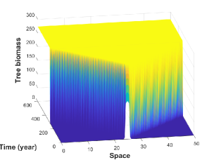
(a)

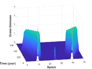
(b)

Figure 1: Illustration of the spreading of both tree (see panel (a)) and grass (see panel (b)) biomasses toward the stable forest equilibrium $\mathbf{E}_{T}=(273.3955,0)$ with system (8)-(9). $\textbf{W}=1200$ mm.yr^-1, $\tilde{\tau}=2$ yr, $d_{T}$=0.001 and $d_{G}$=0.002. Remaining parameters are in Table 1, page 1.

In the setting of the forest encroachment phenomenon, we carry out numerical simulations to compute the spreading speed of forest biomass. We investigate the relationship between the tree biomass diffusion coefficient and its spreading speed. To estimate the spreading speed of the tree biomass that undergoes a forest encroachment, grass biomass diffusion coefficient $d_{G}$ is kept constant and equal to 0.002 while tree biomass diffusion coefficient $d_{T}$ varies in the range $[0.001,0.9]$. In the diffusive logistic equation, a linear relationship is obtained between the wave speed and the square root of the diffusion coefficient (e.g. Volpert Volpert2014 , Yatat et al. Yatat2017b , Yatat and Dumont YatatDumont2018 ). Hence, for the tree biomass, we consider an equation of the form $c_{T}(d_{T})=a_{1}d_{T}^{a_{2}}$ to be fitted for the data shown in Fig. 2(b), page 2, where $c_{T}\in[0.0865,1.6899]$. We found that $a_{1}\in(1.7624,1.7861)$ and $a_{2}\in(0.4816,0.4911)$ with 95% confidence. In fact, $a_{1}=1.7743$ and $a_{2}=0.48634$, with $r^{2}=1$, indicating that 100% of the variance of the data is explained by the equation.

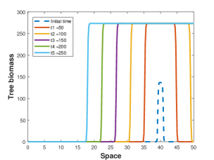
(a)

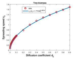
(b)

Figure 2: The forest homogeneous steady state $\mathbf{E}_{T}=(273.3955,0)$ is stable while the grassland homogeneous steady state $\mathbf{E}_{G}=(0,3.3888)$ is unstable. We illustrate the forest encroachment phenomenon (see panel (a)) with $\textbf{W}=1200$ mm.yr^-1, $\tilde{\tau}=2$ yr, $d_{T}$=0.001, $d_{G}$=0.002 and, we carry out spreading speeds fitting for tree biomass (see panel (b)). Remaining parameters are in Table 1, page 1.

With the parameter values given in Table 2, page 2, Fig. 3 illustrates the spreading of both tree and grass biomasses toward the grassland homogeneous steady state $\mathbf{E}_{G}=(0,2.1096)$. In this case, $\tilde{\mathcal{R}}_{0}=2.0425$, $\tilde{\mathcal{R}}_{1}=1.2541$ and $\tilde{\mathcal{R}}_{2}=0.9932$. Recall that $\mathbf{E}_{G}$ exists when $\tilde{\mathcal{R}}_{0}>1$ and is LAS whenever $\tilde{\mathcal{R}}_{2}<1$. We further investigate the relationship between the diffusion coefficient and the spreading speed of the grass biomass. We assume that $d_{T}=0.001$ and $d_{G}\in[0.001,1]$. Motivated by the linear relationship obtained between the wave speed and the square root of the diffusion coefficient in the diffusive logistic equation, an equation like $c_{G}(d_{G})=a_{1}d_{G}^{a_{2}}$ was fitted to the data shown in Fig. 4(b), page 4, where $c_{G}\in[0.0465,1.0877]$. We found that $a_{1}\in(1.0829,1.0935)$ and $a_{2}\in(0.4839,0.4915)$ with 95% confidence. In fact $a_{1}=1.0882$ and $a_{2}=0.48769$, with $r^{2}=1$, indicating that 100% of the variance of the data is explained by the equation.

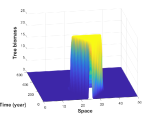
(a)

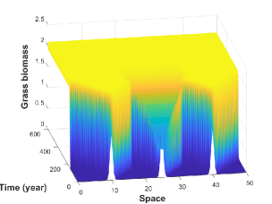
(b)

Figure 3: Illustration of the spreading of both tree (panel (a)) and grass (panel (b)) biomasses toward the grassland equilibrium $\mathbf{E}_{G}=(0,2.1096)$. $\textbf{W}=450$ mm.yr^-1, $\tilde{\tau}=2$ yr, $d_{T}$=0.001, $d_{G}$=0.002. Remaining parameters are in Table 2, page 2.

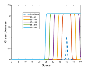
(a)

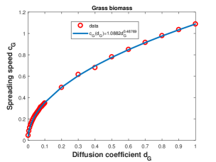
(b)

Figure 4: The forest homogeneous steady state $\mathbf{E}_{T}=(24.3905,0)$ is unstable while the grassland homogeneous steady state $\mathbf{E}_{G}=(0,2.1096)$ is stable. We illustrate the grassland encroachment phenomenon (see panel (a)) and spreading speeds fitting for grass biomass (see panel (b)). In panel (a), $\textbf{W}=450$ mm.yr^-1, $\tilde{\tau}=2$ yr, $d_{T}$=0.001, $d_{G}$=0.002. Remaining parameters are in Table 2, page 2.

5 Conclusion

In this paper, we used the vector-valued recursion equation theory (e.g. Weinberger et al. Weinberger2002 , Lewis et al. Lewis2002 , Li et al. Li2005 ) to propose a framework that deals with the existence of traveling waves for monotone systems of impulsive reaction-diffusion equations and with the computation of spreading speeds. This study extends a previous one that dealt with the impulsive Fisher-Kolmogorov-Petrowsky-Piscounov (FKPP) equation (Yatat and Dumont YatatDumont2018 ). Specifically, our results handle the aforementioned issues only in the case of monostable situations; that is, when only one of the equilibria is stable. However, the bistable case (i.e. when two equilibria are simultaneously stable) is also meaningful and needs to be studied for monotone systems of impulsive reaction-diffusion equations. Travelling waves in bistable reaction-diffusion systems without impulsive perturbations are treated in Volpert Volpert2014 (see also Yatat et al. Yatat2017 for application in the context of bistable tree-grass reaction-diffusion model).

The computation of spreading speeds and the existence of traveling waves for bistable monotone systems of impulsive reaction-diffusion equations will be the aim of future studies. It first requires to elaborate a recursion equations theory that includes bistable cases and thus extending the results of Li et al. Li2005 that only deal with monostable cases.

Appendix A Normalization procedure and model’s parameter values

We first assume that there are no fire events. In this setting, equations (8)-(9) become

$$\left\{\begin{array}[]{l}\left.\begin{array}[]{l}\displaystyle\frac{\partial T}{\partial t}=d_{T}(\textbf{W})\displaystyle\frac{\partial^{2}T}{\partial x^{2}}+\gamma_{T}(\textbf{W})\left(1-\displaystyle\frac{T}{K_{T}(\textbf{W})}\right)T-\delta_{T}T,\\ \\ \displaystyle\frac{\partial G}{\partial t}=d_{G}(\textbf{W})\displaystyle\frac{\partial^{2}G}{\partial x^{2}}+\gamma_{G}(\textbf{W})\left(1-\displaystyle\frac{G}{K_{G}(\textbf{W})}\right)G-\delta_{G}G-\eta_{TG}TG,\\ \end{array}\right.0\leq t\leq\tilde{\tau},\quad x\in\mathbb{R},\\ \end{array}\right.$$ (69)

where $\tilde{\tau}$ denotes the fire period. Following Yatat et al. [61], we have

• $\gamma_{G}(\textbf{W})=\displaystyle\frac{\gamma_{G}\times\textbf{W}}{b_{G}+\textbf{W}}$ and $\gamma_{T}(\textbf{W})=\displaystyle\frac{\gamma_{T}\times\textbf{W}}{b_{T}+\textbf{W}}$ where $\gamma_{G}$ and $\gamma_{T}$ (in yr^-1) express maximal growth of grass and tree biomasses, respectively, while half saturations $b_{G}$ and $b_{T}$ (in mm.yr^-1) determine how quickly they increase with water availability.

• $K_{T}(\textbf{W})=\displaystyle\frac{c_{T}}{1+d_{T}e^{-a_{T}\textbf{W}}}$, where $c_{T}$ (in t.ha^-1) stands for maximum value of the tree biomass carrying capacity, $a_{T}$ (mm^-1yr) controls the steepness of the curve, and $d_{T}$ controls the location of the inflection point. Similarly, $K_{G}(\textbf{W})=\displaystyle\frac{c_{G}}{1+d_{G}e^{-a_{G}\textbf{W}}}$, where $c_{G}$ (in t.ha^-1) denotes the maximum value of the grass biomass carrying capacity, $a_{G}$ (mm^-1yr) controls the steepness of the curve, and $d_{G}$ controls the location of the inflection point.

• The function $w_{G}$ is defined by

  $$w_{G}(G)=\displaystyle\frac{G^{2}}{G^{2}+\alpha_{G}^{2}},$$ (70)

  where $G$, in tons per hectare (t.ha^-1), is the grass biomass and $\alpha_{G}$ is the value taken by $G$, when the fire intensity is half of its maximum.

• the function $\psi$ is defined by

  $$\psi(T)=\lambda_{fT}^{min}+(\lambda_{fT}^{max}-\lambda_{fT}^{min})e^{-p_{T}T},$$ (71)

  where $T$, in tons per hectare (t.ha^-1), stands for the tree biomass, $\lambda_{fT}^{min}$ (in yr^-1) is the minimal loss of tree biomass due to fire in systems with a very large tree biomass, $\lambda_{fT}^{max}$ (in yr^-1) is the maximal loss of tree/shrub biomass due to fire in open vegetation (e.g. for an isolated woody individual having its crown within the flame zone), $p_{T}$ (in t^-1.ha) is proportional to the inverse of biomass suffering an intermediate level of mortality.

Assuming that requirement (7) is satisfied or, equivalently, $R_{T}=\displaystyle\frac{\gamma_{T}(\textbf{W})}{\delta_{T}}>1$ and $R_{G}=\displaystyle\frac{\gamma_{G}(\textbf{W})}{\delta_{G}}>1$. We set

$$\left\{\begin{array}[]{l}K_{T}^{\prime}=K_{T}(\textbf{W})(1-1/R_{T}),\quad K_{G}^{\prime}=K_{G}(\textbf{W})(1-1/R_{G}),\quad U=T/K_{T}^{\prime},\quad V=G/K_{G}^{\prime},\\ r=\delta_{T}(R_{T}-1)t,\quad\tau=\delta_{T}(R_{T}-1)\tilde{\tau},\quad z=x\sqrt{\delta_{T}(R_{T}-1)},\\ \lambda=\displaystyle\frac{\delta_{G}(R_{G}-1)}{\delta_{T}(R_{T}-1)},\quad\gamma=\displaystyle\frac{\eta_{TG}K_{T}^{\prime}}{\delta_{G}(R_{G}-1)}.\end{array}\right.$$ (72)

Hence, with straightforward computations, system (69) becomes

$$\left\{\begin{array}[]{l}\left.\begin{array}[]{l}\displaystyle\frac{\partial U}{\partial r}=d_{T}(\textbf{W})\displaystyle\frac{\partial^{2}U}{\partial z^{2}}+\left(1-U\right)U,\\ \\ \displaystyle\frac{\partial V}{\partial r}=d_{G}(\textbf{W})\displaystyle\frac{\partial^{2}V}{\partial z^{2}}+\lambda\left(1-V-\gamma U\right)V.\\ \end{array}\right.0\leq r\leq\tau,z\in\mathbb{R},\\ \end{array}\right.$$ (73)

Now, letting

$$\begin{array}[]{c}t:=r,\quad x:=z,\quad d_{T}:=d_{u},\quad d_{G}:=d_{v},\quad p:=p_{T}K_{T}^{\prime},\\ \quad a_{min}:=\lambda_{fT}^{min},\quad a_{max}:=\lambda_{fT}^{max},\quad\alpha=\displaystyle\frac{\alpha_{G}}{K_{G}^{\prime}}\end{array}$$ (74)

in (70), (71) and (73), we recover system (24)-(25). Furthermore, scaling (72) redefines the parameters as follows:

• The threshold $\mathcal{R}_{0}=(1-\eta)\exp(\lambda\tau)$ becomes

  $$\begin{array}[]{ccl}\tilde{\mathcal{R}}_{0}&=&(1-\eta)\exp\left(\displaystyle\frac{\gamma_{G}(\textbf{W})-\delta_{G}}{\gamma_{T}(\textbf{W})-\delta_{T}}\times(\gamma_{T}(\textbf{W})-\delta_{T})\tilde{\tau}\right),\\ &=&(1-\eta)\exp((\gamma_{G}(\textbf{W})-\delta_{G})\tilde{\tau}).\end{array}$$ (75)

• The threshold $\mathcal{R}_{1}=(1-\eta)\exp(\lambda(1-\gamma)\tau)$ becomes

  $$\begin{array}[]{ccl}\tilde{\mathcal{R}}_{1}&=&(1-\eta)\exp\left((\gamma_{G}(\textbf{W})-\delta_{G})\tilde{\tau}\left(1-\displaystyle\frac{\eta_{TG}K_{T}^{\prime}}{\gamma_{G}(\textbf{W})-\delta_{G}}\right)\right),\\ &=&(1-\eta)\exp((\gamma_{G}(\textbf{W})-\delta_{G}-\eta_{TG}K_{T}^{\prime})\tilde{\tau}).\end{array}$$ (76)

• From $\bar{v}=\displaystyle\frac{\eta}{(1-\eta)(\exp(\lambda\tau)-1)}$ one deduces that $\bar{G}=\left(1-\displaystyle\frac{\eta}{1-\eta}\times\displaystyle\frac{1}{(\exp((\gamma_{G}(\textbf{W})-\delta_{G})\tilde{\tau})-1)}\right)K_{G}^{\prime}$. Let us set $w_{\bar{G}}=\displaystyle\frac{(\bar{G})^{2}}{(\bar{G})^{2}+\alpha_{G}^{2}}$ and $w_{0}=\displaystyle\frac{(1-\bar{v})^{2}}{(1-\bar{v})^{2}+\alpha^{2}}$. Then, the threshold $\mathcal{R}_{2}=(1-a_{max}w_{0})\exp(\lambda\tau)$ becomes

  $$\begin{array}[]{ccl}\tilde{\mathcal{R}}_{2}&=&(1-\lambda_{fT}^{max}w_{\bar{G}})\exp((\gamma_{T}(\textbf{W})-\delta_{T})\tilde{\tau}).\end{array}$$ (77)

Recall that $\mathcal{R}_{0}$, $\mathcal{R}_{1}$, $\bar{v}$ and $\mathcal{R}_{2}$ are related to the normalized system (52)-(53) while $\tilde{\mathcal{R}}_{0}$, $\tilde{\mathcal{R}}_{1}$, $\bar{G}$ and $\tilde{\mathcal{R}}_{2}$ are related to the original system (8)-(9).

In Tables 1 and 2, we summarize the parameter values that are used for numerical simulations. They are chosen according to [59, 61, 62].

$c_{G}$, t.ha-1	$c_{T}$, t.ha-1	$b_{G}$, mm.yr-1	$b_{T}$, mm.yr-1	$a_{G}$, yr-1	$a_{T}$, yr-1
$20$	$450$	$501$	$1192$	$0.0029$	$0.0045$
$d_{G}$, $-$	$d_{T}$, $-$	$\gamma_{G}$, yr-1	$\gamma_{T}$, yr-1	$\delta_{G}$, yr-1	$\delta_{T}$, yr-1
$14.73$	$106.7$	$1.5$	$2$	$0.3$	$0.1$
$\eta$, $-$	$\lambda_{fT}^{min}$, $-$	$\lambda_{fT}^{max}$, $-$	$p_{T}$, t-1ha	$\alpha_{G}$, t.ha-1	$\eta_{TG}$, ha.t-1yr-1
0.7	$0.05$	$0.6$	$0.01$	2	$0.01$

Table 1: Parameter values related to system (8)-(9) at $\textbf{W}=1200$ mm.yr^-1 and $\tilde{\tau}=2$ yr. In this setting, the forest equilibrium $\mathbf{E}_{T}=(K_{T}^{\prime},0)$ is stable while the grassland equilibrium $\mathbf{E}_{G}=(0,\bar{G})$ is unstable.

$c_{G}$, t.ha-1	$c_{T}$, t.ha-1	$b_{G}$, mm.yr-1	$b_{T}$, mm.yr-1	$a_{G}$, yr-1	$a_{T}$, yr-1
$20$	$450$	$501$	$1192$	$0.0029$	$0.0045$
$d_{G}$, $-$	$d_{T}$, $-$	$\gamma_{G}$, yr-1	$\gamma_{T}$, yr-1	$\delta_{G}$, yr-1	$\delta_{T}$, yr-1
$14.73$	$106.7$	$1.5$	$2$	$0.3$	$0.1$
$\eta$, $-$	$\lambda_{fT}^{min}$, $-$	$\lambda_{fT}^{max}$, $-$	$p_{T}$, t-1ha	$\alpha_{G}$, t.ha-1	$\eta_{TG}$, ha.t-1yr-1
0.1	$0.05$	$0.6$	$0.01$	0.2	$0.01$

Table 2: Parameter values related to system (8)-(9) at $\textbf{W}=450$ mm.yr^-1 and $\tilde{\tau}=2$ yr. In this setting, the forest equilibrium $\mathbf{E}_{T}=(K_{T}^{\prime},0)$ is unstable while the grassland equilibrium $\mathbf{E}_{G}=(0,\bar{G})$ is stable.

Appendix B Another monotone increasing impulsive system

If, instead of the first coordinates change (40), one considers

$$\left\{\begin{array}[]{ccl}u_{n}&=&1-U_{n},\\ v_{n}&=&V_{n},\end{array}\right.$$ (78)

then the normalized systems (24)-(25) becomes

$$\left\{\begin{array}[]{lcl}\displaystyle\frac{\partial u_{n}}{\partial t}&=&-u_{n}(1-u_{n})+d_{u}\displaystyle\frac{\partial^{2}u_{n}}{\partial x^{2}},\quad 0\leq t\leq\tau,\quad x\in\mathbb{R},\\ \displaystyle\frac{\partial v_{n}}{\partial t}&=&\lambda v_{n}(1-v_{n})-\lambda\gamma v_{n}(1-u_{n})+d_{v}\displaystyle\frac{\partial^{2}v_{n}}{\partial x^{2}},\end{array}\right.$$ (79)

together with the updating conditions

$$\left\{\begin{array}[]{lcl}u_{n+1}(x,0)&=&w_{v}(v_{n}(x,\tau))\psi(1-u_{n}(x,\tau))(1-u_{n}(x,\tau))+u_{n}(x,\tau),\\ v_{n+1}(x,0)&=&(1-\eta)v_{n}(x,\tau).\end{array}\right.$$ (80)

As we mentioned in Subsection 4.3.3, this is a monotone increasing system and hence, reasoning as before, one can study the case where the stability of the equilibria is reversed.

References

• [1] F. Accatino and C. De Michele. Humid savanna-forest dynamics: A matrix model with vegetation-fire interactions and seasonality. Ecol. Modell., 265(0):170–179, 2013.
• [2] F. Accatino, K. Wiegand, D. Ward, and C. De Michele. Trees, grass, and fire in humid savannas: The importance of life history traits and spatial processes. Ecol. Modell., 320:135–144, 2016.
• [3] Z. Agur, L. Cojocaru, G. Mazor, R.M. Anderson, and Y.L. Danon. Pulse mass measles vaccination across age cohorts. Proc Nat Acad Sci USA, 90:11698–11702, 1993.
• [4] M.U. Akhmet, M. Beklioglu, T. Ergenc, and V.I. Tkachenko. An impulsive ratio-dependent predator–prey system with diffusion. Nonlinear Analysis: Real World Applications, 7(5):1255 – 1267, 2006.
• [5] R. Anguelov, Y. Dumont, and I.V. Yatat Djeumen. Sustainable vector/pest control using the permanent sterile insect technique. In preparation, 2019.
• [6] D. Bainov and P.S. Simeonov. Systems with impulsive effect: Stability, theory and applica-tion. John Wiley & Sons, 1989.
• [7] D.D. Bainov and P.S. Simeonov. Impulsive Differential Equations: Asymptotic properties of the solutions. World Scientfic Publishing Co., 1995.
• [8] M. Baudena, F. D’Andrea, and A. Provenzale. An idealized model for tree-grass coexistence in savannas: the role of life stage structure and fire disturbances. J. Ecol., 98:74–80, 2010.
• [9] B. Beckage, L.J. Gross, and W.J. Platt. Grass feedbacks on fire stabilize savannas. Ecol. Model., 222:2227–2233, 2011.
• [10] P.A. Bliman, D. Cardona-Salgado, Y. Dumont, and O. Vasilieva. Implementation of control strategies for sterile insect techniques. Mathematical Biosciences, 314:43 – 60, 2019.
• [11] A. Bobrowski. Functional analysis for probability and stochastic processes. Cambridge University Press, Cambridge, 2005. An introduction.
• [12] N.F. Britton. Reaction-diffusion equations and their applications to biology. Academic Press, 1986.
• [13] R.S. Cantrell and C. Cosner. Spatial Ecology via Reaction-Diffusion Equations. Wiley, 2003.
• [14] D. D’Onofrio. Stability properties of pulse vaccination strategy in seir epidemic model. Math. Biosci., 179:57–72, 2002.
• [15] C. Dufourd and Y. Dumont. Impact of environmental factors on mosquito dispersal in the prospect of sterile insect technique control. Computers & Mathematics with Applications, 66(9):1695 – 1715, 2013. BioMath 2012.
• [16] Y. Dumont and J. M. Tchuenche. mathematical studies on the sterile insect technique for the chikungunya disease and aedes albopictus. J. Math. Biol., 65 (5):809–854, 2012.
• [17] K.-J. Engel and R. Nagel. A short course on operator semigroups. Springer, 2006.
• [18] M. Fazly, M. Lewis, and H. Wang. On impulsive reaction-diffusion models in higher dimensions. SIAM J. Appl. Math., 77(1):224–246, 2017.
• [19] P.C. Fife. Mathematical Aspect of Reacting and Diffusing Systems, volume 28 of Lecture Notes in Biomathematics. Springer, Berlin, 1979.
• [20] A. Friedman. Partial Differential Equations of Parabolic Type. Englewood Cliffs, N.J. : Prentice-Hall, 1964.
• [21] J.K. Hale. Ordinary Differential Equations, second edition. Krieger Publishing Company, Malabar, Florida (USA), 1980.
• [22] J.K. Hale. Asymptotic behavior of dissipative systems. Amer. Math. Soc., Providence, 1988.
• [23] D. Henry. Geometric Theory of Semilinear Parabolic Equations. Springer-Verlag Berlin/New York, 1981.
• [24] S.I. Higgins, W.J. Bond, W. Trollope, and R.J. Williams. Physically motivated empirical models for the spread and intensity of grass fires. Int. J. Wildland Fire, 17:695–601, 2008.
• [25] Q. Huang, H. Wang, and M.A. Lewis. A hybrid continuous/discrete-time model for invasion dynamics of zebra mussels in rivers. SIAM J. Appl. Math., 77(3):854–880, 2017.
• [26] P. Klimasara and M. Tyran-Kamińska. A model for random fire induced tree-grass coexistence in savannas. Math. Appl. (Warsaw), 46(1):87–96, 2018.
• [27] A. Lakmeche and O. Arino. Bifurcation of non trivial periodic solution of impulsive differential equations arising chemotherapeutic treatment. Dyn. Cont., Disc. Imp. Sys., 7:265–287, 2000.
• [28] V. Lakshmikantham, D.D. Bainov, and P.S. Simeonov. Theory of Impulsive Differential Equations. World Scientific, Singapore, 1989.
• [29] M.A. Lewis and B. Li. Spreading speed, traveling waves, and minimal domain size in impulsive reaction–diffusion models. Bull. Math. Biol., 74(10):2383–2402, Oct 2012.
• [30] M.A. Lewis, B. Li, and F.H. Weinberger. Spreading speed and linear determinacy for two-species competition models. J. Math. Biol., 45(3):219–233, 2002.
• [31] B. Li, F.H. Weinberger, and M. Lewis. Spreading speeds as slowest wave speeds for cooperative systems. Math. Biosci., 196(1):82 – 98, 2005.
• [32] D. Li, C. Gui, and X. Luo. Impulsive vaccination seir model with nonlinear incidence rate and time delay. Math. Probl. Eng., 2013.
• [33] M. Liu, Z. Jin, and M. Haque. An impulsive predator-prey model with communicable disease in the prey species only. Nonlin. Ana. Real World App., 10:3098–3111, 2009.
• [34] Z. Liu, S. Zhong, Chun Yin, and W. Chen. On the dynamics of an impulsive reaction-diffusion predator-prey system with ratio-dependent functional response. Acta Applicandae Mathematicae, 115(3):329, Jul 2011.
• [35] J.D. Logan. An introduction to nonlinear partial differential equations, second edition. John Wiley and Sons, Inc., 2008.
• [36] J.D. Logan. Applied Partial Differential Equations. Undergraduate Texts in Mathematics. Springer International Publishing, 3 edition, 2015.
• [37] Z. Ma and J. Li. Dynamical Modeling and Analysis of Epidemics. World Scientific Publishing Co. Pte. Ltd. Singapore., 2009.
• [38] A. Okubo and S. Levin. Diffusion and ecological problems. Springer, 2001.
• [39] C. V. Pao. Nonlinear parabolic and elliptic equations. Plenum Press, New York, 1992.
• [40] B. Perthame. Parabolic Equations in Biology. Lecture Notes on Mathematical Modelling in the Life Sciences. Springer, 2015.
• [41] Y. Rogovchenko. Comparison principles for systems of impulsive parabolic equations. Annali di Matematica Pura ed Applicata, 170(1):311–328, Dec 1996.
• [42] Y. Rogovchenko. Impulsive evolution systems: Main results and new trends. Dyn. Cont. Disc. Imp. Sys., 3:57–88, 1997.
• [43] Y. Rogovchenko. Nonlinear impulsive evolution systems and applications to population models. J. Math. Anal. and Appl., 207:300–315, 1997.
• [44] H.L. Royden. Real Analysis 3rd Edition. Pearson, 1988.
• [45] N. Shigesada and K. Kawasaki. Biological invasions: theory and practice. Oxford series in ecology and evolution. Oxford University Press, 1997.
• [46] B. Shulgin, L. Stone, and Z. Agur. Pulse vaccination strategy in the sir epidemic model. Bull. Math. Bio., 60:1123–1148, 1998.
• [47] M. Strugarek, H. Bossin, and Y. Dumont. On the use of the sterile insect release technique to reduce or eliminate mosquito populations. Applied Mathematical Modelling, 68:443–470, 2019.
• [48] A.D. Synodinos, B. Tietjen, D. Lohmann, and F. Jeltsch. The impact of inter-annual rainfall variability on african savannas changes with mean rainfall. Journal of theoretical biology, 437:92–100, 2018.
• [49] A. Tchuinte Tamen, Y. Dumont, J. J. Tewa, S. Bowong, and P. Couteron. Tree-grass interaction dynamics and pulsed fires: mathematical and numerical studies. Appl. Math. Mod., 40(11-12):6165–6197, June 2016.
• [50] A. Tchuinte Tamen, Y. Dumont, J. J. Tewa, S. Bowong, and P. Couteron. A minimalistic model of tree-grass interactions using impulsive differential equations and non-linear feedback functions of grass biomass onto fire-induced tree mortality. Math. Comput. Simul, 133:265–297, March 2017.
• [51] David Terman. Comparison theorems for reaction-diffusion systems defined in an unbounded domain. Technical report, WISCONSIN UNIV-MADISON MATHEMATICS RESEARCH CENTER, 1982.
• [52] O. Vasilyeva, F. Lutscher, and M. Lewis. Analysis of spread and persistence for stream insects with winged adult stages. J. Math. Biol., 72(4):851–875, Mar 2016.
• [53] V. Volpert. Elliptic Partial Differential Equations: Volume 2. Reaction-Diffusion Equations, volume 104 of Monographs in Mathematics. Springer, 2014.
• [54] W. Walter. Differential inequalities and maximum principles: theory, new methods and applications. Nonlinear Analysis: Theory, Methods & Applications, 30(8):4695 – 4711, 1997. Proceedings of the Second World Congress of Nonlinear Analysts.
• [55] F.H. Weinberger, A.M. Lewis, and B. Li. Analysis of linear determinacy for spread in cooperative models. J. Math. Biol., 45(3):183–218, 2002.
• [56] C. Wenjun and Z. Jin. The dynamics of the constant and pulse birth in an sir epidemic model with constant recruitment. Journal of Biological Systems, 15:203–218, 2007.
• [57] S.M. White, P. Rohani, and S.M. Sait. Modelling pulsed releases for sterile insect techniques: fitness costs of sterile and transgenic males and the effects on mosquito dynamics. Journal of Applied Ecology, 47(6):1329–1339, 2010.
• [58] V. Yatat, P. Couteron, and Y. Dumont. Spatially explicit modelling of tree-grass interactions in fire-prone savannas: a partial differential equations framework. Ecol. Complexity, 36:290–313, 2018.
• [59] V. Yatat, P. Couteron, J. J. Tewa, S. Bowong, and Y. Dumont. An impulsive modelling framework of fire occurrence in a size-structured model of tree–grass interactions for savanna ecosystems. J. Math. Biol., 74(6):1425–1482, 2017.
• [60] V. Yatat and Y. Dumont. FKPP equation with impulses on unbounded domain. In R. Anguelov, M. Lachowicz (Editors), Mathematical Methods and Models in Biosciences, 2018.
• [61] V. Yatat, A. Tchuinte Tamen, Y. Dumont, and P. Couteron. A tribute to the use of minimalistic spatially-implicit models of savanna vegetation dynamics to address broad spatial scales in spite of scarce data. BIOMATH, 7:1812167, 2018.
• [62] I. V. Yatat Djeumen. Mathematical analysis of size-structured tree-grass interactions models for savanna ecosystems. PhD thesis, University of Yaoundé I, 2018.
• [63] G. Zeng, L. Chen, and L. Sun. Complexity of an sir epidemic dynamics model with impulsive vaccination control. Chaos Solit. Fract., 26:495–505, 2003.
• [64] S. Zhang, F. Wang, and L. Chen. A food chain model with impulsive perturbations and Holling IV functional response. Chaos, Solitons & Fractals, 26(3):855 – 866, 2005.
• [65] Z. Zhang, Z. Jin, and J. Pan. An SIR epidemic model with nonlinear birth pulses. Dynamics of Continuous, Discrete and Impulsive Systems. Series B: Applications and Algorithms, 14:111–128, 2008.
• [66] Z. Zhao, L. Yang, and L. Chen. Impulsive perturbations of a predator-prey system with modified Leslie-Gower and Holling type II. J. Appl. Math. Comput., 35:119–134, 2011.
• [67] S. Zheng. Nonlinear evolution equations. Chapman & Hall/CRC, 2004.