A Comparison of Adaptive and Template Matching Techniques for Radio-Isotope Identification

Abstract

We compare and contrast the effectiveness of a set of adaptive and non-adaptive algorithms for isotope identification based on gamma-ray spectra. One dimensional energy spectra are simulated for a variety of dwell-times and source to detector distances in order to reflect conditions typically encountered in radiological emergency response and environmental monitoring applications. We find that adaptive methods are more accurate and computationally efficient than non-adaptive in cases of operational interest.

1 INTRODUCTION

Algorithmic gamma-ray spectrum classification and isotope identification is a well developed field[1, 2, 3, 4, 5, 6, 7]. In radiological search and environmental health operations there are widely deployed tools based on non-adaptive template matching schemes to or supplement a human spectroscopist or even fully automate spectrum classification and isotope identification. In recent years adaptive techniques, such as neural networks and decision tress, have been developed in the research literature[1, 2]. These new techniques have not been directly compared to the historical approaches in order to gauge any increased accuracy or efficiency. Furthermore, there is a dearth of study pertaining to the often crucially important operational considerations of dwell-time for collecting each spectrum and the distance between the source and the detector. Both of these operational factors can dramatically influence the classification accuracy and, thus, yield significantly different operational outcomes. In this work, we endeavor to systematically compare two non-adaptive (template matching) techniques to more modern adaptive techniques in the context of realistic operational time and distance, and comment on the befits of each.

2 DATA

All data in this work are derived from modeled source and background templates, and have been Poisson sampled to generate sufficient training and testing sets. An advantage of using modeled data in this study is that we can precisely control, and know in advance, the true signal strength of each modeled scenario. This knowledge lends confidence and credibility to our conclusions since we will not be guessing, or relying on human spectroscopists, for the truth of each encounter. Another advantage of using modeled data is that we can avoid the class imbalance problems[2] typically associated with data sets collected from controlled laboratory or operational settings. For Example, even though ⁶⁷Cu is a much less common isotope to encounter in the environment, we will have just as many examples of it as we will the ubiquitous ^99mTc. An major disadvantage is that modeling software is known to not fully and correctly reproduce the myriad of complications that are routinely found in real-world data. Towards our goal of directly comparing and contrasting adaptive and non-adaptive methods, we asses that the advantages out-weigh the draw backs.

2.1 Templates

Spectral templates are crated using the Gamma Detector Response and Analysis Software (GADRAS)[8]. The modeled detector is a 2”$\times$4”$\times$16” NaI(Tl) crystal with 1024 channels in energy. GADRAS generates these templates using historical in-situ data collected in a laboratory setting or, as in the case of geographically specific backgrounds, in the field. The collected data are then convolved with the known detector response functions to produce an asymptotic spectral shape. This shape is asymptotic in the sense that it is modeled as a very long dwell measurement – in our case 24 hours – which is nearly free of channel-wise Poisson noise. These shapes are then scaled to the dwell-time being studied and employed both for ensemble generation and in the non-adaptive template matching techniques described below.

The templates are generated with 1024 channels, spanning the gamma-ray energy range from zero to 3 MeV. The width in energy of each channel is $\approx 2.93$ keV. The first ten bins are ignored for all of the analysis in order to approximate low-level energy discriminators often found in fielded detector systems. Thus, the gamma-ray energy spectra are divided into 1014 energy bins from 29.297 keV to 3 MeV.

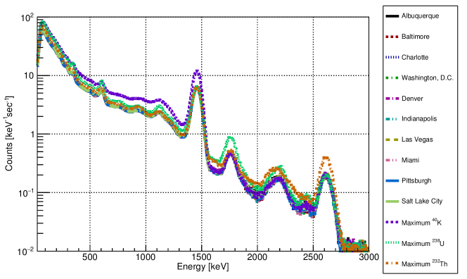
Figure 1: Modeled background spectral templates. The gamma-ray spectrum typical of 10 cities in the United States. Additionally, we generate background templates where the ratios of each of the naturally occurring radio-isotopes are maximized with respect to it’s natural range.

In Figure 1, we show the background templates typical of ten different cities in the United States. Additionally, we generate background templates where the ratios of each of the naturally occurring radio-isotopes ⁴⁰K, ²³⁸U, and ²³²Th are maximized with respect to the range over which they are commonly found in the natural environment. This variety in background templates is included in this study in an attempt to model some of the variability commonly found in operational or in situ measurements, and thus potentially increase the robustness of the methods developed and studied. We note, however, that the difference in spectral shape between the different background templates are insufficient to fully reflect operational concerns. For example, even the ⁴⁰K${}_{\text{}max}$ background is not as deviant as what might be found after a heavy rain leaches ²²²Rn from the soil[2].

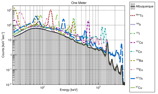
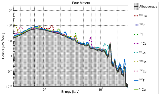
Figure 2: Modeled source spectral templates, when combined with the background typical of Albuquerque, NM. Note that both the vertical axis (Counts [keV^-1sec^-1]) and horizontal axis (Energy [keV^-1]) are logarithmically scaled in order to highlight the low-energy channels where most of the isotopic spectral peaks are present. The top panel shows the modeled detector response with one meter of separation between each source and the detector, and the bottom shows that with 4 meters of separation. The visible difference between the top and bottom panels illustrates the significant effect of atmospheric attenuation will have on observed gamma-ray energy spectra.

Nine source (i.e. signal) templates are also modeled and are listed in Table 1. The modeled isotopes were chosen to be representative of those commonly used in medical and industrial applications. The modeled activity of each isotope is roughly that often found in medicine and industry, but was further adjusted to give a (mostly) clear signal at short distances and medium dwell-times, as shown in the third column of Table 1.

The detector response was modeled with the distance between the source and detector $d\in\{1,2,4,5,6,8\}$ meters, and dwell-times $t\in\{0.25,0.5,1,2,4,8,16,32,64,128,256\}$ seconds. This range of distances and dwell-times is typical of those found in radiation health and safety applications. The source-to-detector distance induces significant decrease in signal strength due to gamma-ray attenuation in air. The last two columns of Table 1 show the effect of attenuation on the signal strength. This attenuation, and the general shape of the source templates when combined with a typical background, Albuquerque, is plotted in Figure 2 for the distances one meter and four meters.

Isotope	$N_{s}$ [sec-1]	$N_{s}/N_{b}$ [1 m]	$N_{s}/N_{b}$ [4 m]	$N_{s}/N_{b}$ [8 m]
99mTc	6756.72	1.45	0.18	0.05
192Ir	422.314	0.09	0.01	0.003
131I	5702.31	1.23	0.15	0.04
137Cs	6478.99	1.39	0.15	0.04
60Co	8636.7	1.86	0.21	0.05
133Ba	8543.61	1.84	0.20	0.05
152Eu	8151.16	1.75	0.19	0.05
207Th	7596.29	1.63	0.20	0.05
67Cu	5657.2	1.22	0.16	0.04

Table 1: The simulated isotopes considered in this study. In the second column we show the number of signal events, $N_{s}$, for a dwell-time of one second and at a distance of one meter. In the later columns we show the ratio of expected signal counts to expected background counts $N_{s}/N_{b}$ at one, four, and eight meters. This table illustrates the total number of counts associated with each modeled isotope and the diminishing signal strength at increasing distances.

2.2 Ensemble Generation

Ensembles of simulated data were generated for the purposes of both training and testing the various algorithms studied here. For each combination of 13 backgrounds, 9 isotopes, 11 dwell-time and 6 distances a simulated spectrum is generated by Poisson sampling the appropriate template. This sampling is repeated $1\times 10^{3}$ times for each of two ensembles which we label “training” and “testing” receptively. Thus each ensemble contains $7.722\times 10^{6}$ total simulated spectra. Within the two ensembles, each distance, dwell-time, and isotope combination contains $1.3\times 10^{4}$ spectral manifestations.

3 METHODS

3.1 Template Matching

Template matching techniques are ubiquitous in gamma-ray spectroscopy and have historically been used since the underlying mathematics required to implement them has been available for many decades[9, 10, 11]. These techniques are non-adaptive in the sense that they are designed to choose the model that best represents the data from a collection of predefined choices, without prior access to any data; they need not be trained.

We can express the PDF of the observed foreground spectrum as a function of gamma-ray energy, $E$, as a linear combination of the background template and the isotope (i.e. signal) template,

$$f(E|n_{b},n_{s})=n_{b}f_{b}(E)+n_{s}f_{s}(E),$$ (1)

where $n_{b}$ and $n_{s}$ are the fit parameters associated with the number of background and signal events, respectively. The functions $f_{b}(E)$ and $f_{s}(E)$ represent the background and signal templates, respectively, normalized such that they each integrate to unity over the range 29.297 keV to 3 MeV.

A binned likelihood objective function is constructed, using the standard approach[11], from the Poisson probability of observing $N_{i}$ counts in a bin,

$$\mathcal{L}(n_{b},n_{s})=\prod_{i=1}^{1014}\left(f(E_{i}|n_{b},n_{s})\right)^{N_{i}}e^{-f(E_{i}|n_{b},n_{s})}/N_{i}!,$$ (2)

where $E_{i}$ is the energy of each bin and $N_{i}$ is the observed simulated counts in each bin. For numerical effectiveness the monotonic property of the logarithm can be exploited, and non-parameter dependent terms dropped, such that the actual function to be minimized with respect to the parameters $n_{b}$ and $n_{s}$ is

$$\Lambda(n_{b},n_{s})\equiv-\ln\mathcal{L}(n_{b},n_{s})\equiv\sum_{i=1}^{1014}f(E_{i}|n_{b},n_{s})-N_{i}\ln f(E_{i}|n_{b},n_{s}).$$ (3)

If, and only if, the number of observed counts in each bin is large enough one may minimize the $\chi^{2}$ objective function,

$$\chi^{2}(n_{b},n_{s})=\sum_{i=1}^{1014}\frac{\left(N_{i}-f(E_{i}|n_{b},n_{s})\right)^{2}}{f(E_{i}|n_{b},n_{s})}.$$ (4)

For most of the cases under consideration in this work, and indeed most of the cases encountered in radiation and environmental safety, the number of counts in all bins is insufficient to justify the use of this objective function. We include it’s use in this work, however, since this objective function is commonly used in the fielded applications and as another metric against which we can compare the newer, adaptive, techniques.

Once the objective function(s) is minimized with respect to the free parameters, we choose the isotope template that best represents the data by calculating the Kolmogorov-Smirnov probability for each with respect to the simulated binned data under consideration. We further restrict the choice of best fit template by not allowing the fraction of fit signal events, $n_{s}$, to be less than 5%, since any signal that is sufficiently close to zero would be indistinguishable from background.

3.2 Adaptive Techniques

The two adaptive methods explored in this work are dense neural networks (DNN) and convolution neural networks (CNN).

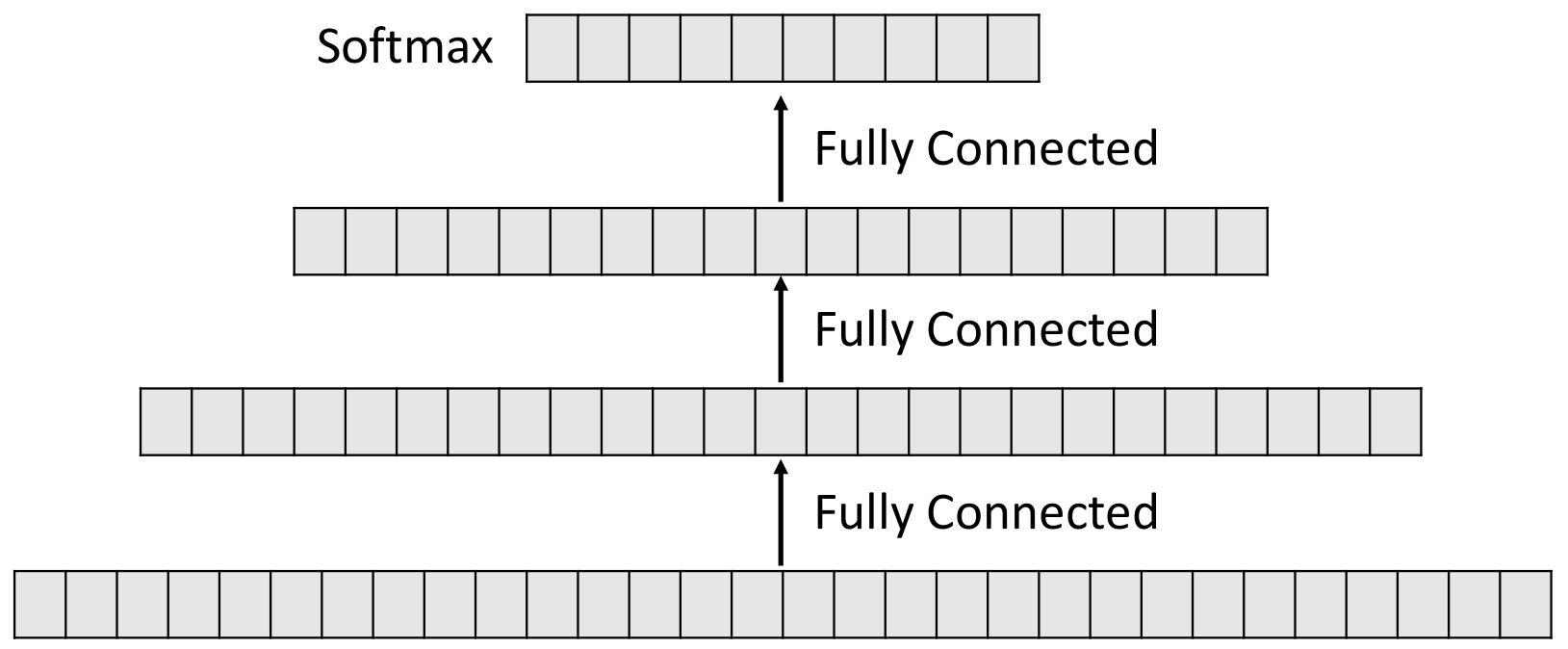
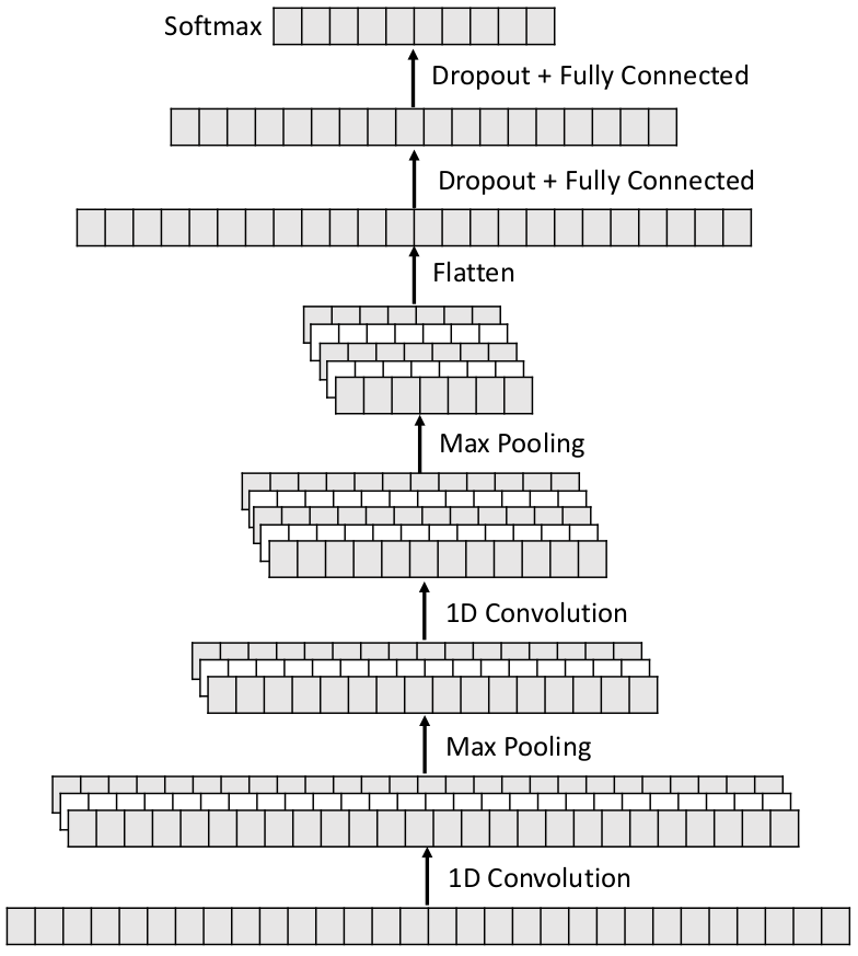
Figure 3: Left: An example representation of a dense neural network (DNN) where the input layers are the counts in each energy bin of the spectrum, the intervening layers are fully connected, and the output layer is softmax for determining the most likely isotope. In the right panel we show a deeper, more complicated convolutional neural network (CNN) where the intervening layers are successive combinations of pooling, one dimensional convolutions, flattening, and finally dropout and fully connected layers. These representations are drawn from Kamuda, et al.[1]

An example DNN architecture with two hidden layers is shown in the left panel of Figure 3. In this network, each channel of a gamma-ray spectrum is connected to each node in the next layer. These dense connections continue for each layer in the network.

An example of a CNN is shown in Figure 3. The input and output of the CNN are the same as the DNN. The difference between the CNN and DNN are the convolution and max pooling layers. Convolution layers activations are created by convolving 1-D filters with the previous layer’s signal. Max pooling is a sub-sampling operation that attempt to combine low-level features and to encourage spatial invariance by reducing the resolution of the previous layers [12]. After the convolution and pooling layers, the features are flattened into a vector and fed into a fully-connected architecture. The weights of the fully-connected network and the 1-D convolution filters are learned through training.

In general, neural networks have a tendency to memorize their training set in a process called overtraining. An overtrained neural network will tend to incorrectly identify novel data. To prevent this, regularizing hyperparameters were used in the to prevent overfitting and optimize performance. There is currently no known method to know which hyperparameters have an impact on model performance before training. Because of this, a number of hyperparameters are typically added to a model and a random hyperparameter search is used to identify those which are important [13].

Ranges of hyperparameters explored for the DNN and CNN are shown in the left and right panels of Table 2, respectively. A total of 128 networks were trained with randomly chosen hyperparameters from these ranges. The networks were trained on spectra simulated with a source-detector distance of 4 meters. The performance of each network was compared on a separate validation dataset of spectra simulated with the same source-detector distance. In each of these datasets 10 different spectra were simulated for each isotope and integration time. The hyperparameter combination that performed best on this dataset was chosen as the final training values. From these values new networks were trained using spectra simulated with source-detector distance of 4 meters.

Range Final Value Number of Layers 1 - 2 1 Number of Neurons in Each Hidden Layer 16 - 1024 128 Initial Learning Rate 10-4- 10-1 1.1 x $10^{-4}$ L2 Regularization Strength 10-2- 10-0.5 0.24 Neuron Dropout Rate 0.0 - 1.0 0.86 Batch Size 16, 32, 64, 128 64 Activation Function relu, tanh tanh Input Scaling log1p, sqrt sqrt

Hyperparameter Range Final Value Number of Filters 4, 8, 16, 32 32 Number of Convolution Layers 1, 2 1 Filter Length 2, 4, 8, 16, 32 16 Initial Learning Rate 10-4- 10-2 1.3 x 10-3 Batch Size 16, 32, 64, 128 64 Dense Layers 1 - 3 1 Nodes in each Layer 10 - 512 14 Dense Layer L2 Regularization Strength 10-3- 10-0.5 0.015 Dense Layer Neuron Dropout Rate 0 - 1 0.19 Activation Function relu, tanh tanh Input Scaling log1p, sqrt sqrt

Table 2: Left: Range of hyperparameter values for the DNN tested in a random search optimization. Right: Range of hyperparameter values for the CNN tested in a random search optimization. A total of 128 networks were trained with randomly chosen hyperparameters from these ranges, and the final values were used in for the results of this study.

4 RESULTS

There are many factors for evaluating the effectiveness of isotope classification and different end-users will give different weights to each consideration. Out perspective is primarily an operational one; we are interested in not only class-wise accuracy but also more subtle factors like computational efficiency and false-alarm rate (fall-out).

It is well understood that, once properly trained, adaptive techniques are highly computationally efficient to deploy, since they rely on simple operations such as matrix multiplication and functional computation and require no a posteriori minimization. We found this to be true here: while the temple matching techniques routinely required multiple hours to complete (even when using state of the art software[10] and running parallel-ized on 8 CPU cores), the neural networks give results in a matter of seconds.

Our primary results, in terms of isotopic class accuracy, are shown in Figures 4 and 5, which illustrate the effect of increasing dwell-time and distance. We note that in all cases the DNN performs comparably, or better, than the other methods considered. Furthermore, in the low-statistics regimes of short dwell-times and medium to long distance, the likelihood approach performs notably better than the $\chi^{2}$ objective function. Based on this evidence alone it seems reasonable to suggest that currently used software packages might consider switching to using the log-likelihood objective function.

The accuracy as a function of time for a distance of four meters for all methods, and seperated for each isotope class, is shown in Figure 6. We can see that even for long dwell-times and at this relatively close distance the non-adaptive techniques have difficulty accurately selecting ¹⁹²Ir. We note that the DNN at this distance fails at selecting background even at long dwell-times; this will be investigated further. The CNN at this distance, however, does performs notably better than the other methods.

The spectra simulated at 8 meters most drastically shows the generalization performance of each neural network. The bottome left panel of Figure 7 shows that the DNN was overfitting to the training dataset, misidentifying most isotopes as ¹⁹²Ir. Because DNN’s do not assume spatial structure (photopeaks, Compton continua) in data, this structure needs to be learned during training. If the training dataset is not diverse enough, the DNN may easily overfit to noise in a signal. This could show an inherent flaw in using an adaptive method that does not assume local structure in the data. The top left and right panels of Figure 7 show the non-adaptive methods commonly misidentifying ¹⁹²Ir, ¹³¹I, ¹³⁷Cs, and ⁶⁷Cu as background in spectra measured at 8 meters.

Because CNN’s do use the signals local spatial structure, they my be more robust when generalizing to new signals. The bottom right panel of Figure 7 shows that despite the differences between the training dataset, the CNN does generalize well to the spectra measured at 8 meters.

Finally, in Figure 8 we show the full confusion matrices for each method at a distance of 8 meters and a dwell-time of 256 seconds. We note that while all methods tend to favor mis-classifying all isotopes as background, the DNN show the most potential for extracting accurate information when the signal strength is subtle, but clearly non-zero.

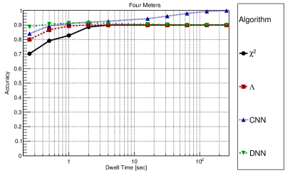
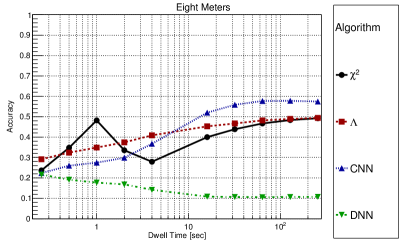
Figure 4: The accuracy of each method as a function of dwell-time at a distance of 4 meters (left) and 8 meters (right).

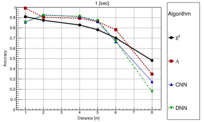
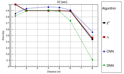
Figure 5: The accuracy of each method as a function of distance for a dwell-time 1 second (left) and 32 seconds (right).

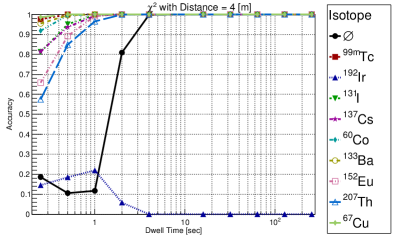
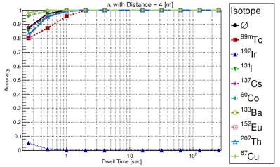
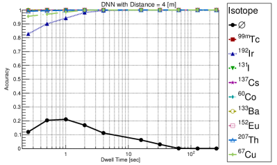
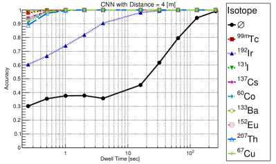
Figure 6: The class-wise accuracy of the methods as a function of dwell-time at a distance of 4 meters.

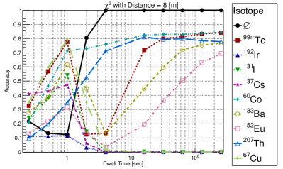
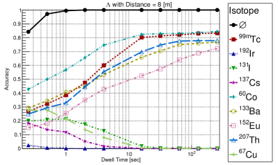
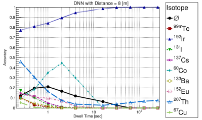
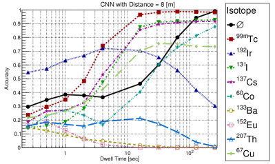
Figure 7: The class-wise accuracy of the methods as a function of dwell-time at a distance of 8 meters.

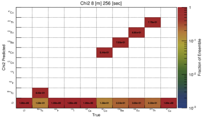
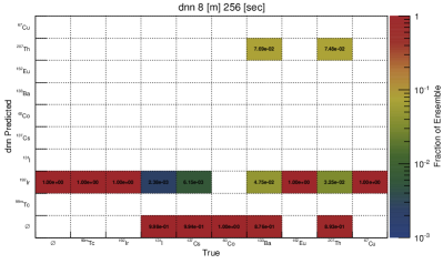
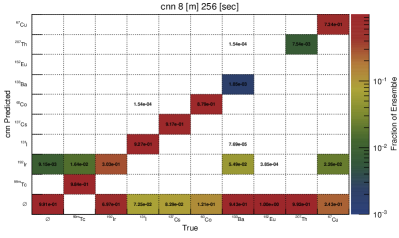
Figure 8: The confusion matrix for each method at a distance of 8 meters and dwell-time of 256 seconds.

References

- [1] Kamuda, M., Zhao, J., and Huff, K., “A comparison of machine learning methods for automated gamma-ray spectroscopy,” Nuclear Instruments and Methods in Physics Research, Section A: Accelerators, Spectrometers, Detectors and Associated Equipment (1 2018).
- [2] Sharma, S., Bellinger, C., Japkowicz, N., Berg, R., and Ungar, K., “Anomaly detection in gamma ray spectra: A machine learning perspective,” 2012 IEEE Symposium on Computational Intelligence for Security and Defence Applications (July 2012). IEEE Xplore: 31 August 2012.
- [3] Ford, W. P., Hague, E., McCullough, T., Moore, E. T., and Turk, J., “Threat determination for radiation detection from the remote sensing laboratory,” Proceedings of the SPIE 10644, 106440G (2018).
- [4] Moore, E. T. et al., “Analysis of gamma-ray spectrum using transfer learning,” https://arxiv.org/ (2019). in DRAFT.
- [5] Moore, E. T., Ford, W. P., Hague, E. J., and Turk, J. L., “Algorithm development for targeted isotopics,” (2018).
- [6] Moore, E. T., Ford, W. P., Hague, E. J., and Turk, J. L., “Algorithm development for targeted isotopics,” Site-Directed Research and Development - FY 2018 (2019).
- [7] Hague, E. J., Ford, W. P., McCullough, T., Moore, E. T., and Turk, J., “Machine learning for gamma spectra,” Symposium on Radiation Measurements and Applications Ann Arbor, Michigan (June 13, 2018).
- [8] Steve M. Horne, et al., “GADRAS-DRF 18.5 user’s manual.” Accessed: March 2019.
- [9] Rene Brun, et al., “CERN ROOT data analysis framework.” Accessed: March 2019.
- [10] Wouter Verkerke and David Kirkby, “The RooFit toolkit for data modeling.” Accessed: March 2019.
- [11] Michiel Hazewinkel, “Maximum-likelihood method.” Accessed: March 2019.
- [12] Scherer, D., Müller, A., and Behnke, S., “Evaluation of pooling operations in convolutional architectures for object recognition,” in [Artificial Neural Networks – ICANN 2010 ], Diamantaras, K., Duch, W., and Iliadis, L. S., eds., 92–101, Springer Berlin Heidelberg, Berlin, Heidelberg (2010).
- [13] Bergstra, J. and Bengio, Y., “Random search for hyper-parameter optimization,” Journal of Machine Learning Research 13, 281–305 (2012).