Fast Nonlinear Fourier Transform using Chebyshev Polynomials

Abstract

We explore the class of exponential integrators known as exponential time differencing (ETD) method in this letter to design low complexity nonlinear Fourier transform (NFT) algorithms that compute discrete approximations of the scattering coefficients in terms of the Chebyshev polynomials for real values of the spectral parameter. In particular, we discuss ETD Runge-Kutta methods which yield algorithms with complexity $O(N\log^{2}N)$ (where $N$ is the number of samples of the signal) and an order of convergence that matches the underlying one-step method.

I Introduction

This letter addresses the signal processing aspect of a nonlinear Fourier transform (NFT) based optical fiber communication system which has emerged as one of the potential ways of mitigating nonlinear signal distortions at higher signal powers [1, 2]. The idea consists in encoding information in the nonlinear Fourier spectrum of the signal which is synthesized using the inverse NFT. The information can be decoded using the direct NFT which forms the primary focus of this letter. Let us note that inverse NFT algorithm of extremely high order of convergence for computing the radiative potential have been proposed [3], which coupled with a higher order convergent direct NFT via the Darboux transformation procedure, could yield a full inverse NFT with higher order of convergence.

Recently, integrating factor (IF) based exponential integrators have been successfully exploited for the purpose of developing fast direct as well as inverse NFT algorithms [4, 5, 6, 7]. In this letter, we introduce another class exponential integrators which are known as exponential time differencing (ETD) method, a name originally used in computational electrodynamics, for the purpose of designing fast NFT algorithms. This particular class of algorithms rely on FFT based fast polynomial arithmetic in the Chebyshev basis as opposed to the monomial basis considered in the aforementioned works. While ETD schemes do not have any of the drawbacks associated with the IF schemes [8], the ETD schemes offer an additional advantage that there are no restrictions on the kind of the grid employed for sampling the potential. All ETD schemes within the Runge-Kutta as well as linear multistep methods can be sped up. In this letter, however, we have chosen the Runge-Kutta methods for our exposition.

We begin our discussion with a brief review of the scattering theory closely following the formalism presented in [4]. The NFT of any signal is defined via the Zakharov-Shabat (ZS) scattering problem (henceforth referred to as the ZS problem) which can be stated as follows: For $\zeta\in\mathbb{R}$ and $\mathbf{v}=(v_{1},v_{2})^{\intercal}$, $\mathbf{v}_{t}=\left[-i\zeta\sigma_{3}+U(t)\right]\mathbf{v}$ where $\sigma_{3}=\operatorname{diag}(1,-1)$. The potential $U(t)$ is defined by $U_{11}=U_{22}=0,\,U_{12}=q(t)$ and $U_{21}=r(t)$ with $r=\alpha q^{*}$ ($\alpha\in\{+1,-1\}$). Here, $\zeta\in\mathbb{R}$ is known as the spectral parameter and $q(t)$ is the complex-valued signal. The solution of the ZS problem consists in finding the so called scattering coefficients which are defined through special solutions known as the Jost solutions which are linearly independent solutions of the ZS problem such that they have a plane-wave like behavior at $+\infty$ or $-\infty$. The Jost solution of the second kind, denoted by $\bm{\phi}(t,\zeta)$, has the asymptotic behavior $\bm{\phi}(t;\zeta)e^{i\zeta t}\rightarrow(1,0)^{\intercal}$ as $t\rightarrow-\infty$. The asymptotic behavior $\bm{\phi}(t;\zeta)\rightarrow(a(\zeta)e^{-i\zeta t},b(\zeta)e^{i\zeta t})^{\intercal}$ as $t\rightarrow\infty$ determines the scattering coefficients $a(\zeta)$ and $b(\zeta)$ for $\zeta\in\mathbb{R}$. In this letter, we primarily focus on the continuous spectrum, also referred to as the reflection coefficient, which is defined by $\rho(\xi)={b(\xi)}/{a(\xi)}$ for $\xi\in\mathbb{R}$.

II The Numerical Scheme

The exponential time differencing Runge-Kutta (ETD–RK) methods with $s$ internal stages can be characterized much in the same way as the standard Runge-Kutta method adapted to the ZS problem: Given the step-size $h>0$, an ordered set of nodes $c_{j}\in[0,1],\,j=1,2,\ldots,s$ defining the abscissas $t_{n}\leq t_{n}+c_{1}h\leq t_{n}+c_{2}h\leq\ldots\leq t_{n}+c_{s}h\leq t_{n+1}$ and the matrix-valued weight functions $a_{ij}(-i\zeta h\sigma_{3})$, $b_{i}(-i\zeta h\sigma_{3})$, the internal stages (for $j=1,2,\ldots,s$) of the ETD–RK method together with the final update read as

$$\begin{split}&\mathbf{v}_{n,j}=e^{-ic_{j}\zeta h\sigma_{3}}\mathbf{v}_{n}+h\sum_{k=1}^{s}a_{jk}(-i\zeta h\sigma_{3}){U}_{n+c_{k}}{\mathbf{v}}_{n,k},\\ &\mathbf{v}_{n+1}=e^{-i\zeta h\sigma_{3}}\mathbf{v}_{n}+h\sum_{k=1}^{s}b_{k}(-i\zeta h\sigma_{3}){U}_{n+c_{k}}\mathbf{v}_{n,k},\end{split}$$ (1)

where we have used the convention ${U}_{n+c_{k}}=U(t_{n}+c_{k}h)$. The linear system stated above can be written as

$$\begin{pmatrix}I_{2s\times 2s}-A(\zeta;h)D_{n}&0_{2s\times 2}\\ -B(\zeta;h)^{\intercal}D_{n}&\sigma_{0}\end{pmatrix}\begin{pmatrix}{\bm{\Upsilon}}_{n}\\ {\mathbf{v}}_{n+1}\end{pmatrix}=\begin{pmatrix}E(\zeta;h){\mathbf{v}}_{n}\\ e^{-i\zeta h\sigma_{3}}{\mathbf{v}}_{n}\\ \end{pmatrix},$$ (2)

where ${D}_{n}=\operatorname{diag}\left(h{U}_{n+c_{1}},h{U}_{n+c_{1}},\ldots,h{U}_{n+c_{s}}\right)$, $A(\zeta;h)=\left(a_{ij}(-i\zeta h\sigma_{3})\right)\in\mathbb{C}^{2s\times 2s}$, and, $B(\zeta;h)$, $E(\zeta;h)\in\mathbb{C}^{2s\times 2}$ and $\bm{\Upsilon}_{n}\in\mathbb{C}^{2s}$ are defined as

$$\begin{split}&B=\begin{pmatrix}b_{1}(-i\zeta h\sigma_{3})\\ \vdots\\ b_{s}(-i\zeta h\sigma_{3})\end{pmatrix},\,\,E=\begin{pmatrix}e^{-ic_{1}\zeta h\sigma_{3}}\\ \vdots\\ e^{-ic_{s}\zeta h\sigma_{3}}\end{pmatrix},\,\,{\bm{\Upsilon}}_{n}=\begin{pmatrix}{\mathbf{v}}_{n,1}\\ \vdots\\ {\mathbf{v}}_{n,s}\end{pmatrix}.\end{split}$$ (3)

The existence of a solution of the linear system (2) depends on the determinant $\Delta_{n+1}(\zeta;h)=\det\left[I_{2s\times 2s}-A(\zeta;h)D_{n}\right]$ which can be shown to be nonzero for sufficiently small $h$. For explicit RK methods, $\Delta\equiv 1$. Introducing the transfer matrix ${M}_{n+1}(\zeta;h)$, the numerical scheme can be stated as

$$\mathbf{v}_{n+1}={e^{-i\zeta h}}[\Delta_{n+1}]^{-1}{M}_{n+1}(\zeta;h)\mathbf{v}_{n}.$$ (4)

Let us remark that collocation method [9] with Legendre–Gauss–Lobatto nodes is one of the simplest methods of constructing implicit ETD–RK methods. The weight functions in this case can be stated as follows: For $k=1,2,\ldots,s$, we have $a_{1k}=0$ and

$$\begin{split}&a_{jk}(z)=\int_{0}^{c_{j}}e^{(c_{j}-\tau)z}L_{k}(\tau)d\tau,\quad j=2,3,\ldots,s-1,\\ &b_{k}(z)=\int_{0}^{1}e^{(1-\tau)z}L_{k}(\tau)d\tau=a_{sk}(z),\\ &\text{where}\,\,L_{k}(\tau)=\prod_{n\neq k,n=1}^{s}\frac{\tau-c_{n}}{c_{k}-c_{n}}=\sum_{n=1}^{s}\frac{\lambda_{n-1}^{(k)}}{(n-1)!}\tau^{n-1}.\end{split}$$ (5)

Evidently, $a_{jk}(z)=\sum_{n=1}^{s}{c_{j}^{n}\lambda_{n-1}^{(k)}}\varphi_{n}(c_{j}z)$ where

$$(n-1)!\varphi_{n}(z)=\int_{0}^{1}e^{(1-\tau)z}{\tau^{n-1}}d\tau.$$ (6)

The $\varphi$-functions defined above are central to all ETD schemes; therefore, we discuss it in more detail in Sec. II-B. In the following, we use the convention $\varphi_{0}(z)=e^{z}$, $\varphi_{j,k}=\varphi_{j}(-ic_{k}\zeta h\sigma_{3})$ and $\varphi_{j}=\varphi_{j}(-i\zeta h\sigma_{3})$ in order to represent the ETD–RK methods using the Butcher Tableau. An example of an implicit three-stage ETD–RK method is the Lobatto IIIA method of order $4$, labelled as ETD–IRK₃₄, which is given by

$$\begin{array}[]{c|ccc}0&0&0&0\\ \frac{1}{2}&\frac{1}{2}\varphi_{3,2}-\frac{3}{4}\varphi_{2,2}+\frac{1}{2}\varphi_{1,2}&\varphi_{2,2}-\varphi_{3,2}&\frac{1}{2}\varphi_{3,2}-\frac{1}{4}\varphi_{2,2}\\ 1&4\varphi_{3}-3\varphi_{2}+\varphi_{1}&4\varphi_{2}-8\varphi_{3}&4\varphi_{3}-\varphi_{2}\\ \hline\cr&4\varphi_{3}-3\varphi_{2}+\varphi_{1}&4\varphi_{2}-8\varphi_{3}&4\varphi_{3}-\varphi_{2}\end{array}$$

Noting that $\mathbf{v}_{n+1}=\mathbf{v}_{n,3}$, the transfer matrix relation can be written as $\mathbf{v}_{n+1}=e^{-i\zeta h}\Xi_{1}^{-1}\Xi_{2}\mathbf{v}_{n}$ where

$$\left\{\begin{aligned} &\Xi_{1}=\left[\sigma_{0}-a_{33}(-i\zeta h\sigma_{3})U_{n+1}\right]\det\Gamma_{n+1/2}\\ &\quad-a_{32}(-i\zeta h\sigma_{3})U_{n+1/2}\Gamma_{n+1/2}a_{23}(-i\zeta h\sigma_{3})U_{n+1},\\ &\Xi_{2}=\left[e^{-i\zeta h\sigma_{3}}+a_{31}(-i\zeta h\sigma_{3})U_{n}\right]\det\Gamma_{n+1/2}\\ &+a_{32}(-i\zeta h\sigma_{3})U_{n+1/2}\Gamma_{n+1/2}\left[e^{-\frac{1}{2}i\zeta h\sigma_{3}}+a_{21}(-i\zeta h\sigma_{3})U_{n}\right],\end{aligned}\right.$$

with $\Gamma_{n+1/2}=\sigma_{0}+a_{22}(-i\zeta h\sigma_{3})U_{n+1/2}$. Example of an explicit four-stage ETD–RK method of order $4$ is given by [8]

$$\begin{array}[]{c|cccc}0&0&0&0&0\\ \frac{1}{2}&\frac{1}{2}\varphi_{1,2}&0&0&0\\ \frac{1}{2}&0&\frac{1}{2}\varphi_{1,2}&0&0\\ 1&\frac{1}{2}\varphi_{1,2}(\varphi_{0,2}-\sigma_{0})&0&\varphi_{1,2}&0\\ \hline\cr&4\varphi_{3}-3\varphi_{2}+\varphi_{1}&2\varphi_{2}-4\varphi_{3}&2\varphi_{2}-4\varphi_{3}&4\varphi_{3}-\varphi_{2}\end{array}$$

which we label as ETD–ERK₃₄.

II-A Fast algorithm for Chebyshev nodes

Let the computational domain be $\Omega=[T_{1},T_{2}]$ and set $2T=T_{2}-T_{1}$. Let the number of steps be $N_{s}$ and $h=2T/N_{s}$. The grid is defined by $t_{n}=T_{1}+nh/2,\,\,n=0,1,\ldots,N,$ with $t_{N}=T_{2}$ where $N=2N_{s}$ is the number of samples. Consider the Jost solution $\bm{\phi}(t;\zeta)$: $\bm{\phi}(T_{1};\zeta)=(1,0)^{\intercal}e^{-i\zeta T_{1}}$ and ${\bm{\phi}}(T_{2};\zeta)=(a(\zeta)e^{-i\zeta T_{2}},b(\zeta)e^{+i\zeta T_{2}})^{\intercal}$. Let the cumulative products be denoted by $\mathcal{M}_{1\to N_{s}}={M_{N_{s}}\times\ldots\times M_{1}}$ and $\mathcal{D}_{1\to N_{s}}={\Delta_{N_{s}}\times\ldots\times\Delta_{1}}$ so that the discrete approximation to the scattering coefficients, $a$ and $b$, can be worked out to be $a_{N}={\left(\mathcal{M}_{1\to N_{s}}\right)_{11}}/\mathcal{D}_{1\to N_{s}}$ and $b_{N}=e^{-i2\zeta T_{2}}\left(\mathcal{M}_{1\to N_{s}}\right)_{21}/\mathcal{D}_{1\to N_{s}}$.

Now, let us consider the problem of computing the samples of the continuous spectrum at the $N$ Chebyshev-Gauss-Lobatto (CGL) nodes given by $\xi_{j}=-(\pi/2h)\cos\left[{\pi j}/(N-1)\right]$ for $j=0,\ldots,N-1$. Let us first note that the matrix-valued weight functions can be computed beforehand. The naive approach to forming the cumulative products $\mathcal{M}_{1\to N_{s}}$ and $\mathcal{D}_{1\to N_{s}}$ by direct multiplication evidently yields a complexity of $\mathop{\mathcal{O}}\left(N_{s}N\right)=\mathop{\mathcal{O}}\left(N^{2}\right)$. The fast algorithm, on the other hand, is based on the idea that each of the transfer matrices $M_{n}(\zeta;h)$ and the determinants $\Delta_{n}(\zeta;h)$ can be represented using a small number of Chebyshev polynomials. The motivation behind this step is to use fast polynomial arithmetic in Chebyshev basis for computing the discrete scattering coefficients. To this end, define

$$M_{n\to n+m-1}=M_{n+m-1}\times M_{n+m-2}\times\ldots\times M_{n},$$ (7)

where $m$ is a power of $2$. The strategy is to evaluate $M_{n\to n+m-1}(\xi;h)$ on $d+1$ CGL nodes by direct multiplication of the constituting matrices followed by a discrete Chebyshev transform to obtain the Chebyshev expansion coefficients:

$$M_{n\to n+m-1}(\xi;h)=\sum_{j=0}^{d}M^{(j)}_{n\to n+m-1}\mathcal{T}_{j}\left(\frac{2}{\pi}\xi h\right),$$ (8)

for $\xi\in[-\pi/2h,\pi/2h]$ where $\mathcal{T}_{j}(\cdot)$ denotes the Chebyshev polynomial of degree $j$. Next, we also extend the strategy to the determinants $\Delta_{n}$. If the total number of matrices (or determinants) to be multiplied in the Chebyshev basis was $N_{s}$ originally, the aforementioned step reduces this number to $N_{s}/m$ at an initial cost of $9md+5m^{-1}N_{s}\nu(d+1)$ where $\nu(n)$ is the cost of discrete Chebyshev transform of size $n$.

The next step is to compute the products of the matrices (or determinants) pairwise as in [6] except we use FCT instead of FFT. Let $\nu(n)$, where $n$ is a power of $2$, be the complexity of multiplying two polynomials of degree $n-1$ in the Chebyshev basis. Let $\overline{d}=d+1$ be a power of $2$ and $\varpi(n)$ denote the complexity of multiplying $n$ matrices, then $\varpi(n)=8\nu(\overline{d}n/2)+2\varpi(n/2)$. The overall complexity now depends on how the polynomial products are carried out in the Chebyshev basis which is considered next. Let us note that the Chebyshev transform of a complex vector of size $d+1$ is equivalent to the DFT of a vector of size $2d$; therefore, the complexity of the fast Chebyshev algorithm is $\varpi_{\text{FFT}}(2d)$ [10] where $\varpi_{\text{FFT}}(n)$ denotes the complexity of FFT of size $n$.

In the following, we describe a fast algorithm for multiplying polynomials in the Chebyshev basis which proceeds by defining an equivalent multiplication problem in the monomial basis [10]: Let us consider the polynomials $p(x)$ and $q(x)$ of degree $D=N-1$ stated in the Chebyshev basis: $p(x)={\hat{p}_{0}}/{2}+\sum_{j=1}^{D}\hat{p}_{j}\mathcal{T}_{j}(x)$ and $q(x)={\hat{q}_{0}}/{2}+\sum_{j=1}^{D}\hat{q}_{j}\mathcal{T}_{j}(x)$. Let $r(x)=p(x)q(x)$ be expressed as $r(x)={\hat{r}_{0}}/{2}+\sum_{j=0}^{2D}\hat{r}_{j}\mathcal{T}_{j}(x)$. Define $\alpha(x)=\sum_{j=1}^{D}p_{j}x^{j}$, $\beta(x)=\sum_{j=1}^{D}q_{j}x^{j}$ and $\bar{\alpha}(x)=\alpha(x^{-1})x^{D}$. Also define $\gamma(x)=[p_{0}+\alpha(x)][q_{0}+\beta(x)]=\sum_{j=0}^{2D}\gamma_{j}x^{j}$ and $\delta(x)=\bar{\alpha}(x)\beta(x)=\sum_{j=0}^{2D}\delta_{j}x^{j}$, then it can be shown by direct multiplication and using the property $2\mathcal{T}_{i}(x)\mathcal{T}_{j}(x)=\mathcal{T}_{i+j}(x)+\mathcal{T}_{|i-j|}(x)$, for all $i,j\in\mathbb{Z}_{+},$ that

$$2r_{j}=\left\{\begin{aligned} &\gamma_{0}+2\delta_{D},&&j=0,\\ &\gamma_{j}+\delta_{D-j}+\delta_{D+j},&&j=1,\ldots,D-1,\\ &\gamma_{j},&&j=D,\ldots,2D.\end{aligned}\right.$$ (9)

Let us show that the algorithm discussed above can be implemented using $4$ FFTs as opposed to $6$ FFTs of size $2N$ leading to a complexity estimate of $4\varpi_{\text{FFT}}(2N)+8N$. The computation of $\gamma(x)$ is straightforward yielding a complexity of $3\varpi_{\text{FFT}}(2N)+4N$. The computation of $\delta(x)$ can be carried out by employing no more than $1$ FFT of size $2N$ as follows: Define $\mu(x)=x\delta(x)=x\bar{\alpha}(x)\beta(x)$ whose degree is $2D+1<2N$. Putting $\omega=e^{i2\pi/2N}$ and $\omega_{k}=\omega^{k}$, we have $\mu_{k}=\mu(\omega_{k})=\omega\cdot\omega^{Dk}\alpha(\omega^{-k})\beta(\omega^{k})=(-1)^{k}\alpha(\omega^{2N-k})\beta(\omega^{k})$ which can be easily computed using the quantities involved in computing $\gamma(x)$. Finally, the inverse FFT of the sequence $\mu_{k}$ followed by a shift is required in order to determine $\delta(x)$ which costs $\varpi_{\text{FFT}}(2N)+4N$ multiplications yielding an overall complexity of $4\varpi_{\text{FFT}}(2N)$ where we have retained only the leading term.

Noting that $\varpi_{\text{FFT}}(n)=\mathop{\mathcal{O}}\left(n\log_{2}n\right)$, the asymptotic complexity of computing the scattering coefficients using the polynomial multiplication algorithm described above works out to be $\varpi(N_{s})=\mathop{\mathcal{O}}\left(m^{-1}\overline{d}N_{s}\log^{2}N_{s}\right)$. The original problem of evaluating the continuous spectrum at $N$ CGL nodes now reduces to carrying out an inverse discrete Chebyshev transform.

II-B The exponential functions in ETD

In ETD–RK methods, the weights turn out to be linear combinations of the so-called $\varphi$–functions defined by (6). The first few of these functions are $\varphi_{1}=(e^{z}-1)/{z}$, $\varphi_{2}=(e^{z}-z-1)/{z^{2}}$ and $\varphi_{3}=(e^{z}-{z^{2}}/{2}-z-1)/{z^{3}}$. These functions have a removable singularity at $z=0$ and it can be easily shown that $\varphi_{k}(0)={1}/{k!}$. The higher-order $\varphi$-functions can be obtained from the recurrence relation $z\varphi_{k}(z)={\varphi_{k-1}(z)-{1}/{(k-1)!}}$ which is well-conditioned for $|z|\geq 1$. For $|z|<1$, the computation of $\varphi$-functions using the expressions above suffers from cancellation errors [11]; therefore, we resort to their Padé approximants for $|z|<\epsilon$ ($\epsilon=2^{-8}$). The $[d/d]$–Padé approximant [11] is given by $\varphi_{\ell}(z)={N_{d}^{(\ell)}(z)}/{D_{d}^{(\ell)}(z)}+\mathop{\mathcal{O}}\left(z^{2d+1}\right)$ with

$$N_{d}^{(\ell)}=\sum_{j=0}^{d}\left(\sum_{k=0}^{j}\nu_{j,k}\right)z^{j}=\sum_{j=0}^{d}\nu_{j}z^{j},\quad D_{d}^{(\ell)}=\sum_{j=0}^{d}\delta_{j}z^{j},$$ (10)

where the coefficients can be computed using the recurrence relations

$$\begin{split}\nu_{j,k+1}&=-\frac{(d-k)(\ell+j-k)}{(k+1)(2d+\ell-k)}\nu_{j,k},\quad\nu_{j,0}=\frac{1}{(\ell+j)!},\\ \delta_{j+1}&=\frac{(d-j)}{(j+1)(2d+\ell-j)}\delta_{j},\quad\delta_{0}=1.\end{split}$$ (11)

For $|z|<1$, we first scale the variable $z$ to $z2^{-K}$, where $K$ is such that $|z|2^{-K}<\epsilon$, and use the $[7/7]$–Padé approximants stated above. Once the values of $\varphi_{j}(z2^{-K})$ are available, $\varphi_{j}(z)$ can be computed by a scaling procedure given by [11]

$$\begin{split}&2^{2k}\varphi_{2k}(2z)=\varphi_{k}(z)\varphi_{k}(z)+\sum_{j=k+1}^{2k}\frac{2\varphi_{j}(z)}{(2k-j)!},\\ &2^{2k+1}\varphi_{2k+1}(2z)=\left[\varphi_{k}(z)+\frac{1}{k!}\right]\varphi_{k+1}(z)+\sum_{j=k+2}^{2k+1}\frac{2\varphi_{j}(z)}{(2k+1-j)!}.\end{split}$$

The first few of these scaling relations are as follows: $2\varphi_{1}(2z)=(e^{z}+1)\varphi_{1}(z)$, $4\varphi_{2}(2z)=\varphi_{1}(z)\varphi_{1}(z)+2\varphi_{2}(z)$ and $8\varphi_{3}(2z)=\varphi_{1}(z)\varphi_{2}(z)+2\varphi_{3}(z)+\varphi_{2}(z)$.

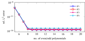
Figure 1: The figure shows the relative $\mathsf{L}^{2}$-error in approximating $\varphi_{k}$ by $\varphi_{k}(i\xi;2N)$ as a function of $N$ over $[-\pi/2,\pi/2]$.

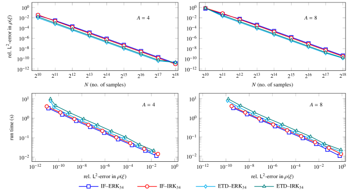
Figure 2: The convergence behavior of various NFT algorithms for the chirped secant-hyperbolic profile is plotted in the top row. The plots in the bottom row show the accuracy-complexity trade-off for each of the aforementioned algorithms.

II-C Polynomial approximation

For $z=i\xi$ with $\xi\in[-\sigma,\sigma]$, it is possible to develop polynomial approximations similar to that proposed in [12] for the $\varphi_{k}$ functions which converge exponentially. This can serve as an alternative to the rational Padé approximation method presented above. In addition, this furnishes a direct proof of the fact that the approximation (8) is exponentially accurate. Employing the expansion $\exp[i(1-\tau)\xi]=\sum_{n=0}^{\infty}(2n+1)i^{n}j_{n}(\sigma)L_{n}\left[{(1-\tau)\xi}/\sigma\right]$ where $L_{n}(\cdot)$ denotes the Legendre polynomial of degree $n$ and $j_{n}(\cdot)$ denotes the spherical Bessel function of order $n$, we have

$$\begin{split}\varphi_{k}(i\xi)&=\sum_{n=0}^{\infty}(2n+1)i^{n}j_{n}(\sigma)\int_{0}^{1}\frac{\tau^{k-1}L_{n}\left(\frac{1-\tau}{\sigma}\xi\right)}{(k-1)!}d\tau\\ &=\sum_{n=0}^{\infty}(2n+1)i^{n}j_{n}(\sigma)P_{n}\left(\frac{\xi}{\sigma};k\right),\quad k\geq 1.\end{split}$$ (12)

The first few polynomials work out to be: $P_{0}\left(x;k\right)={1}/{k!}$, $P_{1}\left(x;k\right)={x}/{(k+1)!}$ and $P_{2}\left(x;k\right)={3x^{2}}/{(k+2)!}-{1}/(2\,k!)$. For $m\geq 1$, we have the recurrence relations

$$\begin{split}&P_{2m}=2x\frac{\left(2m-\frac{1}{2}\right)}{2m+k}P_{2m-1}-\frac{(2m-k-1)}{2m+k}P_{2m-2}\\ &\qquad+\frac{(-1)^{m}\left(2m-\frac{1}{2}\right)\Gamma\left(m-\frac{1}{2}\right)}{\sqrt{\pi}(2m+k)\Gamma(m+1)\Gamma(k)},\\ &P_{2m+1}=2x\frac{\left(2m+\frac{1}{2}\right)}{2m+1+k}P_{2m}-\frac{(2m-k)}{2m+1+k}P_{2m-1},\end{split}$$ (13)

where we have suppressed the dependence on $x$ and $k$ for the sake of brevity.

Now, let $\varphi_{k}(i\xi;N)$ denote the approximation using the first $N$ terms of the expansion in (12) and $\epsilon_{N}=|\varphi_{k}(i\xi)-\varphi_{k}(i\xi;N)|$ the corresponding error. From the inequalities $|P_{n}\left(x;k\right)|\leq{1}/{k!}$ and $|(2n+1)j_{n}(\sigma)|\leq e\sqrt{{\sigma}/{2}}\left[{e\sigma}/{(2n+3)}\right]^{n}$, and, setting $\rho_{N}=(2N+3)/e\sigma>1$ (i.e. assuming $2N>e\sigma-3$), we have $\epsilon_{N}\leq\sum_{n=N}^{\infty}{|(2n+1)j_{n}(\sigma)|}/{k!}\leq C_{N}\rho_{N}^{-N}$ where $C_{N}=\sqrt{{e^{2}\sigma}/{2}}\rho_{N}/[(\rho_{N}-1)k!]$ which confirms that the rate of convergence is exponential with respect to $N$ (see Fig. 1 for a numerical example).

II-D Numerical tests

For the numerical experiments, we employ the chirped secant-hyperbolic potential given by $q(t)=A\operatorname{sech}(t)\exp[2iA\log\operatorname{sech}(t)]$ ($\alpha=-1$) considered in [7]. We set the computational domain to be $[-30,30]$ and let $A\in\{4,8\}$. Let $\Omega_{h}=[-\pi/2h,\pi/2h]$ denote the $\xi$-domain; then, the error in computing $\rho(\xi)$ is quantified by $e_{\text{rel.}}=\|\rho(\xi)-\rho_{\text{num.}}(\xi)\|_{\mathsf{L}^{2}(\Omega_{h})}/\|\rho(\xi)\|_{\mathsf{L}^{2}(\Omega_{h})}$ where $\rho_{\text{num.}}(\xi)$ is the numerical approximation and the integrals are computed using the trapezoidal rule. For the purpose of testing, we include the RK methods presented in [7] which are labelled as IF–ERK₃₄ and IF–IRK₃₄. The results are plotted in Fig. 2 which comprises convergence analysis (top row) and the trade-off between accuracy and complexity (bottom row). The results show that the ETD methods tend to be more accurate that the IF methods but their complexity-accuracy trade-off is comparable. A superior multiplication algorithm for polynomials in the Chebyshev basis may, however, dramatically change this situation.

References

• [1] M. I. Yousefi and F. R. Kschischang, “Information transmission using the nonlinear Fourier transform, Part I,” IEEE Trans. Inf. Theory, vol. 60, no. 7, pp. 4312–4369, 2014.
• [2] S. K. Turitsyn, J. E. Prilepsky, S. T. Le, S. Wahls, L. L. Frumin, M. Kamalian, and S. A. Derevyanko, “Nonlinear Fourier transform for optical data processing and transmission: advances and perspectives,” Optica, vol. 4, no. 3, pp. 307–322, Mar 2017.
• [3] V. Vaibhav, “Nonlinearly bandlimited signals,” J. Phys. A: Math. Theor., vol. 52, no. 10, p. 105202, 2019.
• [4] ——, “Fast inverse nonlinear Fourier transformation using exponential one-step methods: Darboux transformation,” Phys. Rev. E, vol. 96, p. 063302, 2017.
• [5] ——, “Fast inverse nonlinear Fourier transform,” Phys. Rev. E, vol. 98, p. 013304, 2018.
• [6] ——, “Higher order convergent fast nonlinear Fourier transform,” IEEE Photonics Technol. Lett., vol. 30, no. 8, pp. 700–703, 2018.
• [7] ——, “Efficient nonlinear Fourier transform algorithms of order four on equispaced grid,” IEEE Photonics Technol. Lett., vol. 31, no. 15, pp. 1269–1272, 2019.
• [8] S. M. Cox and P. C. Matthews, “Exponential time differencing for stiff systems,” J. Comput. Phys., vol. 176, no. 2, pp. 430–455, 2002.
• [9] M. Hochbruck and A. Ostermann, “Exponential Runge–Kutta methods for parabolic problems,” Appl. Numer. Math., vol. 53, no. 2, pp. 323–339, 2005.
• [10] P. Giorgi, “On polynomial multiplication in Chebyshev basis,” IEEE Trans. Comput., vol. 61, no. 6, pp. 780–789, 2011.
• [11] H. Berland, B. Skaflestad, and W. M. Wright, “EXPINT—A MATLAB package for exponential integrators,” ACM Trans. Math. Softw., vol. 33, no. 1, 2007.
• [12] A. Y. Suhov, “An accurate polynomial approximation of exponential integrators,” J. Sci. Comput., vol. 60, no. 3, pp. 684–698, 2014.