Backreaction on an infinite helical cosmic string

Abstract

To understand the properties of a possible cosmic string network requires knowledge of the structures on long strings, which control the breaking off of smaller loops. These structures are influenced by backreaction due to gravitational wave emission. To gain an understanding of this process, we calculate the effect of gravitational backreaction on the “helical breather”: an infinite cosmic string with a helical standing wave. We do the calculation analytically to first order in the amplitude of the oscillation. Our results for the rate of loss of length agree with the total power emitted from this system as calculated by Sakellariadou. We also find a rotation of the generators of the string that leads to an advancement of the phase of the oscillation in addition to that produced by the loss of length.

I Introduction

Symmetry breaking phase transitions in the early universe may have led to the production of topological defects, in particular cosmic strings. “Cosmic superstrings” may also have formed during the process of string-theory-based inflation. For a review of strings see Ref. Vilenkin and Shellard (2000) and of superstrings Chernoff and Tye (2015).

Cosmic strings release energy into gravitational radiation, leading to potentially observable signals Sanidas et al. (2013); Sousa and Avelino (2016); Abbott et al. (2018); Blanco-Pillado and Olum (2017); Blanco-Pillado et al. (2018a). This radiative emission reacts back on the string, decreasing its length and changing its shape. This process affects each string on small length scales and so is important in determining the detailed evolution of a string network Austin et al. (1993, 1995). Backreaction on long strings may also influence the number of loops produced and therefore the network’s gravitational emission spectra Blanco-Pillado and Olum (2017); Polchinski and Rocha (2007); Chernoff et al. (2019).

The pioneering work on cosmic string backreaction was done by Quashnock and Spergel in 1990 Quashnock and Spergel (1990). More recently, Blanco-Pillado, Olum, and Wachter have studied backreaction both analytically Wachter and Olum (2017a, b); Blanco-Pillado et al. (2018b) and numerically Blanco-Pillado et al. (2019). All such work, however, has studied oscillating loops of cosmic string. Here we begin the study of backreaction on strings that are not in the form of loops, beginning with the simple case of the “helical breather”, an infinite helical standing wave whose radius oscillates between $0$ and some value $\epsilon$. We work in the limit where $\epsilon\ll 1$, which permits an analytic calculation of the backreaction.

In Sec. II we establish the general formalism that we use to study this problem, and in Sec. III we discuss the helical breather and its symmetries. In Sec. IV we introduce a coordinate system adapted to the backreaction problem Blanco-Pillado et al. (2018b). In Sec. V we calculate the backreaction, and in Sec. VI we show how the backreaction affects the shape of the string and check the resulting loss of energy against the calculation of radiative power made by Sakellariadou Sakellariadou (1990) for this system. We conclude in Sec. VII.

II Basics

We follow the formalism of Refs. Wachter and Olum (2017b); Blanco-Pillado et al. (2018b). We work in the Nambu approximation where the cosmic string is a line-like object that traces out a two-dimensional worldsheet in spacetime. We parameterize the worldsheet by coordinates $(\tau,\sigma)$ where $\tau$ is temporal and $\sigma$ is spatial, and work in the conformal gauge where the worldsheet metric $\gamma_{ab}$ obeys $\gamma_{\tau\sigma}=0$ and $\gamma_{\sigma\sigma}=-\gamma_{\tau\tau}$. The motion of a string in a flat background, before taking account of backreaction, is described by the 4-vector

$$X(\tau,\sigma)=\frac{1}{2}\left[A(v)+B(u)\right]\,,$$ (1)

where we have defined null coordinates $u=\tau+\sigma$ and $v=\tau-\sigma$, and $A$ and $B$ are 4-vector functions depending only on $v$ and $u$ respectively, with null tangents $A^{\prime}$ and $B^{\prime}$. We can further choose the worldsheet parameter $\tau$ to be the same as the spacetime coordinate $t$, so $A^{\prime t}=B^{\prime t}=1$.

Backreaction modifies the above evolution, by introducing acceleration Quashnock and Spergel (1990)

$$X^{\gamma}_{,uv}=-\frac{1}{4}\Gamma^{\gamma}_{\alpha\beta}A^{\prime\alpha}B^{\prime\beta}\,,$$ (2)

where $\Gamma^{\gamma}_{\alpha\beta}$ is the Christoffel symbol,

$$\Gamma^{\gamma}_{\alpha\beta}=\frac{1}{2}\eta^{\gamma\delta}\left(h_{\beta\delta,\alpha}+h_{\delta\alpha,\beta}-h_{\alpha\beta,\delta}\right)\,,$$ (3)

with $h_{\alpha\beta}$ the perturbation to the flat-space metric $\eta_{\alpha\beta}$ due to the gravitational field of the string.

We can integrate the acceleration to find the changes to $A^{\prime}$ and $B^{\prime}$,

$$\Delta A^{\prime}(v) =2\int du\,X_{,uv}(u,v)\,,$$ (4a)

$$\Delta B^{\prime}(u) =2\int dv\,X_{,uv}(u,v)\,.$$ (4b)

There is some gauge (i.e., coordinate choice) freedom in the definition of $h_{\alpha\beta}$, that makes it difficult to separate physical effects on the string from artifacts. However, for a periodic source, we can perform the integrals of Eqs. (4) over $N$ periods. Effects that grow with $N$ are physical, while those that oscillate may be gauge artifacts.

The metric derivatives in Eq. (3) can be computed by Green’s function methods. The metric derivatives at some observation point are found by integrating over all source points where the string lies on the past lightcone of the observation point. We will denote quantities at the observation point with overbars and use the symbol $\delta$ to denote the difference between a quantity at the source point and the same quantity at the observation point, i.e., $\delta f=f-\bar{f}$.

III The helical breather

We will study a helical string given in Cartesian coordinates $(t,x,y,z)$ by

$$A^{\alpha} =\left(v,\epsilon\cos v,-\epsilon\sin v,-v\sqrt{1-\epsilon^{2}}\right)\,,$$ (5a)

$$B^{\alpha} =\left(u,\epsilon\cos u,\epsilon\sin u,u\sqrt{1-\epsilon^{2}}\right)\,,$$ (5b)

so that

$$X^{\alpha}=\left(t,\epsilon\cos t\cos\sigma,\epsilon\cos t\sin\sigma,\sigma\sqrt{1-\epsilon^{2}}\right)\,,$$ (6)

and the string is a helix winding around the $z$ axis with amplitude varying as $\epsilon\cos t$. See Fig. 1.

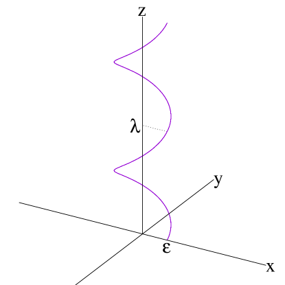
Figure 1: The helical breather at $t=0$. The string is a constant distance $\epsilon$ from the $z$ axis. The wavelength along the $z$ direction is $\lambda=2\pi\sqrt{1-\epsilon^{2}}$, while the length of string in each period is $2\pi$.

The wavelength of the helix in $z$ is $\lambda=2\pi\sqrt{1-\epsilon^{2}}$, so we will define $\lambdabar=\sqrt{1-\epsilon^{2}}$, a quantity that will occur frequently. The energy in one winding is $2\pi\mu$, where $\mu$ is the string tension, so the energy per unit $z$ is $\mu/\lambdabar$.

The maximum radius $\epsilon$ can run from $0$ to $1$. Choosing $\epsilon=0$ gives a straight string, and $\epsilon=1$ gives a circular breather loop. Here we will study the regime $\epsilon\ll 1$ and calculate the backreaction to leading order in $\epsilon$.

The string of Eq. (6) has helical symmetry: it is invariant under translation by distance $l$ in the $z$ direction combined with counterclockwise rotation by angle $2\pi l/\lambda$. Backreaction will respect this symmetry, so if we evaluate Eq. (2) at any $\sigma$ we can easily find its value at any other $\sigma$. Different times are not equivalent, however, so we will calculate the effects for any observation time $\bar{t}$ at $\bar{\sigma}=0$, and thus $\bar{u}=\bar{v}=\bar{t}$.

Symmetry considerations also restrict in what directions backreaction might act. A rotation of the system by angle $\pi$ around around the $x$ axis leaves the the string invariant (with the change of parameter $\sigma\to-\sigma$). Thus the acceleration $X^{\alpha}_{,uv}$ evaluated at $\bar{\sigma}=0$ may have only $t$ and $x$ components, which would be invariant under this rotation, not $y$ or $z$ components, which would be reversed.

In fact, helical symmetry plus energy conservation almost allows us to compute the whole evolution of the string. To preserve helical symmetry, the string must always be a helix with the same physical wavelength $\lambda$. Thus the only possibility is that the helix shrinks toward the $z$ axis while remaining helical. This new helix will have smaller energy density in each winding, and the decrease of energy density must agree with the known Sakellariadou (1990) radiation rate for this system. The only property this argument does not determine is the phase of the oscillation after backreaction. Doing the backreaction calculation allows to determine this phase, which is turns out to be nontrivial, but also this calculation may act as a starting point for similar calculations in more complex systems. So we will calculate the effects according to Eqs. (2–4) and check against Ref. Sakellariadou (1990) at the end.

IV Coordinate system

Our calculations are easier in a coordinate system adapted to the problem. Following Ref. Blanco-Pillado et al. (2018b) we define a pseudo-orthogonal coordinate system $uvcd$, as follows. Basis vectors $e_{(u)}=\bar{B^{\prime}}/2$, $e_{(v)}=\bar{A^{\prime}}/2$ are null and their inner product is $Z/4$ where

$$Z=\bar{A^{\prime}}^{\alpha}\bar{B^{\prime}}_{\alpha}=-2(1-\epsilon^{2}\sin^{2}\bar{t})\,.$$ (7)

The other two basis vectors, $e_{(c)}$ and $e_{(d)}$, are spacelike unit vectors orthogonal to $e_{(u)}$ and $e_{(v)}$ and to each other. We will use Greek letters from the middle of the alphabet for indices in $uvcd$ coordinates, and Greek letters from the beginning of the alphabet for indices in Cartesian coordinates.

In $uvcd$ coordinates, the flat metric has the form

$$\eta_{\mu\nu}=\begin{pmatrix}0&\frac{Z}{4}&0&0\\ \frac{Z}{4}&0&0&0\\ 0&0&1&0\\ 0&0&0&1\end{pmatrix}\,,$$ (8)

and Eqs. (2,3) lead to simple expressions in $uvcd$ coordinates Blanco-Pillado et al. (2018b),

$$\bar{X}^{u}_{,uv} =-\frac{2}{Z}h_{vv,u}$$ (9a)

$$\bar{X}^{v}_{,uv} =-\frac{2}{Z}h_{uu,v}$$ (9b)

$$\bar{X}^{c}_{,uv} =\frac{1}{2}\left(h_{uv,c}-h_{uc,v}-h_{vc,u}\right)$$ (9c)

$$\bar{X}^{d}_{,uv} =\frac{1}{2}\left(h_{uv,d}-h_{ud,v}-h_{vd,u}\right)\,.$$ (9d)

We will consider observation points with $\sigma=0$, which lie on the $x$ axis. Because of the symmetries of the problem, we choose $e_{(c)}$ to have only $y$ and $z$ components, while $e_{(d)}$ has only $t$ and $x$ components. This gives

$$e^{\alpha}_{(u)} =\left(\frac{1}{2},-\frac{\epsilon}{2}\sin\bar{t},\frac{\epsilon}{2}\cos\bar{t},\frac{\lambdabar}{2}\right)$$ (10a)

$$e^{\alpha}_{(v)} =\left(\frac{1}{2},-\frac{\epsilon}{2}\sin\bar{t},-\frac{\epsilon}{2}\cos\bar{t},-\frac{\lambdabar}{2}\right)$$ (10b)

$$e^{\alpha}_{(c)} =\left(0,0,-\lambdabar\gamma,\epsilon\gamma\cos\bar{t}\right)$$ (10c)

$$e^{\alpha}_{(d)} =\left(-\epsilon\gamma\sin\bar{t},\gamma,0,0\right)\,,$$ (10d)

where $\gamma=\sqrt{-2/Z}=1/\sqrt{1-\epsilon^{2}\sin^{2}\bar{t}}$. This is the Lorentz factor associated with the string velocity, $-\epsilon\sin\bar{t}$. In the particular case of $\bar{t}=0$, when the string is momentarily stationary, $e_{(d)}=e_{(x)}$ corresponds to the radial direction of the helix. At other times, $e_{(d)}$ is just a boosted version of that radial vector.

We hope there will be no confusion arising from our use of $u,v$ as labels for both the worldsheet and the spacetime coordinates. The coordinate systems are closely related: at the observation point, the motion generated by changing the worldsheet coordinate $u$ is just the spacetime vector $e_{(u)}$ and the same for $v$. The metric $h_{\mu\nu}$ is a function of spacetime position, so the notations $h_{\mu\nu,u}$ and $h_{\mu\nu,v}$ mean derivatives with respect to the $u$ and $v$ directions in spacetime. In all other cases, subscripts “$,u$” and “$,v$” mean derivatives with respect to the worldsheet variables. All components of vectors and tensors are spacetime components.

We can convert the components of a contravariant vector from $uvcd$ coordinates to Cartesian via $V^{\alpha}={M^{\alpha}}_{\mu}V^{\mu}$, where

$${M^{\alpha}}_{\mu}=\begin{pmatrix}e_{(u)}&\vrule&e_{(v)}&\vrule&e_{(c)}&\vrule&e_{(d)}\end{pmatrix}\,.$$ (11)

The transpose of this matrix will convert covariant components from Cartesian to $uvcd$, $V_{\mu}={(M^{T})_{\mu}}^{\alpha}V_{\alpha}$. In computing the metric derivatives we will often want to transform contravariant vectors to the $uvcd$ coordinates and lower the index, which we can do by $V_{\mu}={(M^{T})_{\mu}}^{\alpha}\eta_{\alpha\beta}V^{\beta}$. The components of the transformation matrix are

$${(M^{T})_{\mu}}^{\alpha}\eta_{\alpha\beta}=\begin{pmatrix}-\frac{1}{2}&-\frac{\epsilon}{2}\sin\bar{t}&\frac{\epsilon}{2}\cos\bar{t}&\frac{\lambdabar}{2}\\ -\frac{1}{2}&-\frac{\epsilon}{2}\sin\bar{t}&-\frac{\epsilon}{2}\cos\bar{t}&-\frac{\lambdabar}{2}\\ 0&0&-\lambdabar\gamma&\epsilon\gamma\cos\bar{t}\\ \epsilon\gamma\sin\bar{t}&\gamma&0&0\end{pmatrix}\,.$$ (12)

V Calculation

We can calculate the backreaction at the observation point $\bar{X}$ by integrating over all possible source points on the string world sheet that lie on the backward lightcone of $\bar{X}$. The vector pointing from $\bar{X}$ to any worldsheet point $X(u,v)$ is

$$\delta X^{\alpha}=\frac{1}{2}(\delta u+\delta v,\epsilon\left(\omega_{c}\left(\delta u,\bar{t}\right)+\omega_{c}\left(\delta v,\bar{t}\right)\right),\epsilon\left(\omega_{s}\left(\delta u,\bar{t}\right)-\omega_{s}\left(\delta v,\bar{t}\right)\right),\lambdabar\left(\delta u-\delta v\right))\,,$$ (13)

where we have defined

$$\omega_{s}(a,b) =\sin\left(a+b\right)-\sin b$$ (14a)

$$\omega_{c}(a,b) =\cos\left(a+b\right)-\cos b\,.$$ (14b)

The condition to be on the lightcone is that the interval $\mathcal{I}=\delta X^{\alpha}\delta X_{\alpha}=0$. We can write

$$\mathcal{I}=-\delta u\delta v+\frac{\epsilon^{2}}{4}\left[\left(\omega_{c}\left(\delta u,\bar{t}\right)+\omega_{c}\left(\delta v,\bar{t}\right)\right)^{2}+\left(\omega_{s}\left(\delta u,\bar{t}\right)-\omega_{s}\left(\delta v,\bar{t}\right)\right)^{2}-\left(\delta u-\delta v\right)^{2}\right]\,.$$ (15)

The intersection of the worldsheet has two branches, one that starts out in the negative $u$ direction and the other that starts out in the negative $v$ direction Blanco-Pillado et al. (2019). We will choose the former branch and add in the latter branch by symmetry. Considerations above assure us that radial and temporal contributions to the backreaction from the other branch are equal and constructive, while other spatial directions are equal and destructive.

We thus define $\delta v(\delta u)$ to be the $\delta v$ that makes $\mathcal{I}=0$ for the given $\delta u$. However, the transcendental nature of Eq. (15) makes it impossible to write $\delta v(\delta u)$ in closed form, so we must approximate. From this point forward we will take $\epsilon\ll 1$, and keep only terms that contribute at leading order in $\epsilon$. With $\epsilon=0$, $\mathcal{I}=0$ would give $\delta v=0$. Using this on the right hand side of Eq. (15), we find

$$\delta v(\delta u)=-\frac{\epsilon^{2}\delta u}{4}+\frac{\epsilon^{2}}{\delta u}\sin^{2}\frac{\delta u}{2}\,.$$ (16)

In most cases only the first term on the right hand side will contribute.

The metric derivatives can be found by integrating along our chosen branch of the backward lightcone Quashnock and Spergel (1990),

$$h_{\mu\nu,\lambda}=4G\mu\int^{0}_{-\infty}\text{d}\delta u\,\mathcal{I}_{,v}^{-1}\left[\frac{\partial}{\partial v}\left(s_{\mu\nu}\delta X_{\lambda}\mathcal{I}_{,v}^{-1}\right)\right]_{\delta v=\delta v(\delta u)}$$ (17)

where $G$ is Newton’s constant, $s_{\mu\nu}=\Sigma_{\mu\nu}\left(A^{\prime},B^{\prime}\right)$, with

$$\Sigma_{\mu\nu}\left(P,Q\right)=P_{\mu}Q_{\nu}+P_{\nu}Q_{\mu}-\eta_{\mu\nu}\left(P^{\lambda}Q_{\lambda}\right)\,,$$ (18)

and $h_{\mu\nu,\lambda}$ here denotes only the contribution from the one branch. There is a cancellation in the $uv$ term in Eq. (18) Blanco-Pillado et al. (2019),

$$\Sigma_{uv}\left(P,Q\right)=-\frac{Z}{4}(P_{c}Q_{c}+P_{d}Q_{d})\,.$$ (19)

We then calculate $\mathcal{I}_{,v}$ and the the necessary components of $s_{\mu\nu}$ and $\delta X_{\mu}$,

$$s_{uu} =\epsilon^{2}(1-\cos\delta u)$$ (20a)

$$s_{vv} =\epsilon^{2}(1-\cos\delta v)$$ (20b)

$$s_{uv} =\frac{\epsilon^{2}}{2}\left[\omega_{s}\left(\delta u,\bar{t}\right)\omega_{s}\left(\delta v,\bar{t}\right)-\omega_{c}\left(\delta u,\bar{t}\right)\omega_{c}\left(\delta v,\bar{t}\right)\right]$$ (20c)

$$s_{ud} =\left[\epsilon+\frac{\epsilon^{3}}{2}\sin^{2}\bar{t}-\epsilon^{3}\sin^{2}\frac{\delta v+2\bar{t}}{2}\right]\omega_{s}\left(\delta u,\bar{t}\right)+\epsilon^{3}\sin^{2}\frac{\delta u}{2}\omega_{s}\left(\delta v,\bar{t}\right)$$ (20d)

$$s_{vd} =\left[\epsilon+\frac{\epsilon^{3}}{2}\sin^{2}\bar{t}-\epsilon^{3}\sin^{2}\frac{\delta u+2\bar{t}}{2}\right]\omega_{s}\left(\delta v,\bar{t}\right)+\epsilon^{3}\sin^{2}\frac{\delta v}{2}\omega_{s}\left(\delta u,\bar{t}\right)$$ (20e)

$$\delta X_{u} =-\frac{\delta v}{2}+\frac{\epsilon^{2}}{4}\left[\delta v-\delta u+\left(\omega_{s}\left(\delta u,\bar{t}\right)-\omega_{s}\left(\delta v,\bar{t}\right)\right)\cos\bar{t}-\left(\omega_{c}\left(\delta u,\bar{t}\right)+\omega_{c}\left(\delta v,\bar{t}\right)\right)\sin\bar{t}\right]$$

$$=-\frac{\delta v}{2}+\frac{\epsilon^{2}}{4}\left[\delta v-\delta u+\sin\delta u-\omega_{s}(\delta v,2\bar{t})\right]$$ (21a)

$$\delta X_{v} =-\frac{\delta u}{2}+\frac{\epsilon^{2}}{4}\left[\delta u-\delta v+\left(\omega_{s}\left(\delta v,\bar{t}\right)-\omega_{s}\left(\delta u,\bar{t}\right)\right)\cos\bar{t}-\left(\omega_{c}\left(\delta u,\bar{t}\right)+\omega_{c}\left(\delta v,\bar{t}\right)\right)\sin\bar{t}\right]$$

$$=-\frac{\delta u}{2}+\frac{\epsilon^{2}}{4}\left[\delta u-\delta v+\sin\delta v-\omega_{s}(\delta u,2\bar{t})\right]$$ (21b)

$$\delta X_{d} =\frac{\epsilon}{2}\left[\left(\delta u+\delta v\right)\sin\bar{t}+\omega_{c}\left(\delta v,\bar{t}\right)+\omega_{c}\left(\delta u,\bar{t}\right)\right]$$ (21c)

$$\mathcal{I}_{,v}=-\delta u+\frac{\epsilon^{2}}{2}\left[\delta u-\delta v+\sin\delta v-\omega_{s}\left(\delta u,\delta v+2\bar{t}\right)\right]\,.$$ (22)

Here are the orders in $\epsilon$ of the above quantities and their derivatives.

$$s_{uu} \sim\epsilon^{2} s_{uu,v} =0$$ (23a)

$$s_{vv} \sim\epsilon^{2} s_{vv,v} \sim\epsilon^{2}$$ (23b)

$$s_{uv} \sim\epsilon^{2} s_{uv,v} \sim\epsilon^{2}$$ (23c)

$$s_{ud} \sim\epsilon s_{ud,v} \sim\epsilon^{3}$$ (23d)

$$s_{vd} \sim\epsilon s_{vd,v} \sim\epsilon$$ (23e)

$$\delta X_{u} \sim\delta v+\epsilon^{2} \delta X_{u,v} \sim 1+\epsilon^{2}$$ (23f)

$$\delta X_{v} \sim\delta u+\epsilon^{2} \delta X_{v,v} \sim\epsilon^{2}$$ (23g)

$$\delta X_{d} \sim\epsilon \delta X_{d,v} \sim\epsilon$$ (23h)

$$\mathcal{I}_{,v} \sim\delta u+\epsilon^{2} \mathcal{I}_{,vv} \sim\epsilon^{2}\,.$$ (23i)

We can use Eqs. (23) to see which terms we need to keep in our calculation.

Equations (20–23) apply to all $\delta u$ and $\delta v$. After we take the derivative and set $\delta v$ according to Equation (16) we can make stronger statements. First, terms in Eqs. (20–22) that are simply proportional to $\delta v$ have 2 additional powers of $\epsilon$. When $\delta v$ appears in the argument of a trigonometric function, the situation is somewhat more complicated. Consider an integral of the form

$$\int^{0}_{-\infty}\text{d}\delta u\frac{\omega(\delta v,v_{1})}{\delta u^{2}}f(\delta u)\,,$$ (24)

where $\omega$ is $\omega_{s}$ or $\omega_{c}$, $v_{1}$ is arbitrary, and $|f(\delta u)|$ is bounded by some constant. This integral is small because $\omega(\delta v,v_{1})\ll 1$ until $\delta u\sim\epsilon^{-2}$, but then the integrand is suppressed by the large denominator of order $\epsilon^{-4}$. Specifically, both $\omega_{c}$ and $\omega_{s}$ obey

$$|\omega(\delta v,v_{1})|<2$$ (25)

and also

$$|\omega(\delta v,\bar{t})|<\delta v\,,$$ (26)

since $|\text{d}\omega(\delta v,\bar{t})/\text{d}\delta v|<1$. Now we break up the integral at $-\epsilon^{-2}$. Using Eq. (25),

$$\left|\int^{-\epsilon^{-2}}_{-\infty}\text{d}\delta u\frac{\omega(\delta v,\bar{t})}{\delta u^{2}}\right|<2\epsilon^{2}\,,$$ (27)

and using Eq. (26),

$$\left|\int^{0}_{\epsilon^{-2}}\text{d}\delta u\frac{\omega(\delta v,\bar{t})}{\delta u^{2}}\right|<\left|\int^{0}_{-\epsilon^{-2}}\text{d}\delta u\frac{\delta v}{\delta u^{2}}\right|\,.$$ (28)

As $\delta u\to 0$, $\delta v\sim\delta u^{3}$, so there is no divergence near that limit. For $|\delta u|\gg 1$, $\delta v\sim\ -\epsilon^{2}\delta u/4$, giving a logarithmic divergence, so

$$\int_{0}^{\epsilon^{-2}}\text{d}\delta u\frac{\delta v}{\delta u^{2}}\sim\epsilon^{2}\ln\epsilon\,,$$ (29)

and since $f$ is bounded by a constant,

$$\int^{0}_{-\infty}\text{d}\delta u\frac{\omega(\delta v,v_{1})}{\delta u^{2}}f(\delta u)\sim\epsilon^{2}\ln\epsilon$$ (30)

at most.

This argument does not hold if $\delta u^{2}$ is replaced by $\delta u$ in the denominator of Eq. (24). For example

$$\int_{0}^{\infty}\text{d}\delta u\frac{\sin\delta v}{\delta u}=\frac{\pi}{2}+O(\epsilon^{2})\,.$$ (31)

Now we calculate the components of the backreaction using Eqs. (9, 17). We will compute only the branch that starts in the negative $\delta u$ direction and add the other by symmetry. This doubles $\bar{X}^{d}_{,uv}$, cancels $\bar{X}^{c}_{,uv}$ so that we don’t have to compute it, and adds our computed $\bar{X}^{u}_{,uv}$ and $\bar{X}^{v}_{,uv}$ to give a common backreaction in these two directions. These combinations guarantee that backreaction at $\bar{\sigma}=0$ acts only in the $t$ and $x$ directions, as discussed above.

We will find $\bar{X}^{d}_{,uv}\sim\epsilon^{3}$ and $\bar{X}^{v}_{,uv}\sim\epsilon^{4}$, so we will ignore terms of higher orders.

V.1 $h_{uv,d}$

We start by computing $\bar{X}^{d}_{,uv}$, following Eq. (9d). The first metric derivative, $h_{uv,d}$, is the simplest. First, using Equations (23c,23h,23i) we see that the term with $\mathcal{I}_{,vv}$ is negligible. Then, when we differentiate $\delta X_{d}$ we get

$$s_{uv}\delta X_{d,v}\mathcal{I}_{,v}^{-2}=\frac{\epsilon}{2}\int^{0}_{-\infty}\text{d}\delta u\frac{s_{uv}\omega_{s}(\delta v,\bar{t})}{\delta u^{2}}\,.$$ (32)

Since $|s_{uv}|<\epsilon^{2}$, this has the form of Eq. (24) with a prefactor proportional to $\epsilon^{3}$, so it does not contribute.

The remaining term depends on $s_{uv,v}=(\epsilon/2)\omega_{s}(\delta u,\delta v+2\bar{t})$ and $\delta X_{d}$ from Eq. (21c). The term involving $\delta v\sin\bar{t}$ is immediately of order $\epsilon^{5}$. The term involving $\omega_{c}(\delta v,\bar{t})$ has the form of Eq. (24) and gives $\epsilon^{5}\ln\epsilon$ at most. Ignoring these leaves us with

$$h_{uv,d}=\int^{0}_{-\infty}\text{d}\delta u\,\frac{G\mu\epsilon^{3}}{\delta u^{2}}\omega_{s}\left(\delta u,\delta v+2\bar{t}\right)\left(\omega_{c}\left(\delta u,\bar{t}\right)+\delta u\sin\bar{t}\right)\,.$$ (33)

V.2 $h_{ud,v}$

For the second metric derivative $h_{ud,v}$ we use Eqs. (23d, 23g, 23i) and see that we can differentiate any one of the factors and still have something of order $\epsilon^{3}$ in all. But closer inspection reveals that the $\delta X_{v,v}$ term goes as $\epsilon^{2}\left(1-\cos\delta v\right)$, which leads to an integral in the form of Eq. (24) that does not contribute.

For the other terms we can use $\delta X_{v}=-\delta u/2$. We then differentiate one of $s_{ud,v}$ and $\mathcal{I}_{,v}$ and expand both to leading order in $\epsilon$,

$$s_{ud,v} =\frac{\epsilon^{3}}{2}\sin\left(\delta v+2\bar{t}\right)\omega_{s}\left(\delta u,\bar{t}\right)+\epsilon^{3}\sin^{2}\frac{\delta u}{2}\cos(\delta v+\bar{t}) \mathcal{I}_{,v} =-\delta u$$ (34)

$$\mathcal{I}_{,vv} =\frac{\epsilon^{2}}{2}\left(\cos\delta v-1-\omega_{c}(\delta u,\delta v+2\bar{t})\right) s_{ud} =\epsilon\omega_{s}(\delta u,\bar{t})$$ (35)

Thus we find

$$\begin{split}h_{ud,v}=\int^{0}_{-\infty}\text{d}\delta u\,\frac{G\mu\epsilon^{3}}{\delta u^{2}}\bigg{(}&\delta u\sin\left(\delta v+2\bar{t}\right)\omega_{s}\left(\delta u,\bar{t}\right)-2\delta u\sin^{2}\frac{\delta u}{2}\cos\left(\delta v+\bar{t}\right)\\ &+\omega_{s}\left(\delta u,\bar{t}\right)\omega_{c}\left(\delta u,\delta v+2\bar{t}\right)\bigg{)}\end{split}$$ (36)

plus a term of the form of Eq. (24) that does not contribute.

V.3 $h_{vd,u}$

The final metric derivative for $\bar{X}^{d}_{,uv}$ uses Eqs (23e,23f,23i). If we don’t differentiate $\delta X_{u}$, it goes as $\epsilon^{2}$. Thus the term involving $\mathcal{I}_{,vv}$ goes as $\epsilon^{5}$. When we differentiate $s_{vd}$ we find

$$h_{vd,u}\supseteq-G\mu\epsilon\int_{-\infty}^{0}\frac{\text{d}\delta u}{\delta u^{2}}\cos(\delta v+\bar{t})\left(2\delta v+\epsilon^{2}(\delta u-\sin\delta u+\omega_{s}(\delta v,2\bar{t}))\right)\,.$$ (37)

When we differentiate $\delta X_{u}$, the leading order effect is

$$h_{vd,u}\supseteq-2G\mu\epsilon\int_{-\infty}^{0}\frac{\text{d}\delta u}{\delta u^{2}}\omega_{s}(\delta v,\bar{t})\,.$$ (38)

This is superficially $\sim\epsilon$, however the argument of Eq. (24) shows that it contributes only at order $\epsilon^{3}$. In principle there could be a contribution from expanding any of $s_{vd}$, $\delta X_{u,v}$, and $\mathcal{I}_{,v}$ to next order in $\epsilon$, but one can check that no such term contributes at order $\epsilon^{3}$.

Integrating Eq. (38) by parts gives

$$-2G\mu\epsilon\int_{-\infty}^{0}\frac{\text{d}\delta u}{\delta u}\frac{\text{d}}{\text{d}\delta u}\omega_{s}(\delta v,\bar{t})=-2G\mu\epsilon\int_{-\infty}^{0}\frac{\text{d}\delta u}{\delta u}\cos(\delta v+\bar{t})\frac{\text{d}\delta v}{\text{d}\delta u}\,.$$ (39)

From Eq. (16) we find

$$\frac{\text{d}\delta v}{\text{d}\delta u}=-\frac{\delta v}{\delta u}-\frac{\epsilon^{2}}{2}\delta u+\frac{\epsilon^{2}}{2\delta u}\sin\delta u\,.$$ (40)

When we add Eqs. (37,39), all terms cancel except the term with $\omega_{s}$, which does not contribute because it has the form of Eq. (24). Thus $h_{vd,u}=0$.

V.4 $\bar{X}^{d}_{,uv}$

To compute $\bar{X}^{d}_{,uv}$ we combine Eqs. (33,36) according to Eq. (9d). All metric derivatives above are computed only on one of the two branches. Adding the other branch multiplies the result by 2, so we just subtract Eq. (36) from Eq. (33). Many terms cancel, and we find

$$\bar{X}^{d}_{,uv}=G\mu\epsilon^{3}\int^{0}_{-\infty}\frac{\text{d}\delta u}{\delta u}\left[\cos(\delta v+\bar{t})-\cos(\delta v-\delta u+\bar{t})+\frac{2}{\delta u}\sin(\delta v+\bar{t})\left(1-\cos\delta u\right)\right]\,.$$ (41)

The overall result is

$$\bar{X}^{d}_{,uv}=G\mu\epsilon^{3}\left[\cos\bar{t}\ln\frac{\epsilon^{2}}{4}+\pi\sin\bar{t}\right]\,.$$ (42)

V.5 $h_{vv,u}$

Equation (42) will contribute a term proportional to $\epsilon^{4}$ to the time component of $\bar{X}_{,uv}$. Such a term might also arise from an $\epsilon^{4}$ in $\bar{X}^{v}_{,uv}$ and $\bar{X}^{u}_{,uv}$, so we now compute those terms at that order.

The only metric derivative appearing in $\bar{X}^{u}_{,uv}$ is $h_{vv,u}$. From Eqs (23b,23f,23i), the term where we differentiate $\mathcal{I}_{,v}$ will go as $\epsilon^{6}$ and can be ignored. The term where we differentiate $s_{vv}$ contributes

$$h_{vv,u}\supseteq-2G\mu\int^{0}_{-\infty}\text{d}\delta u\frac{\epsilon^{2}\delta v}{\delta u^{2}}\sin\delta v\,.$$ (43)

We replace the $\delta v$ that stands outside the sine function, keeping only the first term of Eq. (16), because the second term contributes at higher order in $\epsilon$ by the same analysis as Eq. (24), giving

$$h_{vv,u}\supseteq G\mu\int^{0}_{-\infty}\text{d}\delta u\frac{\epsilon^{4}}{2\delta u}\sin\delta v\,.$$ (44)

Finally, when we differentiate $\delta X_{u}$, we get a term proportional to $\epsilon^{2}$,

$$h_{vv,u}\supseteq-G\mu\int^{0}_{-\infty}\text{d}\delta u\frac{2\epsilon^{2}}{\delta u^{2}}(1-\cos\delta v)\,.$$ (45)

We should also expand $\delta X_{u,v}$ and $I_{,v}^{-2}$ to next order in $\epsilon^{2}$, but all such terms vanish because of Eq. (24).

When we combine Eqs. (44,45), the integrand is just the derivative with respect to $\delta u$ of $2\epsilon^{2}(1-\cos\delta v)/\delta u$, which vanishes at the limits of integration, plus terms in the form of Eq. (24) which are negligible. Thus the integral evaluates to zero and $\bar{X}^{u}_{,uv}=0$.

V.6 $h_{uu,v}$

For $\bar{X}^{v}_{,uv}$ we need to compute $h_{uu,v}$, following Eqs (23a,23g,23i). First notice that $s_{uu}$ doesn’t depend on $\delta v$, so when the derivative acts on it we get no contribution. The derivatives of $\mathcal{I}_{,v}$ and $\delta X_{v}$ each go as $\epsilon^{2}$, as does $s_{uu}$. So the result goes as $\epsilon^{4}$ and we can ignore subleading terms in $\mathcal{I}_{,v}$ and $\delta X_{v}$. When we differentiate $\delta X_{v}$, the result has the form of Eq. (24) and does not contribute. When we differentiate $\mathcal{I}_{,v}$ and ignore terms that do not contribute according to Eq. (24), we are left with

$$h_{uu,v}=G\mu\int^{0}_{-\infty}\text{d}\delta u\frac{\epsilon^{4}}{\delta u^{2}}(1-\cos\delta u)\omega_{c}\left(\delta u,2\bar{t}\right)=G\mu\frac{\epsilon^{4}}{2}\left(\sin 2\bar{t}\ln 4-\pi\cos 2\bar{t}\right)\,.$$ (46)

V.7 $X^{u}_{,uv}$ and $X^{v}_{,uv}$

We now compute $X^{u}_{,uv}$ and $X^{v}_{,uv}$ following Eq. (9b). Since the contribution already goes as $\epsilon^{4}$, we can ignore the factor $-2/Z=1+O(\epsilon^{2})$. Equation (46) gives the contribution from the branch that starts in the negative $\delta u$ direction. The other branch gives the same quantity in $h_{vv,u}$ and nothing in $h_{uu,v}$ so we find in all

$$\bar{X}^{v}_{,uv}=\bar{X}^{u}_{,uv}=G\mu\frac{\epsilon^{4}}{2}\left(\sin 2\bar{t}\ln 4-\pi\cos 2\bar{t}\right)\,.$$ (47)

VI Analysis

VI.1 Effect on tangent vectors

Now that we have $\bar{X}_{,uv}$, let us compute its effect on the tangent vectors $A^{\prime}$ and $B^{\prime}$. We will now drop the overbars because we are concerned only with the observation point. References Quashnock and Spergel (1990); Blanco-Pillado et al. (2019) integrated $X_{,uv}$ around the loop to find the total change to the tangent vectors. Here we don’t have a loop, but we do have a periodic system, with period $2\pi$. So we can start with the unperturbed vector,

$$A^{\prime\alpha}=(1,0,-\epsilon,-\sqrt{1-\epsilon^{2}})$$ (48)

at $v=0$ and write the change in one oscillation as

$$\Delta A^{\prime}=2\int^{4\pi}_{0}du\,X_{,uv}(u,0)\,.$$ (49)

Let us first first consider the effect of $X_{,uv}^{d}$ given by Eq. (42). This multiplies $e_{(d)}$, but we must generalize the form given in Eq. (10d) to account for the fact that we no longer have $\sigma=0$, but rather $\sigma=t=u/2$. This produces an overall rotation of the coordinate system by angle $\sigma$, so

$$e^{\alpha}_{(d)}=\left(-\epsilon\sin(u/2),\cos(u/2),\sin(u/2),0\right)\,,$$ (50)

where we have dropped factors of order $\epsilon^{2}$.

Now multiply Eq. (50) by Eq. (42). Using $\int_{0}^{4\pi}\text{d}u\sin^{2}(u/2)=\int_{0}^{4\pi}\text{d}u\cos^{2}(u/2)=2\pi$, $\int_{0}^{4\pi}\text{d}u\sin(u/2)\cos(u/2)=0$, we find

$$\Delta A^{\prime\alpha}=4\pi G\mu\epsilon^{3}\left(-\pi\epsilon,\ln\frac{\epsilon^{2}}{4},\pi,0\right)\,.$$ (51)

Equation (51) is in fact the entire backreaction, because the remaining components, $X^{u}_{,uv}$ and $X^{v}_{,uv}$ do not contribute to $\Delta A^{\prime}$. When we multiply them by $e_{(u)}$ and $e_{(v)}$ respectively, the Cartesian $y$ and $z$ components cancel, and the $x$ component is suppressed by an additional power of $\epsilon$. That leaves the time component, but it oscillates with angular frequency 2 and vanishes on integration.

The change to the time component in Eq. (51) is just the fractional change in the energy of the string in one oscillation Blanco-Pillado et al. (2019), in this case $-4\pi^{2}G\mu\epsilon^{4}$. Multiplying by the energy per unit length $\mu$ and dividing by the period gives the average rate of change of energy per unit length, $-2\pi G\mu^{2}\epsilon^{4}$, in agreement with the radiation rate computed by Sakellariadou Sakellariadou (1990) in the limit $\epsilon\ll 1$.

To find the perturbed $A^{\prime}$, we add Eq. (49) to Eq. (48) but then rescale to return the time component of $A^{\prime}$ to 1,

$$A^{\prime\alpha}_{(1)} =\left(1,4\pi G\mu\epsilon^{3}\ln\frac{\epsilon^{2}}{4},-(\epsilon-4\pi^{2}G\mu\epsilon^{3}),-\frac{\sqrt{1-\epsilon^{2}}}{1-4\pi^{2}G\mu\epsilon^{4}}\right)$$ (52)

$$=\left(1,4\pi G\mu\epsilon^{3}\ln\frac{\epsilon^{2}}{4},-\epsilon_{(1)},-\sqrt{1-{\epsilon_{(1)}}^{2}}\right)$$ (53)

with $\epsilon_{(1)}=\epsilon(1-4\pi^{2}G\mu\epsilon^{2})$. We ignored terms of order $\epsilon^{6}$ and higher. By symmetry, $B^{\prime}$ will be modified to

$$B^{\prime\alpha}_{(1)}=\left(1,4\pi G\mu\epsilon^{3}\ln\frac{\epsilon^{2}}{4},\epsilon_{(1)},\sqrt{1-{\epsilon_{(1)}}^{2}}\right)\,.$$ (54)

Thus the helix now has amplitude $\epsilon_{(1)}$, and thus the energy per unit distance in $z$ is reduced to $\mu(1+\epsilon_{(1)}^{2}/2)$, lower by $4\pi^{2}G\mu^{2}\epsilon^{4}$ than before in agreement with the above.

In addition, the new $x$ components in Eq. (52,54) represent a rotation of each vector through angle $4\pi G\mu\epsilon^{2}\ln(\epsilon^{2}/4)$. This rotation obeys the helical symmetry of the string, but it advances the time that the string comes to rest (i.e., when $A^{\prime}$ and $B^{\prime}$ point in spatially opposite directions) in successive oscillations. In the absence of any backreaction, the string would come to rest at its original position at times $2\pi N$ where $N$ is an integer. The effect of the rotation is to advance these times by

$$\Delta T_{N}^{(\text{rot})}=4\pi NG\mu\epsilon^{2}\ln(\epsilon^{2}/4)\,.$$ (55)

On the other hand, the loss of energy decreases the oscillation period so that the period after $N$ oscillations has decreased by $8\pi^{3}NG\mu\epsilon^{4}$, and thus the end of the $N$th oscillation is offset by time

$$\Delta T_{N}^{(\text{rad})}\approx-4\pi^{3}N^{2}G\mu\epsilon^{4}\,.$$ (56)

Since $\Delta T_{N}^{(\text{rad})}$ grows quadratically with $N$, it will eventually be the dominant effect controlling the times at which the helix reaches its maximum size. However, $\Delta T_{N}^{(\text{rot})}$ starts much larger, because it has two fewer powers of $\epsilon$. There is also an additional logarithmic term. Thus if one were to make a precise observation of a small-$\epsilon$ helix, the first effect one would notice is $\Delta T_{N}^{(\text{rot})}$.

VI.2 Analysis of power with backreaction treated as friction

As a simple check, we can treat the acceleration due to backreaction as arising from a force akin to frictional damping and compute the average power lost to that force. The effective force per unit length is the acceleration times the linear energy density $\mu$. It acts in the $x$ direction with magnitude $\mu X^{x}_{,tt}$.

Since $(u,v)=(\tau+\sigma,\tau-\sigma)$, $\partial/\partial u=\left(\partial/\partial\tau+\partial/\partial\sigma\right)/2$ and $\partial/\partial v=\left(\partial/\partial\tau-\partial/\partial\sigma\right)/2$, so $\partial^{2}/\partial u\partial v=\left(\partial^{2}/\partial\tau^{2}-\partial^{2}/\partial\sigma^{2}\right)/4$. Without backreaction the quantity on the right would vanish, and the effect of backreaction is to introduce an additional acceleration $X_{,tt}=4X_{,uv}$. In the $x$ direction,

$$X^{x}_{,tt}=4G\mu\epsilon^{3}\left(\cos t\ln\frac{\epsilon^{2}}{4}+\pi\sin t\right)\,,$$ (57)

and the velocity in this direction is $X^{d}_{,t}=-\epsilon\sin t$. To find the rate of change of energy per unit length we multiply the frictional force by the velocity and average over one period,

$$-\frac{2G\mu^{2}\epsilon^{4}}{\pi}\int^{2\pi}_{0}\text{d}t\,\sin t\left(\cos t\ln\frac{\epsilon^{2}}{4}+\pi\sin t\right)=-2\pi G\mu^{2}\epsilon^{4}\,.$$ (58)

again in agreement with the calculation of power radiated in Ref. Sakellariadou (1990).

VII Conclusion

We calculated the effective backreaction on the helical breather in the limit of small amplitude $\epsilon$. We found a secular decrease of length in agreement with previous work Sakellariadou (1990) for the power radiated. We also found a rotation of the $A^{\prime}$ and $B^{\prime}$ vectors, which dominates the behavior at early times. This is not associated with loss of energy to gravitational radiation, so one may say that it is a gravitational effect of the string on itself rather than the backreaction of radiation emission.

In addition to the two effects above, our calculation showed some effects that vanish when one integrates over time. It is not clear whether these should be thought of as conservative forces that take energy from the string for part of the oscillation period and return it at others, or just considered gauge artifacts. To resolve this question would require a clear definition of what one means by acceleration of the trajectory of the string as it moves in a time-varying spacetime.

In the long run we would like to understand the effect of backreaction on long strings in a cosmological network. Does backreaction smooth the string on a certain scale, so that no loops are produced below that scale? This question will have to await future work, but we hope that the present analysis of a situation simple enough to be calculated exactly (in the small-amplitude limit) will act as a starting point for further investigation.

VIII Acknowledgments

We thank J. J. Blanco-Pillado and Jeremy Wachter for helpful conversations. This work was supported in part by the National Science Foundation under Grants No. 1520792 and No. 1820902.

References

- Vilenkin and Shellard (2000) A. Vilenkin and E. P. S. Shellard, Cosmic Strings and Other Topological Defects (Cambridge University Press, 2000).
- Chernoff and Tye (2015) David F. Chernoff and S. H. Henry Tye, “Inflation, string theory and cosmic strings,” Int. J. Mod. Phys. D24, 1530010 (2015), arXiv:1412.0579 [astro-ph.CO] .
- Sanidas et al. (2013) Sotirios A. Sanidas, Richard A. Battye, and Benjamin W. Stappers, “Projected constraints on the cosmic (super)string tension with future gravitational wave detection experiments,” Astrophys. J. 764, 108 (2013), arXiv:1211.5042 [astro-ph.CO] .
- Sousa and Avelino (2016) L. Sousa and P. P. Avelino, “Probing Cosmic Superstrings with Gravitational Waves,” Phys. Rev. D94, 063529 (2016), arXiv:1606.05585 [astro-ph.CO] .
- Abbott et al. (2018) B. P. Abbott et al. (LIGO Scientific, Virgo), “Constraints on cosmic strings using data from the first Advanced LIGO observing run,” Phys. Rev. D97, 102002 (2018), arXiv:1712.01168 [gr-qc] .
- Blanco-Pillado and Olum (2017) Jose J. Blanco-Pillado and Ken D. Olum, “Stochastic gravitational wave background from smoothed cosmic string loops,” Phys. Rev. D96, 104046 (2017), arXiv:1709.02693 [astro-ph.CO] .
- Blanco-Pillado et al. (2018a) Jose J. Blanco-Pillado, Ken D. Olum, and Xavier Siemens, “New limits on cosmic strings from gravitational wave observation,” Phys. Lett. B778, 392–396 (2018a), arXiv:1709.02434 [astro-ph.CO] .
- Austin et al. (1993) Daren Austin, Edmund J. Copeland, and T. W. B. Kibble, “Evolution of cosmic string configurations,” Phys. Rev. D48, 5594–5627 (1993), arXiv:hep-ph/9307325 [hep-ph] .
- Austin et al. (1995) Daren Austin, Edmund J. Copeland, and T. W. B. Kibble, “Characteristics of cosmic string scaling configurations,” Phys. Rev. D51, 2499–2503 (1995), arXiv:hep-ph/9406379 [hep-ph] .
- Polchinski and Rocha (2007) Joseph Polchinski and Jorge V. Rocha, “Cosmic string structure at the gravitational radiation scale,” Phys. Rev. D75, 123503 (2007), arXiv:gr-qc/0702055 [GR-QC] .
- Chernoff et al. (2019) David F. Chernoff, Éanna É. Flanagan, and Barry Wardell, “Gravitational backreaction on a cosmic string: Formalism,” Phys. Rev. D99, 084036 (2019), arXiv:1808.08631 [gr-qc] .
- Quashnock and Spergel (1990) Jean M. Quashnock and David N. Spergel, “Gravitational Selfinteractions of Cosmic Strings,” Phys. Rev. D42, 2505–2520 (1990).
- Wachter and Olum (2017a) Jeremy M. Wachter and Ken D. Olum, “Gravitational smoothing of kinks on cosmic string loops,” Phys. Rev. Lett. 118, 051301 (2017a), [Erratum: Phys. Rev. Lett.121,no.14,149901(2018)], arXiv:1609.01153 [gr-qc] .
- Wachter and Olum (2017b) Jeremy M. Wachter and Ken D. Olum, “Gravitational backreaction on piecewise linear cosmic string loops,” Phys. Rev. D95, 023519 (2017b), arXiv:1609.01685 [gr-qc] .
- Blanco-Pillado et al. (2018b) Jose J. Blanco-Pillado, Ken D. Olum, and Jeremy M. Wachter, “Gravitational backreaction near cosmic string kinks and cusps,” Phys. Rev. D98, 123507 (2018b), arXiv:1808.08254 [gr-qc] .
- Blanco-Pillado et al. (2019) J. J. Blanco-Pillado, Ken D. Olum, and Jeremy M. Wachter, “Gravitational backreaction simulations of simple cosmic string loops,” (2019), arXiv:1903.06079 [gr-qc] .
- Sakellariadou (1990) M. Sakellariadou, “Gravitational waves emitted from infinite strings,” Phys. Rev. D42, 354–360 (1990), [Erratum: Phys. Rev.D43,4150(1991)].