Abstract

We present a novel numerical method aimed to characterize global behaviour, in particular chaotic diffusion, in dynamical systems. It is based on an analysis of the Poincaré recurrence statistics on massive grids of initial data or values of parameters. We concentrate on Hamiltonian systems, featuring the method separately for the cases of bounded and non-bounded phase spaces. The embodiments of the method in each of the cases are specific. We compare the performances of the proposed Poincaré recurrence method (PRM) and the custom Lyapunov exponent (LE) methods and show that they expose the global dynamics almost identically. However, a major advantage of the new method over the known global numerical tools, such as LE, FLI, MEGNO, and FA, is that it allows one to construct, in some approximation, charts of local diffusion timescales. Moreover, it is algorithmically simple and straightforward to apply.

Key words: dynamical systems, Poincaré recurrences, Lyapunov exponents, dynamical chaos, numerical methods, celestial mechanics

PACS: 02.60.-x, 05.45.-a, 05.45.Pq, 45.50.Pk, 95.10.Ce, 95.10.Fh

Introduction

A number of numerical tools, such as based on computation of Lyapunov exponents (LE), fast Lyapunov indicators (FLI), mean exponential growth number (MEGNO), and frequency analysis (FA), have been elaborated up to now to explore dynamical systems in global contexts (for a review, see, e.g., [1]). However, none of the known global tools allows one to expose diffusion rates globally. To elaborate a global numerical tool that overcomes this difficulty is just the aim of the present study. Therefore, we propose and develop a novel general method, based on a massive numerical analysis of Poincaré recurrences of orbits on fine grids of initial data or values of parameters. What makes the new method complementary to (and often advantageous over) other global numerical tools, such as LE, FLI, MEGNO, and FA, is that it allows one to characterize local diffusion rates. Indeed, LE, FLI, and MEGNO characterize local divergence of trajectories, and FA their spectral properties. Therefore, the output of the other methods does not have any universal relation to diffusion rates, whereas these are just the diffusion rates that are often needed.

The paper is organized as follows. In Section 1, we briefly review the known tools aimed to study global dynamics (LE, FLI, MEGNO, FA). In Section 2, concentrating on Hamiltonian systems, we introduce a novel global numerical method, the Poincaré recurrence method (PRM). We feature this new method separately for the cases of bounded and non-bounded phase spaces, and show that the embodiments of the method in each of the cases are specific. We compare the performances of the PRM and LE methods and show that they expose the global dynamics almost identically, but PRM is algorithmically much simpler, and it is straightforward to apply. In Section 3, we concentrate on theoretical issues of the Poincaré recurrence statistics and identify the major advantage of the new method over the custom global numerical tools: by providing the opportunity to construct charts of diffusion rates, it allows one to assess the timescales of clearing of chaotic domains of phase space in various physical and astrophysical applications. Section 4 is devoted to discussion. In Section 5, we summarize the results.

1 Numerical methods to study global
dynamics

For detecting chaos in dynamical systems, variational methods and methods of spectral analysis are mostly used. The essence of the variational methods consists in an analysis of the time evolution of trajectories with close initial conditions in phase space. In the case of chaotic dynamics, the trajectories diverge with time exponentially. A detailed analysis and a comparison of variational methods and methods of spectral analysis can be found in [2].

Numerical methods to study global behaviour of dynamical systems include, primarily, techniques based on massive computations of Lyapunov exponents [3, 4, 5, 6, 7], fast Lyapunov indicators [8], mean exponential growth number [9, 10], fundamental frequencies of motion (frequency analysis) [11, 12].

A classical method to determine the rate of divergence of close trajectories in phase space is the method based on computing the Lyapunov exponents [13, 14, 15]. A dynamical system with $N$ degrees of freedom has $2N$ Lyapunov exponents (LE), but, in practice, only the maximum LE is usually determined. By increasing the length of the time interval on which the maximum LE is calculated, for a regular orbit the value of the numerically determined finite-time maximum LE tends to zero, and for a chaotic orbit it tends to some positive non-zero value. To obtain the full Lyapunov spectrum, the HQRB-method (Householder QR-Based), in particular, can be efficiently used, developed in [16]. A comparison of various methods to compute LEs is given in [17]. Note that even very long computations may often be insufficient to distinguish between chaos and regular behaviour, and to reveal the authentic LEs, because the computed LEs, are, in fact, finite-time and local in nature; see discussion in [18].

The LE method is computationally expensive (see, e.g., a discussion in [19]). To reduce these costs, various analogues (surrogates) of the Lyapunov exponents were developed. The most popular among them are MEGNO [9, 10] and FLI [20]. The main idea of FLI, as proposed in [20], is to track the distance between two trajectories of the phase space that are initially close to each other. If at some stage of the integration the distance between the trajectories exceeds a given critical value (the threshold criterion), the dynamics is stated to be chaotic.

The MEGNO method was proposed in [9, 10]. The MEGNO parameter specifies the exponential growth factor of nearby orbits, averaged in a particular way over a finite time interval. In the case of a regular orbit, the value of the MEGNO parameter is approximately constant; for a chaotic orbit, the value of the MEGNO parameter increases with the length of the segment on which the integration is performed. MEGNO and FLI allow one to identify chaotic domains in phase space in much less (by 2–3 orders of magnitude) integration times, in comparison with the LE method. However, they do not provide any accurate estimates of the genuine Lyapunov exponents; only local approximate estimates can be obtained.

It should be noted that various simplifications and assumptions in the LE surrogates may often lead to erroneous assessments of the type of a trajectory. In particular, a disadvantage of the FLI method consists in an ambiguity in the choice of the threshold criterion for the identification of chaotic trajectories. Using MEGNO may as well lead to ambiguous conclusions; as shown in [2], in the case of a divided phase space, MEGNO may characterize the regular component ambiguously. A software package description for calculating various indicators of chaos (including LE, FLI, and MEGNO) can be found in [21].

A major spectral method is the method of frequency analysis (FA). Its description and theoretical justification are given in [22, 23, 24]. For regular orbits, the fundamental frequencies are constant, while for chaotic orbits they are not constantly defined, actions and angles varying randomly. Performing the FA at separate time intervals, one can numerically determine the current fundamental frequencies and find out whether they vary when going from one time interval to another, i.e., determine the character of the dynamics. Examples of implementation of the FA technique, as proposed in [22, 23] in the form of a numerical analysis of fundamental frequencies, can be found in [25, 26].

In addition to the general opportunity of identification of regular and chaotic domains in phase space, FA allows one to identify locations of resonances. However, FA is laborious; it may require up to $\sim 30$% of the computing time more than that required by the LE method in one and the same problem [2].

In celestial mechanics, to identify chaos in orbital or rotational motion of celestial bodies, a number of specific methods were proposed: the maximum eccentricity method (MEM) [27, 28]; methods based on massive numerical assessments of the escape/encounter conditions [29, 30]; the reversibility error method (REM) [31]. However, they are not mathematically justified in any rigorous way. Moreover, the criteria used in them for separating trajectories into chaotic and regular ones are only approximate, similar to the case of FLI.

2 The Poincaré recurrence method

In this Section, we elaborate a general method, the Poincaré recurrence method (PRM), to study global dynamics. The method is based on a massive numerical analysis of Poincaré recurrences of orbits on fine grids of initial data (or values of parameters).

2.1 Basics of the PRM

The notion of the Poincaré recurrence is of great methodological value due to the existence of the famous Poincaré recurrence theorem [32], valid in a broad class of dynamical systems, including Hamiltonian systems on which we concentrate here. Generally, the theorem states that for a volume-conserving continuous one-to-one mapping $g$, transforming a bounded domain $D$ of Euclidian space in itself ($gD=D$), in any neighbourhood $U$ of any point of $D$ there exists a point $x$ that returns to $U$: $g^{n}x\in U$ at some $n$ (see [33]). In other words, any dynamical system of certain type (in particular, with bounded phase space) recurs eventually, though it may take much time, to any neighbourhood of its initial state.

Although the theorem is valid for systems with bounded phase space, the notion of Poincaré recurrence is defined for any dynamical system. In particular, the PR method developed in this article can be used, with minimal modifications, in systems with non-bounded phase space, as demonstrated further on in Subsection 2.4.

In various statistical applications, the so-called recurrence plot technique and the recurrence quantification analysis, mostly dealing with various data series, became more and more popular in the last decades [34, 35]. The recurrence plot is defined as a set of pairs of time instants when a dynamical system returns to the same position in phase space. The recurrence plot technique has been already used in celestial mechanics: in [36], the stability of selected exoplanetary systems was globally characterized by the Rényi entropy, which was calculated by using the recurrence plot technique. Computations of first recurrence times were performed to construct a bifurcation diagram for the standard map in [37, figure 5].

And generally, computations of Poincaré recurrences have been already broadly used in assessments of properties of dynamical chaos in Hamiltonian systems. Various aspects of statistics of Poincaré recurrences were numerically and analytically explored in [38, 39, 40, 41, 42, 43].

The PRM, as proposed in this article, is intended for construction of stability charts. A stability chart, in the sense used here, is any global representation of the behaviour of any parameters, characterizing instabilities (such parameters as LE, FLI, MEGNO, or local diffusion rates) of a dynamical system, on a two-dimensional plane of initial conditions or parameters of the system. To produce a stability chart by means of PRM, the Poincaré recurrences are computed on a uniform grid in the plane of initial conditions of two selected variables (with all other initial conditions and the system parameters fixed), or on a uniform grid in the plane of two selected parameters (with all other parameters and the initial conditions fixed). The grid is defined in such a way that both regular and chaotic types of trajectories can be analyzed on the subject of the properties of their Poincaré recurrences in a representative way.

The Poincaré recurrences are calculated as follows. At each node of the defined grid, a neighbourhood of the initial point of motion of size $\varepsilon$ (either a sphere of radius $\varepsilon$ or a box with size $\varepsilon$) is defined in the phase space. By integrating numerically equations of motion, a time instant $T_{\mathrm{r}}$ is fixed when the trajectory returns to the given neighbourhood of the initial point. The integration is over when either the first Poincaré recurrence occurs or the end of the specified integration time interval is over (thus, no Poincaré recurrence time is fixed). Then, the durations of the recurrences are represented graphically on the grid; say, in a colour grade.

Note that, in the current code, we define the recurrence box either as a direct product of small linear intervals or as a small sphere. Of course, other possibilities exist. However, as one may expect (and this has been readily confirmed by our test numerical experiments), this is not the shape of the recurrence box that is important for the final clarity of a stability diagram, but its size first of all.

Grids with various numbers of nodes can be used. A key point is the choice of $\varepsilon$ at a given computation time; this issue is discussed further on in Section 4.

To obtain a non-noisy stability chart, one should normally choose the size of the recurrence box to be much smaller (by orders of magnitude) than the length of the trajectory in one recurrence. Therefore, any non-zero box-size corrections to the computed length of a recurrence are ignored in the current version of the codes. The middle point of the trajectory interval inside the recurrence box [44, Figure 1] might be a better recurrence landmark otherwise.

In the following Subsections, PRM is featured separately for the cases of bounded and non-bounded phase spaces, because the embodiments of the PRM in each of the cases are specific. To assess the performance of the PRM, we simultaneously use the traditional LE method, and compare the results.

2.2 The Poincaré recurrence method: the case of
bounded phase space

In the case of bounded phase space, the Poincaré recurrences are counted with respect to a neighbourhood of a starting point in the phase space. We take the Hénon–Heiles system [45] as a paradigm for demonstrating the opportunities of PRM in this case. It is in this problem that for the first time a chaotic behavior was detected in Hamiltonian mechanics [45]. The Hamiltonian of the Hénon–Heiles problem is given by

$$H=\frac{1}{2}\,(p_{1}^{2}+p_{2}^{2}+q_{1}^{2}+q_{2}^{2})+q_{1}^{2}q_{2}-\frac{1}{3}\,q_{2}^{3}\,,$$ (1)

where $q_{1}$, $q_{2}$ are the canonical coordinates, and $p_{1}$, $p_{2}$ are the conjugate canonical momenta.

Poincaré sections of the system’s phase space were constructed and domains of the chaotic motion were identified, using numerical integration, in [45]. With increasing the energy, the chaotic domains grow in size, and at the energy value $E\equiv H=1/6$, practically all phase space of the possible motion is chaotic [4, 45]. Note that the Hénon–Heiles problem was demonstrated [20] to be an example of the effectiveness of the FLI method, in comparison with FA, in detecting a chaotic behaviour.

Using a PRM_HH code, described below, we compute the Poincaré recurrences for a set of initial data defined on a uniform grid in the plane ($p_{2}$, $q_{2}$); the section is defined at $q_{1}=0$, and $p_{1}$ are calculated by equation (1) at $E=0.1$. As shown in [4], at $E=0.1$ the chaotic domain takes $\approx 20$% of the whole phase space. Therefore, both regular and chaotic types of trajectories can be analyzed on the subject of the properties of their Poincaré recurrences in a representative way.

The code, in accord with the general algorithm described above, is organized as follows. At each node of the grid of initial values (${p_{i}}_{0}$, ${q_{i}}_{0}$), $i=1,2$, a sphere of radius $\varepsilon$ is defined in the phase space. By integrating numerically the equations of motion specified by Hamiltonian (1), the time instant $T_{\mathrm{r}}$ of recurrence is fixed when the trajectory returns to the given neighbourhood of the initial point, i.e., when $\sum_{i=1,2}[(p_{i}-{p_{i}}_{0})^{2}+(q_{i}-{q_{i}}_{0})^{2}]\leq\varepsilon^{2}$, where $p_{i}$, $q_{i}$ are the current values of the canonical variables.

Note that we have also tried “box” (brick-like) neighbourhoods, of the same volume, in this problem. No effect on the final results have been observed, as expected. (The box neighbourhoods are also alternatively used in the next problem, considered in Subsection 2.4.)

We use grids with various numbers of nodes: $100\times 100$, $300\times 300$ and $500\times 500$. The intervals for the initial $p_{2}$ and $q_{2}$ are defined as $p_{2}\in[-0.5,0.5]$, $q_{2}\in[-0.4,0.6]$. For a given energy value, all the trajectories in the bounded phase space of Hamiltonian (1) are intersected by the defined subset of the ($p_{2}$, $q_{2}$) plane.

At $E=0.08$, the fraction of chaos in the phase space is small [4], and taking $\varepsilon=10^{-2}$ provides the Poincaré recurrence times $T_{\mathrm{r}}\leq 10^{3}$ for 99% of the studied trajectories. On decreasing $\varepsilon$ to $10^{-3}$, one has $T_{\mathrm{r}}\leq 3\times 10^{4}$ for 99% of the studied trajectories. If one takes $\varepsilon=10^{-4}$, then the integration time interval $t=10^{5}$ turns out to be too small to obtain any informative statistics on the distribution of the Poincaré recurrences. For example, on the initial data grid $100\times 100$ the Poincaré recurrence times are fixed for only 1% of the studied trajectories. Therefore, to obtain the results presented below, we have set $\varepsilon=10^{-3}$ and $t=10^{5}$.

In addition to computing the Poincaré recurrences, the Lyapunov times have been computed also, on the same grid of the initial conditions and on the same time interval of integration. The Lyapunov time is defined as $T_{\mathrm{L}}=1/L$, where $L$ is the maximum Lyapunov exponent (in fact, the maximum finite-time local Lyapunov exponent). The calculation of the Lyapunov exponents (finite-time local LE) in the Hénon–Heiles problem was carried out using the HQRB method in [16, 19]; for more details, see [4].

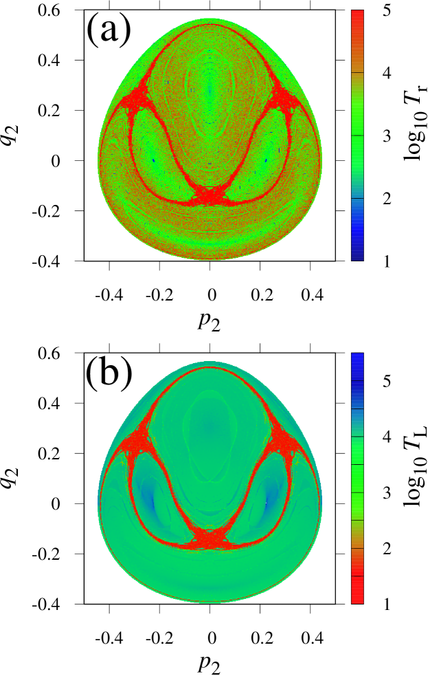
Figure 1: (a) The Poincaré recurrence chart for the Hénon–Heiles system, in the ($p_{2}$, $q_{2}$) plane, at $E=0.1$. Red colour corresponds to $T_{\mathrm{r}}>10^{5}$. (b) The Lyapunov time chart for the same system. Red colour corresponds to $T_{\mathrm{L}}<100$. In the both cases (a) and (b), the integration time $T_{\mathrm{int}}=10^{5}$.

Fig. 1 shows the ($p_{2}$, $q_{2}$) diagrams with the Poincaré recurrence and Lyapunov times indicated in a colour grade. The diagrams allow one to judge on the structure of the phase space of the Hénon–Heiles system. The Poincaré recurrence and Lyapunov times are calculated on a $500\times 500$ grid with $\approx 150000$ nodes inside the bounded phase space. In Fig. 1a, the Poincaré recurrence times $T_{\mathrm{r}}\leq 100$ (blue colour) correspond to the trajectories passing through the centers of various resonances or close to them. The Poincaré recurrence times $10^{2}<T_{\mathrm{r}}\leq 2\times 10^{4}$ (green colour) correspond to the librational trajectories far from centers of resonances. The Poincaré recurrence times $2\times 10^{4}<T_{\mathrm{r}}\leq 5\times 10^{4}$ (light red colour) correspond to the regular trajectories located far from the resonances, and also probably to weakly chaotic trajectories. The ring-like red areas all correspond to chaotic trajectories; they have $T_{\mathrm{r}}>10^{5}$.

To separate the trajectories into regular and chaotic ones, the method proposed in [3] is used. Its essence consists in the analysis of the modal structure of the differential distribution of the values of the computed Lyapunov exponents (in fact, finite-time local Lyapunov exponents) computed on a grid of initial data or values of parameters. Generally, the distribution has two peaks, one fixed and one moving when the computation time is increased. The fixed one corresponds to the chaotic trajectories. On the contrary, the peak corresponding to the regular trajectories moves along the horizontal axis towards smaller computed finite-time LE values (towards larger values of the Lyapunov times). Identifying the center of the gap between the peaks, one obtains a numerical criterion for separating the regular and chaotic trajectories.

In Fig. 1b, the Lyapunov times $T_{\mathrm{L}}<100$ (red colour) correspond to the chaotic trajectories. Most of the regular trajectories have $T_{\mathrm{L}}>10^{4}$ (blue colour). The trajectories with $10^{3}<T_{\mathrm{L}}<10^{4}$ (green colour) are also probably regular, but they are located close to separatrices of resonances. Note the good structural agreement between Fig. 1a and Fig. 1b, regarding the locations and sizes of the areas with the same character of dynamics.

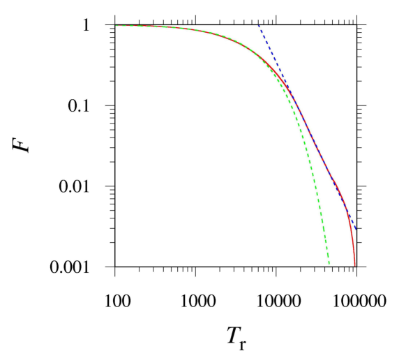
Figure 2: The integral distribution of the Poincaré recurrence times in the Hénon–Heiles system (the solid curve). The dashed curves represent fitting functions as explained in the text. The parameters and initial data are the same as in Fig. 1.

Fig. 2 shows the normalized integral distribution of the Poincaré recurrence times. The distribution subdivides into two parts: $T_{\mathrm{r}}\in[0,10^{4}]$ and $T_{\mathrm{r}}\in[2\times 10^{4},8\times 10^{4}]$. The first part is naturally fitted by the exponential function $F\propto\exp(-\alpha T_{\mathrm{r}})$, where $\alpha=1.5\times 10^{-4}$ (green dashed curve), and the second part is naturally fitted by the power-law function $F\propto{T_{\mathrm{r}}}^{-\beta}$, where $\beta=2.09$ (blue dashed straight line). In the both cases, the correlation coefficient for the fitting function is ${\cal R}=0.99$.

2.3 Implementation of the PRM_HH problem

The algorithm for calculating the Poincaré recurrence times for the considered system with a bounded phase space (namely, the Hénon–Heiles system) is implemented in the PRM_HH code, written in Fortran90. The total length of the code is only 180 lines (excluding the integrator).

To integrate the equations of motion, the Dormand–Prince integrator DOP853 [46], realizing the 8th order Runge–Kutta method with an automatic time step size control, is used. The maximum value of the time step size is set to $10^{-5}$, and the local error tolerance to $10^{-12}$.

The program consists of the main part (PRM_HH) and a subroutine (calc_rec_time). In the calc_rec_time, the DOP853 integrator is invoked, including subroutines fcn (where the equations of motion are defined) and solout (where the recurrence condition is checked after each integration step). Thus, in the PRM_HH main program loop, the subroutine calc_rec_time (t, t_end, y) is called, where y contains initial data for the integration.

INPUT. The parameters and initial conditions for the integration (the energy value, the initial data grid and the radius of the neighborhood of the initial point where the recurrence is fixed) are set directly in the PRM_HH program body. They are given by:

• H : the energy of the system; in the given problem, it takes values within $[0,1/6]$.

• EPS : the radius of the neighborhood (in which the Poincaré recurrence is fixed) of a point in the phase space.

• T = 0 and T_END specify the integration time interval.

• Q_2_INIT, Q_2_END, P_2_INIT, and P_2_END define the borders of a uniform grid of initial data in the plane ($p_{2}$, $q_{2}$).

• N_GRID : the number of steps along the axes $p_{2}$ and $q_{2}$.

OUTPUT. The output of the program PRM_HH is directed to the file rec_time.dat. The first and second columns in the file contain the initial conditions in the plane ($p_{2}$, $q_{2}$). The third column contains the recurrence time rec_time. If the integration time is too short to determine the recurrence time, the value of the upper limit of the integration time plus one is written to the third column.

Thus, at the end of the simulation, the PRM_HH code gives $N_{p_{2}}\times N_{q_{2}}=\mathrm{N\_GRID}\times\mathrm{N\_GRID}$ Poincaré recurrence time values.

2.4 The Poincaré recurrence method: the case of
non-bounded phase space

In the case of non-bounded phase space, the Poincaré recurrences are defined with respect to a neighbourhood of a starting point in the phase space and with respect to the “escape” separatrix (e.g., parabolic separatrix in the hierarchical restricted three-body problem).

Let us consider, as a representative paradigm, the circumbinary dynamics of a passively gravitating particle in the framework of the restricted planar three-body problem. The mass parameter is defined as $\mu=m_{2}/(m_{1}+m_{2})$, where $m_{1}\geq m_{2}$ are the masses of the primaries. The simulation is made in the synodic reference frame. The Hamiltonian of the problem is given by

$$H=\frac{1}{2}\left(P_{X}^{2}+P_{Y}^{2}\right)+YP_{X}-P_{Y}X-V(X,Y),$$ (2)

where $X$, $Y$ are the Cartesian barycentric coordinates of a passively gravitating tertiary and $P_{X}$, $P_{Y}$ are their conjugate momenta, $V(X,Y)$ is the gravitational potential (see, e.g., [1, 47]):

$$V(X,Y)=\frac{1-\mu}{R_{1}}+\frac{\mu}{R_{2}},$$ (3)

where $R_{1}=\left[\left(X-\mu\right)^{2}+Y^{2}\right]^{1/2}$ and $R_{2}=\left[\left(X+\left(1-\mu\right)\right)^{2}+Y^{2}\right]^{1/2}$.

We use the integration code with the Levi–Civita regularization (see [48, 49] for the equations). The number of the tertiary’s orbital revolutions serves to measure the first recurrence times.

To assess the PRM performance, we use two methods in parallel: the PRM and the LE methods. The PRM method is implemented in the PRM_3B code. The computation of orbits is based on a previous code used to compute phase space fractal structure of the dynamics governed by Hamiltonian (2) [50]. The integrator used is the DOP853 integrator [46], the same as described above in Subsection 2.3.

In the PRM, the first recurrence is fixed when the following conditions start to be satisfied:

$$X\in X_{0}\pm\Delta X,\quad Y\in Y_{0}\pm\Delta Y,\quad P_{X}\in P_{X_{0}}\pm\Delta P_{X},\quad P_{Y}\in P_{Y_{0}}\pm\Delta P_{Y},$$ (4)

where $X_{0},Y_{0},P_{X_{0}},P_{Y_{0}}$ are the initial conditions in the synodic reference frame, and $\Delta X=\Delta Y=\Delta P_{X}=\Delta P_{Y}=10^{-3}$. Thus, here the $\varepsilon$ neighbourhood is defined as a box, instead of a sphere used above in the Hénon–Heiles problem (Subsection 2.3).

We compute the dynamics on $201\times 201$ grid nodes in the plane “pericentric distance – eccentricity” ($q$–$e$) of the initial conditions for the tertiary. The PRM_3B code gives $201\times 201=40401$ values of the number of the orbital revolutions of the tertiary before the first recurrence.

The LE code computes the LE global charts. To compute the maximum Lyapunov exponent (in fact, the maximum finite-time local Lyapunov exponent), the code integrates the variational equations, simultaneously with the equations of motion. The code gives $201\times 201=40401$ values of the maximum Lyapunov exponent (the maximum finite-time local LE) after $T=10^{5}$ orbital revolutions of the binary.

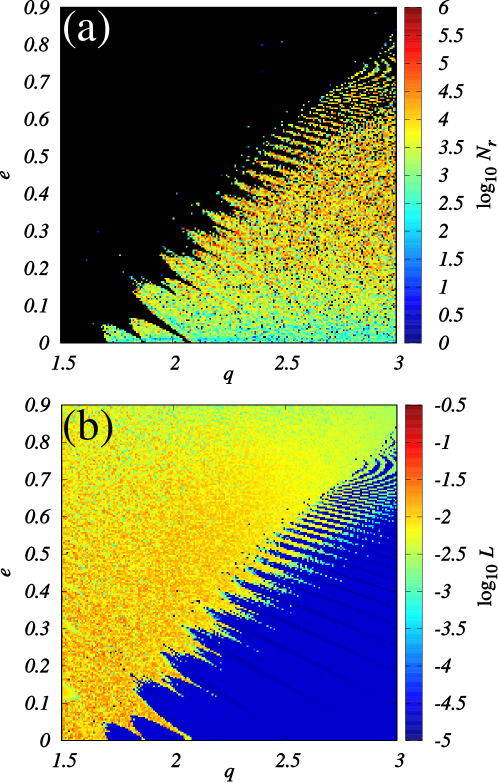
Figure 3: (a) The Poincaré recurrence chart in the ($q$, $e$) (“pericentric distance – eccentricity”) plane in the planar restricted three-body problem at $\mu=0.1$. $N_{r}$ is the number of the tertiary’s orbital revolutions before the recurrence. The integration time $T_{\mathrm{int}}=10^{6}$. Black colour corresponds to the orbits without recurrences within the integration time $T_{\mathrm{int}}$. (b) The Lyapunov time chart for the same system.

A comparison of the stability diagrams computed using the LE and PRM is presented in Figure 3. The choice of the ($q$, $e$) (“pericentric distance – eccentricity”) plane is justified by the dynamical nature of the problem; this choice is quite usual in problems concerning the circumbinary motion in celestial-mechanical systems [5]. The emergence of the “teeth” at the order/chaos boundary is due to the fractal resonant structure of the border; the most prominent teeth are formed by the overlap of subresonances of integer and half-integer mean motion resonances between the particle and the central gravitating binary (see [5]). A close agreement between the outcomes of application of the two methods is apparent.

2.5 Implementation of the PRM_3B problem

The algorithm for calculating the Poincaré recurrence times for a particular case of the unbounded phase space (namely, the restricted three-body problem) is implemented in the PRM_3B program written in Fortran90. The code length is $600$ lines (excluding the integrator).

Typically, the code makes a loop over $N_{e}$ initial values of the eccentricity $e$ for a fixed initial pericentric distance $q$. A Python code generates $N_{q}$ executables with different $q$.

The Levi–Civita regularization is employed to treat close encounters of the bodies. For each integration step, the regularization code invokes three changes of the reference frame. It takes $150$ lines. To integrate the equations of motion, the DOP853 integrator is used, the same as described above in Subsection 2.3.

INPUT. Several parameters are initially allocated to the PRM_3B code:

• N : the number of the computed particle trajectories.

• MU : the mass parameter.

• RMAX : the maximum size (radius) of the orbits. If a particle were going beyond this limit, it is regarded to have been ejected from the system.

• RMIN1 : the minimum radius around the mass $m_{1}$. If a particle were going below this limit, we assume a collision with $m_{1}$.

• RMIN2 : the same parameter as above, but for $m_{2}$.

• TMAX : the maximum time of simulation (counted in the binary’s orbital revolutions).

• TAU : the maximum allowed integration step size.

• EPS : the precision of the integration.

• EXMIN : the minimum initial eccentricity.

• EXMAX : the maximum initial eccentricity.

OUTPUT. At the end of the simulation, the PRM_3B code gives $N_{r}$ values of the number of the tertiary’s orbital revolutions before the first recurrence. The process is repeated $N_{q}$ times on different computer cores.

3 Poincaré recurrence statistics and diffusion rates

The average time of recurrence (to one and the same subset of phase space) can be roughly related in many cases (in particular, in the case of the standard map [51], describing an infinite set of interacting resonances) to the diffusion rate by the following formula

$$\tau\sim\frac{(\Delta y)^{2}}{D_{y}}$$ (5)

[38, p. 11–12], where $\tau$ is the mean recurrence time, $\Delta y$ is the characteristic distance in an appropriate variable, $D_{y}$ is the diffusion rate in this variable. In many-dimensional systems, a characteristic recurrence time can be roughly estimated by identifying the “slowest” (that exhibiting the slowest variation) variable in the system and, by applying Equation (5) for motion in this variable, assessing $\tau$.

Therefore, the average return time can be set to be equal to the average diffusion time. Formula (5) can be appropriate, as a simple but effective basic relation, in many applications. As soon as PRM allows one to construct charts of the diffusion timescales or rates, one can introduce a kind of the “dynamical temperature” [52] to characterize the global dynamical behaviour of any system under study.

The character of the distribution of Poincaré recurrences at large timescales is determined by the stickiness effect; generally, the decay is algebraic [38, 39, 40]. Starting with the pioneering work by Chirikov and Shepelyansky [38], the algebraic decay in the recurrence statistics in Hamiltonian systems with divided phase space was considered, in particular, in [38, 39, 41, 42, 43, 40]. Chirikov [41], using his resonant theory of critical phenomena in Hamiltonian dynamics, predicted the critical exponent $\alpha$ in the integral recurrence distribution

$$F(T_{\rm r})\propto T_{\rm r}^{-\alpha}$$ (6)

to be equal to 3/2. (The integral distribution function $F(T_{\rm r})$ is defined as the fraction of the recurrences that have the duration greater than $T_{\rm r}$.)

In massive numerical simulations of dynamics of various Hamiltonian systems, the algebraic decay was explored in [43]. System-dependent power-law exponents were revealed; however, the “universal” average exponent turned out to be well-defined: $\alpha=1.57\pm 0.03$ [43]. This is quite close to the theoretical $3/2$ value cited above. In celestial mechanics, the algebraic decay was revealed in numerical experiments on chaotic asteroidal dynamics [53, 54]. It was found that the tail of the integral distribution of the time intervals $T_{\rm r}$ between jumps of the eccentricity of asteroids in the vicinity of the 3/1 mean-motion resonance with Jupiter is algebraic:

$$F\propto T_{\rm r}^{-\alpha},$$ (7)

where $\alpha\approx 1.5$–$1.7$.

Local properties of chaotic diffusion in Hamiltonian systems were studied in [55]; the statistics of exit times from high-order resonances were explored in [56]. In the both studies, the results are in agreement with the Greene–MacKay theory [57, 58] of the critical golden curve. The longest Poincaré recurrences were obtained in [59]. As in [43], it was concluded that the longest recurrences originate from non-golden islands.

Thus, the power-law statistical relations between $T_{\mathrm{L}}$ and $T_{\mathrm{r}}$ are expected to emerge on long timescales, when sticking of trajectories to chaos borders starts to dominate in the statistics (see discussion in [60]; also see figure 6 in [61], or figures 1 and 2 in [60]). The relationship between the recurrence times $T_{\rm r}$ and the Lyapunov times $T_{\rm L}$ in systems with the stickiness effect is generally quadratic [60, 62]. Note that the long-term recurrence distributions, as well as relationships between $T_{\rm r}$ and $T_{\rm L}$, in systems with non-bounded phase space where escapes are possible, can have various power-law indices, though their algebraic form is sustained [62].

In the current study, we have used relatively short computation times — short enough to fix most of the first recurrences on a given grid. On much longer timescales, when sticking phenomena come into play and recurrence statistics can be potentially gathered for each node on the grid, comparisons between PRM and LE charts, made in parallel, can be employed to establish and massively study statistical $T_{\rm L}$–$T_{\rm r}$ relationships; that is why any application of the LE and PRM methods in parallel can be of particular interest.

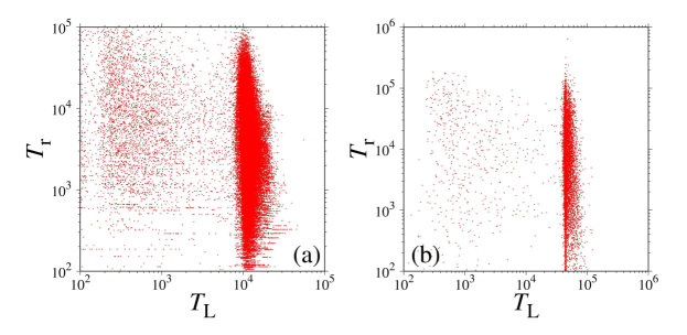
Figure 4: The relationships between the Lyapunov and Poincaré recurrence times in the considered systems: the Hénon–Heiles system (a) and the three-body problem (b).

In Fig. 4, correlation plots “$T_{\mathrm{L}}$–$T_{\mathrm{r}}$” (Lyapunov time – recurrence time) for the both systems considered in this article are presented. They have been constructed for the same data that were computed to construct the PR charts, in such a way: for a trajectory starting at a point in a PR chart, $T_{\mathrm{L}}$ is fixed at the time $T_{\mathrm{r}}$ when the first recurrence is fixed; the set of ($T_{\mathrm{L}}$, $T_{\mathrm{r}}$) points over all initial data forms the correlation plot. In fact, the both “$T_{\mathrm{L}}$–$T_{\mathrm{r}}$” plots show no correlation (only broad scatter, apart from the vertical pile-ups corresponding to regular trajectories), but one should not expect any straightforward correlation between $T_{\mathrm{L}}$ and $T_{\mathrm{r}}$ here, as soon as they are restricted by a relatively small time limit of the computation. Besides, as discussed above, the nature of emerging correlations, if any, can be rather diverse and non-rigorous; see also [63, 64]. Therefore, PR charts have an independent value, in this sense: they cannot be reproduced by any transformation of LE data.

As soon as relatively small time limits are set for the computation of PR charts, sticking phenomena are relatively unimportant. Besides, the measure of the critical component (where the sticking occurs) of the phase space is also usually small (see [41]); therefore, it does not affect the quality of PR charts.

4 Discussion

The assumption on the Euclidean metric to define the neighbourhood where recurrences are fixed has been made throughout the article, but other possibilities exist and they can be studied in the course of the further development of the method.

Note that for the angle variables, the interval of variation (normally $2\pi$), in the current algorithm version is divided in the same proportion as the intervals of variation of the momentum variables with respect to the approximate size of the (bounded) phase space in the momentum variables.

A key point in the both considered cases of bounded and unbounded phase space is the choice of the size $\varepsilon$ of the “recurrence-fixing sphere” (i.e., the neighbourhood of the initial point, where the recurrences are fixed) at a given computation time; or, alternatively, a lower time limit for the computation time, given the size $\varepsilon$.

For a bounded phase space, the lower time limit can be roughly estimated assuming the approximate ergodicity of the chaotic motion (excluding the critical component, which has low measure, as noted above): $\Delta t/t_{\mathrm{comp}}\approx\Delta V/V_{\mathrm{s}}\sim\varepsilon^{n}/V_{\mathrm{s}}$, where $\Delta t$ is the time of residence of the trajectory in a point’s neighbourhood where recurrences are fixed, $t_{\mathrm{comp}}$ is the time of computation, $V_{\mathrm{s}}$ is the full volume of the phase space, $\Delta V\sim\varepsilon^{n}$ is the the volume of the $\varepsilon$-box where recurrences are fixed, and $n$ is the dimension of the phase space. Therefore, the minimum computation time, allowing for at least a single expected recurrence, is $\sim V_{\mathrm{s}}/\varepsilon^{n}$, in time steps of integration (assuming the step is constant).

However, in practice, an appropriate time of computation is easily evaluated empirically, by trying its higher and higher values until the PR chart becomes noiseless.

Alternatively, an effective $\varepsilon$ can be easily evaluated by fine-tuning the needed resolution of a dynamical chart of a system under study. The algorithm is as follows: at first the size of the recurrence-fixing sphere or box is chosen corresponding to the desired resolution of a constructed stability diagram or phase portrait; then, the computations are performed on a timescale of at least one magnitude greater than the duration of the first-fixed (over all the grid) recurrence. If this timescale cannot be achieved using available computer resources, the desired resolution should be decreased.

The novel PRM and the custom LE methods can be used in concert, so that to utilize the best properties of both; when the computation time is long enough for the sticking phenomenon to come into play, such an approach would allow one to use statistical relationships between the Lyapunov and diffusion timescales, when making predictions for the long-term qualitative dynamical behaviour.

It should be underlined that the global charts of the massively computed Poincaré recurrence times provide direct global representations of spatial distributions of the local diffusion times. The charts constructed in the quantities inverse to the recurrence times provide massive measures of the local diffusion rates, thus giving the picture of the global behaviour of the dynamical temperature (defined analogously as in [52]) of any system under study.

Finally, note that for all examples provided in this article, the integrator time step upper limit (set to $10^{-5}$ for PRM_HH and $2\pi\times 10^{-3}$ for PRM_3B) is small enough so that there is no need, as established empirically, for any step diminishing whenever the trajectory approaches a desired neighborhood. Besides, in our computations, the local error tolerance of the Dormand–Prince integrator was set to $10^{-12}$ for PRM_HH (and $10^{-10}$ for PRM_3B), thus smaller than the chosen $\varepsilon$ values by many orders of magnitude, therefore, the integrator accuracy was by far sufficient. Due to the essential sensitivity of the chaotic motion to the initial conditions, nearby initial conditions may give rather different PR times. However, on fine enough grids of initial data, the corresponding “noise” in the PR charts is suppressed, due to the statistical averaging of the effect.

In this article, we have concentrated on the Hamiltonian systems. Extensions of the method to the realm of dissipative systems might be warranted; we leave this promising possibility for a future work. Note also that the PRM can be developed further on to incorporate calculations of second and consecutive recurrences. This may favor to suppress any “noisy” appearances in PRM diagrams. This opportunity is also left for a future analysis.

5 Conclusions

We have shown that the novel PRM and the custom LE methods expose the global dynamics almost identically, but the PRM allows one to construct, in some approximation, charts of diffusion rates. This ability reveals the major advantage of the novel method over the custom global numerical tools (LE, FLI, MEGNO, FA). Moreover, it is algorithmically simple and straightforward to apply.

References

- [1] A. Morbidelli, Modern Celestial Mechanics. Aspects of Solar System Dynamics. Taylor and Francis, Padstow, UK, 2002.
- [2] N.P. Maffione, L.A. Darriba, P.M. Cincotta, C.M. Giordano, Mon. Not. R. Astron. Soc. 429 (2013) 2700–2717.
- [3] A.V. Melnikov, I.I. Shevchenko, Solar System Research 32 (1998) 480–490.
- [4] I.I. Shevchenko, A.V. Melnikov, JETP Lett. 77 (2003) 642–646.
- [5] E.A. Popova, I.I. Shevchenko, Astrophys. J. 769 (2013) 152.
- [6] J. Lages, I.I. Shevchenko, D.L. Shepelyansky, Astron. J. (2017) 153–272.
- [7] J. Lages, I.I. Shevchenko, G. Rollin, Icarus 307 (2018) 391–399.
- [8] E. Pilat-Lohinger, R. Dvorak, Celest. Mech. Dyn. Astron. 82 (2002) 143–153.
- [9] P.M. Cincotta, C. Simó, Astron. Astrophys. Suppl. 147 (2000) 205–228.
- [10] P.M. Cincotta, C.M. Giordano, C. Simó, Physica D 182 (2003) 151–178.
- [11] A.C.M. Correia, S. Udry, M. Mayor, W. Benz, J.-L. Bertaux, F. Bouchy, J. Laskar, C. Lovis, C. Mordasini, F. Pepe, D. Queloz, Astron. Astrophys. 496 (2009) 521–526.
- [12] J. Laskar, A.C.M. Correia, Astron. Astrophys. 496 (2009) L5–L8.
- [13] V.I. Oseledec, Transactions of the Moscow Mathematical Society 19 (1968) 197–231.
- [14] G. Benettin, L. Galgani, J.-M. Strelcyn, Phys. Rev. A. 14 (1976) 2338–2345.
- [15] G. Benettin, L. Galgani, A. Giorgilli, J.-M. Strelcyn, Meccanica 15 (1980) 9–30.
- [16] H.F. von Bremen, F.E. Udwadia, W. Proskurowski, Physica D 101 (1997) 1–16.
- [17] G. Tancredi, A. Sánchez, F. Roig, Astron. J 121 (2001) 1171–1179.
- [18] N.V. Kuznetsov, G.A. Leonov, T.N. Mokaev, A. Prasad, M.D. Shrimali, Nonlinear Dynamics 92 (2018) 267–285.
- [19] I.I. Shevchenko, V.V. Kouprianov, Astron. Astrophys. 394 (2002) 663–674.
- [20] C. Froeschlé, E. Lega, R. Gonczi, Celest. Mech. Dyn. Astron. 67 (1997) 41–62 .
- [21] D. D. Carpintero, N. Maffione, L. Darriba, Astron. and Comp. 5 (2014) 19–27.
- [22] J. Laskar, Icarus 88 (1990) 266–291.
- [23] J. Laskar, Physica D 67 (1993) 257–281.
- [24] J. Laskar, arXiv: math/0305364 (2003).
- [25] M. Valluri, V. P. Debattista, T. Quinn, B. Moore, Mon. Not. R. Astron. Soc. 403 (2010) 525–544.
- [26] M. Valluri, V. P. Debattista, T. R. Quinn, R. Roškar, J. Wadsley, Mon. Not. R. Astron. Soc. 419 (2012) 1951–1969.
- [27] R. Dvorak, E. Pilat-Lohinger, R. Schwarz, F. Freistetter, Astron. Astrophys. 426 (2004) L37–L40.
- [28] R. Schwarz, N. Haghighipour, S. Eggl, E. Pilat-Lohinger, B. Funk, Mon. Not. R. Astron. Soc. 414 (2011) 2763–2770.
- [29] M.J. Holman, P.A. Wiegert, Astron. J. 117 (1999) 621–628.
- [30] E. Pilat-Lohinger, B. Funk, R. Dvorak, Astron. Astrophys. 400 (2003) 1085–1094.
- [31] F. Panichi, K. Goździewski, G. Turchetti, Mon. Not. R. Astron. Soc. 468 (2017) 469–491.
- [32] H. Poincaré, Acta Math. 13 (1890) 1–270.
- [33] V.I. Arnold, Mathematical Methods of Classical Mechanics. Springer-Verlag, New York, 1989.
- [34] N. Marwan, M.C. Romano, M. Thiel, J. Kurths, Physics Reports 438 (2007) 237–329.
- [35] N. Marwan, European Physical Journal Special Topics 164 (2008) 3–12.
- [36] N. Asghari, C. Broeg, L. Carone, et al., Astron. Astrophys. 426 (2004) 353–365.
- [37] C. Manchein, M.W. Beims, Phys. Lett. A 377 (2013) 789–793.
- [38] B.V. Chirikov, D.L. Shepelyansky, Statistics of Poincaré recurrences and the structure of the stochastic layer of the non-linear resonance. PPPL-TRANS-133 (1981). INP Preprint 81–69. Institute of Nuclear Physics, Novosibirsk, 1981.
- [39] B.V. Chirikov, D.L. Shepelyansky, Physica D 13 (1984) 395–400.
- [40] D.L. Shepelyansky, Phys. Rev. E 82 (2010) 055202(R).
- [41] B.V. Chirikov, Patterns in chaos, INP Preprint 90–109, Institute of Nuclear Physics, Novosibirsk, 1990.
- [42] B.V. Chirikov, Poincaré recurrences in microtron and the global critical structure, INP Preprint 99–7, Institute of Nuclear Physics, Novosibirsk, 1999; eprint arXiv:nlin/0006013.
- [43] G. Cristadoro, R. Ketzmerick, Phys. Rev. Lett. 100 (2008) 184101.
- [44] E.J. Ngamga, D.V. Senthilkumar, A. Prasad, P. Parmananda, N. Marwan, J. Kurths, Phys. Rev. E 85 (2012) 026217.
- [45] M. Hénon, C. Heiles, Astron. J. 69 (1964) 73–79.
- [46] E. Hairer, S.P. Nørsett, G. Wanner, Solving Ordinary Differential Equations I. Nonstiff Problems. Springer–Verlag, Berlin, 1993.
- [47] C.D. Murray, S. Dermott, Solar System Dynamics. Cambridge University Press, Cambridge, 1999.
- [48] A. Celletti, Stability and chaos in celestial mechanics, Springer–Verlag, Berlin, Heidelberg, 2010.
- [49] A. Celletti, Singularities in gravitational systems: Applications to chaotic transport in the Solar system, Springer–Verlag, Berlin, Heidelberg, 2002.
- [50] G. Rollin, J. Lages, D.L. Shepelyansky, New Astronomy 47 (2016) 97–104.
- [51] B.V. Chirikov, Phys. Rep. 52 (1979) 263–379.
- [52] I.I. Shevchenko, Physica A 386 (2007) 85–91.
- [53] I.I. Shevchenko, H. Scholl, in: “Dynamics, ephemerides and astrometry of the Solar system,” edited by S. Ferraz-Mello, B. Morando, J.-E. Arlot, Kluwer, Dordrecht, 183, 1996.
- [54] I.I. Shevchenko, H. Scholl, Celest. Mech. Dyn. Astron. 68 (1997) 163–175.
- [55] S. Ruffo, D.L. Shepelyansky, Phys. Rev. Lett. 76 (1996) 3300–3303.
- [56] B.V. Chirikov, D.L. Shepelyansky, Phys. Rev. Lett. 82 (1999) 528–531.
- [57] J.M. Greene, J. Math. Phys. 20 (1979) 1183–1201.
- [58] R.S. MacKay, Physica D 7 (1983) 283–300.
- [59] K.M. Frahm, D.L. Shepelyansky, Eur. Phys. J. B 86 (2013) 322.
- [60] I.I. Shevchenko, Phys. Lett. A 241 (1998) 53–60.
- [61] N. Murray, M. Holman, Astron. J. 114 (1997) 1246–1259.
- [62] I.I. Shevchenko, Phys. Rev. E 81 (2010) 066216-1-11.
- [63] A. Morbidelli, C. Froeschlé, Celest. Mech. Dyn. Astron. 63 (1996) 227–239.
- [64] M.S. Baptista, E.J. Ngamga, P.R.F. Pinto, M. Brito, J. Kurths, Phys. Lett. A 374 (2010) 1135–1140.