Fast, accurate simulation of polaron dynamics and multidimensional spectroscopy by multiple Davydov trial states

Abstract

By employing the Dirac-Frenkel time-dependent variational principle, we study the dynamical properties of the Holstein molecular crystal model with diagonal and off-diagonal exciton-phonon coupling. A linear combination of the Davydov D₁ (D₂) Anstaz, referred to as the “multi-D₁ Ansatz” (“multi-D₂ Ansatz”), is used as the trial state with enhanced accuracy but without sacrificing efficiency. The time evolution of the exciton probability is found to be in perfect agreement with that of the hierarchy equations of motion, demonstrating the promise the multiple Davydov trial states hold as an efficient, robust description of dynamics of complex quantum systems. In addition to the linear absorption spectra computed for both diagonal and off-diagonal cases, for the first time, $2$D spectra have been calculated for systems with off-diagonal exciton-phonon coupling by employing the multiple ${\rm D}_{2}$ Ansatz to compute the nonlinear response function, testifying to the great potential of the multiple ${\rm D}_{2}$ Ansatz for fast, accurate implementation of multidimensional spectroscopy. It is found that the signal exhibits a single peak for weak off-diagonal coupling, while a vibronic multi-peak structure appears for strong off-diagonal coupling.

I Introduction

Thanks to recent advances in ultrafast spectroscopy, femtosecond photoexcitation has became a major technique in probing elementary excitations, which brought about numerous studies on relaxation dynamics of photoexcited entities, for example, polarons in inorganic liquids and solids an_04 ; zheng_06 ; liu_06 , charge carriers in topological insulators bron_14 ; tim_12 , trapped electrons and holes in the semiconductor nanoparticles chi_02 ; kli_00 ; kim_96 , and electron-hole pairs in light-harvesting complexes of photosynthesis sau_79 ; reng_01 ; blan_02 ; gron_06 ; LP_Molecule . Emerging technological capabilities to control femtosecond pulse durations and down-to-one-hertz bandwidth resolutions offer unpreceded windows on vibrational dynamics and excitation relaxation. For example, progress in femtosecond spectroscopy has enabled the observation of a coherent phonon wave packet oscillating along an adiabatic potential surface associated with a self-trapped exciton in a crystal with strong exciton-phonon interactions tom_00 . Taking advantage of the ultrashort pulse widths of recent lasers, the femtosecond dynamics of polaron formation and exciton-phonon dressing have been observed in pump-probe experiments dex_00 ; sug_01 ; mor_10 . These experiments have revealed a complex interplay between a single exciton and its surrounding phonons under nonequilibrium conditions, while theoretical developments have not been kept in parallel. In particular, modeling of polaron dynamics have not received much-deserved attention over the last six decades ale_95 ; pee_84 .

From a theoretical point of view, capturing time-dependent polaron formation requires an in-depth understanding of the combined dynamics of the particle and the phonons in its environment ran_06 . A simple Hamiltonian is that of the extended Holstein molecular crystal model hol_59 ; hol_59_2 with simultaneous diagonal and off-diagonal exciton-phonon coupling, as shown in Fig. 1(a), where the diagonal coupling represents a nontrivial dependence of the exciton site energies on the lattice coordinates, and the off-diagonal coupling, a nontrivial dependence of the exciton transfer integral on the lattice coordinates su_79 ; dis_84 ; sumi_89 ; zhao_94 ; dmchen_11 . A large body of literature exists on the study of the conventional form of the Holstein Hamiltonian with the diagonal coupling only luo_10 ; sun_10 . It seems fundamental to take into account simultaneously diagonal and off-diagonal coupling to characterize solid-state excimers dis_84 ; sumi_89 as a variety of experimental and theoretical studies imply a strong dependence of electronic tunneling upon certain coordinated distortions of neighboring molecules in the formation of bound excited states. However, complete understanding of the off-diagonal coupling and out-of-equilibrium phenomena remains elusive. Early treatments of the off-diagonal coupling include the Munn-Silbey theory MunnSilbey ; zhao_94 ; dmchen_11 , which is based upon a perturbative approach with additional constraints on canonical transformation coefficients determined by a self-consistency equation. The global-local (GL)Ansatz zhao_94b ; zhao_08 , formulated by Zhao and co-workers in the early $1990$s, was subsequently employed in combination with the dynamic coherent potential approximation (with the Hartree approximation) to arrive at a state-of-the-art ground-state wave function as well as higher eigenstates liu_09 .

Because an exact solution of the polaron dynamic still eludes us, several numerical approaches have been developed. For example, the time-dependent Schrödinger equation can be numerically integrated in real space for a few phonon time periods to probe the time evolution of electron and phonon densities and electron-phonon correlation functions ku_07 . However, the method is time consuming and impractical when the size of the system is large. Fortunately, time-dependent variational approaches are still valid to treat the polaron dynamics in such cases as long as a proper trial wave function is adopted. Previously, static properties of the Holstein polaron were studied by Zhao and his co-workers with a set of trial wave functions based upon phonon coherent states, including the Toyozawa Ansatz zhao_94b ; meier_97 ; zhao_97 , the GL Ansatz zhao_94b ; zhao_97 ; zhao_08 ; zhao_97b , a delocalized form of the Davydov $\rm D_{1}$ Ansatz sun_13 , and the multi-$\rm D_{1}$ Ansatz zhou_14 . The results of these extended Davydov Ansätze exhibit great promises in the investigation of the polaron energy band and other static properties of the Holstein polaron. However, difficulties surround accurate simulations of the polaron dynamics from an arbitrary initial state, such as a localized state for which the aforementioned Bloch states are not well suited. Thus, the question of what type of the variational trial state is suitable for the polaron dynamics of the Holstein model is still open.

By using the Dirac-Frenkel time-dependent variational principle, a powerful apparatus to reveal accurate dynamics of quantum many-body systems dira_30 , one can study the polaron dynamics of the Holstein model with the simultaneous diagonal and off-diagonal exciton-phonon coupling. Time-dependent variational parameters, which specify the trial state, are obtained by solving a set of coupled differential equations generated from the Lagrangian formalism of the Dirac-Frenkel variation. Validity of the trial states is carefully examined by quantifying how faithfully they follow the Schrödinger equation luo_10 ; sun_10 ; zhao_12 . The hierarchy of the Davydov Ansätze includes two trial states of varying sophistication, referred to as the $\rm D_{1}$ and $\rm D_{2}$ Ansätze Davydov1 ; Davydov2 ; skri_88 ; for_93 ; han_94 , with the latter being a simplified version of the former. The ${\rm D_{1}}$ Ansatz is sufficient to describe the Holstein polaron dynamics with the diagonal coupling, but fails in the presence of the off-diagonal coupling. In comparison, the ${\rm D_{2}}$ Ansatz exhibits a nice dynamical performance with the off-diagonal coupling, though the deviation from the exact solution to the Schrödinger dynamics is not disregarded zhao_12 . Instead, superposition of the ${\rm D_{1}}$ or the ${\rm D_{2}}$ Ansatz will be adopted in our work, which offers significant improvements in the flexibility of the trial state zhou_15 , thus yielding accurate polaron dynamics of the Holstein model with the simultaneous diagonal and off-diagonal coupling.

Recently, two dimensional (2D) electronic spectroscopy has been widely used to probe ultrafast energy transfer and charge separation processes in photosynthetic light harvesting complexes Brixner ; Engel ; Collini ; Panitchayangkoon ; Myers ; Lewis ; Romero . Compared to linear spectroscopy techniques in which the spectral lines are often congested, ultrafast non-linear spectroscopies can resolve dynamical processes with various time scales. In a 2D electronic spectroscopy experiment and apparatus, for example, three ultra-short laser pulses, separated by two time delays, namely, the coherence time and the waiting time, are incident on the sample, and the resultant signal field is spectrally resolved in a given phase-matched direction. The 2D contour plots of the signals provide direct information about excitonic relaxation and dephasing in a variety of molecular systems. Simulation of 2D electronic spectra of molecular aggregates was previously carried out for the Holstein model with diagonal exciton-phonon coupling. However, the effect of off-diagonal coupling on the 2D spectra is yet to be addressed.

In this paper, the multiple Davydov trial states, called the multi-$\rm D_{1}$ and multi-$\rm D_{2}$ Ansätze, will be adopted to simulate the polaron dynamics of an extended Holstein Hamiltonian that includes the off-diagonal exciton-phonon coupling. Validity of these trial states is carefully examined with the linear absorption spectra compared closely with the ground-state energy band. In addition, 2D spectra for systems with off-diagonal exciton phonon coupling will be calculated by employing the multiple $\mathrm{D}_{2}$ Ansatz. The remainder of the paper is organized as follows. In Sec. II we introduce the Holstein Hamiltonian and two novel variational wave functions on the basis of the multiple Davydov trial states, together with a criterion that quantifies the deviation of our trial states from the solution to the Schrödinger equation. In Sec. III, results are analyzed including the time evolution of the exciton amplitudes and the phonon displacements, the quantitative measurement for the trial state validity, and the linear absorption and 2D spectra. Finally, conclusions are drawn in Sec. IV.

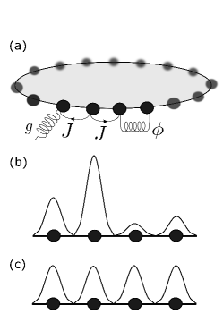
Figure 1: (a) Schematic of the Holstein ring. A simplified molecular crystal is treated as a ring where each point represents a big molecule and wave lines inside denote the phonons. (b) and (c) Schematics of waveshapes for the Davydov $\rm D_{1}$ and $\rm D_{2}$ Ansätze, respectively. The phonon part of the $\rm D_{1}$ Ansatz depends on both sites and momentum, while that of the $\rm D_{2}$ Ansatz is site independent.

II METHODOLOGY

II.1 Model

The Hamiltonian of the one-dimensional Holstein polaron is composed of

$$\hat{H}=\hat{H}_{\rm ex}+\hat{H}_{\rm ph}+\hat{H}_{\rm ex-ph}^{\rm diag}+\hat{H}_{\rm ex-ph}^{\rm o.d.}$$ (1)

where $\hat{H}_{\rm ex},\hat{H}_{\rm ph},\hat{H}_{\rm ex-ph}^{\rm diag}$ and $\hat{H}_{\rm ex-ph}^{\rm o.d.}$ represent the exciton Hamiltonian, bath (phonon) Hamiltonian, diagonal exciton-phonon coupling Hamiltonian and off-diagonal coupling Hamiltonian, respectively, which are defined as

$$\hat{H}_{\rm ex} = -J\sum_{n}\hat{a}_{n}^{\dagger}\left(\hat{a}_{n+1}+\hat{a}_{n-1}\right),$$

$$\hat{H}_{\rm ph} = \sum_{q}\omega_{q}\hat{b}_{q}^{\dagger}\hat{b}_{q},$$ (2)

$$\hat{H}_{\rm ex-ph}^{\rm diag} = -g\sum_{n,q}\omega_{q}\hat{a}_{n}^{\dagger}\hat{a}_{n}\left(e^{iqn}\hat{b}_{q}+e^{-iqn}\hat{b}_{q}^{\dagger}\right),$$

$$\hat{H}_{\rm ex-ph}^{\rm o.d.} = \frac{1}{2}\phi\sum_{n,q}\omega_{q}\{\hat{a}_{n}^{\dagger}\hat{a}_{n+1}[e^{iqn}(e^{iq}-1)\hat{b}_{q}+{\rm H.c.}],$$

$$+\hat{a}_{n}^{\dagger}\hat{a}_{n-1}[e^{iqn}(1-e^{-iq})\hat{b}_{q}+{\rm H.c.}]\},$$

where $\rm H.c.$ denotes the Hermitian conjugate, $\omega_{q}$ is the phonon frequency with momentum $q$, $\hat{a}_{n}^{{\dagger}}$ ($\hat{a}_{n}$) is the exciton creation (annihilation) operator for the $n$-th molecule, and $\hat{b}_{q}^{{\dagger}}$ ($\hat{b}_{q}$) is the creation (annihilation) operator of a phonon with the momentum $q$,

$$\hat{b}_{q}^{{\dagger}}=N^{-1/2}\sum_{n}e^{iqn}\hat{b}_{n}^{{\dagger}},\quad\hat{b}_{n}^{{\dagger}}=N^{-1/2}\sum_{q}e^{-iqn}\hat{b}_{q}^{{\dagger}}.$$ (3)

The parameters $J,g$ and $\phi$ represent the transfer integral, diagonal and off-diagonal coupling strengthes, respectively, and $N=16$ is the number of sites in the Holstein ring. In this paper, a linear phonon dispersion is assumed,

$$\omega_{q}=\omega_{0}\left[1+W(\frac{2\left|q\right|}{\pi}-1)\right],$$ (4)

where $\omega_{0}$ denotes a central phonon frequency, $W$ is the band width falling between $0$ and $1$, and $q=2\pi l/N$ represents the momentum index with $l=-\frac{N}{2}+1,\ldots,\frac{N}{2}$.

II.2 Multiple Davydov trial states

In the past, two typical Davydov trial states, i.e., the $\rm D_{1}$ and $\rm D_{2}$ Ansätze, were used to obtain the time evolution of the Holstein polaron following the Dirac-Frenkel variation scheme. The $\rm D_{2}$ Ansatz is a simplified version of the $\rm D_{1}$ Ansatz, since the phonon displacements of the $\rm D_{1}$ ($\rm D_{2}$) trial state is site-dependent (site-independent), as illustrated in Figs. 1(b) and (c). Multiple Davydov trial state with the multiplicity $M$ are then introduced in this paper, which can be constructed as follows

$$\left|{\rm D_{1}^{M}}\left(t\right)\right\rangle=\sum_{i}^{M}\sum_{n}^{N}\psi_{i,n}\left|n\right\rangle\left|\lambda_{i,n}\right\rangle,$$ (5)

$$=\sum_{i}^{M}\sum_{n}^{N}\psi_{i,n}\hat{a}_{n}^{\dagger}\left|0\right\rangle_{\rm ex}\exp\left\{\sum_{q}\left[\lambda_{inq}\hat{b}_{q}^{\dagger}-\lambda_{inq}^{\ast}\hat{b}_{q}\right]\right\}\left|0\right\rangle_{\rm ph},$$

and

$$\left|{\rm D_{2}^{M}}\left(t\right)\right\rangle=\sum_{i}^{M}\sum_{n}^{N}\psi_{i,n}\left|n\right\rangle\left|\lambda_{i}\right\rangle,$$ (6)

$$=\sum_{i}^{M}\sum_{n}^{N}\psi_{i,n}\hat{a}_{n}^{\dagger}\left|0\right\rangle_{\rm ex}\exp\left\{\sum_{q}\left[\lambda_{iq}\hat{b}_{q}^{\dagger}-\lambda_{iq}^{\ast}\hat{b}_{q}\right]\right\}\left|0\right\rangle_{\rm ph},$$

where $\psi_{i,n}$ and $\lambda_{inq}$ are related to the exciton probability and the phonon displacement, respectively, $n$ represents the site number in the molecular ring, and $i$ labels the coherent superposition state. If $M=1$, both the $|\rm D_{1}^{M}(t)\rangle$ and $|\rm D_{2}^{M}(t)\rangle$ Ansätze are restored to the usual Davydov $\rm D_{1}$ and $\rm D_{2}$ trial states, respectively. The equation of motion of the variational parameters $\psi_{i,n}$ and $\lambda_{inq}$ are then derived by adopting the Dirac-Frenkel variational principle,

$$\frac{d}{dt}\left(\frac{\partial L}{\partial\dot{\psi_{i,n}^{\ast}}}\right)-\frac{\partial L}{\partial\psi_{i,n}^{\ast}} = 0,$$

$$\frac{d}{dt}\left(\frac{\partial L}{\partial\dot{\lambda_{inq}^{\ast}}}\right)-\frac{\partial L}{\partial\lambda_{inq}^{\ast}} = 0.$$ (7)

For the multi-$\rm D_{1}$ Ansatz defined in Eq. (5), the Lagrangian $L_{1}$ is given as

$$L_{1} = \left\langle{\rm D}^{M}_{1}\left(t\right)\right|\frac{i\hslash}{2}\frac{\overleftrightarrow{\partial}}{\partial t}-\hat{H}\left|{\rm D}^{M}_{1}\left(t\right)\right\rangle$$ (8)

$$= \frac{i\hslash}{2}\left[\left\langle{\rm D}^{M}_{1}\left(t\right)\right|\frac{\overrightarrow{\partial}}{\partial t}\left|{\rm D}^{M}_{1}\left(t\right)\right\rangle-\left\langle{\rm D}_{1}\left(t\right)\right|\frac{\overleftarrow{\partial}}{\partial t}\left|{\rm D}^{M}_{1}\left(t\right)\right\rangle\right]$$

$$-\left\langle{\rm D}^{M}_{1}\left(t\right)\right|\hat{H}\left|{\rm D}^{M}_{1}\left(t\right)\right\rangle,$$

where the first term yields

$$\left\langle{\rm D}_{1}^{M}\left(t\right)\right|\frac{\overrightarrow{\partial}}{\partial t}\left|{\rm D}_{1}^{M}\left(t\right)\right\rangle-\left\langle{\rm D}_{1}^{M}\left(t\right)\right|\frac{\overleftarrow{\partial}}{\partial t}\left|{\rm D}_{1}^{M}\left(t\right)\right\rangle$$

$$=\sum_{i,j}^{M}\sum_{n}\left(\psi_{jn}^{\ast}\dot{\psi}_{in}-\dot{\psi}_{jn}^{\ast}\psi_{in}\right)S_{ji}$$

$$+\sum_{i,j}^{M}\sum_{n}\psi_{jn}^{\ast}\psi_{in}S_{ji}\sum_{q}\left[\frac{\dot{\lambda}_{jnq}^{\ast}\lambda_{jnq}+\lambda_{jnq}^{\ast}\dot{\lambda}_{jnq}}{2}\right.$$

$$\left.-\frac{\dot{\lambda}_{inq}\lambda_{inq}^{\ast}+\lambda_{inq}\dot{\lambda}_{inq}^{\ast}}{2}+\lambda_{jnq}^{\ast}\dot{\lambda}_{inq}-\lambda_{inq}\dot{\lambda}_{jnq}^{\ast}\right],$$ (9)

and the second term is

$$\left\langle{\rm D}^{M}_{1}\left(t\right)\right|\hat{H}\left|{\rm D}^{M}_{1}\left(t\right)\right\rangle$$

$$=\left\langle{\rm D}^{M}_{1}\left(t\right)\right|\hat{H}_{\rm ex}\left|{\rm D}^{M}_{1}\left(t\right)\right\rangle+\left\langle{\rm D}^{M}_{1}\left(t\right)\right|\hat{H}_{\rm ph}\left|{\rm D}^{M}_{1}\left(t\right)\right\rangle$$

$$+\left\langle{\rm D}^{M}_{1}\left(t\right)\right|\hat{H}_{\rm ex-ph}^{\rm diag}\left|{\rm D}^{M}_{1}\left(t\right)\right\rangle+\left\langle{\rm D}^{M}_{1}\left(t\right)\right|\hat{H}_{\rm ex-ph}^{\rm o.d.}\left|{\rm D}^{M}_{1}\left(t\right)\right\rangle.$$

Detailed derivations on the equations of motion for the variational parameters are given in Appendix A.

Similarly, the equations of motion for the multi-${\rm D}_{2}$ Ansatz can be derived using the Dirac-Frenkel variational principle in Eq. (II.2) with the Lagrangian $L_{2}$ defined as

$$L_{2} = \langle{\rm D}^{M}_{2}(t)|\frac{i\hbar}{2}\frac{\overleftrightarrow{\partial}}{\partial t}-\hat{H}|{\rm D}^{M}_{2}(t)\rangle$$ (11)

$$= \frac{i\hbar}{2}\left[\langle{\rm D}^{M}_{2}(t)|\frac{\overrightarrow{\partial}}{\partial t}|{\rm D}^{M}_{2}(t)\rangle-\langle{\rm D}^{M}_{2}(t)|\frac{\overleftarrow{\partial}}{\partial t}|{\rm D}^{M}_{2}(t)\rangle\right]$$

$$- \langle{\rm D}^{M}_{2}(t)|\hat{H}|{\rm D}^{M}_{2}(t)\rangle.$$

Assuming the trial wave function $|{\rm D}^{M}_{1,2}(t)\rangle=|\Psi(t)\rangle$ at the time $t$, we introduce a deviation vector $\vec{\delta}(t)$ to quantify the accuracy of the variational dynamics based on the multiple Davydov trial states,

$$\vec{\delta}(t) = \vec{\chi}(t)-\vec{\gamma}(t)$$ (12)

$$= \frac{\partial}{\partial t}|\Psi(t)\rangle-\frac{\partial}{\partial t}|{\rm D}^{M}_{1,2}(t)\rangle.$$

where the vectors $\vec{\chi}(t)$ and $\vec{\gamma}(t)$ obey the Schrödinger equation $\vec{\chi}(t)=\partial|\Psi(t)\rangle/\partial t=\frac{1}{i\hbar}\hat{H}|\Psi(t)\rangle$ and the Dirac-Frenkel variational dynamics $\vec{\gamma}(t)=\partial|{\rm D}^{M}_{1,2}\rangle/\partial t$ in Eq. (II.2), respectively. Using the Schrödinger equation and the relationship $|\Psi(t)\rangle=|{\rm D}^{M}_{1,2}(t)\rangle$ at the moment $t$, the deviation vector $\vec{\delta}(t)$ can be calculated as

$$\vec{\delta}(t)=\frac{1}{i\hbar}\hat{H}|{\rm D}^{M}_{1,2}(t)\rangle-\frac{\partial}{\partial t}|{\rm D}^{M}_{1,2}(t)\rangle.$$ (13)

Thus, deviation from the exact Schrödinger dynamics can be indicated by the amplitude of the deviation vector $\Delta(t)=||\vec{\delta}(t)||$. In order to view the deviation in the parameter space $(W,J,g,\phi)$, a dimensionless relative deviation $\sigma$ is calculated as

$$\sigma=\frac{{\rm max}\{\Delta(t)\}}{{\rm mean}\{N_{\rm err}(t)\}},\quad\quad t\in[0,t_{\rm max}].$$ (14)

where $N_{\rm err}(t)=||\vec{\chi}(t)||$ is the amplitude of the time derivative of the wave function,

$$N_{\rm err}(t) = \sqrt{\langle\frac{\partial}{\partial t}\Psi(t)|\frac{\partial}{\partial t}\Psi(t)\rangle}$$ (15)

$$= \sqrt{\langle{\rm D}^{M}_{1,2}(t)|\hat{H}^{2}|{\rm D}^{M}_{1,2}(t)\rangle}$$

$$\approx \Delta E,$$

since $\langle E\rangle=\langle{\rm D}^{M}_{2}(t)|\hat{H}(t)|{\rm D}^{M}_{2}(t)\rangle\approx 0$ in this paper.

Two types of initial states are considered, i.e., the exciton of the Holstein polaron either sits on a single site for diagonal coupling cases or on two nearest-neighboring sites for off-diagonal coupling cases. Other initial states, such as Gaussian distributed and uniformly occupied, have also been investigated, leading to similar results but with larger relative errors. To avoid singularity, noise satisfying the uniform distribution $[-10^{-5},10^{-5}]$ is added to the variational parameters $\psi_{i,n}$ and $\lambda_{iq}$ ($\lambda_{inq}$) of the initial states. With the wave functions $|{\rm D}^{M}_{1}(t)\rangle$ and $|{\rm D}^{M}_{2}(t)\rangle$ at hand, the energy of the Holstein polaron $E_{\rm total}=E_{\rm ex}+E_{\rm ph}+E_{\rm diag}+E_{\rm off}$ is calculated, where $E_{\rm ex}=\langle{\rm D}^{M}_{1,2}|\hat{H}_{\rm ex}|{\rm D}^{M}_{1,2}\rangle,\leavevmode\nobreak\ E_{\rm ph}=\langle{\rm D}^{M}_{1,2}|\hat{H}_{\rm ph}|{\rm D}^{M}_{1,2}\rangle,\leavevmode\nobreak\ E_{\rm diag}=\langle{\rm D}^{M}_{1,2}|\hat{H}_{\rm ex-ph}^{\rm diag}|{\rm D}^{M}_{1,2}\rangle$ and $E_{\rm off}=\langle{\rm D}^{M}_{1,2}|\hat{H}_{\rm ex-ph}^{\rm o.d.}|{\rm D}^{M}_{1,2}\rangle$. In addition, the exciton probability $P_{\rm ex}(t,n)$ and the phonon displacement $X_{\rm ph}(t,n)$ are also calculated

$$P_{\rm ex}(t,n)=\langle{\rm D}^{M}_{1,2}|\hat{a}_{n}^{\dagger}\hat{a}_{n}|{\rm D}^{M}_{1,2}\rangle,$$

$$X_{\rm ph}(t,n)=\langle{\rm D}^{M}_{1,2}|\hat{b}_{n}+\hat{b}_{n}^{\dagger}|{\rm D}^{M}_{1,2}\rangle.$$ (16)

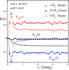
Figure 2: The energies of the exciton, phonon, and exciton-phonon interaction, i.e., $E_{\rm ex}(t),E_{\rm ph}(t)$ and $E_{\rm diag}(t)$, are displayed as a function of the time $t$ for the weak coupling case of $J=0.1,g=0.1,W=0.5$ and $\phi=0$. The open circles, solid triangles and solid line correspond to the results obtained with the single $\rm D_{2}$, ${\rm D}_{2}^{M=32}$ and ${\rm D}_{1}^{M=5}$ Ansätze, respectively.

Optical spectroscopy is another important aspect for the investigation of the polaron dynamics, as it provides valuable information on various correlation functions. First of all, the linear absorption spectra $F(\omega)$ calculated from the polaron dynamics on the basis of different Ansätze will be comprehensively studied. The autocorrelation function $F(t)$ of the exciton-phonon system is introduced

$$F(t) = {}_{\rm ph}\langle 0|_{\rm ex}\langle 0|e^{i\hat{H}t}\hat{P}e^{-i\hat{H}t}\hat{P}^{\dagger}|0\rangle_{\rm ex}|0\rangle_{\rm ph}$$ (17)

$$= {}_{\rm ph}\langle 0|_{\rm ex}\langle 0|\hat{P}e^{-i\hat{H}t}\hat{P}^{\dagger}|0\rangle_{\rm ex}|0\rangle_{\rm ph},$$

with the polarization operator

$$\hat{P}=\mu\sum_{n}(\hat{a}_{n}^{{\dagger}}|0\rangle_{\rm ex}\leavevmode\nobreak\ {}_{\rm ex}\langle 0|+|0\rangle_{\rm ex}\leavevmode\nobreak\ {}_{\rm ex}\langle 0|\hat{a}_{n}).$$ (18)

The linear absorption $F(\omega)$ is then calculated by means of the Fourier transformation,

$$F(\omega)=\frac{1}{\pi}{\rm Re}\int_{0}^{\infty}F(t)e^{i\omega t}dt.$$ (19)

In addition to the information provided by the linear absorption spectra, $2$D electronic spectra provide direct knowledge on exciton-exciton interactions and dephasing and relaxation processes that are elusive in the output from the traditional 1D spectroscopy. Theoretical simulation of 2D spectra involves the calculation of third order polarization $P(t)$, which can be expressed in terms of the nonlinear response function $R_{i}$, where $i$ goes from 1 to 4 Mukamel ; SunKeWei1 ; SunKeWei2 . The 2D electronic spectra are measured in two configurations that correspond to the rephasing (subscript R) and non-rephasing (subscript NR) contribution to the third order polarization $P(t)$, which, in the impulsive approximation, can be written as

$$P_{R}^{(3)}(t,T,\tau)\sim{-i}[R_{2}(t,T,\tau)+R_{3}(t,T,\tau)],$$

$$P_{NR}^{(3)}(t,T,\tau)\sim{-i}[R_{1}(t,T,\tau)+R_{4}(t,T,\tau)].$$ (20)

Where $\tau$ (the so-called coherence time) is the delay time between the first and second pulses, $T$ (the so-called population time) is the delay time between the second and third pulses, and $t$ is the delay time between the third pulse and measured signal. The rephasing and non-rephasing 2D spectra can be then obtained by performing two-dimensional Fourier-Laplace transformation of Eq. (II.2) as follows

$$S_{R}(\omega_{t},T,\omega_{\tau})=\mathrm{Re}\int_{0}^{\infty}\int_{0}^{\infty}dtd\tau{i}P_{R}^{(3)}(t,T,\tau)e^{-i\omega_{\tau}\tau+i\omega_{t}{t}},$$

$$S_{NR}(\omega_{t},T,\omega_{\tau})=\mathrm{Re}\int_{0}^{\infty}\int_{0}^{\infty}dtd\tau{i}P_{NR}^{(3)}(t,T,\tau)e^{i\omega_{\tau}\tau+i\omega_{t}{t}}.$$

The total $2$D signal is defined as the sum of the non-rephasing and the rephasing part

$$S(\omega_{t},T,\omega_{\tau})=S_{R}(\omega_{t},T,\omega_{\tau})+S_{NR}(\omega_{t},T,\omega_{\tau}).$$ (22)

In this work, we will apply the multiple ${\rm D}_{2}$ states to calculate the nonlinear response functions $R_{i}$ with special attention paid to the role of off-diagonal exciton-phonon coupling on the 2D spectra. The reader is referred to the Appendix D for more details on the applications of the multiple ${\rm D}_{2}$ Ansatze to the simulation of $2$D spectra.

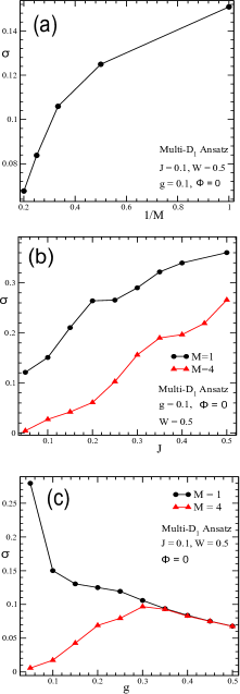
Figure 3: (a) The relative deviation $\sigma$ of the multi-${\rm D_{1}}$ Ansatz in a $16$-site molecular ring is displayed as a function of $1/M$ representing the inverse of the multiplicity. The set of parameters $J=0.1,g=1,W=0.5$ and $\phi=0$ is used. Moreover, the relative deviation $\sigma$ for the diagonal coupling case is also plotted as a function of the transfer integral $J$ in (b) and diagonal coupling strength $g$ in (c). In both of them, the lines with circles and triangles correspond to the results obtained at the multiplicity $M=1$ and $M=4$, respectively.

III Numerical results

III.1 Validity of variational dynamics

Figure 2 illustrates the time evolution of the system energies, including the exciton energy $E_{\rm ex}$, the phonon energy $E_{\rm ph}$ and the exciton-phonon interaction energy $E_{\rm diag}$, in a diagonal coupling only case with transfer integral $J=0.1$, band width $W=0.5$ and coupling strength $g=0.1$. For a molecular ring of $N=16$ sites, the energies obtained with three different Ansätze are compared (the open circles corresponding to the single $\rm D_{2}$ Ansatz, the solid triangles corresponding to the $\rm D_{2}^{M=32}$ Ansatz, and the solid line corresponding to the $\rm D_{1}^{M=5}$ Ansatz). Results obtained with the multi-$\rm D_{2}$ Ansatz with $M=32$ display obvious deviations from those by the single $\rm D_{2}$ Ansatz, demonstrating the improvement produced by the multiple Davydov trial states over its single Ansatz counterpart. In addition, the dynamics generated on the $\rm D_{1}$ trial state can be made more accurate by the $\rm D_{1}^{M=5}$ Ansatz, and results of $E_{\rm ex},E_{\rm ph}$ and $E_{\rm diag}$ by the $\rm D_{1}^{M=5}$ Ansatz are in perfect agreement with those obtained with the $\rm D_{2}^{M=32}$ Ansatz, which indicates the robustness of the polaron dynamics based on the multiple Davydov trial states when the multiplicity $M$ is sufficiently large.

A comprehensive test of the validity for our new trial states consisting of the multiple Davydov Ansätze is performed for various parameters sets $(J,W,g,\phi)$. In Fig. 3(a), the relative deviation $\sigma$, given by Eq. (14), is displayed as a function of $1/M$, for the diagonal coupling case of $J=0.1,W=0.5,g=0.1$ and $\phi=0$. As $M$ increases, the relative error $\sigma$ monotonically deceases, and the value $\sigma=0.067$ obtained at $1/M=0.2$ is very small, which indicates the length of the deviation vector $\vec{\delta}(t)$, as defined in Eqs. (12), is negligibly small with respect to those of the vectors $\vec{\chi}(t)$ and $\vec{\gamma}(t)$. Moreover, the result that the ${\rm D}_{1}^{M=5}$ Ansatz is comparable with $\sigma=0.033$ obtained with the ${\rm D}_{2}^{M=32}$ Ansatz demonstrates the accuracy of the multiple Davydov trial states when $M$ is sufficiently large.

In Fig. 3(b), the relative deviation $\sigma$ is displayed as a function of the transfer integral $J$ with circles and triangles corresponding to $M=1$ and $4$ of the multi-$\rm D_{1}$ Ansätze, respectively. Other parameters used in the simulation are $g=0.1,W=0.5$ and $\phi=0$. An obvious reduction in the relative error $\sigma$ has been found when the multiplicity $M$ is increased for the entire $J$ regime. Similarly, the relative error $\sigma$ against the diagonal coupling strength $g$ is displayed in Fig. 3(c) for $M=1$ and $4$, respectively. The relative error $\sigma$ is obviously reduced for the multiplicity $M=4$ in comparison with that of $M=1$ when $g<0.3$. However, these two curves overlap for $g>0.3$ as the exciton is self-trapped in one of the sites. The above results indicate that the multiple Davydov trial states will significantly improve the accuracy of the delocalized state, while in the localized state the single $\rm D_{1}$ Ansatz is sufficient. In addition, the multiple Davydov trial states in the off-diagonal coupling case are also investigated with the nonzero value of $\phi$. Taking the set of parameters $\phi=0.4$ and $g=J=W=0$ as an example, the relative error $\sigma$ is displayed as a function of $1/M$ in Fig. 4. As $M$ increases, the relative error $\sigma$ decreases, similar to the diagonal coupling case as shown in Fig. 3(a), although the value of $\sigma$ for $M=6$ ($\sigma=0.54$) remains somewhat large. For off-diagonal coupling, considerable improvements in accuracy can be achieved by utilizing multi-$\mathrm{D}_{2}$ with the increase of multiplicity M (see discussions in Ref. zhou_15 ).

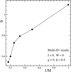
Figure 4: The relative deviation $\sigma$ from the multi-${\rm D}_{1}$ Ansatz is displayed as a function of $1/M$ for the the off-diagonal coupling case with the strength $\phi=0.4$, and other parameters $J=W=g=0$ are set.

III.2 Exciton probabilities and phonon displacements

Dynamical properties of the Holstein polaron, including the exciton probabilities and phonon displacements, are investigated by using the multiple Davydov trial states, in comparison with those obtained with the single Davydov Ansatz and the numerically exact HEOM method Tanimura1 ; Tanimura2 ; Tanimura3 ; Ishizaki (see Appendix B). Figure 5 illustrates the time evolution of the exciton probability $P_{\rm ex}(t,n)$ for the case of $J=0.5,W=0.5,g=0.1$ and $\phi=0$. For simplicity, a small ring with $N=10$ sites is used in the simulations. As depicted in Figs. 5(a) and 5(b), distinguishable deviation in $P_{\rm ex}(t,n)$ can be found between the variational results from the $\rm D^{M=1}_{1}$ and $\rm D^{M=8}_{1}$ Ansätze. Interestingly, the exciton probability $P_{\rm ex}(t,n)$ obtained from the HEOM method in Fig. 5(c) almost overlaps with that in Fig. 5(b) by the $\rm D_{1}^{M=8}$ Ansatz. Furthermore, the exciton probability difference between the variational method and the HEOM method, $\Delta P_{\rm ex}(t,n)$, as depicted in Fig. 5(d), is two order of magnitude smaller than the value of $P_{\rm ex}(t,n)$. It indicates that the variational dynamics of the Holstein polaron can be numerically exact if the multiplicity $M$ of the $\rm D_{1}$ Ansatz is sufficiently large. In Fig. 6, the exciton probabilities $P_{\rm ex}(t,n)$ at the site $n=5$ and $10$ are plotted in the top and the bottom panels with the solid line, the dashed line and the circles, corresponding to the variational results obtained with the single $\rm D_{1}$ and $\rm D_{1}^{M=8}$ Ansätze and the HEOM results, respectively. The near overlap of the dashed line and the circles further reconfirms the validity of the multi-$\rm D_{1}$ Ansatz.

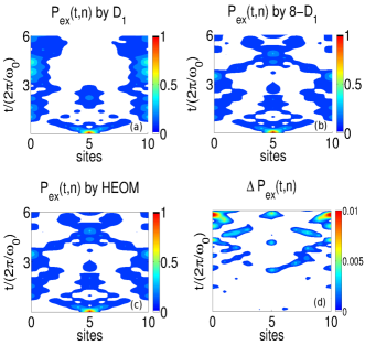
Figure 5: Time evolution of the exciton probability $P_{\rm ex}(t,n)$ for the case of $J=0.5,W=0.5,g=0.1$ and $\phi=0$ is displayed in (a), (b) and (c), corresponding to the results obtained with the single $\rm D_{1}$ Ansatz, the $\rm D_{1}^{M=8}$ Ansatz and the HEOM method, respectively. The difference $\Delta P_{\rm ex}(t,n)$ between the HEOM and the $\rm D_{1}^{M=8}$ variational method is also displayed in (d). For simplify, we set the size of the molecular ring $N=10$ in simulations.

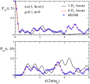
Figure 6: Time evolution of the exciton probability $P_{\rm ex}(t,n)$ with $n=5$ and $10$ are displayed in the top and bottom panel for the case of $J=0.5,W=0.5,g=0.1$ and $\phi=0$. In each panel, the solid line, dashed line and circles correspond to the variational results obtained with the single $\rm D_{1}$ and $\rm D_{1}^{M=8}$ Ansätze and the HEOM results, respectively. The size of the molecular ring is set to $N=10$.

Displayed in Figs. 7(a) and 7(c) are the exciton probability $P_{\rm ex}(t,n)$ and the phonon displacement $X_{\rm ph}(t,n)$ obtained with the single $\rm D_{1}$ Ansatz, respectively, for the case of $W=0.5,g=0.1,J=0.5$ and $\phi=0$. For comparsion, corresponding results of $P_{\rm ex}(t,n)$ and $X_{\rm ph}(t,n)$ obtained by the multi-$\rm D_{1}$ Ansatz with $M=4$ are presented in Figs. 7(b) and 7(d), respectively. Quite obvious difference is found in the excitonic behavior for the two cases when $t/(2\pi/\omega_{0})>3$. To be specific, the exciton probability calculated by the single $\rm D_{1}$ Ansatz staggers around two sites in the ring before being eventually trapped near site 8 accompanied by a thickened phonon cloud [cf. Fig. 7(c)], while that obtained by the multi-$\rm D_{1}$ Ansatz with $M=4$ continues to propagate in two opposite directions. The former behavior is apparently an artifact as the combination of $J=0.5$ and $g=0.1$ places the system firmly in the large polaron regime, incompatible with any form of self-trapping at long times. This shows that the single $\rm D_{1}$ Ansatz is too simplistic to capture accurate polaron dynamics at long times, especially in the weak coupling regime.

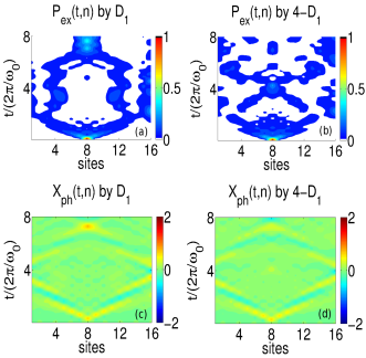
Figure 7: Time evolution of the exciton probability $P_{\rm ex}(t,n)$ and the phonon displacement $X_{\rm ph}(t,n)$ obtained with the single $\rm D_{1}$ Ansatz (left panel) and the ${\rm D}_{1}^{M=4}$ Ansatz (right panel) are displayed in (a)-(d) for the case of $W=0.5,g=0.1,J=0.5$ and $\phi=0$.

Next, we investigate the improvement on the polaron dynamics by the multi-$\rm D_{2}$ trial state. The exciton probability $P_{\rm ex}(t,n)$ calculated by the multi-$\rm D_{2}$ Ansatz with $M=16$ for two different sets of the parameters, ($J=0.1,g=0,\phi=0,W=0.5$) and ($J=0.1,g=0,\phi=0.1,W=0.5$), are displayed in Figs. 8(a) and 8(b), respectively. Corresponding $P_{\rm ex}(t,n)$ obtained by the single $\rm D_{2}$ Ansatz with the same two sets of parameters are shown in Figs. 8(c) and 8(d), which reveals a similar pattern of the exciton motion with the same speed of the exciton packet, $v=\omega_{0}/2\pi$, despite the jump of the off diagonal coupling strength from $0$ to $0.1$. In contrast, the exciton probability obtained with the multi-$\rm D_{2}$ Ansatz shows localization signatures at the off-diagonal coupling strength $\phi=0.1$, which is absent if $\phi=0$. It indicates that the combined effect of the transfer integral and the off-diagonal coupling will confine the exciton to the sites of the initial creation, despite that acting alone, either the transfer integral or the off-diagonal coupling may propagate the exciton wave packets. This phenomenon can be better understood after analyzing the energy band near the zone center where a discrete self-trapping transition occurs zhao_97 . Our calculations show that effective mass in the case of $\phi=0.1$ is larger than that of $\phi=0$, resulting in the polaron becoming less mobile. It demonstrates again that the polaron dynamics obtained with the multiple Davydov trial states is more accurate than that by the single Davydov trial state.

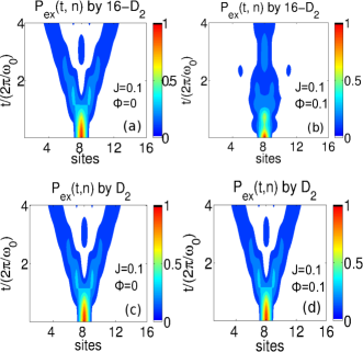
Figure 8: Time evolution of the exciton probability $P_{\rm ex}(t,n)$ is displayed for the case of $J=0.1$ and $\phi=0$ in the left panel and the case of $J=0.1$ and $\phi=0.1$ in the right panel. Other parameters used are $g=0,W=0.5$ and $N=16$ for both cases. Two different trial states, the ${\rm D}_{2}^{M=16}$ and ${\rm D}_{2}^{M=1}$ Ansätze, are used in the subfigures (a)-(b) and (c)-(d), respectively.

III.3 Absorption spectra

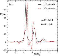
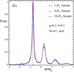
Figure 9: Linear absorption spectra $F(\omega)$ of a $16$-sites, one-dimensional ring of a coupled exciton-phonon system are displayed in (a) for the single $\rm D_{1}$ and $\rm D_{2}$ Ansätze and in (b) for the single $\rm D_{1}$, ${\rm D}_{1}^{M=4}$ and ${\rm D}_{2}^{M=16}$ Ansätze. The set of parameters $J=0.1,g=0.2,W=0.1$ and $\phi=0$ are used. A rescaled factor is adopted to normalize the spectral maxima to facilitate comparisons. The vertical dash-dotted line indicates the location of the zero-phonon line $\omega_{\rm m}/\omega_{0}=-0.75(1)$.

In this subsection we employ the multiple Davydov trial states to study the linear absorption spectra $F(\omega)$ defined in Eq. (19). To facilitate comparisons, spectral maxima are normalized to unity, and a damping factor of $0.08\omega_{0}$ is used luo_10 ; sun_10 . In Fig. 9, the linear absorption spectra $F(\omega)$ of a $16$-site ring is displayed for the case of $g=0.2,J=0.1,W=0.1$ and $\phi=0$. In the subfigure (a), we compare results obtained by the single $\rm D_{1}$ (solid) and single $\rm D_{2}$ (dashed) Ansätze. Large differences are found between these two curves, and negative values in the spectrum of the single $\rm D_{2}$ Ansatz point to its apparent invalidity. The multiple $\rm D_{1}$ trial states are capable to correct such inaccuracies in its single-$\rm D_{1}$ counterpart, as demonstrated in the subfigure (b) for a multiplicity of $4$. Similar corrections are also afforded by a multi-$\rm D_{2}$ Ansatz with a multiplicity of $16$, as shown in the same panel. Moreover, the position of the zero-phonon line, denoted by $\omega_{\rm m}$ with respect to $\omega_{0}$, is marked by the vertical dash-dotted line at $-0.75(1)$.

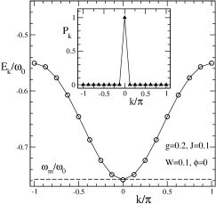
Figure 10: Polaron energy bands $E_{k}/\omega_{0}$ are calculated variationally using the Delocalized $\rm D_{1}$ Ansatz (solid line) and the Toyozawa Ansatz (open circles) for the case of $g=0.2,J=0.1,W=0.1$ and $\phi=0$. The position of zero-phonon line $\omega_{\rm m}/\omega_{0}$ is marked by the dashed line, consistent with the values of $E_{k=0}/\omega_{0}$. A lattice of $N=16$ sites is used in calculations. In the inset, the transition moment $P_{k}$ is plotted as a function of the crystal momentum $k$.

The zero-phonon line can be also determined by the ground-state polaron energy band $E_{k}$, where $k$ is the crystal momentum. In order to identify the relationship, the transition moment $P_{k}$ quantifying the transition probability between the vacuum state and the exciton state is introduced as $P_{k}=\left.{}_{\rm ex}\langle 0|_{\rm ph}\langle 0|\hat{P}^{\dagger}|\Psi_{k}\rangle\right.$, where $\hat{P}=\mu\sum_{n}(\hat{a}_{n}^{\dagger}|n\rangle_{\rm ex\leavevmode\nobreak\ ex}\langle n|+|n\rangle_{\rm ex\leavevmode\nobreak\ ex}\langle n|\hat{a}_{n})$ is the polarization operator, and $\Psi_{k}$ is the ground-state trial wave function with the crystal momentum $k$. By employing the variational method with the Toyozawa and Delocalized $\rm D_{1}$ Ansätze (details are shown in Appendix C), the ground-state wave function $\Psi_{k}$ can be obtained, and corresponding polaron energy band $E_{k}=\langle\Psi_{k}|\hat{H}|\Psi_{k}\rangle$ calculated. Variations carried out for different $k$ values are independent of each other, and the set of $E_{k}$ constitutes a variational estimate (an upper bound) for the polaron energy band. In Fig. 10, polaron energy bands $E_{k}/\omega_{0}$ calculated variationally for the case of $g=0.2,\leavevmode\nobreak\ \phi=0,\leavevmode\nobreak\ J=0.1$ and $W=0.1$, are plotted as a function of the crystal momentum $k/\pi$ with the solid and open circles, corresponding to the Delocalized $\rm D_{1}$ and Toyozawa Ansätze, respectively. For simplicity, we set $\mu=\omega_{0}=1$. Interestingly, the normalized position of the zero-phonon line, $\omega_{\rm m}/\omega_{0}$ in Fig. 9(b), is consistent with the value of $E_{k=0}/\omega_{0}$. It indicates that $\Psi_{k=0}$ is the bright state responsible for the zero-phonon line, in perfect agreement with the obtained transition probability $P_{k}$, which is nonzero only at the crystal momentum $k=0$ as depicted in the inset.

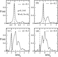
Figure 11: Linear absorption spectra $F(\omega)$ obtained with the $\rm D_{2}^{M=16}$ Ansatz are displayed in (a)-(d) for the off-diagonal coupling cases with the nonzero coupling strengths $\phi=0.1,0.2,0.3$ and $0.4$, respectively. Other parameters $g=W=J=0$ and $N=16$ are set. The vertical dash-dotted lines indicate locations of zero-phonon lines.

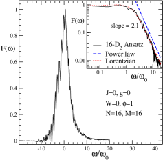
Figure 12: Linear absorption spectrum $F(\omega)$ of the $\rm D_{2}^{M=16}$ Ansatz is displayed for the off-diagonal coupling case with $\phi=1$. In the inset, the power-law and Lorenz fittings are given in the log-log scale with the dashed and dotted lines, respectively.

Moreover, absorption spectra in the presence of off-diagonal coupling ($\phi\neq 0$) are investigated with the aid of a multi-$\rm D_{2}$ Ansatz with $M=16$ (we set $J=g=W=0$ for simplicity). As shown in Fig. 11, with an increase in the off-diagonal coupling strength $\phi$, phonon sidebands of the linear absorption spectra become broadened and the intensity of the zero-phonon line is reduced. Vertical dashed lines shown in the $4$ panels of Fig. 11 denote the positions of the zero-phonon lines ($\omega_{\rm m}/\omega_{0}=-0.08,0.369,-0.956$ and $-1.93$). For strong off-diagonal coupling, such as the case of $\phi=1$, the linear absorption spectra, shown in Fig. 12, behave quite differently from those in weak off-diagonal coupling cases, such as $\phi=0.1$ and $0.2$ (cf. Fig. 11). All of the sharp peaks are smeared out, and the zero-phonon line almost disappears. In order to better understand the line shape, we plot the absorption spectrum in a log-log scale in the inset. A power-law fitting (dashed line) yields a slope of $2.1(1)$ indicating that the phonon sideband deviates from the Gaussian line shape. A Lorentzian line-shape function (dotted line) is then introduced for the fitting, consistent with the absorption spectrum obtained from the variational method.

III.4 2D spectra

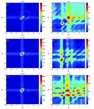
Figure 13: 2D spectra of the molecular ring for off-diagonal coupling strengths $\phi=0.1$ (left column) and $\phi=0.4$ (right column). Upper, middle and lower panels correspond to the population time $T=0,20,40$, respectively. Other parameters $g=W=J=0$ and $N=10$ are set.

In addition to the linear absorption spectra, fast and accurate implementation of the multidimensional spectroscopy is possible via the time-dependent variational method developed here. As an example, we present in this subsection $2$D spectra calculated for a molecular ring of $10$ sites using the multiple ${\rm D}_{2}$ Ansatz. For the secondary bath whose spectral density is defined by Eq. (53), we adopt the overdamped Brownian oscillator model with the Drude-Lorentz type spectral density

$$D(\omega)=2\eta\frac{\gamma\omega}{{\omega}^{2}+{\gamma}^{2}}$$ (23)

The resulting lineshape function [cf. Eq. (58)] can be evaluated analytically Mukamel ,

$$g(t) = \frac{\eta}{\gamma}\coth\frac{\gamma\beta}{2}[e^{-\gamma{t}}+\gamma{t}-1]-i\frac{\eta}{\gamma}[e^{-\gamma{t}}+\gamma{t}-1]$$ (24)

$$+\frac{4\eta\gamma}{\beta}\sum_{n=1}^{\infty}\frac{e^{-\nu_{n}t}+\nu_{n}t-1}{\nu_{n}(\nu_{n}^{2}-{\gamma}^{2})},$$

where $\nu_{n}=2\pi{n}/\beta$ is the Matsubara frequency. In our calculations, we set $\eta=0.1,\beta=5$ and $\gamma=0.02$.

In Fig. 13, $2$D spectra of the $10$-site ring are displayed for the case of $\phi=0.1$ (left panel) and $\phi=0.4$ (right panel). For simplicity, we set $J=g=W=0$, and adopt the toy model of J-aggregates with the tangential (head-to-tail) orientations of the transition dipoles. We first consider weak off-diagonal coupling. The $2$D spectra are shown in Figs. 13(a),(b), and (c) corresponding to the population time $T=0,20,40$, respectively. At $T=0$, the signal exhibits a single peak located at $(\omega_{\tau},\omega_{t})=(-0.08,-0.08)$, which is elongated along the diagonal line. As the population time increases, the elongation becomes less pronounced, and the peak appears more rounded. We then study the case of strong off-diagonal coupling with $\phi=0.4$, as depicted in the right panel of Fig. 13 for several values of the population time (see Figs. 13(d), (e) and (f) for $T=0,20$, and 40, respectively). Overall, it is found that strong exciton phonon coupling induces a pronounced vibronic multi-peak structure in the 2D spectra. With increasing population time, the shapes as well as the strengths for the peaks change, and we also find population cascades from high to low energy regions with lower $\omega_{t}$ for larger values of $T$, as demonstrated in Figs. 13(d), (e), and (f).

IV Conclusions

In this work, we have studied the dynamical properties of the Holstein polaron in a one-dimensional molecular ring using the Dirac-Frenkel time-dependent variational principle and an extended form of the Davydov trial states, also known as the “multi-D₁ Ansatz” (“multi-D₂ Ansatz”), which is a linear combination of the usual (single) Davydov $\rm D_{1}$ ($\rm D_{2}$) trial states. For both diagonal and off-diagonal exciton-phonon coupling, the relative error quantifying how closely the trial state follows the Schrödinger equation is found to decrease with the multiplicity $M$, reflecting the improvement in accuracy of the multiple Davydov trial states. Moreover, exciton probabilities calculated by the multiple Davydov trial states are obtained, in perfect agreement with those from a numerically exact approach employing the hierarchy equations of motion, demonstrating the great promise the multiple Davydov trial states hold as an efficient, robust description of dynamics of the complex quantum systems.

An abnormal self-trapping phenomenon is uncovered in the dynamical behavior of polaron with the increase of the off-diagonal coupling. Besides, the optical spectrum is also studied as a sensitive indicator of the accuracy of the variational polaron dynamics. Among our findings, linear absorption spectra from the multi-$\rm D_{1}$ Ansatz with a multiplicity of $4$ can be reproduced by the multi-$\rm D_{2}$ Ansatz with a multiplicity of $16$, and the positions of the zero-phonon lines are in good agreement with ground-state energy bands calculated by the Toyozawa and the Delocalized D₁ Ansätze in the weak coupling (transfer integral) regime. Moreover, for the first time, $2$D spectra have been calculated for systems with off-diagonal exciton-phonon coupling by employing the multiple ${\rm D}_{2}$ Ansatz to compute the nonlinear response function, testifying to the great potential of the multiple ${\rm D}_{2}$ Ansatz for fast, accurate implementation of multidimensional spectroscopy. It is also found that the signal exhibits a single peak for weak off-diagonal coupling, while a vibronic multi-peak structure appears for strong off-diagonal coupling.

Appendix A The Multi-${\rm D}_{1}$ trial state

The individual energy terms can be respectively calculated as follows

$$\left\langle{\rm D}^{M}_{1}\left(t\right)\right|H_{ex}\left|{\rm D}^{M}_{1}\left(t\right)\right\rangle$$

$$=-J\sum_{i,j}^{M}\sum_{n}\psi_{j,n}^{*}\left(t\right)\left[\psi_{i,n+1}\left(t\right)S_{j,n;i,n+1}\right.$$

$$\left.+\psi_{i,n-1}\left(t\right)S_{j,n;i,n-1}\right],$$

(25)

$$\left\langle{\rm D}^{M}_{1}\left(t\right)\right|H_{ph}\left|{\rm D}^{M}_{1}\left(t\right)\right\rangle$$

$$=\sum_{i,j}^{M}\sum_{n}\psi_{jn}^{\ast}\psi_{in}\sum_{q}\omega_{q}\lambda_{jnq}^{\ast}\lambda_{inq}S_{ji},$$

(26)

$$\left\langle{\rm D}^{M}_{1}\left(t\right)\right|H_{ex-ph}^{diag}\left|{\rm D}^{M}_{1}\left(t\right)\right\rangle$$

$$=-g\sum_{i,j}^{M}\sum_{n}\psi_{jn}^{\ast}\psi_{in}\sum_{q}\omega_{q}\left(e^{iqn}\lambda_{inq}+e^{-iqn}\lambda_{jnq}^{\ast}\right)S_{ji},$$

(27)

$$\left\langle{\rm D}^{M}_{1}\left(t\right)\right|H_{ex-ph}^{o.d.}\left|{\rm D}^{M}_{1}\left(t\right)\right\rangle$$

$$=\frac{1}{2}\phi\sum_{n,q}\sum_{i,j}^{M}\omega_{q}S_{j,n;i,n+1}\psi_{j,n}^{*}\left(t\right)\psi_{i,n+1}\left(t\right)$$

$$\left[e^{iqn}\left(e^{iq}-1\right)\lambda_{i,n+1,q}\left(t\right)+e^{-iqn}\left(e^{-iq}-1\right)\lambda_{jnq}^{*}\left(t\right)\right]$$

$$+\frac{1}{2}\phi\sum_{n,q}\sum_{i,j}^{M}\omega_{q}S_{j,n;i,n-1}\psi_{j,n}^{*}\left(t\right)\psi_{i,n-1}\left(t\right)$$

$$\left[e^{iqn}\left(1-e^{-iq}\right)\lambda_{i,n-1,q}\left(t\right)+e^{-iqn}\left(1-e^{iq}\right)\lambda_{jnq}^{*}\right],$$

where the Debye-Waller factor is formulated as

$$S_{ij} = \left\langle\lambda_{i}|\lambda_{j}\right\rangle,$$

$$S_{j,n;i,n+1} = \left\langle\lambda_{j,n}|\lambda_{i,n+1}\right\rangle,$$ (29)

The Dirac-Frenkel variational principle leads to equations of motion:

$$-i\sum_{i}^{M}\dot{\psi}_{in}S_{ki}$$

$$-\frac{i}{2}\sum_{i}^{M}\psi_{in}\sum_{q}\left(2\lambda_{knq}^{\ast}\dot{\lambda}_{inq}-\dot{\lambda}_{inq}\lambda_{inq}^{\ast}-\lambda_{inq}\dot{\lambda}_{inq}^{\ast}\right)S_{k,i}$$

$$=J\sum_{i}^{M}\left(\psi_{i,n+1}S_{k,n;i,n+1}+\psi_{i,n-1}S_{k,n;i,n-1}\right)$$

$$-\sum_{i}^{M}\psi_{in}\sum_{q}\omega_{q}\lambda_{knq}^{\ast}\lambda_{inq}S_{ki}$$

$$+g\sum_{i}^{M}\psi_{in}\sum_{q}\omega_{q}\left(e^{iqn}\lambda_{inq}+e^{-iqn}\lambda_{knq}^{\ast}\right)S_{ki}$$

$$-\frac{1}{2}\phi\sum_{i}^{M}\sum_{q}\omega_{q}\psi_{i,n+1}\left(t\right)\left[e^{iqn}\left(e^{iq}-1\right)\lambda_{i,n+1,q}\left(t\right)\right.$$

$$\left.+e^{-iqn}\left(e^{-iq}-1\right)\lambda_{knq}^{*}\left(t\right)\right]S_{k,n;i,n+1}$$

$$-\frac{1}{2}\phi\sum_{i}^{M}\sum_{q}\omega_{q}\psi_{i,n-1}\left(t\right)\left[e^{iqn}\left(1-e^{-iq}\right)\lambda_{i,n-1,q}\left(t\right)\right.$$

$$\left.+e^{-iqn}\left(1-e^{iq}\right)\lambda_{knq}^{*}\right]S_{k,n;i,n-1};$$ (30)

$$-i\sum_{i}^{M}\psi_{kn}^{\ast}\dot{\psi}_{in}\lambda_{inq}S_{ki}$$

$$-i\sum_{i}^{M}\psi_{kn}^{\ast}\psi_{in}\dot{\lambda}_{inq}S_{ki}$$

$$-\frac{i}{2}\sum_{i}^{M}\psi_{kn}^{\ast}\psi_{in}\lambda_{inq}S_{k,i}$$

$$\sum_{p}\left(2\lambda_{knp}^{\ast}\dot{\lambda}_{inp}-\dot{\lambda}_{inp}\lambda_{inp}^{\ast}-\lambda_{inp}\dot{\lambda}_{inp}^{\ast}\right)$$

$$=J\sum_{i}^{M}\psi_{k,n}^{*}\left(\psi_{i,n+1}\lambda_{i,n+1,q}S_{k,n;i,n+1}\right.$$

$$\left.+\psi_{i,n-1}\lambda_{i,n-1,q}S_{k,n;i,n-1}\right)$$

$$-\sum_{i}^{M}\psi_{kn}^{\ast}\psi_{in}\lambda_{inq}S_{ki}\left(\omega_{q}+\sum_{p}\omega_{p}\lambda_{knp}^{\ast}\lambda_{inp}\right)$$

$$+g\sum_{i}^{M}\psi_{kn}^{\ast}\psi_{in}\omega_{q}e^{-iqn}S_{ki}$$

$$+g\sum_{i}^{M}\psi_{kn}^{\ast}\psi_{in}\lambda_{inq}\sum_{p}\omega_{p}\left(e^{ipn}\lambda_{inp}+e^{-ipn}\lambda_{knp}^{\ast}\right)S_{k,i}$$

$$-\frac{1}{2}\phi\sum_{i}^{M}\omega_{q}\psi_{kn}^{*}\left[\psi_{i,n+1}e^{-iqn}\left(e^{-iq}-1\right)S_{k,n;i,n+1}\right.$$

$$\left.+\psi_{i,n-1}e^{-iqn}\left(1-e^{iq}\right)S_{k,n;i,n-1}\right]$$

$$-\frac{1}{2}\phi\sum_{p}\sum_{i}^{M}\omega_{p}\psi_{k,n}^{*}\psi_{i,n+1}\left[e^{ipn}\left(e^{ip}-1\right)\lambda_{i,n+1,p}\right.$$

$$\left.+e^{-ipn}\left(e^{-ip}-1\right)\lambda_{knp}^{*}\right]\lambda_{i,n+1,q}S_{k,n;i,n+1}$$

$$-\frac{1}{2}\phi\sum_{p}\sum_{i}^{M}\omega_{p}\psi_{k,n}^{*}\psi_{i,n-1}\left[e^{ipn}\left(1-e^{-ip}\right)\lambda_{i,n-1,p}\right.$$

$$\left.+e^{-ipn}\left(1-e^{ip}\right)\lambda_{knp}^{*}\right]\lambda_{i,n-1,q}S_{k,n;i,n-1}.$$ (31)

Appendix B Hierarchy equation of motion

For the Holstein model [Eq. (1)], let us denote $|n\rangle=\hat{a}_{n}^{\dagger}|0\rangle_{\mathrm{ex}}$ where $|0\rangle_{\mathrm{ex}}$ stands for the exciton vacuum. Then the reduced density matrix element for the exciton system is expressed in the path integral form with the factorized initial condition as LP_HEOM

$$\rho(n,n^{\prime};t)=$$ (32)

$$\int\mathcal{D}n\int\mathcal{D}n^{\prime}\rho(n_{0},n_{0}^{{}^{\prime}};t_{0})\times{e^{iS[n;t]}}F(n,n^{\prime};t)e^{-iS[n^{\prime};t]},$$

where $S[n]$ is an action of the exciton system, and $F[n,n^{\prime}]$ is the Feynman-Vernon influence functional

$$F[n,n^{\prime}]$$

$$=\exp(-\sum_{q}\omega_{q}^{2}\int_{t_{0}}^{t}ds\int_{t_{0}}^{s}ds^{\prime}{V_{q}^{*}}^{\times}(s)$$

$$\times[{V_{q}}^{\times}(s^{\prime})\coth(\beta\omega_{q}/2)\cos(\omega_{q}(s-s^{\prime}))$$

$$-i{V_{q}}^{\circ}(s^{\prime})\sin(\omega_{q}(s-s^{\prime}))]).$$ (33)

In the above equation, $\beta$ is the inverse of temperature ($\beta=1/k_{B}T$), and the abbreviations

$${V_{q}}^{\times}=V_{q}(n)-V_{q}(n^{\prime})\quad\quad{V_{q}}^{\circ}=V_{q}(n)+V_{q}(n^{\prime}),$$ (34)

are introduced with $\hat{V}_{q}^{\dagger}=g\sum_{n}\hat{a}_{n}^{\dagger}\hat{a}_{n}e^{iqn}$.

Equation (B) can be rewritten as

$$F[n,n^{\prime}]$$

$$=\exp(-\sum_{q}\omega_{q}^{2}\int_{t_{0}}^{t}ds\int_{t_{0}}^{s}ds^{\prime}{V_{q}^{*}}^{\times}(s)$$ (35)

$$\times[\frac{e^{i\omega_{q}(s-s^{\prime})}}{2}({V_{q}}^{\times}(s^{\prime})\coth{(\beta\omega_{q}/2)}-{V_{q}}^{\circ}(s^{\prime}))$$

$$+\frac{e^{-i\omega_{q}(s-s^{\prime})}}{2}({V_{q}}^{\times}(s^{\prime})\coth(\beta\omega_{q}/2)+{V_{q}}^{\circ}(s^{\prime}))]),$$

Taking derivative of Eq.(32), one has

$$\frac{\partial}{\partial{t}}\rho(n,n^{\prime};t)$$

$$=-i\mathcal{L}\rho(n,n^{\prime};t)$$ (36)

$$-\sum_{q}\omega_{q}^{2}{V_{q}^{*}}^{\times}(t)\int\mathcal{D}n\int\mathcal{D}n^{\prime}\rho(n_{0},n_{0}^{{}^{\prime}};t_{0})$$

$$\int_{0}^{t}ds^{\prime}[\frac{e^{i\omega_{q}(t-s^{\prime})}}{2}({V_{q}}^{\times}(s^{\prime})\coth(\beta\omega_{q}/2)-{V_{q}}^{\circ}(s^{\prime}))$$

$$+\frac{e^{-i\omega_{q}(t-s^{\prime})}}{2}({V_{q}}^{\times}(s^{\prime})\coth(\beta\omega_{q}/2)+{V_{q}}^{\circ}(s^{\prime}))]$$

$$\times{e^{iS[n,t]}}F(n,n^{\prime};t)e^{-iS[n^{\prime},t]},$$

If we use the following super-operator

$$\hat{\Phi}_{q}(t) = \omega_{q}^{2}{V_{q}^{*}}^{\times}(t)/2,$$

$$\hat{\Theta}_{q\pm}(t) = {V_{q}}^{\times}(t)\coth(\beta\omega_{q}/2)\mp{V_{q}}^{\circ}(t),$$ (37)

Eqs.(B) and (B) then can be simplified as

$$F[n,n^{\prime}]$$

$$=\exp(-\sum_{q}\int_{t_{0}}^{t}ds\int_{t_{0}}^{s}ds^{\prime}\Phi_{q}(s)\times[e^{i\omega_{q}(s-s^{\prime})}\Theta_{q+}(s^{\prime})$$

$$+e^{-i\omega_{q}(s-s^{\prime})}\Theta_{q-}(s^{\prime})]),$$ (38)

$$\frac{\partial}{\partial{t}}\rho(n,n^{\prime};t)$$

$$=-i\mathcal{L}\rho(n,n^{\prime};t)$$

$$-\sum_{q}\Phi_{q}(t)\int\mathcal{D}n\int\mathcal{D}n^{\prime}\rho(n_{0},n_{0}^{{}^{\prime}};t_{0})$$ (39)

$$\int_{0}^{t}ds^{\prime}[e^{i\omega_{q}(t-s^{\prime})}\Theta_{q+}(s^{\prime})$$

$$+e^{-i\omega_{q}(t-s^{\prime})}\Theta_{q-}(s^{\prime})]\times{e^{iS[n,t]}}F(n,n^{\prime};t)e^{-iS[n^{\prime},t]},$$

In order to derive the equations of motion, we introduce the auxiliary operator $\rho_{m_{1\pm},m_{2\pm},\cdots,m_{N\pm}}(n,n^{\prime};t)$ by its matrix element as

$$\rho_{m_{1\pm},m_{2\pm},\cdots,m_{N\pm}}(n,n^{\prime};t)=$$ (40)

$$\int\mathcal{D}n\int\mathcal{D}n^{\prime}\rho(n_{0},n_{0}^{{}^{\prime}};t_{0})\prod_{q=1}^{N}(\int_{t_{0}}^{t}dse^{i\omega_{q}(t-s)}\Theta_{q+}(s))^{m_{q+}}$$

$$(\int_{t_{0}}^{t}dse^{-i\omega_{q}(t-s)}\Theta_{q-}(s))^{m_{q-}}\times{e^{iS[n,t]}}F(n,n^{\prime})e^{-iS[n^{\prime},t]},$$

for non-negative integers $m_{1\pm},m_{2\pm},...,m_{N\pm}$. Note that only $\hat{\rho}_{0......0}(t)=\hat{\rho}(t)$ has a physical meaning and the others are introduced for computational purposes only. Differentiating $\rho_{m_{1\pm},m_{2\pm},...,m_{N\pm}}(n,n^{\prime};t)$ with respect to $t$, we can obtain the following hierarchy of equations in the operator form

$$\frac{\partial}{\partial{t}}\hat{\rho}_{m_{1\pm},\cdots,m_{N\pm}}(t)$$

$$=-i\mathcal{L}\hat{\rho}_{m_{1\pm},\cdots,m_{N\pm}}(t)$$

$$-i\sum_{q}\omega_{q}(m_{q-}-m_{q+})\hat{\rho}_{m_{1\pm},\cdots,m_{N\pm}}(t)$$

$$-\sum_{q}\hat{\Phi}_{q}(\hat{\rho}_{m_{1\pm},\cdots,m_{q+}+1,m_{q-},\cdots,m_{N\pm}}(t)$$

$$+\hat{\rho}_{m_{1\pm},\cdots,m_{q+},m_{q-}+1,\cdots,m_{N\pm}}(t))$$

$$+\sum_{q}(m_{q+}\hat{\Theta}_{q+}\hat{\rho}_{m_{1\pm},\cdots,m_{q+}-1,m_{q-},\cdots,m_{N\pm}}(t)$$

$$+m_{q-}\hat{\Theta}_{q-}\hat{\rho}_{m_{1\pm},\cdots,m_{q+},m_{q-}-1,\cdots,m_{N\pm}}(t)),$$ (41)

The HEOM consists of an infinite number of equations, but they can be truncated using a number of hierarchy elements. The infinite hierarchy of Eq.(B) can be truncated by the terminator as

$$\frac{\partial}{\partial{t}}\hat{\rho}_{m_{1\pm},\cdots,m_{N\pm}}(t)$$ (42)

$$=-(i\mathcal{L}+i\sum_{q}\omega_{q}(m_{q-}-m_{q+}))\times\hat{\rho}_{m_{1\pm},\cdots,m_{N\pm}}(t).$$

The total number of hierarchy elements can be evaluated as $L_{\mathrm{tot}}=(N_{\mathrm{trun}}+2N)!/N_{\mathrm{trun}}!(2N)!$, while the total number of termination elements is $L_{\mathrm{term}}=(N_{\mathrm{trun}}+2N-1)!/(2N-1)!N_{\mathrm{trun}}!$, where $N_{\mathrm{trun}}$ is the depth of the hierarchy for $m_{q\pm}(q=1,\cdots,N)$. In practice, we can set the termination elements to zero and thus the number of hierarchy elements for the calculation can be reduced as $L_{\mathrm{calc}}=L_{\mathrm{tot}}-L_{\mathrm{term}}$.

Appendix C The Delocalized D₁ Ansatz and the Toyozawa Ansatz

Our interest in this work includes the polaron ground-state energy band, computed as

$$E(\kappa)=\langle\Psi(\kappa)|\hat{H}|\Psi(\kappa)\rangle,$$ (43)

where$|\Psi(\kappa)\rangle$ is an appropriately normalized, delocalized trial state, and $\hat{H}$ is the system Hamiltonian. The joint crystal momentum is indicated by the Greek $\kappa$. It should be noted that the crystal momentum operator commutes with the system Hamiltonian, and energy eigenstates are also eigenfunctions of the crystal momentum. Therefore, variations for distinct $\kappa$ are independent. The set of $E(\kappa)$ constitutes a variational estimate (an upper bound) for the polaron energy band. The relaxation iteration technique, viewed as an efficient method for identifying energy minima of a complex variational system, is adopted in this work to obtain numerical solutions to a set of self-consistency equations derived from the variational principle. To achieve efficient and stable iterations toward the variational ground state, one may take advantage of the continuity of the ground state with respect to small changes in system parameters over most of the phase diagram and may initialize the iteration using a reliable ground state already determined at some nearby points in parameter space. Starting from those limits where exact solutions can be obtained analytically and executing a sequence of variations along well-chosen paths through the parameter space using solutions from one step to initialize the next, the whole parameter space can be explored.

As the D₁ and D₂ Ansätze are localized states from the soliton theory, but without considering a form factor of a delocalized state. The polaron state have been analyzed with the delocalized D₁ and Toyozawa Ansätze, both of which are Bloch states with the designated crystal momentum. The D₁ and D₂ Ansätze can be delocalized into the delocalized D₁ and Toyozawa Ansätze via a projection operator $\hat{P}_{\kappa}$

$$\hat{P}_{\kappa}=N^{-1}\underset{n}{\sum}e^{i(\kappa-\hat{P})n}=\delta(\kappa-\hat{P}),$$ (44)

where

$$\hat{P}=\underset{k}{\sum}ka_{k}^{\dagger}a_{k}+\underset{q}{\sum}qb_{q}^{\dagger}b_{q},$$ (45)

The delocalized D₁ Ansatz are then obtained after the delocalization onto the usual $\rm D_{1}$ Ansatz,

$$|\Psi_{1}(\kappa)\rangle=|\kappa\rangle\langle\kappa|\kappa\rangle^{-1/2},$$ (46)

$$|\kappa\rangle = \underset{n}{\sum}e^{i\kappa n}\underset{n1}{\sum}\alpha_{n_{1}-n}^{\kappa}a_{n_{1}}^{\dagger}$$

$$\exp[-\underset{n_{2}}{\sum}(\beta_{n_{1}-n,n_{2}-n}^{\kappa}b_{n_{2}}^{\dagger}-{\rm H.c.})]|0\rangle,$$

where $\rm H.c.$ stands for the Hermitian conjugate, $|0\rangle$ is the product of the exciton and phonon vacuum states, $\alpha_{n_{1}-n}^{\kappa}$ is the exciton amplitude, and the phonon displacement $\beta_{n_{1}-n,n_{2}-n}^{\kappa}$ depends on $n_{1}$ and $n_{2}$, respectively, the sites at which an electronic excitation and a phonon are generated.

After the delocalization onto the usual ${\rm D}_{2}$ Ansatz, the Toyozawa Ansatz is given by

$$|\Psi_{2}(\kappa^{\prime})\rangle=|\kappa^{\prime}\rangle\langle\kappa^{\prime}|\kappa^{\prime}\rangle^{-1/2},$$ (48)

$$|\kappa^{\prime}\rangle = \underset{n}{\sum}e^{i\kappa^{\prime}n}\underset{n1}{\sum}\psi_{n_{1}-n}^{\kappa^{\prime}}a_{n_{1}}^{\dagger}$$

$$\exp[-\underset{n2}{\sum}(\lambda_{n_{2}-n}^{\kappa^{\prime}}b_{n_{2}}^{\dagger}-{\rm H.c.})]|0\rangle,$$

where $\psi_{n_{1}-n}^{\kappa^{\prime}}$ is the exciton amplitude analogous to $\alpha_{n_{1}-n}^{\kappa}$ in the delocalized D₁ Ansatz, and $\lambda_{n_{2}-n}^{\kappa^{\prime}}$ is the phonon displacement. Actually, $\lambda_{n_{2}-n}^{\kappa^{\prime}}$ is just one column of the phonon displacement matrix $\beta_{n_{1}-n,n_{2}-n}^{\kappa}$ in the delocalized D₁ Ansatz.

Appendix D Simulation of 2D spectra using multiple D₂ Ansatze

In order to describe the population decays and dephasings induced by solvent, we add additional term $H_{B}+H_{SB}$ to the Hamiltonian (1)

$$\hat{H} = \hat{H}_{ex}+\hat{H}_{ph}+\hat{H}_{ex-ph}^{diag}+\hat{H}_{ex-ph}^{o.d.}+\hat{H}_{B}+\hat{H}_{SB}$$ (50)

$$= \hat{H}_{S}+\hat{H}_{B}+\hat{H}_{SB}$$

where we have included vibrational modes with significant exciton-phonon coupling into system Hamiltonian, i.e., $\hat{H}_{S}=\hat{H}_{ex}+\hat{H}_{ph}+\hat{H}_{ex-ph}^{diag}+\hat{H}_{ex-ph}^{o.d.}$, and treated the rest of vibrational modes as a heat bath. We assume a harmonic bath with site-independent and diagonal system bath coupling SunKeWei1 ; SunKeWei2 ; LP_OD

$$\hat{H}_{B} = \sum_{j}\hbar\Omega_{j}c_{j}^{\dagger}c_{j}$$ (51)

$$\hat{H}_{SB} = \sum_{j}\sum_{n=1}^{N}\kappa_{j}\hbar\Omega_{j}(c_{j}^{\dagger}+c_{j})a_{n}^{\dagger}a_{n}$$ (52)

Here, $c_{j}(c_{j}^{\dagger})$ is the annihilation (creation) operator of the $j$th bath mode with frequency $\Omega_{j}$, and $\kappa_{j}$ is the corresponding exciton-bath coupling strength. The bath spectral density is specified by

$$D(\omega)=\sum_{j}\kappa_{j}^{2}\Omega_{j}^{2}\delta(\omega-\Omega_{j})$$ (53)

It is noted that system-bath Hamiltonian $\hat{H}_{SB}$ commutes with the system Hamiltonian $\hat{H}_{S}$, and as a result, the nonlinear response function can be represented as a product of the system and bath. Furthermore, by making use of the fact that the system-bath coupling is the same for all excitons, the effect of bath can be taken into account through lineshape factors $F_{i}$ in the framework of second-order cummulant expansion. Finally, we arrived at the formulas for the nonlinear response function SunKeWei1

$$R_{1}{(t,T,\tau)} = F_{1}(t,T,\tau)\sum_{n,n^{\prime},n^{\prime\prime},n^{\prime\prime\prime}}C_{n,n^{\prime},n^{\prime\prime},n^{\prime\prime\prime}}$$

$${}_{ph}\langle{0}|\langle{n}|e^{iH_{S}T}|n^{\prime}\rangle\langle{n^{\prime\prime}}|e^{-H_{S}(t+T+\tau)}|n^{\prime\prime\prime}\rangle|0\rangle_{\rm ph}$$

$$R_{2}{(t,T,\tau)} = F_{2}(t,T,\tau)\sum_{n,n^{\prime},n^{\prime\prime},n^{\prime\prime\prime}}C_{n,n^{\prime},n^{\prime\prime},n^{\prime\prime\prime}}$$

$${}_{ph}\langle{0}|\langle{n}|e^{iH_{S}(\tau+T)}|n^{\prime}\rangle\langle{n^{\prime\prime}}|e^{-H_{S}(t+T)}|n^{\prime\prime\prime}\rangle|0\rangle_{\rm ph}$$

$$R_{3}{(t,T,\tau)} = F_{3}(t,T,\tau)\sum_{n,n^{\prime},n^{\prime\prime},n^{\prime\prime\prime}}C_{n,n^{\prime},n^{\prime\prime},n^{\prime\prime\prime}}$$

$${}_{ph}\langle{0}|\langle{n}|e^{iH_{S}\tau}|n^{\prime}\rangle\langle{n^{\prime\prime}}|e^{-H_{S}t}|n^{\prime\prime\prime}\rangle|0\rangle_{\rm ph}$$

$$R_{4}{(t,T,\tau)} = F_{4}(t,T,\tau)\sum_{n,n^{\prime},n^{\prime\prime},n^{\prime\prime\prime}}C_{n,n^{\prime},n^{\prime\prime},n^{\prime\prime\prime}}$$ (54)

$${}_{ph}\langle{0}|\langle{n}|e^{-iH_{S}t}|n^{\prime}\rangle\langle{n^{\prime\prime}}|e^{-H_{S}\tau}|n^{\prime\prime\prime}\rangle|0\rangle_{\rm ph}$$

Here

$$C_{n,n^{\prime},n^{\prime\prime},n^{\prime\prime\prime}}=(\bf{e_{1}}\boldsymbol{\mu_{n}})(\bf{e_{2}}\boldsymbol{\mu_{n^{\prime}}})(\bf{e_{3}}\boldsymbol{\mu_{n^{\prime\prime}}})(\bf{e_{4}}\boldsymbol{\mu_{n^{\prime\prime\prime}}})$$ (55)

are the geometrical factors which must be averaged over orientations of the transition dipole moments $\boldsymbol{\mu_{n}}$. For simplicity, we can assume all laser fields have the same polarization, then the averaging can be done analytically, leading to

$$C_{n,n^{\prime},n^{\prime\prime},n^{\prime\prime\prime}} = \frac{1}{15}((\boldsymbol{\mu}_{n}\boldsymbol{\mu}_{n^{\prime}})(\boldsymbol{\mu}_{n^{\prime\prime}}\boldsymbol{\mu}_{n^{\prime\prime\prime}})$$

$$+(\boldsymbol{\mu}_{n}\boldsymbol{\mu}_{n^{\prime\prime}})(\boldsymbol{\mu}_{n^{\prime}}\boldsymbol{\mu}_{n^{\prime\prime\prime}})+(\boldsymbol{\mu}_{n}\boldsymbol{\mu}_{n^{\prime\prime\prime}})(\boldsymbol{\mu}_{n^{\prime\prime}}\boldsymbol{\mu}_{n^{\prime}}))$$

The lineshape factors $F_{i}$ can be easily evaluated as Mukamel

$$F_{1}(t,T,\tau) = e^{-g^{*}(t)-g(\tau)-g^{*}(T)+g^{*}(T+t)+g(\tau+T)-g(\tau+T+t)}$$

$$F_{2}(t,T,\tau) = e^{-g^{*}(t)-g^{*}(\tau)+g(T)-g(T+t)-g^{*}(\tau+T)+g^{*}(\tau+T+t)}$$

$$F_{3}(t,T,\tau) = e^{-g(t)-g^{*}(\tau)+g^{*}(T)-g^{*}(T+t)-g^{*}(\tau+T)+g^{*}(\tau+T+t)}$$

$$F_{4}(t,T,\tau) = e^{-g(t)-g(\tau)-g(T)+g(T+t)+g(\tau+T)-g(\tau+T+t)}$$

where $g(t)$ is the lineshape function

$$g(t) = \int_{0}^{\infty}d\omega\frac{D(\omega)}{\omega^{2}}\times$$ (58)

$$\big{[}\coth\frac{\hbar\omega\beta}{2}(1-\cos{\omega{t}})+i(\sin{\omega{t}}-\omega{t})\big{]}$$

The next crucial step is to approximate the propagator in terms of multiple $D_{2}$ Ansatze, i.e,

$$e^{-iH_{s}t}|n\rangle|0\rangle_{ph}$$

$$=\sum_{i}^{M}\sum_{n}^{N}\psi_{i,n}\hat{a}_{n}^{\dagger}|0\rangle_{ex}\exp\left\{\sum_{q}\left[\lambda_{iq}\hat{b}_{q}^{\dagger}-\lambda_{iq}^{\ast}\hat{b}_{q}\right]\right\}\left|0\right\rangle_{\rm ph}$$

Explicitly, we have final expressions for the nonlinear response function

$$R_{1}{(t,T,\tau)} = F_{1}(t,T,\tau)\sum_{n,n^{\prime},n^{\prime\prime},n^{\prime\prime\prime}}C_{n,n^{\prime},n^{\prime\prime},n^{\prime\prime\prime}}\sum_{i,j=1}^{M}\psi_{jn^{\prime}}^{n*}(T)$$

$$\psi_{in^{\prime\prime}}^{n^{\prime\prime\prime}}(\tau+T+t)e^{-\frac{1}{2}\sum_{q}(|\lambda_{jq}^{n}(T)|^{2}+|\lambda_{iq}^{n^{\prime\prime\prime}}(\tau+T+t)|^{2})}$$

$$e^{\sum_{q}\lambda_{jq}^{n*}(T)\lambda_{iq}^{n^{\prime\prime\prime}}(\tau+T+t)e^{i\omega_{q}t}}$$

$$R_{2}{(t,T,\tau)} = F_{2}(t,T,\tau)\sum_{n,n^{\prime},n^{\prime\prime},n^{\prime\prime\prime}}C_{n,n^{\prime},n^{\prime\prime},n^{\prime\prime\prime}}\sum_{i,j=1}^{M}\psi_{jn^{\prime}}^{n*}(T+\tau)$$

$$\psi_{in^{\prime\prime}}^{n^{\prime\prime\prime}}(T+t)e^{-\frac{1}{2}\sum_{q}(|\lambda_{jq}^{n}(T+\tau)|^{2}+|\lambda_{iq}^{n^{\prime\prime\prime}}(T+t)|^{2})}$$

$$e^{\sum_{q}\lambda_{jq}^{n*}(T+\tau)\lambda_{iq}^{n^{\prime\prime\prime}}(T+t)e^{i\omega_{q}t}}$$

$$R_{3}{(t,T,\tau)} = F_{3}(t,T,\tau)\sum_{n,n^{\prime},n^{\prime\prime},n^{\prime\prime\prime}}C_{n,n^{\prime},n^{\prime\prime},n^{\prime\prime\prime}}\sum_{i,j=1}^{M}\psi_{jn^{\prime}}^{n*}(\tau)$$

$$\psi_{in^{\prime\prime}}^{n^{\prime\prime\prime}}(t)e^{-\frac{1}{2}\sum_{q}(|\lambda_{jq}^{n}(\tau)|^{2}+|\lambda_{iq}^{n^{\prime\prime\prime}}(t)|^{2})}$$

$$e^{\sum_{q}\lambda_{jq}^{n*}(\tau)\lambda_{iq}^{n^{\prime\prime\prime}}(t)e^{i\omega_{q}(t+T)}}$$

$$R_{4}{(t,T,\tau)} = F_{4}(t,T,\tau)\sum_{n,n^{\prime},n^{\prime\prime},n^{\prime\prime\prime}}C_{n,n^{\prime},n^{\prime\prime},n^{\prime\prime\prime}}\sum_{i,j=1}^{M}\psi_{jn^{\prime}}^{n*}(-t)$$ (60)

$$\psi_{in^{\prime\prime}}^{n^{\prime\prime\prime}}(\tau)e^{-\frac{1}{2}\sum_{q}(|\lambda_{jq}^{n}(-t)|^{2}+|\lambda_{iq}^{n^{\prime\prime\prime}}(\tau)|^{2})}$$

$$e^{\sum_{q}\lambda_{jq}^{n*}(-t)\lambda_{iq}^{n^{\prime\prime\prime}}(\tau)e^{-i\omega_{q}T}}$$

References

- (1) Z. An, C. Q. Wu, and X. Sun, Phys. Rev. Lett. 93, 216407 (2004).
- (2) B. Zheng, J. Wu, W. Sun, and C. Liu, Chem. Phys. Lett. 425, 123 (2006).
- (3) X. Liu, K. Gao, J. Fu, Y. Li, J. Wei, and S. Xie, Phys. Rev. B 74, 172301 (2006).
- (4) C. Bronner and P. Tegeder, Phys. Rev. B 89, 115105 (2014).
- (5) I. Timrov, T. Kampfrath, J. Faure, N. Vast, C. R. Ast, C. Frischkorn, M. Wolf, P. Gava, and L. Perfetti, Phys. Rev. B 85, 155139 (2012).
- (6) V. Chikan and D. F. Kelleya, J. Phys. Chem. 117, 8944 (2002).
- (7) V. I. Klimov, A. A. Mikhailovsky, D. W. McBranch, C. A. Leatherdale, and M. G. Bawendi, Phys. Rev. B 61, R13349 (2000).
- (8) S. H. Kim, R. H. Wolters, and J. R. Heath, J. Chem. Phys. 105, 7957 (1996).
- (9) K. Sauer, Annu. Rev. Phys. Chem. 30, 155 (1979).
- (10) T. Renger, V. May, and Oliver KüKhn, Phys. Rep. 343, 137 (2001).
- (11) R. E. Blankenship, Molecular Mechanisms of Photosynthesis (Blackwell Science, Oxford/Malden, 2002).
- (12) R. van Grondelle and V. I. Novoderezhkin, Phys. Chem. Chem. Phys. 8, 793 (2006).
- (13) L. P. Chen, P. Shenai, F. L. Zheng, A. Somoza, and Y. Zhao, Molecules. 20, 15224, (2015)
- (14) S. Tomimoto, H. Nansei, S. Saito, T. Suemoto, J. Takeda, and S. Kurita, Phys. Rev. Lett. 81, 417 (2000).
- (15) S. L. Dexheimer, A. D. Van Pelt, J. A. Brozik, and B. I. Swanson,Phys. Rev. Lett. 84, 4425 (2000).
- (16) A. Sugita, T. Saito, H. Kano, M. Yamashita, and T. Kobayashi, Phys. Rev. Lett. 86, 2158 (2001).
- (17) F. X. Morrissey and S. L. Dexheimer, Phys. Rev. B 81, 094302 (2010).
- (18) A. S. Alexandrov and Sir N. Mott, Polarons and Bipolarons (World Scientific, London, 1995).
- (19) F. M. Peeters and J. T. Devreese, Solid State Phys. 38, 81 (1984).
- (20) J. Ranninger, in Polarons in Bulk Materials and Systems with Reduced Dimensionality, edited by G. Iadonisi, J. Ranninger, and G. De Filippis, International School of Physics Enrico Fermi, (IOS Press, Amsterdam) 161, 1(2006)
- (21) T. Holstein, Ann. Phys. (N.Y.) 8, 325 (1959)
- (22) T. Holstein, Ann. Phys. (N.Y.) 8, 343 (1959).
- (23) W. P. Su, J. R. Schrieffer, and A. J. Heeger, Phys. Rev. Lett. 42, 1698 (1979).
- (24) L. A. Dissado and S. H. Walmsley, Chem. Phys. 86, 375 (1984).
- (25) H. Sumi, Chem. Phys. 130, 433 (1989).
- (26) Y. Zhao, D. W. Brown, and K. Lindenberg, J. Chem. Phys. 100, 2335 (1994).
- (27) D. M. Chen, J. Ye, H. J. Zhang, and Y. Zhao, J. Phys. Chem. B 115, 5312 (2011).
- (28) B. Luo, J. Ye, C. B. Guan and Y. Zhao, Phys. Chem. Chem. Phys. 12, 6045 (2010).
- (29) J. Sun, B. Luo, and Y. Zhao, Phys. Rev. B 82, 014305 (2010).
- (30) R. W. Munn and R. Silbey, J. Chem. Phys. 83, 1843(1985); 83, 1854 (1985).
- (31) Y. Zhao, Doctoral thesis, University of California, San Diego, (1994).
- (32) Y. Zhao, G. Q. Li, J. Sun, and W. H. Wang, J. Chem. Phys. 129, 124114 (2008).
- (33) Q. Liu, Y. Zhao, W. Wang, and T. Kato, Phys. Rev. B 79, 165105 (2009).
- (34) L. C. Ku, A. Trugman, Phys. Rev. B 75, 014307 (2007).
- (35) T. Meier, Y. Zhao, V. Chernyak, and S. Mukamel, J. Chem. Phys. 107, 3876 (1997).
- (36) Y. Zhao, D. W. Brown, and K. Lindenberg, J. Chem. Phys. 106, 2728 (1997).
- (37) Y. Zhao, D. W. Brown, and K. Lindenberg, J. Chem. Phys. 107, 3159 (1997); D. Brown, K. Lindenberg, and Y. Zhao, ibid. 107, 3179 (1997).
- (38) J. Sun, L. W. Duan, and Y. Zhao, J. Chem. Phys. 138, 174116 (2013).
- (39) N. J. Zhou, L.P. Chen, Y. Zhao, D. Mozyrsky, V. Chernyak, and Y. Zhao, Phys. Rev. B 90, 155135 (2014).
- (40) P. A. M. Dirac, Proc. Cambridge Philos. Soc. 26, 376 (1930); J. Frenkel, Wave Mechanics (Oxford University Press, 1934).
- (41) Y. Zhao, B. Luo, Y. Y. Zhang, and J. Ye, J. Chem. Phys. 137, 084113 (2012).
- (42) A. S. Davydov and N. I. Kislukha, Zh. Eksp. Teor. Fiz,. 71,1090 (1976) [Sov. Phys. JETP. 44, 571 (1976)]
- (43) A. S. Davydov, Solitons in Molecular Systems (Reidel, Dordrecht, 1985)
- (44) M. J. Škrinjar, D. V. Kapor and S. D. Stojanović , Phys. Rev. A 38, 6402 (1988), and references therein.
- (45) W. Förner, J. Phys.: Condens. Matter 5, 3897 (1993); Phys. Rev. B 53, 6291 (1996).
- (46) L. C. Hansson, Phys. Rev. Lett. 73, 2927 (1994).
- (47) N. J. Zhou, Z. K. Huang, J. F. Zhu, V. Chernyak, and Y. Zhao, J. Chem. Phys. 143, 014113 (2015).
- (48) T. Brixner, J. Stenger, H. M. Vaswani, M. Cho, R. E. Blankenship, G. R. Fleming, Nature 434, 625 (2005).
- (49) G. S. Engel, T. R. Calhoun, E. L. Read, T. K. Ahn, T. Mancal, Y. C. Chung, R. E. Blankenship, G. R. Fleming. Nature 446, 782 (2007).
- (50) E. Collini, C. Y. Wong, K. E. Wilk, P. M. G. Curmi, P. Brumer, G. D. Scholes. Nature, 463, 644 (2010).
- (51) G. Panitchayangkoon, D. Hayes, K. A. Fransted, J. R. Caram, E. Harel, J. Z. Wen, R. E. Blankenship, G. S. Engel. Proc. Natl. Acad. Sci. USA 107, 12766 (2010).
- (52) J. A. Myers, K. L. M. Lewis, F. D. Fuller, P. F. Tekavec, C. F. Yocum, J. P. Ogilvie. J. Phys. Chem. Lett, 1, 2774 (2010).
- (53) K. L. M. Lewis, J. P. Ogilvie. J. Phys. Chem. Lett, 3, 503 (2012)?
- (54) E. Romero, R. Augulis, V. I. Novoderezhkin, M. Ferretti, J. Thieme, D. Zigmantas, R. van Grondelle. Nat, Phys. 10,676 (2014)
- (55) S. Mukamel, Principles of Nonlinear Optical Spectroscopy (Oxford University Press, New York, 1995).
- (56) T. D. Huynh, K. W. Sun, M. F. Gelin, and Y. Zhao, J. Chem. Phys. 139, 104103 (2013).
- (57) K. W. Sun, M. F. Gelin, V. Y. Chernyak, and Y. Zhao, J. Chem. Phys. 142, 212448 (2015).
- (58) Y. Tanimura, R. Kubo, J. Phys. Soc. Jpn, 58, 101 (1989)
- (59) Y. Tanimura, Phys. Rev. A, 41, 6676 (1990).
- (60) Y. Tanimura, J. Phys. Soc. Jpn, 75, 082001 (2006).
- (61) A. Ishizaki, Y. Tanimura, J. Phys. Soc. Jpn, 74, 3131 (2005)
- (62) L. P. Chen, Y. Zhao, and Y. Tanimura, J. Phys. Chem. Lett. 6, 3110 (2015).
- (63) L. P. Chen, M. F. Gelin, W. Domcke, and Y. Zhao, J. Chem. Phys. 142, 164106 (2015).