Sparse Additive Gaussian Process Regression

Abstract

In this paper we introduce a novel model for Gaussian process (GP) regression in the fully Bayesian setting. Motivated by the ideas of sparsification, localization and Bayesian additive modeling, our model is built around a recursive partitioning (RP) scheme. Within each RP partition, a sparse GP (SGP) regression model is fitted. A Bayesian additive framework then combines multiple layers of partitioned SGPs, capturing both global trends and local refinements with efficient computations. The model addresses both the problem of efficiency in fitting a full Gaussian process regression model and the problem of prediction performance associated with a single SGP. Our approach mitigates the issue of pseudo-input selection and avoids the need for complex inter-block correlations in existing methods. The crucial trade-off becomes choosing between many simpler local model components or fewer complex global model components, which the practitioner can sensibly tune. Implementation is via a Metropolis-Hasting Markov chain Monte-Carlo algorithm with Bayesian back-fitting. We compare our model against popular alternatives on simulated and real datasets, and find the performance is competitive, while the fully Bayesian procedure enables the quantification of model uncertainties.

Keywords: Sparse Gaussian Process, Recursive Partition Scheme, Bayesian Additive Model, Nonparametric Regression.

1 Introduction

Gaussian process (GP) regression is a widely adopted regression model (Rasmussen and Williams, 2006). Taking a Bayesian approach, its posterior distribution provides a principled way to quantify uncertainties while having nice theoretical properties (Gelman et al., 2013). However, the computational cost of GP likelihood evaluations based on an observed dataset $\{y,\mathcal{X}\}$ of size $n$ is of order $\mathcal{O}(n^{3})$, which primarily results from the need to invert an $n\times n$ covariance matrix. Therefore, the computational cost could be prohibitively high in scenarios where large datasets need to be analyzed. It is a focus of much current research to solve this problem of high computational cost for GP regression (Banerjee et al., 2012; Liu et al., 2018).

Many approaches to circumvent this problem have been explored, such as low-rank covariance approximation (Titsias, 2009), model likelihood approximations (Kaufman et al., 2008) and local GP approximations (Snelson and Ghahramani, 2007; Gramacy and Apley, 2015). However, most of these approaches are not fully Bayesian.

We are inspired by the idea of low-rank sparse GP regression (Snelson and Ghahramani, 2006) and localization ideas (Chipman et al., 1998; Lee et al., 2017; Gramacy and Apley, 2015; Park and Huang, 2016; Nguyen-Tuong et al., 2009; Chipman et al., 2016; Lee et al., 2017), but we still want to incorporate these methods within a fully Bayesian framework. Borrowing the framework of Bayesian (generalized) additive modeling (Hastie and Tibshirani, 1990, 2000), we propose the Sparse Additive Gaussian Process (SAGP) model. SAGP combines sparse GP regression and a recursive partition (RP) scheme within a fully Bayesian model. It turns out that our approach can simultaneously handle both local and global features in large datasets while realizing gains in computational efficiency. Furthermore, it provides principled uncertainty quantification for parameters and posterior predictions. A key feature of the approach is a much simplified fixed partitioning scheme that avoids the added computational costs of stochastic tree-based partitioning models (e.g. (Chipman et al., 1998, 2016; Gramacy et al., 2007)). To our best knowledge, this kind of additive Bayesian model, combining both sparsification and localization, has never been explored.

The organization of the paper is as follows. In section 2 we will briefly review the background knowledge for sparse GP, localization and Bayesian additive modeling as they are essential ingredients of SAGP modeling. In section 3 we will specify the SAGP model. Sections 4 and 5 are analyses of simulated and real-world datasets. Finally, we conclude our paper with a discussion in section 6.

2 Background

2.1 Gaussian Process Regression

We start with GP regression on the input domain $\mathsf{X}$ and use the notation $N_{d}(\boldsymbol{m},\Sigma)$ to denote the $d$-dimensional Gaussian distribution with mean vector $\boldsymbol{m}$ and covariance matrix $\Sigma,$ and the notation $N_{d}(\boldsymbol{y}\mid\boldsymbol{m},\Sigma)$ to denote the $d$-dimensional Normal density evaluated at $\boldsymbol{y}\in\mathbb{R}^{n}$. The prior of the mean regression function is assumed to be a GP with known mean and covariance kernel function. Posterior estimation and prediction arise from combining the prior belief with the information contained in the likelihood of response variables $\boldsymbol{y}=(y_{1},\ldots,y_{n})^{T},$ observed at known input locations $\mathcal{X}=\{\boldsymbol{x}_{i}\in\mathbb{R}^{d},i=1,\ldots,n\}\subset\mathsf{X},$ by using Bayes theorem. We also call $f$ the target and the variable $\boldsymbol{x}_{i}$ the input, based on the model form

$$\begin{array}[]{c}y(\boldsymbol{x}_{i})=f(\boldsymbol{x}_{i})+\epsilon_{i},i=1,\ldots,n\\ \epsilon_{i}\sim N_{1}(0,\sigma_{\epsilon}^{2})\end{array}$$ (3)

which expresses the relationship between input $\boldsymbol{x}_{i}$ and the unknown response $f(\boldsymbol{x}_{i})$ observed as $y_{i}$ with observational error $\epsilon_{i}$ having the variance $\sigma_{\epsilon}^{2}$. Using vector notations we write $\boldsymbol{y}=(y_{1},\ldots,y_{n})^{T}=\left(y(\boldsymbol{x}_{1}),y(\boldsymbol{x}_{2}),\ldots,y(\boldsymbol{x}_{n})\right)^{T}$, $\boldsymbol{f}=\left(f(\boldsymbol{x}_{1}),\ldots,f(\boldsymbol{x}_{n})\right)^{T}$ and the noise $\boldsymbol{\epsilon}\sim N_{n}(\boldsymbol{0}_{n},\sigma_{\epsilon}^{2}\boldsymbol{I}_{n})$ to yield $\boldsymbol{y}=\boldsymbol{f}+\boldsymbol{\epsilon}$.

Without loss of generality, it is often convenient to assume that the mean vector $\boldsymbol{f}$ is a realization of a zero mean Gaussian process, $\boldsymbol{f}\sim N_{n}(\boldsymbol{0},\boldsymbol{K}_{n})$, where $\boldsymbol{K}_{n}=\left[K(\boldsymbol{x}_{i},\boldsymbol{x}_{j})\right]_{i,j=1}^{n},$ with covariance kernel $K(\cdot,\cdot):\mathbb{R}^{d}\times\mathbb{R}^{d}\rightarrow\mathbb{R}$ encoding assumed properties of the unknown function $f$ to satisfy the application of interest (Rasmussen and Williams, 2006).

2.2 Sparsification of Gaussian Processes

There are a variety of sparse approximation approaches to GP regression (e.g. Lawrence et al. 2003; Quinonero-Candela and Rasmussen 2005). A popular approach is the pseudo-input (or latent variable) approach. By replacing the exact covariance matrix in the likelihood computation with a low-rank approximation, one can greatly reduce computational cost. Snelson and Ghahramani (2006) propose the Sparse Gaussian Process (SGP) model by using a subset of the full inputs $\mathcal{X}=\{\boldsymbol{x}_{1},\ldots,\boldsymbol{x}_{n}\}$ as pseudo-inputs, denoted as $\bar{\mathcal{X}}=\{\bar{\boldsymbol{x}}_{1},\ldots,\bar{\boldsymbol{x}}_{m}\}\subset\mathcal{X}$, for $m\ll n$. Then, $\bar{\boldsymbol{f}}=\left(f(\bar{\boldsymbol{x}}_{1}),f(\bar{\boldsymbol{x}}_{2}),\ldots,f(\bar{\boldsymbol{x}}_{m})\right)^{T}$ are called pseudo-targets, and

$$\boldsymbol{K}_{n} \coloneqq\left[K(\boldsymbol{x}_{k},\boldsymbol{x}_{l})\right]_{k,l=1}^{n},$$

$$\boldsymbol{K}_{m} \coloneqq\left[K(\bar{\boldsymbol{x}}_{k},\bar{\boldsymbol{x}}_{l})\right]_{k,l=1}^{m},$$

$$\boldsymbol{K}_{nm} =\left[K(\boldsymbol{x}_{i},\bar{\boldsymbol{x}}_{j})\right]_{i,j=1}^{n,m}=\boldsymbol{K}_{mn}^{T}$$

denote the (cross-)covariance matrices among and between the full targets $\boldsymbol{f}$ and pseudo-targets $\bar{\boldsymbol{f}}$. Their approach treats the pseudo-inputs as (hyper-)parameters, resulting in a likelihood function that only requires the inversion of the dense $m\times m$ matrix $K_{m}$, a significant computational savings. The posterior and posterior predictive distributions can then be written in closed form by Gaussian conjugacy (Snelson and Ghahramani, 2006).

For an SGP model with $m$ pseudo-inputs, the full likelihood is $P(\boldsymbol{y}\mid\mathcal{X},\bar{\mathcal{X}},\bar{\boldsymbol{f}},\sigma^{2}_{\epsilon})=N_{n}(\boldsymbol{y}\mid\boldsymbol{K}_{nm}\boldsymbol{K}_{m}^{-1}\bar{\boldsymbol{f}},\boldsymbol{\Lambda}+\sigma_{\epsilon}^{2}\boldsymbol{I}_{n})$ where $\boldsymbol{\Lambda}=\text{diag}\left(K(\boldsymbol{x}_{i},\boldsymbol{x}_{i})-\boldsymbol{k}_{i}^{T}\boldsymbol{K}_{m}^{-1}\boldsymbol{k}_{i}\right)_{i=1}^{n}$ where $\boldsymbol{k}_{i}=\left(K(\bar{\boldsymbol{x}}_{1},\boldsymbol{x}_{i}),\ldots,K(\bar{\boldsymbol{x}}_{m},\boldsymbol{x}_{i})\right)^{T}$. Using Bayes theorem, we can write the posterior distribution of pseudo-targets as $P(\left.\bar{\boldsymbol{f}}\right|\mathcal{X},\boldsymbol{y},\bar{\mathcal{X}},\sigma^{2}_{\epsilon})=N_{m}(\bar{\boldsymbol{f}}\mid\boldsymbol{K}_{m}\boldsymbol{Q}_{m}^{-1}\boldsymbol{K}_{mn}\left(\boldsymbol{\Lambda}+\sigma_{\epsilon}^{2}\boldsymbol{I}\right)^{-1}\boldsymbol{y},\ \boldsymbol{K}_{m}\boldsymbol{Q}_{m}^{-1}\boldsymbol{K}_{m})$ where $\boldsymbol{Q}_{m}=\boldsymbol{K}_{m}+\boldsymbol{K}_{mn}\left(\boldsymbol{\Lambda}+\sigma^{2}_{\epsilon}\boldsymbol{I}\right)^{-1}\boldsymbol{K}_{nm}$. The posterior predictive distribution for $y^{*}$ at a new input $\boldsymbol{x}^{*}$, after integrating out the pseudo-target $\bar{\boldsymbol{f}}$, can be written as $P(y_{*}\mid\boldsymbol{x}_{*},\mathcal{X},\boldsymbol{y},\sigma^{2}_{\epsilon})=N_{1}(\boldsymbol{k}_{*}^{T}\boldsymbol{Q}_{m}^{-1}\boldsymbol{K}_{mn}$ $\left(\boldsymbol{\Lambda}_{n}+\sigma_{\epsilon}^{2}\boldsymbol{I}_{n}\right)^{-1}\boldsymbol{y},\sigma_{\epsilon}^{2}+K_{**}-\boldsymbol{k}_{*}^{T}\boldsymbol{K}_{m}^{-1}\boldsymbol{k}_{*}+\boldsymbol{k}_{*}^{T}\boldsymbol{Q}_{m_{j}}^{-1}\boldsymbol{k}_{*})$, where $\boldsymbol{k}_{*}=\left(K(\bar{\boldsymbol{x}}_{1},\boldsymbol{x}_{*}),\ldots,K(\bar{\boldsymbol{x}}_{m},\boldsymbol{x}_{*})\right)^{T}$. In particular, when $n=m$ we obtain the posterior distributions of the full Gaussian process model.

One central problem of the SGP approach is that the sparsification depends on the choice of the pseudo-inputs $\bar{\mathcal{X}}$, which are treated as hyperparameters to be (somehow) selected once and then held fixed. In the original work, Snelson and Ghahramani (2006) propose to choose the pseudo-inputs by optimizing the marginal likelihood, or the KL divergence (Titsias, 2009; Damianou and Lawrence, 2013). In our Bayesian approach, instead of using a fixed choice of pseudo-inputs (Titsias, 2009; Lee et al., 2017), we instead draw the pseudo-inputs from a prior.

2.3 Bayesian Additive Modeling and Back-fitting

Bayesian additive modeling (Hastie and Tibshirani, 1990; Chipman et al., 1998) is a flexible modeling technique that is widely adopted. Such additive models are formed by taking the sum of many model components, where each model component captures only a portion of the overall response variability. In the Gaussian setting, fitting a Bayesian additive model can be accomplished by using partial residuals to update each component sequentially in a so-called back-fitting scheme (Hastie and Tibshirani, 2000). Following this scheme, we can represent an additive model with $N$ components without intercept term in vector form as $\boldsymbol{y}=\sum_{j=1}^{N}\boldsymbol{f}_{j}+\boldsymbol{\epsilon},\boldsymbol{\epsilon}\sim N_{n}(\boldsymbol{0}_{n},\sigma_{\epsilon}^{2}\boldsymbol{I}_{n}).$

Bayesian back-fitting proceeds by fitting each additive component, $\boldsymbol{f}_{j},$ by using the “$j$-th partial residuals”, $\boldsymbol{r}_{j}=\boldsymbol{y}-\sum_{i\neq j}\boldsymbol{f}_{i}$. These residuals are used as “data” for the $j$-th component. Starting with a particular initial value, the back-fitting algorithm (Algorithm 3.1 in Hastie and Tibshirani (2000)) iterates until the joint distribution of all mean functions $\boldsymbol{f}_{1},\boldsymbol{f}_{2},\ldots,\boldsymbol{f}_{N}$ stabilizes.

One insight into the usefulness of this algorithm is to recognize that it allows updating the $f_{j}$’s one at a time rather than requiring an expensive joint update like the full GP regression on a large dataset. Therefore, it would be advantageous to make the $f_{j}$ updates computationally cheap.

2.4 Localization via Partition Schemes

Partitioning the input space $\mathsf{X}=\bigcup_{j}\mathsf{X}_{j}$ has been another popular way of scaling-up regression models. In this line of research, pioneering works were performed by Breiman (1984), Denison et al. (1998) and Chipman et al. (1998, 2010, 2016). Furthermore, various choices of partition schemes of the input domain are discussed in the local GP regression literature (Nguyen-Tuong et al., 2009; Gramacy and Apley, 2015; Park and Huang, 2016).

In terms of Bayesian additive modeling, Chipman et al. (1998) model the data in each partition $\mathsf{X}_{j}$ using an independent model component, conditional on the partitioning defined by a binary tree. This associates the fitted mean function (or target) $\boldsymbol{f}_{j}$ with the data lying in the specific partition $\mathsf{X}_{j}$. Subsequent works (Gramacy and Apley, 2015; Chipman et al., 2016; Pratola et al., 2018) demonstrate that assembling many simpler models over such partitioning schemes can usually out-perform a single complex model fitted to the entire modeling domain.

As pointed out in Gramacy and Apley (2015) and Park and Apley (2018), such localization of the input-domain will fit and predict non-stationary datasets better. Also, multi-scale features of a dataset can usually be well captured by introducing a hierarchical structure on the input domain (Fox and Dunson, 2012; Lee et al., 2017).

In our approach, capturing global and local features is accomplished through a fixed partition scheme informed by the data $\mathcal{X}$. We will show how this can be done so that the partition scheme is well suited to the Bayesian backfitting algorithm, and use sparse model components to further enhance the scalability of the model.

3 Sparse Additive Gaussian Process Regression (SAGP)

The proposed SAGP model combines the three key ingredients of sparsification, Bayesian additive modeling (via backfitting), and localization in a clever way. In particular, our model has the usual additive form,

$$\boldsymbol{y} =\sum_{j=1}^{N}\boldsymbol{f}_{j}+\boldsymbol{\epsilon},$$ (4)

for some error component $\boldsymbol{\epsilon}$ with variance $\sigma^{2}_{\epsilon}.$ Much effort in statistical modeling focuses on the $\boldsymbol{f}_{j}.$ For instance, in linear regression, $\boldsymbol{f}_{j}=\boldsymbol{X}_{j}\beta_{j}$ for the $j$th column of some design matrix $\boldsymbol{X}$ and vector parameter $\boldsymbol{\beta}$. In our approach, each $\boldsymbol{f}_{j}$ has entries which are formed by weighted linear combinations of the pseudo-targets, $\boldsymbol{W}^{T}\bar{\boldsymbol{f}}_{j},$ and each vector of pseudo-targets $\bar{\boldsymbol{f}}_{j}$ arise from the pseudo-inputs $\bar{\mathcal{X}}^{(j)}$ belonging to the $j$th subdomain of the input domain $\mathsf{X}.$ Additional parameters $\boldsymbol{\kappa}$ will be involved in each component in forming the weights $\boldsymbol{W}$. Finally, the subdomains are defined by a partitioning scheme, $\mathcal{B}_{N}$, and let the collection of pseudo-inputs belonging to each partition be $\bar{\mathcal{X}}^{(1)},\ldots,\bar{\mathcal{X}}^{(N)}.$ Then, our model takes a hierarchical form involving the likelihood function $L(\boldsymbol{y}|\bar{f}_{1},\ldots,\bar{f}_{N},\boldsymbol{\kappa},\sigma^{2}_{\epsilon},\mathcal{B}_{N},\bar{\mathcal{X}}^{(1)},\dots,\bar{\mathcal{X}}^{(N)},\mathcal{X})$ as well as the prior distributions of the various additive model components in the overall model, $P(\bar{f}_{1},\ldots,\bar{f}_{N}|\boldsymbol{\kappa},\mathcal{B}_{N},\bar{\mathcal{X}}^{(1)},\ldots,\bar{\mathcal{X}}^{(N)},\mathcal{X}),$ $P(\boldsymbol{\kappa}\mid\mathcal{B}_{N},\mathcal{X}),$ $P(\sigma^{2}_{\epsilon}),$ and $P(\bar{\mathcal{X}}^{(1)},\ldots,\bar{\mathcal{X}}^{(N)}|\mathcal{B}_{N},\mathcal{X}).$

To perform inference and prediction, we will be interested in the marginal posterior distribution $P(\bar{f}_{1},\ldots,\bar{f}_{N},\boldsymbol{\kappa},\sigma^{2}_{\epsilon}|\boldsymbol{y},\mathcal{B}_{N},\mathcal{X}).$ Note that the posterior is dependent on the partitioning scheme $\mathcal{B}_{N}$ since it is held fixed in our modeling approach. Therefore, we will start by describing the proposed partitioning scheme. The partitioning scheme reduces computational cost by limiting the sample size in each model component by exploiting localization. Second, conditional on this localization scheme, the model components (i.e. the $f_{j}$’s) themselves leverage the sparse Gaussian Process. This sparsification reduces computational cost as described earlier. Finally, our overall model combines all of these sparse localized components into a Bayesian additive model as defined by the likelihood function, and the overall model can be efficiently fit using Bayesian back-fitting.

3.1 A Recursive Partitioning Scheme

We consider a recursive partitioning of the domain $\mathsf{X}$ that can be represented as a $2^{d}$-ary tree. Each node of the tree corresponds to a subregion $B_{j}$ of $\mathsf{X}\subset\mathbb{R}^{d}$ called a block. Only the node at the first level, i.e., the root of the tree, corresponds to the whole domain ($B_{1}=\mathsf{X}$). The collection of blocks corresponding to nodes at the same depth of the tree is referred to as a layer. The collection of all blocks across all layers of the tree comprise the partitioning of $\mathsf{X}.$ More formally, we define a Recursive Partitioning (RP) scheme as a collection of blocks $\left\{B_{1},...,B_{N}\right\}$ and layers $\mathcal{L}_{1},\ldots,\mathcal{L}_{L}$ of these blocks satisfying the following properties:

1. (Nestedness) For a block $B_{i}\subset\mathbb{R}^{d}$ in the $j$-th layer $\mathcal{L}_{j}$, there exists a unique block $B_{k}\in\mathcal{L}_{j-1}\subset\mathbb{R}^{d}$ in the $(j-1)$-layer $\mathcal{L}_{j-1}$ such that $B_{i}\subset B_{k}$.

2. (Disjointedness, or non-overlapping) For two blocks $B_{i},B_{k}$ in the $j$-th layer $\mathcal{L}_{j}$ such that $B_{i}\neq B_{k}$, their interiors do not intersect.

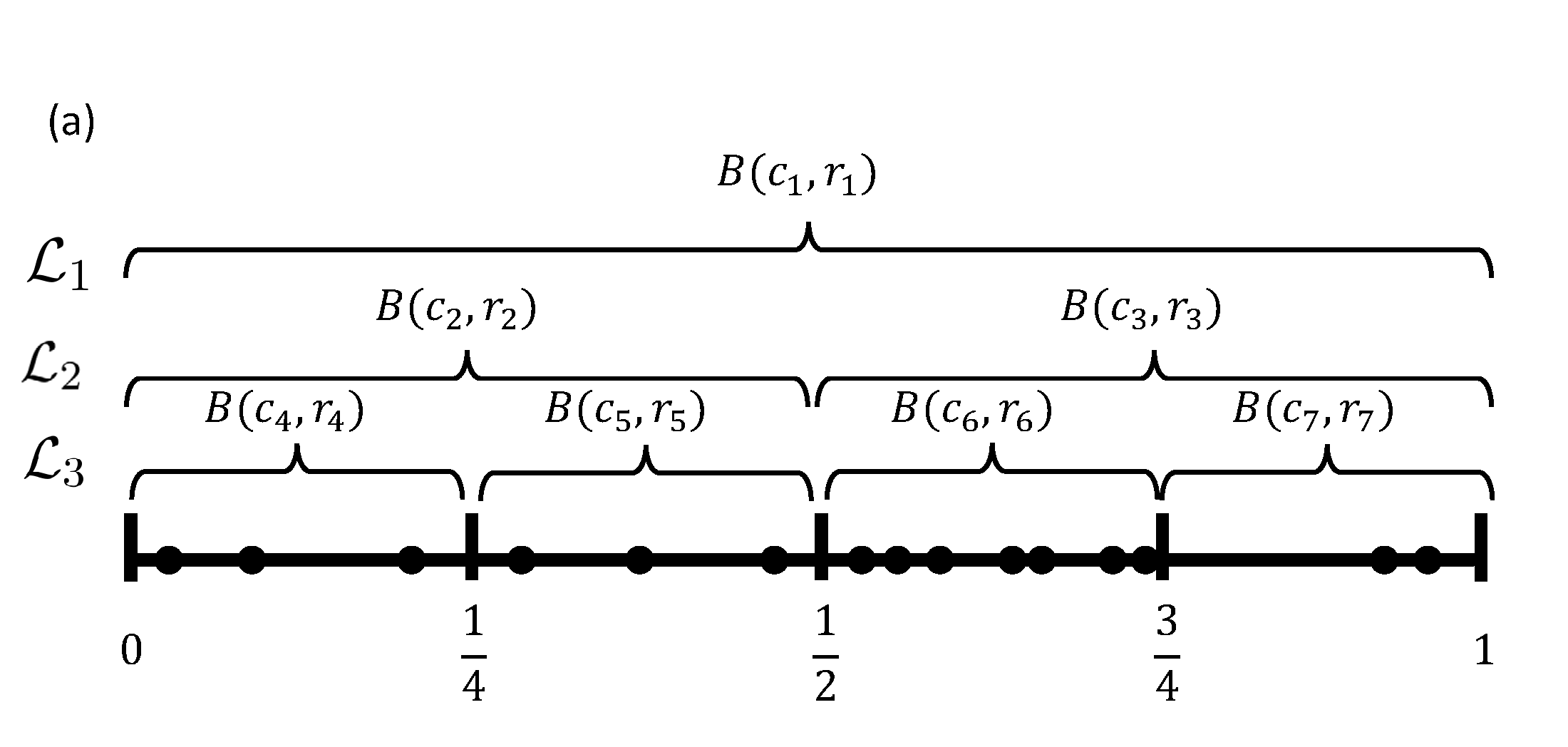
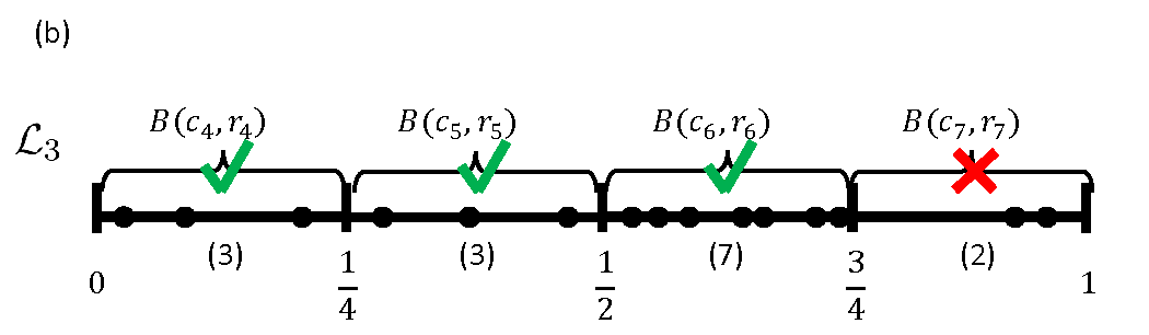
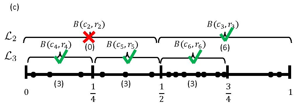
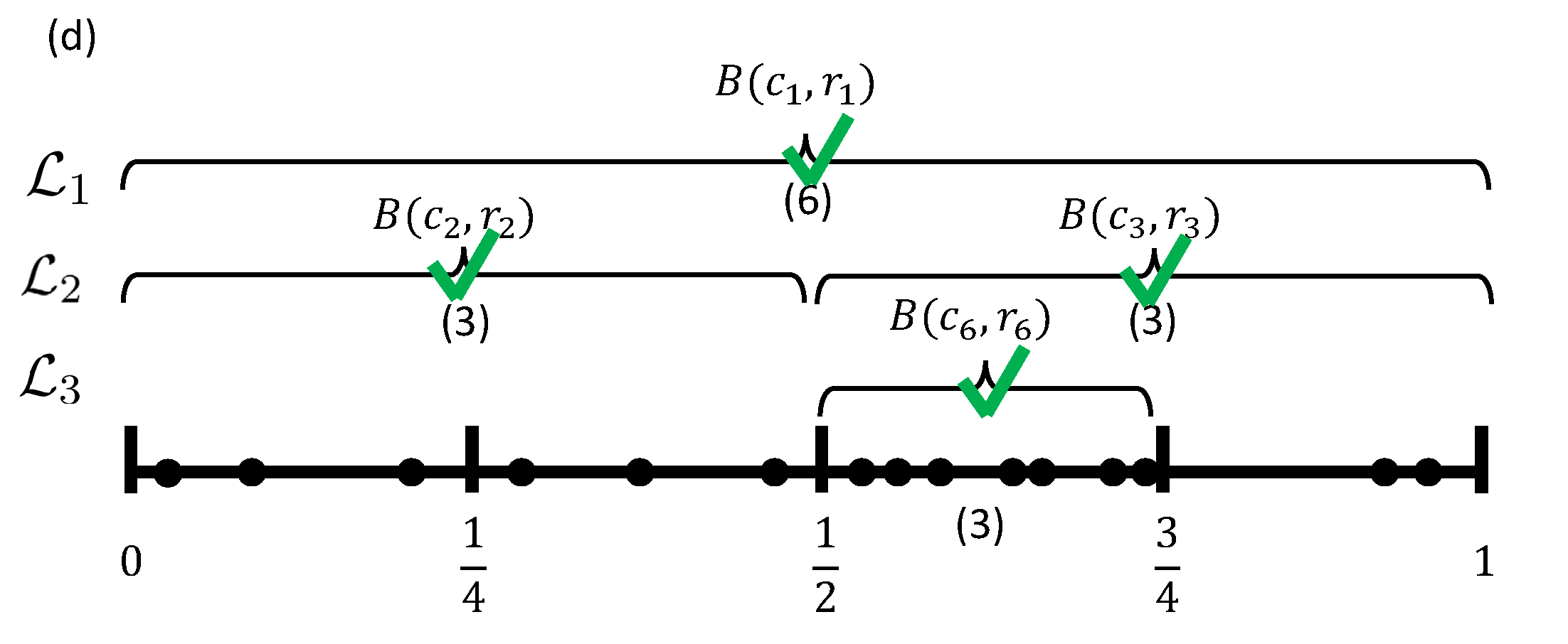
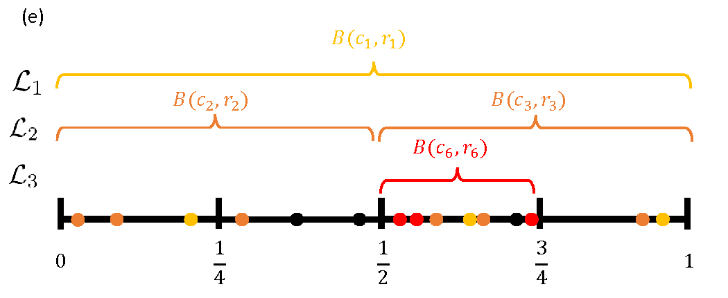
• The initial complete RP scheme as a binary tree with 3-layers on $[0,1]$.

• Starting from layer 3, we prune $B(\boldsymbol{c}_{7},\boldsymbol{w}_{7})$ since there are only $2<3$ observations available. We keep $B(\boldsymbol{c}_{6},\boldsymbol{w}_{6}),B(\boldsymbol{c}_{5},\boldsymbol{w}_{5}),B(\boldsymbol{c}_{4},\boldsymbol{w}_{4})$ as they all contain at least $m=3$ observations.

• Moving to layer 2, $B(\boldsymbol{c}_{3},\boldsymbol{w}_{3})$ has the 6 observations required by itself and its child $B(\boldsymbol{c}_{6},\boldsymbol{w}_{6})$. Checking $B(\boldsymbol{c}_{2},\boldsymbol{w}_{2}),$ it contains only 6 observations so we prune its children $B(\boldsymbol{c}_{4},\boldsymbol{w}_{4}),B(\boldsymbol{c}_{5},\boldsymbol{w}_{5}).$

• Moving to layer 1, $B(\boldsymbol{c}_{1},\boldsymbol{w}_{1})$ contains $15$ observations, therefore there are sufficient observations for $B(\boldsymbol{c}_{1},\boldsymbol{w}_{1})$ and its children $B(\boldsymbol{c}_{2},\boldsymbol{w}_{2})$ , $B(\boldsymbol{c}_{3},\boldsymbol{w}_{3})$ and $B(\boldsymbol{c}_{6},\boldsymbol{w}_{6})$. We keep $B(\boldsymbol{c}_{1},\boldsymbol{w}_{1})$ and its children, completing the partitioning.

• Given the final RP scheme $B(\boldsymbol{c}_{1},\boldsymbol{w}_{1})$, $B(\boldsymbol{c}_{2},\boldsymbol{w}_{2})$, $B(\boldsymbol{c}_{3},\boldsymbol{w}_{3})$ and $B(\boldsymbol{c}_{6},\boldsymbol{w}_{6}),$ one possible random selection of the pseudo-inputs $\bar{\mathcal{X}_{j}}$ for the $j=1,\ldots,N$ different additive components (here $N=4$) conditional on the RP scheme is shown as colored dots. Points with the same color belong to blocks on the same layer.

Figure 1: RP scheme on the domain $\mathsf{X}=[0,1]$ as a $2^{1}$-ary tree with 3 layers and $m=3$ pseudo-inputs per block. The $n=15$ data points $\mathcal{X}$ are represented as dots. The right pane describes the application of the RP pruning Algorithm 1 (a)-(d), and the selection of pseudo-inputs given the RP scheme in (e). The left pane provides the analogous graphical construction of the RP scheme.

To facilitate manipulating and storing the RP scheme on computer, we encode each block by its centroid $\boldsymbol{c}_{j}=(c_{j}^{1},\cdots,c_{j}^{d})$ and half-width $\boldsymbol{w}_{j}=(w_{j}^{1},\ldots,w_{j}^{d})$ where for simplicity we take the half-widths to be the same in each dimension given a layer $l$, $w_{j}^{k}=R_{l},k=1,\ldots,d.$ The $j$-th block is then defined as

$$B_{j}\coloneqq B(\boldsymbol{c}_{j},\boldsymbol{w}_{j})=\left\{\left.\boldsymbol{x}=(x^{1},\ldots,x^{d})\in\mathbb{R}^{d}\right||x^{k}-c_{j}^{k}|\leq w_{j}^{k},k=1,\ldots,d\right\}.$$

We require each block to have a minimum of $m_{j}$ observations, allowing us to later define an SGP with $m_{j}$ pseudo-inputs in each $B_{j}$. For simplicity of exposition, we will assume $m_{j}=m$ for all $j=1,\ldots,N.$ We also require pseudo-inputs $\bar{\mathcal{X}}^{(j)}$ to be mutually disjoint, so that each input setting in $\mathsf{X}$ is chosen as a pseudo-input at most once.

An example RP scheme construction with $L=3$ layers and $m=3$ pseudo-inputs is shown in Figure 1. The construction starts with a complete $2^{d}$-ary tree consisting of layers $\mathcal{L}_{1}=\{B_{1}\},\mathcal{L}_{2}=\{B_{2},B_{3}\}$ and $\mathcal{L}_{3}=\{B_{4},B_{5},B_{6},B_{7}\},$ and a dataset of $n=15$ observations, shown as black dots. Then, the complete tree is pruned according to Algorithm 1, which ensures that each block $B_{j}$ will have at least $m$ pseudo-inputs available while also satisfying therequired properties P1 and P2. Finally, given an RP scheme, one possible random selection of pseudo-inputs is shown.

Algorithm 1 is able to perform the required pruning in general. Essentially, the algorithm works by requiring that the total number of observations in block $B_{j}$ and all of $B_{j}$’s children satisfies the total required number of pseudo-inputs for these components. Starting from the bottom layer, Algorithm 1 recursively works up the tree, pruning sub-trees that do not satisfy this constraint on total number of observations. Once the pruning is complete, the random selection of pseudo-inputs to blocks can be drawn by starting with blocks in layer $L$ and working back to $B_{1},$ thereby guaranteeing that all blocks meet the minimum of $m$ pseudo-inputs per block.

Algorithm 1 Pruning algorithm for RP scheme.

Input :

RP partition scheme $\mathcal{A}$ consisting of $N$ components,   Observed dataset $\{\mathcal{X},\boldsymbol{y}\}$.

Output :

RP partition scheme $\mathcal{A}^{{}^{\prime}}$ consisting of $N^{{}^{\prime}}\leq N$ components,

for $l$ in $L:1$ do

2       for each component $j$ in the $l$-th layer $\mathcal{L}_{l}$ do

3             for $s$ in $L:l$ do

4                   $m_{req}$ $\leftarrow$ Sum of the numbers of pesudo-inputs required for all components contained in $B(\boldsymbol{c}_{j},\boldsymbol{w}_{j})$ in $\mathcal{A}^{{}^{\prime}}$.  if  $\mid\mathcal{X}\cap B(\boldsymbol{c}_{j},\boldsymbol{w}_{j})\mid\geq m_{req}$  then

5                         break 

6                   else

7                         Remove all the children components of component $j$ from the model in $s$-th layer. 

8                   end if

9                  

10             end for

11            

12       end for

13      

14 end for

3.2 SAGP Model

Given a (pruned) RP scheme $\mathcal{B}_{N}$, we propose the additive model (4) for the response $\boldsymbol{y}$, where each component $f_{j}=\left(f_{j}(\boldsymbol{x}_{1}),\ldots,f_{j}(\boldsymbol{x}_{n})\right)^{T}$ is described by an SGP model on the domain $B_{j}$ and $\boldsymbol{\epsilon}\sim N_{n}(\boldsymbol{0}_{n},\sigma_{\epsilon}^{2}\boldsymbol{I}_{n}).$ For block $B(\boldsymbol{c}_{j},\boldsymbol{w}_{j})$, we use $\bar{\mathcal{X}}^{(j)}$ to denote the pseudo-inputs for that block,

$$\bar{\mathcal{X}}^{(j)} =\{\bar{\boldsymbol{x}}_{1}^{(j)},\ldots,\bar{\boldsymbol{x}}_{m_{j}}^{(j)}\}\subset B(\boldsymbol{c}_{j},\boldsymbol{w}_{j})\text{ s.t. }\bar{\boldsymbol{x}}_{k}^{(j)}\in\mathsf{X}\,\forall k.$$

Then, the SGP associated with $\boldsymbol{f}_{j}$ and pseudo-inputs $\bar{\mathcal{X}}^{(j)}$ has corresponding pseudo-targets,

$$\bar{\boldsymbol{f}}_{j} =\left(f_{j}(\bar{\boldsymbol{x}}_{1}^{(j)}),f_{j}(\bar{\boldsymbol{x}}_{2}^{(j)}),\ldots,f_{j}(\bar{\boldsymbol{x}}_{m_{j}}^{(j)})\right)^{T}\in\mathbb{R}^{m_{j}},j=1,\ldots,N.$$ (5)

Then, conditional on the RP scheme and pseudo-inputs, the joint posterior of pseudo-targets and other parameters in (4) can be written as:

$$P(\bar{\boldsymbol{f}}_{1},\ldots,\bar{\boldsymbol{f}}_{N},\boldsymbol{\boldsymbol{\kappa}},\boldsymbol{\sigma}_{\epsilon}^{2}\mid\mathcal{B}_{N},\boldsymbol{y},\mathcal{X},\bar{\mathcal{X}}^{(1)},\ldots,\bar{\mathcal{X}}^{(N)})\propto$$

$$\underbrace{P(\boldsymbol{y}\mid\bar{\boldsymbol{f}}_{1},\ldots,\bar{\boldsymbol{f}}_{N},\boldsymbol{\kappa},\boldsymbol{\sigma}_{\epsilon}^{2},\mathcal{B}_{N},\bar{\mathcal{X}}^{(1)},\ldots,\bar{\mathcal{X}}^{(N)},\mathcal{X})}_{\text{Likelihood Function}}\underbrace{P(\bar{\boldsymbol{f}}_{1},\ldots,\bar{\boldsymbol{f}}_{N}\mid\mathcal{B}_{N},\bar{\mathcal{X}}^{(1)},\ldots,\bar{\mathcal{X}}^{(N)},\mathcal{X},\boldsymbol{\boldsymbol{\kappa}})}_{\text{Pseudo-target Prior}}\times$$

$$\underbrace{P(\boldsymbol{\boldsymbol{\kappa}}\mid\mathcal{B}_{N})}_{\text{Kernel Prior}}\underbrace{P(\boldsymbol{\sigma}_{\epsilon}^{2})}_{\text{Error Prior}}.$$ (6)

In effect, we view the choice of pseudo-inputs $\bar{\mathcal{X}}^{(1)},\ldots,\bar{\mathcal{X}}^{(N)}$ as nuisance parameters, and ultimately will integrate them out with respect to the prior $P(\bar{\mathcal{X}}^{(1)},\ldots,\bar{\mathcal{X}}^{(N)}\mid\mathcal{B}_{N})$, which gives the marginal posterior of interest,

$$P(\bar{\boldsymbol{f}}_{1},\ldots,\bar{\boldsymbol{f}}_{N},\boldsymbol{\boldsymbol{\kappa}},\boldsymbol{\sigma}_{\epsilon}^{2}\mid\mathcal{B}_{N},\boldsymbol{y},\mathcal{X}) =$$

$$\int P(\bar{\boldsymbol{f}}_{1},\ldots,\bar{\boldsymbol{f}}_{N},\boldsymbol{\boldsymbol{\kappa}},\boldsymbol{\sigma}_{\epsilon}^{2}\mid\mathcal{B}_{N},\boldsymbol{y},\mathcal{X},\bar{\mathcal{X}}^{(1)},\ldots,\bar{\mathcal{X}}^{(N)}) \underbrace{P(\bar{\mathcal{X}}^{(1)},\ldots,\bar{\mathcal{X}}^{(N)}\mid\mathcal{B}_{N})}_{\text{Pseudo-input Prior}}d\bar{\boldsymbol{x}}^{m_{1}}\ldots d\bar{\boldsymbol{x}}^{m_{N}},$$

where $d\bar{\boldsymbol{x}}^{m_{j}}=d\bar{\boldsymbol{x}}_{1}^{(j)}\times\ldots\times d\bar{\boldsymbol{x}}_{m_{j}}^{(j)}.$

In subsection 3.2.7 we will show a Gibbs sampler algorithm for SAGP fitting and for calculating predictions, but first we describe in greater detail the likelihood function and various prior distributions involved in the SAGP model.

3.2.1 Likelihood Function, $P({\boldmath y}\mid\bar{\boldmath{f}}_{1},\ldots,\bar{\boldmath{f}}_{N},\boldsymbol{\kappa},\sigma_{\epsilon}^{2},\mathcal{B}_{N},\bar{\mathcal{X}}^{(1)},\ldots,\bar{\mathcal{X}}^{(N)},\mathcal{X})$

Let us denote the covariance kernel for the SGP in the $j$-th block by $K^{(j)},j=1,\ldots,N$ . We use the Gaussian covariance kernel supported inside $B_{j}$ with parameters $\boldsymbol{\kappa}^{(j)}=(\rho^{(j)},\eta^{(j)})$. We have

$$K^{(j)}(\boldsymbol{x},\boldsymbol{x}^{\prime}) \coloneqq\frac{1}{\eta^{(j)}}\cdot\left(\rho^{(j)}\right)^{\left[(\boldsymbol{x}-\boldsymbol{x}^{\prime})^{T}(\boldsymbol{x}-\boldsymbol{x}^{\prime})\right]},\forall\boldsymbol{x},\boldsymbol{x}^{\prime}\in B_{j}.$$ (7)

Using (7), we can write down the (cross-)covariance matrices among and between inputs in $\mathcal{X}$ and $\bar{\mathcal{X}}^{(j)}$ as:

$$\boldsymbol{K}_{n}^{(j)} \coloneqq\left[K^{(j)}(\boldsymbol{x}_{k},\boldsymbol{x}_{l})\right]_{k,l=1}^{n},$$

$$\boldsymbol{K}_{m_{j}}^{(j)} \coloneqq\left[K^{(j)}(\bar{\boldsymbol{x}}_{k}^{(j)},\bar{\boldsymbol{x}}_{l}^{(j)})\right]_{k,l=1}^{m_{j}},$$

$$\boldsymbol{K}_{nm_{j}}^{(j)} \coloneqq\left[K^{(j)}(\boldsymbol{x}_{k},\bar{\boldsymbol{x}}_{l}^{(j)})\right]_{k,l=1}^{n,m_{j}}=\left(\boldsymbol{K}_{m_{j}n}^{(j)}\right)^{T}.$$

For a general $\boldsymbol{x}\in\mathbb{R}^{d},$ we also have

$$\boldsymbol{k}_{\boldsymbol{x}}^{(j)} \coloneqq\left(\begin{array}[]{ccc}K^{(j)}(\bar{\boldsymbol{x}}_{1}^{(j)},\boldsymbol{x}),&\ldots&,K^{(j)}(\bar{\boldsymbol{x}}_{m_{j}}^{(j)},\boldsymbol{x})\end{array}\right)^{T}.$$ (9)

Assuming the additive components are conditionally independent, the likelihood is (see Lemma 1 in Appendix D)

$$P(\boldsymbol{y}\mid\boldsymbol{\bar{f}}_{1},\ldots,\bar{\boldsymbol{f}}_{N},\boldsymbol{\boldsymbol{\kappa}},\boldsymbol{\sigma}_{\epsilon}^{2},\mathcal{B}_{N},\bar{\mathcal{X}}^{(1)},\ldots,\bar{\mathcal{X}}^{(N)}) =N_{n}\left(\boldsymbol{y}\left|\sum_{j=1}^{N}\boldsymbol{K}_{nm_{j}}^{(j)}\left(\boldsymbol{K}_{m_{j}}^{(j)}\right)^{-1}\bar{\boldsymbol{f}}_{j},\sigma_{\epsilon}^{2}\boldsymbol{I}_{n}+\sum_{j=1}^{N}\boldsymbol{\Lambda}_{n}^{(j)}\right.\right)$$ (10)

where the matrix $\boldsymbol{\Lambda}_{n}^{(j)}\coloneqq\text{diag}\left(K_{ii}^{(j)}-\boldsymbol{k}_{i}^{(j)T}\left(\boldsymbol{K}_{m_{j}}^{(j)}\right)^{-1}\boldsymbol{k}_{i}^{(j)}\right)_{n\times n}$ takes the diagonal form, with $\boldsymbol{k}_{i}^{(j)}$ as defined in (9) (with subscript $i$ being shorthand for $\boldsymbol{x}_{i}$).

3.2.2 Pseudo-target Prior, $P(\bar{\boldmath{f}}_{1},\ldots,\bar{\boldmath{f}}_{N}\mid\mathcal{B}_{N},\bar{\mathcal{X}}^{(1)},\ldots,\bar{\mathcal{X}}^{(N)},\mathcal{X},\boldmath{\kappa})$

The prior distribution of pseudo-targets given pseudo-inputs and covariance function parameters is straight-forward. Following Snelson and Ghahramani (2006), the pseudo-targets are assumed to be a priori conditionally independent, and sohave Gaussian distributions with prescribed kernels:

$$P(\bar{\boldsymbol{f}}_{1},\ldots,\bar{\boldsymbol{f}}_{N}\mid\mathcal{B}_{N},\bar{\mathcal{X}}^{(1)},\ldots,\bar{\mathcal{X}}^{(N)},\mathcal{X},\boldsymbol{\boldsymbol{\kappa}}) =\prod_{j=1}^{N}P(\bar{\boldsymbol{f}}_{j}\mid\mathcal{B}_{N},\bar{\mathcal{X}}^{(j)},\mathcal{X},\boldsymbol{\boldsymbol{\kappa}}^{(j)})$$

$$=\prod_{j=1}^{N}N_{m_{j}}\left(\bar{\boldsymbol{f}}_{j}\left|\boldsymbol{0}_{m_{j}},\boldsymbol{K}_{m_{j}}^{(j)}\right.\right).$$ (11)

3.2.3 Pseudo-input Prior, $P(\bar{\mathcal{X}}^{(1)},\ldots,\bar{\mathcal{X}}^{(N)}\mid\mathcal{B}_{N},\mathcal{X})$

The idea of the proposed pseudo-input prior is to sample pseudo-inputs uniformly within each block $B_{j}$ while satisfying properties P1–P3 required for the RP scheme, $\mathcal{B}_{N}.$ Algorithm 2 implements such a sampling scheme, which we now motivate. Let the index set $\mathcal{I}_{j}$ representing the indices of children blocks of block $B_{j}$, which is defined as

$$\mathcal{I}_{j} \coloneqq\{k\neq j\text{ such that }B_{k}\subset B_{j}\},$$

and also define the collection of already selected pseudo-inputs of these child blocks as $\mathcal{C}(B_{j})\coloneqq\cup_{k\in\mathcal{I}_{j}}\bar{\mathcal{X}}^{(k)}.$ Then,

$$P(\bar{\mathcal{X}}^{(1)},\ldots,\bar{\mathcal{X}}^{(N)}\mid\mathcal{B}_{N}) =\prod_{\ell=L}^{1}\prod_{j:B_{j}\in\mathcal{L}_{\ell}}P(\bar{\mathcal{X}}^{(j)}\mid\mathcal{C}(B_{j}))$$

where

$$P(\bar{\mathcal{X}}^{(j)}\mid\mathcal{C}(B_{j})) =\prod_{i=1}^{m_{j}}P(\bar{\boldsymbol{x}}_{i}^{(j)}\mid\mathcal{C}(B_{j}))$$

and

$$P(\bar{\boldsymbol{x}}_{i}^{(j)}\mid\mathcal{C}(B_{j})) =\text{Discrete Uniform}\left(\left\{\boldsymbol{x}\in\mathcal{X}\subset B_{j}\backslash\mathcal{C}(B_{j})\right\}\right).$$

In the expression above, we essentially draw a random sample from all those observed locations that have not been selected as pseudo-inputs of any children components in the lower layers of the RP scheme.

Unlike the standard SGP approach, this allows us to capture the uncertainty of pseudo-input selection by sampling the pseudo-inputs using Algorithm 2 and propagating this uncertainty to the posterior. Alternatives such as a continuous uniform prior over each component domain $B_{j}$, or sampling accordingly to design-theoretic considerations (Pratola et al., 2019), are possible.

Algorithm 2 Sampling pseudo-inputs given RP scheme $\mathcal{B}_{N}$.

Input :

RP scheme $\mathcal{B}_{N}$ consisting of $N$ blocks,   Observed inputs $\mathcal{X}$.

Output :

Sample of $\bar{\mathcal{X}}^{(j)},j=1,\ldots,N$ conditional on RP scheme $\mathcal{B}_{N}$.

Initialize $\mathcal{X}_{A}=\mathcal{X}$ as available inputs.

for $j$ in $N:1$ do

2       Sample a random sample $\bar{\mathcal{X}}^{(j)}\subset\mathcal{X}\subset\mathbb{R}^{d}$ of size $m_{j}$ from $\mathcal{X}\cap B_{j}\cap\mathcal{X}_{A}$.  $\mathcal{X}_{A}\leftarrow\mathcal{X}_{A}\setminus\bar{\mathcal{X}}^{(j)}$ // Remove $\bar{\mathcal{X}}^{(j)}$ sampled in the previous step from $\mathcal{X}_{A}$. 

3 end for

3.2.4 Additional Prior Distributions, $P(\boldsymbol{\kappa}\mid\mathcal{B}_{N})$ and $P(\sigma_{\epsilon}^{2})$

We place a conjugate inverse gamma prior on the noise variance, $\sigma_{\epsilon}^{2}$,

$$\sigma_{\epsilon}^{2} \sim\text{InverseGamma}(\alpha_{\epsilon},\beta_{\epsilon}).$$

The hyper-parameters $\alpha_{\epsilon}$ and $\beta_{\epsilon}$ may be chosen as the hyper-parameters of the noise variance in traditional Bayesian GP regression.

We assume independent priors on the scale and correlation parameters of the kernel, $\eta^{(j)}$ and $\rho^{(j)}$,

$$P(\boldsymbol{\boldsymbol{\kappa}}) =P(\boldsymbol{\boldsymbol{\kappa}}^{(1)},\ldots,\boldsymbol{\boldsymbol{\kappa}}^{(j)})=\prod_{\ell=1}^{L}\prod_{B_{j}\in\mathcal{L}_{\ell}}P(\eta^{(j)}\mid\alpha_{\eta}^{l},\beta_{\eta}^{l})P(\rho^{(j)}).$$

The precision parameters $\eta^{(j)}$ are assumed to have gamma priors,

$$\eta^{(j)} \sim\text{Gamma}(\alpha_{\eta}^{l},\beta_{\eta}^{l}),$$

with $\alpha_{\eta}^{l},\beta_{\eta}^{l}>0,l=1,\ldots,L$. The hyper-parameters $\alpha_{\eta}^{l},\beta_{\eta}^{l}$ are the same for components within the same layer. We set up these hyper-parameters so that the variance of the response explained by the SAGP model is unequally partitioned across the $L$ layers, with components in higher layers of the partitioning scheme explaining larger portions of the variance. To facilitate the set-up of the hyper-parameters, we first normalize the observed responses $y_{1},\ldots,y_{n}$, re-centering and re-scaling so that they have mean 0 and variance 1. For all the components in layer $l$, we set

$$\alpha_{\eta}^{l}= \mathsf{c}_{1\eta}+1,$$

$$\beta_{\eta}^{l}= \mathsf{c}_{1\eta}(1-\mathsf{c}_{2\eta})\mathsf{c}_{2\eta}^{l-1},$$

with $\mathsf{c}_{1\eta}>0$ and $0<\mathsf{c}_{2\eta}<1$. For each component $j$ in layer $l$, this choice implies that $1/\eta^{(j)}$, the marginal variance of the component, has prior mean

$$E[1/\eta^{(j)}]= \frac{\beta_{\eta}^{l}}{\alpha_{\eta}^{l}-1}=(1-\mathsf{c}_{2\eta})\mathsf{c}_{2\eta}^{l-1}.$$

For example, if $\mathsf{c}_{2\eta}=.1$, components on layer $l=1$ are expected to have variance $1-\mathsf{c}_{2\eta}=.9$, which is 90$\%$ of the variance of the response because of the normalization. Components on layer $l=2$ are expected to have $(1-\mathsf{c}_{2\eta})\mathsf{c}_{2\eta}=0.09$, 9$\%$ of the variance of the response. Similarly, as $l$ increases, components are expected to explain smaller portions of the variance of the response. In particular, the geometric decay of the prior mean of $1/\eta^{(j)}$ is chosen so that the expected layer-specific variances add up to approximately the total response variance, which is guaranteed because, if $L$ is sufficiently big, $\sum_{l=1}^{L}(1-\mathsf{c}_{2\eta})\mathsf{c}_{2\eta}^{l-1}\approx 1$. The other hyper-parameter $\mathsf{c}_{1\eta}$ controls the spread of the prior distributions of $1/\eta^{(j)}$, with larger values of $\mathsf{c}_{1\eta}$ imposing a tighter constraint to the prior mean. In our experience, values of $\mathsf{c}_{2\eta}=.1$ and $\mathsf{c}_{1\eta}$ between 10 and 50 appear to provide the best results in our applications.

We set the prior distributions on the parameters $\rho^{(j)}$ in the following way. First of all, we assume that the inputs $\boldsymbol{x}_{i}$’s have been appropriately scaled, so that the domain $\mathsf{X}$ is mapped into the unit cube $[0,1]^{d}$. This facilitates the definition of priors for $\rho^{(j)}$. Second, as for the $\eta^{(j)}$, we assume the same prior distribution for parameters corresponding to components in the same layer $l$. Third, we adopt a structure of priors imposing smoother behavior for components in the top layers of the partitioning scheme. In other words, we impose a structure of priors where $\rho^{(j)}$ is expected to be greater than $\rho^{(j^{\prime})}$ if component $j$ belongs to a layer on a higher level than the layer of component $j^{\prime}$. Despite a family of beta priors on the $\rho^{(j)}$ may be tuned to satisfy these properties, we empirically observed that setting the values of these parameters to fixed layer-specific constants $\rho_{l}$ (i.e., $P(\rho^{(j)})=\delta_{\rho_{l}}$, the Dirac delta function on $\rho_{l}$) worked as well but was computationally less expensive. To get the sense on how the values of $\rho_{l}$ affect the layer-specific correlations, one may plot the correlation for two responses as a function of the distance of their inputs, as specified by Equation (7). We provide this plot in Appendix A, in the case $L=5$ and using the values $\rho_{1}=10^{-1}$, $\rho_{L}=10^{-50}$ and the intermediate values $\rho_{l},l=2,\ldots,L-1$ to be equally spaced between $\rho_{1}$ and $\rho_{L}$ on the logarithm (base 10) scale. Even though these values of $\rho_{l}$ may appear to quickly become excessively small, the sizes of the subdomains where the components are defined (i.e., the blocks $B_{j}$) shrink as $l$ increases. In our numerical example, if we consider a one-dimensional case with two inputs $\boldsymbol{x}$ and $\boldsymbol{x}^{\prime}$ at distance 0.0625 (i.e., the largest distance between two points in one block on the fifth layer), the assumed correlations on components on layer $l=1$ to 5 are 0.99, 0.89, 0.80, 0.71 and 0.64, respectively. Notably, the decay of such values depends on the number of layers $L$, which can be tuned using prior beliefs and the information in the data. In our applications, trading the conventional estimation of the parameters $\rho^{(j)}$ with a set of fixed $\rho_{l}$ and a data-driven selection of $L$ via cross-validation (see Section 3.2.8) resulted in sufficiently flexible models.

3.2.5 Full Conditional Distribution of Pseudo-targets

In order to implement an MCMC algorithm for SAGP, we apply Bayes theorem on the pseudo-inputs $\bar{\boldsymbol{f}}_{j}$ in order to yield its full conditional distribution from (10) and (11) and the conditional independence assumption,

$$P(\bar{\boldsymbol{f}}_{j}\mid\boldsymbol{y},\mathcal{X},\bar{\boldsymbol{f}}_{1},\ldots,\bar{\boldsymbol{f}}_{j-1},\bar{\boldsymbol{f}}_{j+1},\ldots\bar{\boldsymbol{f}}_{N},\mathcal{B}_{N},\bar{\mathcal{X}}^{(1)},\ldots,\bar{\mathcal{X}}^{(N)},\boldsymbol{\boldsymbol{\kappa}},\boldsymbol{\sigma}_{\epsilon}^{2})$$

$$\propto P(\boldsymbol{y}\mid\bar{\boldsymbol{f}}_{1},\ldots\bar{\boldsymbol{f}}_{N},\mathcal{B}_{N},\bar{\mathcal{X}}^{(1)},\ldots,\bar{\mathcal{X}}^{(N)},\boldsymbol{\boldsymbol{\kappa}},\boldsymbol{\sigma}_{\epsilon}^{2})\times$$

$$P(\bar{\boldsymbol{f}}_{j}\mid\mathcal{X},\mathcal{B}_{N},\bar{\mathcal{X}}^{(j)},\boldsymbol{\boldsymbol{\kappa}},\boldsymbol{\sigma}_{\epsilon}^{2})$$

$$=N_{n}\left(\left.\boldsymbol{r}_{j}\right|\boldsymbol{K}_{nm_{j}}^{(j)}\left(\boldsymbol{K}_{m_{j}}^{(j)}\right)^{-1}\bar{\boldsymbol{f}}_{j},\boldsymbol{\Lambda}_{n}^{(j)}+\sigma_{\epsilon}^{2}\boldsymbol{I}_{n}\right)\times N_{m_{j}}\left(\left.\bar{\boldsymbol{f}}_{j}\right|\boldsymbol{0}_{m_{j}},\boldsymbol{K}_{m_{j}}^{(j)}\right),$$ (12)

where $\boldsymbol{r}_{j}=\boldsymbol{y}-\sum_{l\neq j}\boldsymbol{K}_{nm_{l}}^{(l)}\left(\boldsymbol{K}_{m_{l}}^{(l)}\right)^{-1}\bar{\boldsymbol{f}}_{l}.$ Using normal-normal conjugacy, we can identify the mean and variance of this normal distribution, $\bar{\boldsymbol{f}}_{j}\mid\boldsymbol{Mean}_{j},\boldsymbol{Var}_{j}$, where (see Appendix D)

$$\boldsymbol{Mean}_{j} =\boldsymbol{K}_{m_{j}}^{(j)}\boldsymbol{Q}_{m_{j}}^{(j)-1}\boldsymbol{K}_{m_{j}n}^{(j)}\left(\boldsymbol{\Lambda}_{n}^{(j)}+\sigma_{\epsilon}^{2}\boldsymbol{I}_{n}\right)^{-1}\boldsymbol{r}_{j},$$

$$\boldsymbol{Var}_{j} =\boldsymbol{K}_{m_{j}}^{(j)}\boldsymbol{Q}_{m_{j}}^{(j)-1}\boldsymbol{K}_{m_{j}}^{(j)},$$

$$\text{and }\boldsymbol{Q}_{m_{j}}^{(j)}= \boldsymbol{K}_{m_{j}}^{(j)}+\boldsymbol{K}_{m_{j}n}^{(j)}\left(\boldsymbol{\Lambda}_{n}^{(j)}+\sigma_{\epsilon}^{2}\boldsymbol{I}_{n}\right)^{-1}\boldsymbol{K}_{nm_{j}}^{(j)}.$$ (13)

Although we still need to invert an $n\times n$ matrix $\boldsymbol{\Lambda}_{n}^{(j)}+\sigma_{\epsilon}^{2}\boldsymbol{I}_{n}$, it is a diagonal matrix and hence its computational cost will be $\mathcal{O}(n)$.

3.2.6 Full Conditional Distribution of Noise Variance

As we mentioned in the previous section, we want to make use of the Gaussian-inverse gamma conjugacy. For the observation of sample size $n$, by conjugacy, the distribution $\sigma_{\epsilon}^{2}$ is again inverse gamma,

$$P(\sigma_{\epsilon}^{2}\mid\boldsymbol{y},\mathcal{X},\bar{\boldsymbol{f}}_{1},\ldots\bar{\boldsymbol{f}}_{N},\mathcal{B}_{N},\bar{\mathcal{X}}^{(1)},\ldots,\bar{\mathcal{X}}^{(N)},\boldsymbol{\boldsymbol{\kappa}})=$$

$$\text{InverseGamma}\left(\alpha_{\epsilon}+\frac{n}{2},\beta_{\epsilon}+\frac{1}{2}(\boldsymbol{y}-\hat{\boldsymbol{y}})^{T}(\boldsymbol{y}-\hat{\boldsymbol{y}})\right),$$

where $\hat{\boldsymbol{y}}\coloneqq\sum_{j=1}^{N}\boldsymbol{K}_{nm_{j}}^{(j)}\left(\boldsymbol{K}_{m_{j}}^{(j)}\right)^{-1}\bar{\boldsymbol{f}}_{j}$ is the “fitted value” from the SAGP model. We can directly sample this parameter using a Gibbs step.

3.2.7 Sampling Algorithm

SAGP is fitted by a Metropolis-Hastings Markov chain Monte Carlo (MCMC) algorithm (Alan E. Gelfand, 1990). For each additive component of the model, we have to use the partial residuals $\boldsymbol{r}_{j}$ defined in (12) as data. This step is from the back-fitting scheme designed for fitting additive Bayesian models (Hastie and Tibshirani, 2000).

From the likelihood derivations presented in section 3.2.5, we know that $\bar{\boldsymbol{f}_{j}}$ can be directly sampled from their conditional distributions for each $j=1,\ldots,N$ components. The difficulty in this step is to compute the $\boldsymbol{Mean}_{j},\boldsymbol{Var}_{j}$ in (13). As mentioned earlier, the main computational cost occurs in the inversion of the covariance matrices in section 3.2.1, which has been reduced compared to a full GP covariance matrix. Numerical instability in inversion of these matrices may cause additional problems, so we adopt the Cholesky decomposition method with diagonal perturbation to solve this instability problem as in Rasmussen and Williams (2006). For each $\eta_{j}$ we do not have normal conjugacy, therefore an adaptive Metropolis-Hasting step is used for sampling $\eta_{j}$ (Banerjee et al., 2012).

The advantage of using such a fully Bayesian model is that the uncertainty quantification comes naturally with the posterior samples from the sampler. Our posterior inference below can be based on all these posterior samples. The algorithm for overall sampling is presented in Algorithm 3 in the Appendix C.

3.2.8 Tuning Parameters and Complexity

The trade-off between number of layers $L$ in the RP scheme and the number of pseudo-inputs $m$ is central to the SAGP model. On one hand, in SGP modeling (Snelson and Ghahramani, 2006, 2007; Lee et al., 2017), we need to increase the number of pseudo-inputs $m$ to get a better fit of the SGP model. On the other hand, for regression tree partitionining models (Chipman et al., 1998, 2016; Pratola et al., 2018), the more additive components a model has, the better fit we can expect. In the SAGP model, increasing both factors (number of pseudo-inputs, $m,$ and number of layers, $L,$) would certainly improve the overall fit, but the interesting observation is that there exists a trade-off between these two tuning parameters. Increasing the number of layers $L$ may counter-act the effect of decreasing the number of pseudo-inputs $m$, and vice versa. Theoretically, we can tune the choice of number of layers using cross-validation (see Figure 4). Practically, we can usually choose reasonable $m$ and $L$ depending on the desired granularity of the RP scheme.

This trade-off between $m$ and $L$ can also be observed by considering the model’s computational complexity. We already mentioned above that for a full GP model based on $\mathcal{X}$ the complexity is of order $\mathcal{O}(n^{3})$; for an SGP model with $m\ll n$ pseudo-inputs selected from $\mathcal{X},$ the complexity is of order $\mathcal{O}(nm^{2})$ (Snelson and Ghahramani, 2006). Since each additive component in our SAGP model is essentially an SGP model, the overall complexity is given by the following proposition.

Proposition 1

For an RP scheme on input-domain $[0,1]^{d}$, with $b_{i}$-ary tree (Storer, 2012) in the $i$-th dimension, the complexity of fitting an $L$-layer SAGP model with $m$ pseudo-inputs for each block and an overall sample of size $n$ is at most $\mathcal{O}\left(\sum_{\ell=1}^{L}\prod_{i=1}^{d}b_{i}^{\ell-1}\cdot n\cdot m^{2}\right)$.

Proof  See Appendix B.  
For $N=1$, where there is only one layer and one component, this complexity reduces to SGP complexity with $m$ pseudo-inputs. We will revisit this component number pseudo-input trade-off in our data analyses.

4 Simulation Study

4.1 Design

To evaluate the performance of our methodology and compare it to competing approaches, we run a family of simulations. We focus on the one-dimensional case ($d=1$) and we simulate from a GP with mean function

$$f(x)=-5-6x^{3}+30(x-.5)^{2}+3\exp(2x-1)+3x^{2}\sin(12\pi x)+\cos(6\pi x),$$ (14)

which is represented in Figure 2 in the interval [0,1]. We generate a sample of $n=200$ locations from a uniform distribution on $[0,1]$ and we define the observed responses as $y_{i}=f(x_{i})+\epsilon_{i}$ for all $x_{i}\in\mathcal{X}$, with $\epsilon_{i}\sim N_{1}(0,0.1)$. The data are split into training and testing sets, with sizes 150 and 50, respectively. We consider two scenarios. In the first scenario, the testing set is selected at random. In the second scenario, the testing set is chosen as the subset with 50 data points with $x_{i}$ closest to a point randomly chosen in $[0.25,0.75]$. Figure 2 shows an example for each of these scenarios.

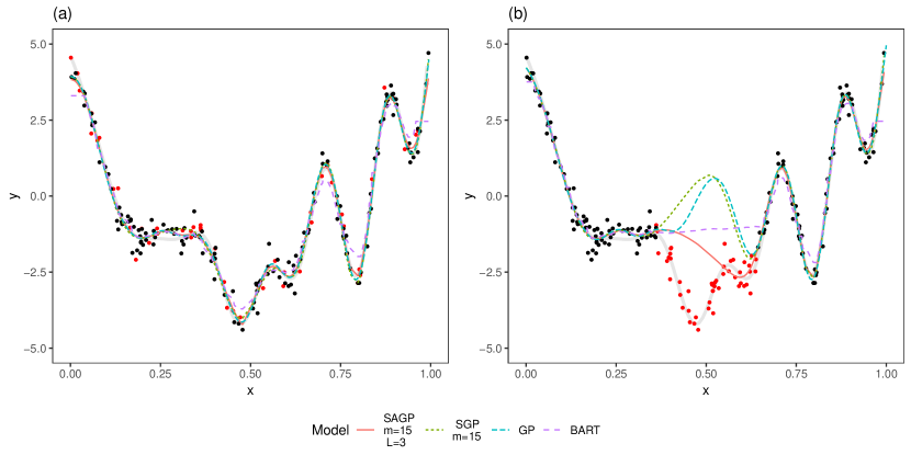
Figure 2: Example of data generated in the simulation study. The gray, bold, curve represents the true mean function $f(x)$. Training and testing sets are represented as black and red points. Panels (a) and (b) show the scenarios where the 50 data points of the testing set are chosen at random or as the input location that is closest to a randomly chosen point (0.5 in the example), respectively. The posterior predictive functions of four models, fit on the training portion of the data, are provided in both panels.

We generate 1000 datasets for each scenario (random and interval testing set). In each dataset, we fit the SAGP model with three configurations of $m,L$: (i) $m=5$, $L=4$; (ii) $m=10$, $L=3$; (iii) $m=15$, $L=3$. We compare the SAGP models to the following methods:

• Full GP regression. We use the implementation of GP regression model in the R package $\mathtt{DiceKriging}$ by Roustant et al. (2012).

• SGP regression. We consider the choices $m=5$, $m=10$ and $m=15$ and use the implementation of SGP in the Matlab package implementation $\mathtt{SPGP}$ at http://www.gaussianprocess.org accompanying the paper by Snelson and Ghahramani (2006).

• Bayesian Additive Regression Trees (BART) Chipman et al. (1998, 2010); Pratola et al. (2018). We used the default number of trees as specified in Chipman et al. (2010) and the implementation at http://bitbucket.org/mpratola/openbt.

For each generated dataset, the models are fit on the training data and used to predict the response on the testing data. For each point in the testing set, we compute the estimated mean function $\hat{y}(x_{i})$ (see Section 3.2.6) and the 95$\%$ prediction interval (PI) for $y_{i}$. The performance of the estimators of the mean function is evaluated in terms of root mean squared error (RMSE). To assess the appropriateness of the uncertainty quantification, we compute the coverage of the PIs and compare it to the nominal prediction level. Finally, we compare the methods in terms of average value of interval score, which is a summary measure to assess the quality of prediction intervals (Gneiting and Raftery, 2007). Given a $(1-\alpha)100\%$ PI for $y_{i}$ with extremes $(l_{i},u_{i})$, the interval score at $y_{i}$ is defined as

$$s_{\alpha}(l_{i},u_{i};y_{i})=(u_{i}-l_{i})+\frac{2}{\alpha}(l_{i}-y_{i})\boldsymbol{1}(y_{i}<l_{i})+\frac{2}{\alpha}(y_{i}-u_{i})\boldsymbol{1}(y_{i}>u_{i}).$$

We choose this metric to jointly evaluate a family of intervals in terms of precision (i.e. the width of the intervals) and accuracy (i.e., the coverage of the true value). Notably, low values of the score indicate good performance.

4.2 Results

Figure 3 summarizes the resulting RMSEs, PI coverages and averages of the interval scores across the 1000 generated datasets for the two scenarios.

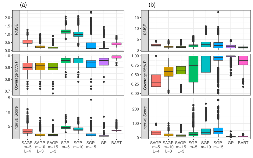
Figure 3: RMSE (top panels), coverage (central panels) and interval score (bottom panels) over the 1000 simulated datasets. Panel (a) shows the results in the case where the testing set is chosen at random over $[0,1]$. Panel (b) shows the results in the case where the testing set is chosen in a random interval with center uniformly selected from $[0.25,0.75]$.

Panel (a) provides the results in the scenario where the testing set is selected at random. In terms of RMSE, both the SAGP and SGP models perform better with larger values of $m$. As expected, the full GP model attains the smallest RMSEs. The SAGP models with $m=5$ and 10 perform better than the SGP models with the same number of pseudo-inputs. For $m=15$, the median RMSEs in the SAGP and SGP models are similar, but the performance of the SAGP model is more consistent across simulations (the upper quartile of SAGP with $m=15$ is considerably smaller than the one of SGP with $m=15$). With the considered configuration of the parameters, the BART model performs slightly better than the SAGP model with $m=5$, but worse than the SAGP model with $m=10$ and $m=15$. The coverage of the 95$\%$ PIs is close to the nominal level for all the methods except for BART. The PIs of the SAGP model appear to be slightly too narrow, as most of the coverages are a little lower than .95. SGP and GP models show coverages perfectly matching the nominal value. However, the BART model produces overly wide PIs, as the median coverage is 100$\%$. The ranking of the methods in terms of interval score is similar to the one based on the RMSE. Again, better performances are attained by SAGP and SGP models with larger values of $m$. The SAGP models with $m=10$ and $m=15$ perform better than all the other methods, except for the full GP model.

Panel (b) provides the results of the simulations in the scenario where the testing set is an interval with random mid-point. Notably, this prediction problem is much harder than the one evaluated by the previous scenario, as the models are forced to a certain degree of extrapolation due to the lack of data. BART, GP and SAGP with $m=15$ attain the best performance in terms of RMSE. Overall, the SAGP model seem to perform better than SGP. The coverage is suboptimal for all the methods, being much lower (undercoverage) than expected for SAGP and SGP with $m=5$ and higher (overcoverage) for GP. A wide range of coverages is observed for all the other methods. With respect to the interval score, GP and BART are the methods that appear to perform best. Among the SAGP and SGP models, SAGP with $m=15$ is the best performing and competitive with GP and BART.

4.3 Computational Details

As for any Bayesian model that is fit using MCMC algorithms, the convergence to the stationary distribution must be investigated also for the SAGP model. In our specific implementation, we discard the first 10,000 samples as burn-in and keep the following 1,000 samples to compute posterior estimates. We monitor the convergence of $\sigma^{2}_{\epsilon}$, sampled with Gibbs steps, and of the parameters $\eta^{(j)}$, which are sampled with Metropolis-Hastings steps with an adaptive choice of the bandwidth of the proposal distribution to control the acceptance rate. The considered SAGP models turned out to mix well and reasonably fast on the basis of trace-plots of the parameters (not shown) and the diagnostics suggested by Gelman et al. (2013), which are provided in Appendix E. Notably, in our experience, similar satisfying mixing diagnostic for the SAGP model may be achieved with much fewer steps than 10,000.

Table 1: Computation time needed to fit the SAGP model on 1,000 simulated datasets on a 40-core cluster.

$m$	$L$	Testing set	CPU time (hh:mm:ss)
10	3	Random	106:53:21
10	3	Interval	107:56:21
5	4	Random	241:17:31
5	4	Interval	175:45:35
15	3	Random	477:22:52
15	3	Interval	479:06:39

With respect to the computation time, setting the burn-in size to 10,000 and the size of posterior samples to 1,000, an SAGP model can be fit on one dataset of size $n=200$ in 3 to 5 minutes, depending on the configuration of $m$ and $L$, using a laptop with an Intel Core-i5 2.30GHz processor. The time that was needed to fit the model on one batch of 1,000 simulated datasets are summarized in Table 1.

5 Real Data Applications

In this section, the proposed model is applied to real data. We considered four datasets that differ in terms of sample size and number of predictors:

• Heart rate data: $n=1,664$, $d=1$;

• Temperature data: $n=247$, $d=2$;

• Ice Sheet data: $n=2,226$, $d=2$;

• UK Housing data: $n=1,519$ and $d=8$.

The performance is evaluated quantitatively with the out-of-sample RMSE, coverage of 95$\%$ PIs and average interval score on a 25% test set. Our model is compared to other popular methods. We considered two Bayesian models: BART and Bayesian CART (BCART) (Chipman et al., 1998), implemented in the $\mathtt{BayesTree}$ package on CRAN (version 0.3-1.4). We also considered two frequentist models: full GP and Local Approximate GP (laGP) (Gramacy et al., 2016), implemented in the $\mathtt{laGP}$ package on CRAN (version 1.5-5). For the $d=1$ and $d=2$ datasets, we also provide a qualitative assessment of the fits via graphical plots.

Table 2: Performance of SAGP model and of other competing methods on four datasets.

Dataset	Model	Details	RMSE	Coverage (%)	Avg. Int. Score ($\log_{10}$ scale)
Heart Rate ($n$=1,664, $d$=1)	SAGP	$L$=3, $m$=10	1.340$\times 10^{2}$	88.8	2.800
	SAGP	$L$=4, $m$=5	1.342$\times 10^{2}$	89.5	2.796
	GP	-	2.727$\times 10^{2}$	12.0	3.855
	SGP	$m$=5	1.366$\times 10^{2}$	100.0	4.605
	SGP	$m$=15	1.347$\times 10^{2}$	100.0	4.633
	SGP	$m$=150	1.325$\times 10^{2}$	100.0	4.720
	laGP	ALC	1.325$\times 10^{2}$	91.7	2.777
	laGP	MSPE	1.879$\times 10^{2}$	91.1	2.821
	BART	-	1.331$\times 10^{2}$	18.1	3.494
	BCART	-	1.355$\times 10^{2}$	94.7	2.751
Temperature ($n$=247, $d$=2)	SAGP	$L$=2, $m$=5	3.412$\times 10^{0}$	79.7	1.345
	SAGP	$L$=4, $m$=10	2.910$\times 10^{0}$	77.4	1.356
	GP	-	3.041$\times 10^{0}$	92.5	1.228
	SGP	$m$=5	3.401$\times 10^{0}$	100.0	2.010
	SGP	$m$=15	3.345$\times 10^{0}$	100.0	2.033
	SGP	$m$=150	3.043$\times 10^{0}$	100.0	1.709
	laGP	ALC	3.206$\times 10^{0}$	86.6	1.247
	laGP	MSPE	3.431$\times 10^{0}$	85.3	1.273
	BART	-	3.123$\times 10^{0}$	52.3	1.658
	BCART	-	3.432$\times 10^{0}$	90.8	1.195
Ice Sheet ($n$=2,226, $d$=2)	SAGP	$L$=3, $m$=10	1.944$\times 10^{2}$	89.6	3.048
	SAGP	$L$=3, $m$=15	1.858$\times 10^{2}$	89.1	3.038
	SAGP	$L$=4, $m$=5	2.126$\times 10^{2}$	89.7	3.073
	GP	-	0.766$\times 10^{2}$	93.8	2.570
	SGP	$m$=5	2.575$\times 10^{2}$	100.0	5.638
	SGP	$m$=15	2.278$\times 10^{2}$	100.0	5.841
	SGP	$m$=150	1.637$\times 10^{2}$	100.0	6.365
	laGP	ALC	1.672$\times 10^{2}$	88.7	2.892
	laGP	MSPE	1.715$\times 10^{2}$	88.7	2.894
	BART	-	1.532$\times 10^{2}$	49.9	3.322
	BCART	-	2.231$\times 10^{2}$	91.3	3.026
UK Budget ($n$=1,519, $d$=8)	SAGP	$L$=2, $m$=10	3.486$\times 10^{1}$	92.3	2.327
	SAGP	$L$=2, $m$=15	3.370$\times 10^{1}$	92.8	2.312
	SAGP	$L$=3, $m$=10	3.478$\times 10^{1}$	92.2	2.327
	SAGP	$L$=3, $m$=15	3.366$\times 10^{1}$	92.7	2.313
	GP	-	3.105$\times 10^{1}$	94.2	2.245
	SGP	$m$=5	3.087$\times 10^{1}$	5.0	2.904
	SGP	$m$=15	3.053$\times 10^{1}$	13.9	2.855
	SGP	$m$=150	3.112$\times 10^{1}$	49.0	2.647
	laGP	ALC	4.459$\times 10^{1}$	55.3	2.679
	laGP	MSPE	4.529$\times 10^{1}$	54.7	2.685
	BART	-	3.065$\times 10^{1}$	48.1	2.605
	BCART	-	3.613$\times 10^{1}$	92.4	2.286

5.1 Heart Rate Data

The heart rate (HR) dataset we study here can be used to evaluate the level of physical preparation and design training/rehabilitation activities (Zakynthinaki, 2015). In this study, a single runner was asked to run on a treadmill at constant speed. The HR (in beats/minute) was recorded for about 7 minutes from the beginning of the exercise. After the exercise, the HR of the subject was measured for about 10 minutes during the recovery. The experiment was repeated four times, varying the speed of the exercise ($v=13.4,14.4,15.7$ and 17 km/h). For our illustrative purposes, we use the data of the exercise performed at speed $v=13.4$ km/h, which are graphically represented in Figure 5.

We consider SAGP models with $m=5$ and $m=10$ pseudo-inputs, and use 10-fold cross-validation to select the number of layers $L$ as shown in Figure 4(a). This plot demonstrates the trade-off between the values of pseudo imputs $m$ and the number of layers $L$, with $L=3,m=10$ being a good choice. The resulting fitted SAGP model, which consists of 7 additive components, is summarized in Figure 5, both in terms of how the fit is decomposed by layer in panel (a) and the overall fit shown in panel (b). An alternative fit with $L=4,m=5$ is provided in Appendix F.

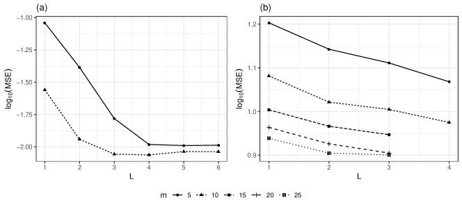
Figure 4: (a) Out-of-sample MSE (on $\log_{10}$ scale) attained by different models fitted on 1 dimensional heart-rate dataset with $m=5,10$ and $L=1,\ldots,6$.
(b) Out-of-sample MSE (on $\log_{10}$ scale) attained by different models fitted on 2 dimensional temperature dataset with $m=5,10,15,20,25$ and $L=1,\ldots,4$. For any $L>4$, our pruning algorithm 1 will reduce it to $L=4$; for $m=25$ our pruning algorithm will reduce SAGP model to $L=3$

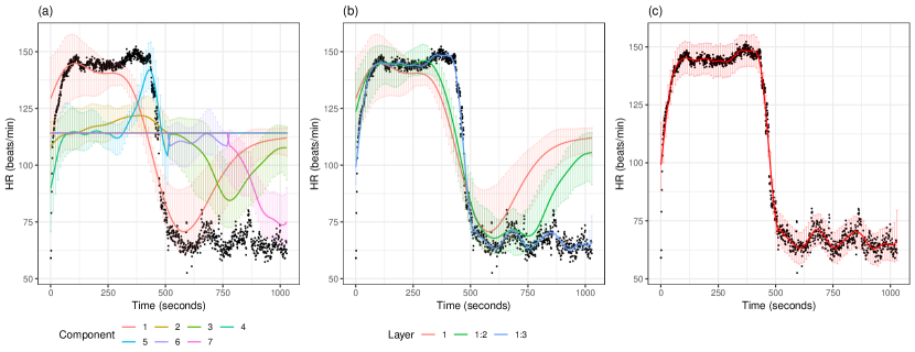
Figure 5: The panels show the observed HR values over time as black dots and results about the fit of the SAGP model with $m=10$ and $L=3$. Panel (a) shows the posterior means and the 95% CIs of the 7 additive components of the SAGP model on 100 equispaced locations on the support of the data. Panel (b) shows the posterior means and the 95% CIs of the sole component in layer 1 (red), of the components belonging to layer 1 and 2 (green) and of the complete model, including components from layer 1, 2 and 3. Panel (c) provides the predictive mean and the corresponding 95% prediction intervals.

5.2 Temperature Data

In this section we study a moderate sized 2-dimensional dataset of average daily maximum temperature in degrees centigrade at 247 locations in Colorado during 1997 US precipitation and temperature (1895-1997) dataset.

Qualitative comparisons of GP, BART and SAGP are shown in Figure 6. For GP regression we used MLE estimates with the $\mathsf{Matern}(5/2)$ kernel. For BART we use the default settings (Chipman et al., 2010). For SAGP, we choose $L=3,m=25$ and calibrate the $\alpha,\beta$ of the noise prior in SAGP and the noise estimate in BART according to MLE of noise estimate from GP. The GP model shows reasonable predictions, however, the prediction comes with high predictive variance in locations away from the observations and especially near the boundary (not shown). The predictive mean of BART shows it has a slight grid-like artifact due to its decision tree construction. In addition, the shape of the response around the mode is noticeably more rectangular than suggested by the other models.

This dataset provides us a 2-dimensional example where the data is limited, which is actually a disadvantage for SAGP since the sparsification does not cut down the computational cost significantly yet some information is lost in the procedure. Nonetheless, the SAGP method captures the major trends and even some of the extremal temperatures close to 40 degrees centigrade. Compared to BART and GP, the SAGP model behaves “in-between” these two methods and provides us with very competitive performance.

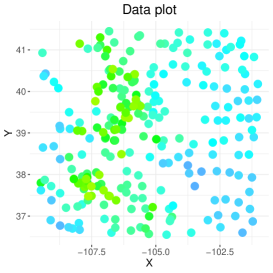
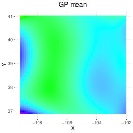
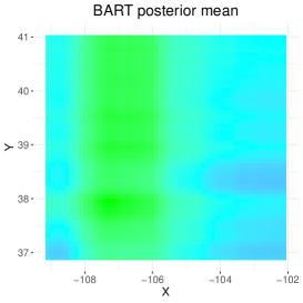
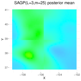
Figure 6: The original max temperature dataset for Colorado in 1997 summer. The horizontal axis is longitude; the vertical axis is latitude; the response is the observed values of maximal temperature in degrees Celsius. The typical raster plot for predictive means of Gaussian Process regression (Universal kriging with Gaussian kernel and MLE nuggets)/BART(number of trees $m=200$)/SAGP($m=25,L=3$) evaluated on a fine meshed grid (generated by steplengths of 0.1) on the original input domain.

5.3 Ice Sheet Data

The Ice Sheet data is a larger 2-dimensional dataset but this time with noticeably uneven sampling as discussed in Park and Apley (2018).The response is ice sheet thickness in meters collected over a region of west Antarctica (Blankenship et al., 2004).We used the data from 1991, first converting the longitude and latitude into 2-dimensional Euclidean coordinates and standardizing the dataset to $[0,1]^{2}$.

A plot of the data and predictive fits for the GP (exponential correlation), laGP, BART, treed GP (TGP; (Gramacy et al., 2007)) and SAGP models are shown in Figure 7. We included TGP in this plot as we thought it may be helpful with the unevenly sampled data but did not end up including it in our overall quantitative results below. For the SAGP model, we show the fit obtained with $L=3,m=10.$

The fits obtained among these models show quite different behaviors. The full GP fit possess extreme boundary behavior due to the lack of data near the boundary. The BART model shows more noticeable grid-like artifacts in this dataset, but does not suffer from the boundary effects seen with the GP. The TGP regression also does not exhibit boundary effects but has much higher variability of the mean response in the data-rich region which does not agree with the other models. The dynamic partitioning of TGP also introduces considerable computational cost. The laGP model with its default settings and MSPE criterion exhibits some degree of variability in the fitted mean response, particularly near the boundaries, however, it is the most computationally efficient method.

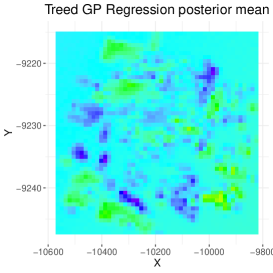
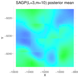
Figure 7: The scatter point plot shows the ice thickness in a region of Antarctica. The horizontal and the vertical axis are geographical coordinates in kilometers (km). The raster plot for predictive means of GP/laGP/BART(number of trees $m=200$)/TGP/SAGP($m=10,L=3$) for ice sheet dataset and evaluation on a fine meshed grid (generated by steplengths of 0.02) on the original input domain. The color scales and the axis are the same in these plots.

The SAGP model fit is reasonable. It does not have extreme values, high variability in the mean response or boundary effects like some of the other models, yet retains most of the smoothness suggested by the full GP fit.

5.4 United Kingdom Budget Data

This dataset is a well-known econometric dataset first studied in Blundell et al. (1998). The dataset consists of a cross-section of 1,519 households drawn from the 1980-1982 British Family Expenditure Surveys. We attempt to predict the total household expenditure (rounded to the nearest 10 UK pounds sterling) with 8 variables as inputs. We do not use the variable of the number of children per household in the regression, since the dataset is cleaned in such a way that it contains only households with one or two children, as presented in Blundell et al. (1998).

We choose this dataset to explore the performance of our SAGP model in the higher-dimensional scenario. As mentioned by Gramacy et al. (2016), such a dataset of high-dimensionality ($d=8$) will usually present computational challenges to classical GP models. Our main goal is to show that with reasonable increase of computational time, SAGP model has competitive performance. Since this dataset cannot be easily visualized, we only present quantitative results as shown in the next section.

5.5 Quantitative Performance Summary

The performance of SAGP and the alternative models considered is summarized quantitatively in Table 2. As in Section 4, we summarize the quantitative performance using 25% test set of original dataset to calculate out-of-sample RMSE, coverage of 95% credible intervals and interval scores. SAGP, SGP, GP, laGP, BART and BCART models were applied to all datasets. For SAGP, we generally selected $L=2\sim 4$ and $m=5\sim 15$ while for SGP we selected $m=5,15$ or $150.$ BART and BCART models were fit using their defaults, and laGP was fit using defaults but with both ALC and MSPE local design criteria.

Generally, we see that models could excel in one aspect (say RMSE) typically at the expense of another aspect of model fit quality, where the quality of fit depends on the dataset and application scenario. We notice that BART generally had lower coverage probability for the 95% PI and higher interval score. BCART had better coverage probability but generally was not the best in terms of RMSE. For the frequentist GP, two datasets exhibited good RMSE and two exhibited weaker RMSE performance. The GP is also less informative in terms of uncertainty quantification than the Bayesian models we considered. The laGP models often provided good RMSE performance, particularly with the ALC criterion, however the coverage was lower on the UK dataset.

In comparison, the SAGP model generally provided RMSE performance on par or near the best model for each dataset. The coverage also shows that SAGP models were consistent performers, especially compared to BART and laGP. We also see that SGP is uniformly worse than SAGP, often having either higher RMSE or worse coverage behavior. Overall, it is clear that SAGP is competitive with the best models for each dataset as summarized in Table 2, and we often prefer the qualitative aspect of the SAGP fits compared to some of the alternative models as demonstrated earlier.

6 Discussion

The SAGP model effectively borrows ideas from both sparsification and localization. In particular, we divide the input domain $\mathsf{X}$ in such a way that we can choose enough pseudo-inputs fit a sparse GP regression within the sub-region block of the partition, which also produces a trade-off for model parameters. We also showed that SAGP can achieve an effective reduction in computational cost (See Proposition 1) since all components within a layer can effectively be fit in parallel.

As a Bayesian additive model, SAGP provides uncertainty quantification and leads to refined posterior inference. Along the model building process, we also exhibit how the pseudo-inputs can be sampled to capture this aspect of model uncertainty, which is ignored with the fixed pseudo-inputs of SGP. The RP partition scheme outlined not only serves as a localization construction but also guarantees adequate pseudo-inputs for this resampling are available in each SAGP model component.As shown in the data analysis examples, the SAGP model is a competitive candidate compared to other generalization of GP regression methods. SAGP model can easily be generalized into higher dimensions, and our RP partition scheme is very flexible since it carries a hierarchical structure that allows us to analyze dataset in a multiscale way. With the homogeneous partition in one dimension, our RP scheme is similar to Bui and Turner (2014) and Lee et al. (2017); with heterogeneous partition in higher dimensions, our RP partition scheme is more flexible. For example, we can use binary partitioning in the first dimension but ternary partitioning in the second dimension. This will also preserve the hierarchical structure and allow us to decompose the high-dimensional data through different layers.

As for future works, there are various possible extensions of the proposed SAGP model. In terms of generalization of our current base model, we are interested in make the SAGP model admit different covariance kernels and different number of pseudo-inputs in each component. It is also of interest to extend the SAGP model to binary, count and categorical responses. To push the computational implementation of SAGP further and since independent sparse Gaussian process (SGP) regression model are fitted for each local component, it is readily seen that our model is parallelizable for efficient computation. Theoretically, we would also like to see a (frequentist) consistency result for SAGP model (Rocková and van der Pas, 2017) and a careful analysis of the effect of the choice of priors in this model.

Acknowledgments

The authors wish to thank the helpful feedback of the editor, associate editor and two anonymous reviewers, which helped to substantially improve the paper. The work of M.T.P. was supported in part by the National Science Foundation under Agreement DMS-1916231 and in part by the King Abdullah University of Science and Technology (KAUST) Office of Sponsored Research (OSR) under Award No. OSR-2018-CRG7-3800.3.

A Correlation between Targets as Function of the Distance between Inputs

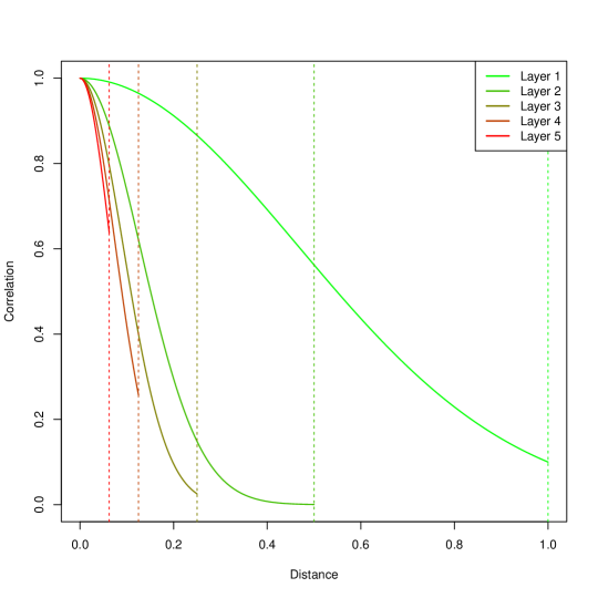
Figure 8: Given two one-dimensional inputs $\boldsymbol{x}_{i}$ and $\boldsymbol{x}_{i^{\prime}}$ ($d=1$), the figure represents the correlation between $f_{j}(\boldsymbol{x}_{i})$ and $f_{j}(\boldsymbol{x}_{i^{\prime}})$ (i.e., the targets of component $j$) as a function of the distance between $\boldsymbol{x}_{i}$ and $\boldsymbol{x}_{i^{\prime}}$. We represent with different colors the correlation that is assumed for components at different layers ($L=5$ in the Figure). Notably, the size of a component’s domain $B_{j}$ depends on the layer where the component is defined (the higher the layer index, the smaller the domain). Therefore, in our binary recursive partition scheme, the maximum possible distance between two inputs (highlighted with a vertical dashed line in the Figure) halves at each layer.

B Proof of Proposition 1

We first calculate the total number of components in the SAGP models when the input-domain is $[0,1]^{d}$. For each dimension $i=1,2,\ldots,d$, if we $b_{i}$-ary subdivide the $[0,1]$ interval, then there are at most $|\mathcal{L}_{\ell}|=\prod_{i=1}^{d}b_{i}^{\ell-1}$ individual components in form of $B(\boldsymbol{c}_{j},\boldsymbol{w}_{j})$ in the $\ell$-th layer of the RP scheme for $\ell=1,2,\ldots,L$.

For each component in the $\ell$-th layer, the number of observations fitted to the $j$-th component is at most $|\mathcal{X}^{(j)}|\leq n$. Then we fit a SGP model with $m$ pseudo-inputs, whose complexity is $\mathcal{O}(|\mathcal{X}^{(j)}|\cdot m^{2})$. Then for the $\ell$-th layer the total complexity is $\mathcal{O}(\sum_{B_{j}\in\mathcal{L}_{\ell}}|\mathcal{X}^{(j)}|\cdot m^{2})$. Therefore, for the $\ell$-th layer the complexity is at most $\mathcal{O}(|\mathcal{L}_{\ell}|\cdot n\cdot m^{2})$. Therefore we can compute the total complexity of the model as $\mathcal{O}(\sum_{\ell=1}^{L}|\mathcal{L}_{\ell}|\cdot n\cdot m^{2})\asymp\mathcal{O}\left(\sum_{\ell=1}^{L}\prod_{i=1}^{d}b_{i}^{\ell-1}\cdot n\cdot m^{2}\right)$.

C MCMC Algorithm for SAGP Model Fitting (Algorithm 3)

Algorithm 3 MCMC algorithm for SAGP model.

Input :

RP partition scheme consisting of $N$ components,   Number of pseudo-inputs for each component $m_{j}$,   Hyper-parameters for the prior of parameters,   Observed dataset $\{\mathcal{X},\boldsymbol{y}\}$.

Output :

Posterior samples for parameters, $\bar{\mathcal{X}}^{(j)},\bar{\boldsymbol{f}}_{j}$,   Predictive posterior samples for $\boldsymbol{y}_{*},\boldsymbol{f}_{j},\boldsymbol{y}$.

Initialization of the parameter values

while not converged do

2       Sample $\bar{\mathcal{X}}^{(j)},j=1,\ldots,N$ as in Algorithm 2. for $j$ in $1:N$ do

3             $\boldsymbol{r}_{j}\leftarrow\boldsymbol{y}-\sum_{l\neq j}\boldsymbol{K}_{nm_{l}}^{(l)}\left(\boldsymbol{K}_{m_{l}}^{(l)}\right)^{-1}\bar{\boldsymbol{f}}_{l}$  $\bar{\boldsymbol{f}}_{j}\leftarrow N_{m_{j}}(\boldsymbol{Mean}_{j},\boldsymbol{Var}_{j})$ as in (13)  $\eta_{j,\text{new}}\leftarrow\text{Uniform}(\eta_{j}\pm\text{bandwidth})$  $\alpha\leftarrow\min(1,{C\cdot\textnormal{{Model Likelihood}}(\eta_{j,new})}/{C\cdot\textnormal{{Model Likelihood}}(\eta_{j})})$  if Uniform(0,1)$\leq\alpha$ then

4                   $\eta_{j}\leftarrow\eta_{j,\text{new}}$

5             end if

6            // For every $\text{burn-in steps}/20$ steps, we adjust bandwidth. if $\text{Acceptance rate of }\eta_{j}\notin(0.39,0.49]$ then

7                   Band width for proposing $\eta_{j}\leftarrow\text{Acceptance rate of }\eta_{j}/0.44$  

8             end if

9            

10       end for

11      $\sigma_{\epsilon}^{2}\leftarrow\text{InverseGamma}\left(\alpha_{\epsilon}+\frac{n}{2},\beta_{\epsilon}+\frac{1}{2}(\boldsymbol{y}-\hat{\boldsymbol{y}})^{T}(\boldsymbol{y}-\hat{\boldsymbol{y}})\right)$ 

12 end while

D Detailed Derivation of Posterior Distribution in Section 3.2.5

To clarify our derivations, we first stated following simple lemma that will be used, which can be derived from Woodbury identity (Horn and Johnson, 1990) or a direct verification (Rasmussen and Williams, 2006).

Lemma 1

For a joint Gaussian distribution $\boldsymbol{a}\in\mathbb{R}^{n},\boldsymbol{b}\in\mathbb{R}^{n}$ if

$$\left(\begin{array}[]{c}\boldsymbol{a}\\ \boldsymbol{b}\end{array}\right) \propto N_{n+m}\left(\left(\begin{array}[]{c}\boldsymbol{\mu_{a}}\\ \boldsymbol{\mu_{b}}\end{array}\right),\left(\begin{array}[]{cc}C_{\boldsymbol{aa}}&C_{\boldsymbol{ab}}\\ C_{\boldsymbol{ba}}&C_{\boldsymbol{bb}}\end{array}\right)\right)$$ (21)

then its conditional distribution is:

$$\boldsymbol{a}\mid\boldsymbol{b} \sim N_{n}\left(\boldsymbol{\mu}_{\boldsymbol{a}}+C_{\boldsymbol{ab}}\left(C_{\boldsymbol{bb}}\right)^{-1}(\boldsymbol{b-\boldsymbol{\mu}_{b}}),C_{\boldsymbol{aa}}-C_{\boldsymbol{ab}}\left(C_{\boldsymbol{bb}}\right)^{-1}C_{\boldsymbol{ba}}\right)$$ (22)

In particular, for $f_{l}=f(\boldsymbol{x}_{l}),\bar{\boldsymbol{f}}_{j}=(\bar{f}_{j}(\bar{\boldsymbol{x}}_{1}),\ldots,\bar{f}_{j}(\bar{\boldsymbol{x}}_{m_{j}}))^{T}$ and covariance kernel function $K=K^{(j)},K_{ll}^{(j)}=K{}^{(j)}(\boldsymbol{x}_{l},\boldsymbol{x}_{l})$ if

$$\left.\left(\begin{array}[]{c}f_{l}\\ \bar{\boldsymbol{f}}_{j}\end{array}\right)\right|\bar{\mathcal{X}}^{(j)},\boldsymbol{x}_{l} \propto N_{1+m_{j}}\left(\left(\begin{array}[]{c}0\\ \boldsymbol{0}_{m_{j}}\end{array}\right),\left(\begin{array}[]{cc}K_{ll}^{(j)}&\boldsymbol{k}_{l}^{(j)T}\\ \boldsymbol{k}_{l}^{(j)}&\boldsymbol{K}_{m_{j}}^{(j)}\end{array}\right)\right)$$ (29)

then its conditional distribution is:

$$f_{l}\mid\bar{\boldsymbol{f}}_{j},\bar{\mathcal{X}}^{(j)},\boldsymbol{x}_{l} \sim N_{1}\left(\boldsymbol{k}_{l}^{(j)T}\left(\boldsymbol{K}_{m_{j}}^{(j)}\right)^{-1}\bar{\boldsymbol{f}}_{j},K_{ll}^{(j)}-\boldsymbol{k}_{l}^{(j)T}\left(\boldsymbol{K}_{m_{j}}^{(j)}\right)^{-1}\boldsymbol{k}_{l}^{(j)}\right)$$ (30)

We assume a Gaussian prior on the pseudo-targets as in (3.2.2).

$$P(\bar{\boldsymbol{f}}_{j}\mid\bar{\mathcal{X}}^{(j)}) \sim N_{m_{j}}\left(\bar{\boldsymbol{f}}_{j}\mid\boldsymbol{0}_{m_{j}},\boldsymbol{K}_{m_{j}}^{(j)}\right)$$ (31)

and then use Bayesian rule on the parameter $\bar{\boldsymbol{f}}_{j}$, recalling that (4) determines the form of mean and variance of the Gaussian distribution $P(\boldsymbol{y}\mid\bar{\boldsymbol{f}}_{1},\ldots,\bar{\boldsymbol{f}}_{N},\bar{\mathcal{X}}^{(1)},\ldots,\bar{\mathcal{X}}^{(N)},\mathcal{X},\boldsymbol{\boldsymbol{\kappa}})$.

$$P(\bar{\boldsymbol{f}}_{j}\mid\boldsymbol{y},\mathcal{X},\bar{\boldsymbol{f}}_{1},\ldots,\bar{\boldsymbol{f}}_{N},\bar{\mathcal{X}}^{(1)},\ldots,\bar{\mathcal{X}}^{(N)},\boldsymbol{\boldsymbol{\kappa}})$$

$$\propto P(\boldsymbol{y}\mid\bar{\boldsymbol{f}}_{1},\ldots\bar{\boldsymbol{f}}_{N},\bar{\mathcal{X}}^{(1)},\ldots,\bar{\mathcal{X}}^{(N)},\boldsymbol{\boldsymbol{\kappa}})\times$$

$$P(\bar{\boldsymbol{f}}_{j}\mid\{\boldsymbol{x}\}_{n},\bar{\boldsymbol{f}}_{1},\ldots,\bar{\boldsymbol{f}}_{j-1},\bar{\boldsymbol{f}}_{j+1},\ldots\bar{\boldsymbol{f}}_{N},\bar{\mathcal{X}}^{(1)},\ldots,\bar{\mathcal{X}}^{(N)},\boldsymbol{\boldsymbol{\kappa}})$$ (32)

$$= N_{n}\left(\left.\boldsymbol{y}-\sum_{l\neq j}\boldsymbol{K}_{nm_{l}}^{(l)}\left(\boldsymbol{K}_{m_{l}}^{(l)}\right)^{-1}\bar{\boldsymbol{f}}_{l}\right|\boldsymbol{K}_{nm_{j}}^{(j)}\left(\boldsymbol{K}_{m_{j}}^{(j)}\right)^{-1}\bar{\boldsymbol{f}}_{j},\boldsymbol{\Lambda}_{n}^{(j)}+\sigma_{\epsilon}^{2}\boldsymbol{I}_{n}\right)\times$$

$$N_{m_{j}}\left(\bar{\boldsymbol{f}}_{j}|\boldsymbol{0}_{m_{j}},\boldsymbol{K}_{m_{j}}^{(j)}\right)$$ (33)

We can derive the posterior using the normal normal conjugacy:

$$P(\bar{\boldsymbol{f}}_{j}\mid\boldsymbol{y},\mathcal{X},\bar{\boldsymbol{f}}_{1},\ldots,\bar{\boldsymbol{f}}_{j-1},\bar{\boldsymbol{f}}_{j+1},\ldots\bar{\boldsymbol{f}}_{N},\bar{\mathcal{X}}^{(1)},\ldots,\bar{\mathcal{X}}^{(N)},\boldsymbol{\boldsymbol{\kappa}})$$

$$\propto \frac{1}{\sqrt{\left|2\pi\left(\boldsymbol{\Lambda}_{n}^{(j)}+\sigma_{\epsilon}^{2}\boldsymbol{I}_{n}\right)\right|}}\exp\left\{-\frac{1}{2}\left[\boldsymbol{y}-\sum_{l=1}^{N}\boldsymbol{K}_{nm_{l}}^{(l)}\left(\boldsymbol{K}_{m_{l}}^{(l)}\right)^{-1}\bar{\boldsymbol{f}}_{l}\right]^{T}\left(\boldsymbol{\Lambda}_{n}^{(j)}+\sigma_{\epsilon}^{2}\boldsymbol{I}_{n}\right)^{-1}\times\right.$$

$$\left.\left[\boldsymbol{y}-\sum_{l=1}^{N}\boldsymbol{K}_{nm_{l}}^{(l)}\left(\boldsymbol{K}_{m_{l}}^{(l)}\right)^{-1}\bar{\boldsymbol{f}}_{l}\right]\right\}\times$$

$$\frac{1}{\sqrt{\left|2\pi\boldsymbol{K}_{m_{j}}\right|}}\exp\left\{-\frac{1}{2}\bar{\boldsymbol{f}}_{j}^{T}\boldsymbol{K}_{m_{j}}^{-1}\bar{\boldsymbol{f}}_{j}\right\}$$ (34)

We complete the squares inside the exponent,

$$\propto \exp\left\{-\frac{1}{2}\bar{\boldsymbol{f}}_{j}^{T}\left(\boldsymbol{K}_{m_{j}}^{-1}+\left[\left(\boldsymbol{K}_{m_{j}}^{(j)}\right)^{-1}\boldsymbol{K}_{m_{j}n}^{(j)}\left(\boldsymbol{\Lambda}_{n}^{(j)}+\sigma_{\epsilon}^{2}\boldsymbol{I}_{n}\right)^{-1}\boldsymbol{K}_{nm_{j}}^{(j)}\left(\boldsymbol{K}_{m_{j}}^{(j)}\right)^{-1}\right]\right)\bar{\boldsymbol{f}}_{j}\right.$$

$$\left.-\boldsymbol{f}_{j}^{T}\left(\boldsymbol{\Lambda}_{n}^{(j)}+\sigma_{\epsilon}^{2}\boldsymbol{I}_{n}\right)^{-1}\boldsymbol{K}_{nm_{j}}^{(j)}\left(\boldsymbol{K}_{m_{j}}^{(j)}\right)^{-1}\bar{\boldsymbol{f}}_{j}+\text{proportionally constant terms}\right\}$$ (35)

After completing square we can obtain the mean and variance of the $j$-th component:

$$\boldsymbol{Mean}_{j}= \left(\left(\boldsymbol{K}_{m_{j}}^{(j)}\right)^{-1}+\left[\left(\boldsymbol{K}_{m_{j}}^{(j)}\right)^{-1}\boldsymbol{K}_{m_{j}n}^{(j)}\left(\boldsymbol{\Lambda}_{n}^{(j)}+\sigma_{\epsilon}^{2}\boldsymbol{I}_{n}\right)^{-1}\boldsymbol{K}_{nm_{j}}^{(j)}\left(\boldsymbol{K}_{m_{j}}^{(j)}\right)^{-1}\right]\right)\times$$

$$\left(\left(\boldsymbol{y}-\sum_{l\neq j}\boldsymbol{K}_{nm_{l}}^{(l)}\left(\boldsymbol{K}_{m_{l}}^{(l)}\right)^{-1}\bar{\boldsymbol{f}}_{l}\right)^{T}\left(\boldsymbol{\Lambda}_{n}^{(j)}+\sigma_{\epsilon}^{2}\boldsymbol{I}_{n}\right)^{-1}\boldsymbol{K}_{nm_{j}}^{(j)}\left(\boldsymbol{K}_{m_{j}}^{(j)}\right)^{-1}\right)^{T}$$

$$= \boldsymbol{K}_{m_{j}}^{(j)}\boldsymbol{Q}_{m_{j}}^{(j)-1}\boldsymbol{K}_{m_{j}n}^{(j)}\left(\boldsymbol{\Lambda}_{n}^{(j)}+\sigma_{\epsilon}^{2}\boldsymbol{I}_{n}\right)^{-1}\left(\boldsymbol{y}-\sum_{l\neq j}\boldsymbol{K}_{nm_{l}}^{(l)}\left(\boldsymbol{K}_{m_{l}}^{(l)}\right)^{-1}\bar{\boldsymbol{f}}_{l}\right)$$ (36)

By Woodbury identity, we know that for $\boldsymbol{Q}_{m_{j}}^{(j)}=\boldsymbol{K}_{m_{j}}^{(j)}+\boldsymbol{K}_{m_{j}n}^{(j)}\left(\boldsymbol{\Lambda}_{n}^{(j)}+\sigma_{\epsilon}^{2}\boldsymbol{I}_{n}\right)^{-1}\boldsymbol{K}_{nm_{j}}^{(j)}$ we can write its inverse as

$$\boldsymbol{Q}_{m_{j}}^{(j)-1} =\left\{\boldsymbol{K}_{m_{j}}^{(j)-1}-\boldsymbol{K}_{m_{j}}^{(j)-1}\boldsymbol{K}_{m_{j}n}^{(j)}\left[\left(\boldsymbol{\Lambda}_{n}^{(j)}+\sigma_{\epsilon}^{2}\boldsymbol{I}_{n}\right)+\boldsymbol{K}_{nm_{j}}^{(j)}\boldsymbol{K}_{m_{j}}^{(j)-1}\boldsymbol{K}_{m_{j}n}^{(j)}\right]^{-1}\boldsymbol{K}_{nm_{j}}^{(j)}\boldsymbol{K}_{m_{j}}^{(j)-1}\right\}$$

Using this $m_{j}\times m_{j}$ matrix $\boldsymbol{Q}_{m_{j}}$, we can write down the covariance matrix $\boldsymbol{Var}_{j}$:

$$\boldsymbol{Var}_{j}= \left(\left(\boldsymbol{K}_{m_{j}}^{(j)}\right)^{-1}+\left[\left(\boldsymbol{K}_{m_{j}}^{(j)}\right)^{-1}\boldsymbol{K}_{m_{j}n}^{(j)}\left(\boldsymbol{\Lambda}_{n}^{(j)}+\sigma_{\epsilon}^{2}\boldsymbol{I}_{n}\right)^{-1}\boldsymbol{K}_{nm_{j}}^{(j)}\left(\boldsymbol{K}_{m_{j}}^{(j)}\right)^{-1}\right]\right)^{-1}$$ (37)

$$= \boldsymbol{K}_{m_{j}}^{(j)}-\boldsymbol{K}_{m_{j}}^{(j)}\left[\left(\boldsymbol{K}_{m_{j}}^{(j)}\right)^{-1}\boldsymbol{K}_{m_{j}n}^{(j)}\right]\times$$

$$\left[\left(\boldsymbol{\Lambda}_{n}^{(j)}+\sigma_{\epsilon}^{2}\boldsymbol{I}_{n}\right)+\boldsymbol{K}_{nm_{j}}^{(j)}\left(\boldsymbol{K}_{m_{j}}^{(j)}\right)^{-1}\boldsymbol{K}_{m_{j}}^{(j)}\left(\boldsymbol{K}_{m_{j}}^{(j)}\right)^{-1}\boldsymbol{K}_{m_{j}n}^{(j)}\right]^{-1}\times$$

$$\boldsymbol{K}_{nm_{j}}^{(j)}\left(\boldsymbol{K}_{m_{j}}^{(j)}\right)^{-1}\boldsymbol{K}_{m_{j}}^{(j)}$$ (38)

$$= \boldsymbol{K}_{m_{j}}^{(j)}-\boldsymbol{K}_{m_{j}n}^{(j)}\left[\left(\boldsymbol{\Lambda}_{n}^{(j)}+\sigma_{\epsilon}^{2}\boldsymbol{I}_{n}\right)+\boldsymbol{K}_{nm_{j}}^{(j)}\left(\boldsymbol{K}_{m_{j}}^{(j)}\right)^{-1}\boldsymbol{K}_{m_{j}n}^{(j)}\right]^{-1}\boldsymbol{K}_{nm_{j}}^{(j)}$$

$$= \boldsymbol{K}_{m_{j}}^{(j)}\left\{\left(\boldsymbol{K}_{m_{j}}^{(j)}\right)^{-1}-\right.$$

$$\left.\left(\boldsymbol{K}_{m_{j}}^{(j)}\right)^{-1}\boldsymbol{K}_{m_{j}n}^{(j)}\left[\left(\boldsymbol{\Lambda}_{n}^{(j)}+\sigma_{\epsilon}^{2}\boldsymbol{I}_{n}\right)+\boldsymbol{K}_{nm_{j}}^{(j)}\left(\boldsymbol{K}_{m_{j}}^{(j)}\right)^{-1}\boldsymbol{K}_{m_{j}n}^{(j)}\right]^{-1}\left(\boldsymbol{K}_{m_{j}}^{(j)}\right)^{-1}\right\}\boldsymbol{K}_{nm_{j}}^{(j)}$$ (39)

$$= \boldsymbol{K}_{m_{j}}^{(j)}\boldsymbol{Q}_{m_{j}}^{(j)-1}\boldsymbol{K}_{m_{j}}^{(j)}$$ (40)

Note that although we do need to invert an $n\times n$ matrix $\boldsymbol{\Lambda}_{n}^{(j)}+\sigma_{\epsilon}^{2}\boldsymbol{I}_{n}$, it is a diagonal matrix and hence easy to invert as claimed before.

E Diagnostic Statistics for the SAGP Model on 1000 Batches of Simulated Dataset

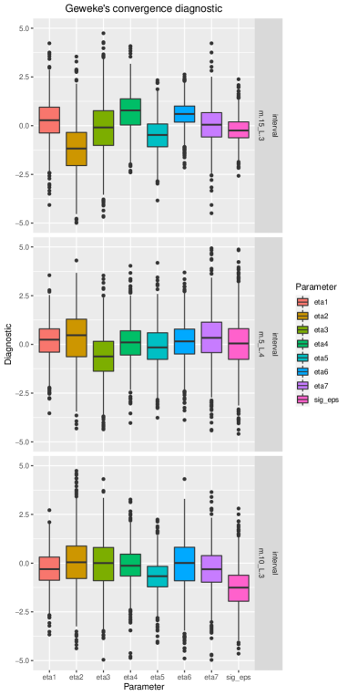
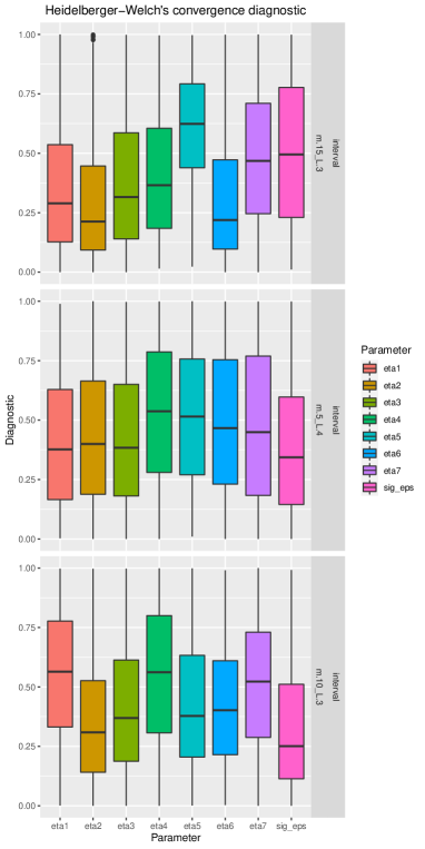
Figure 9: The panels of box plots show the Geweke’s convergence diagnostic (Geweke et al., 1991) and Heidelberger-Welch’s convergence diagnostic (Heidelberger and Welch, 1983) based on the MCMC sample of SAGP model, for parameter $\eta^{(j)}$ and $\sigma_{\epsilon}^{2}$, calculated from the 1000 batches of simulated dataset from formula (14) with the testing set is random or interval.

F Heart Rate Dataset Analyzed by SAGP Model Fitted with $m=5$ and $L=4$ (Figure 10)

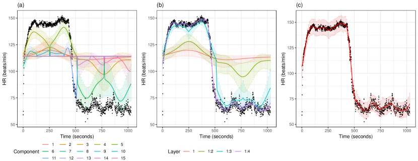
Figure 10: The panels show the observed HR values over time as black dots and results about the fit of the SAGP model with $m=5$ and $L=4$. Panel (a) shows the posterior means and the 95% CIs of the 15 additive components of the SAGP model on 100 equispaced locations on the support of the data. Panel (b) shows the posterior means and the 95% CIs of the sole component in layer 1 (red), of the components belonging to layer 1 and 2 (green) , of the components belonging to layer 1, 2, 3 and of the complete model, including components from layer 1, 2, 3 and 4. Panel (c) provides the predictive mean and the corresponding 95% prediction intervals.

References

- Alan E. Gelfand (1990) Amy Racine-Poon & Adrian F. M. Smith Alan E. Gelfand, Susan E. Hills. Illustration of bayesian inference in normal data models using gibbs sampling. Journal of the American Statistical Association, 85.412:972–985, 1990.
- Banerjee et al. (2012) Anjishnu Banerjee, David B. Dunson, and Surya T. Tokdar. Efficient gaussian process regression for large datasets. Biometrika, 100.1:75–89, 2012.
- Blankenship et al. (2004) D. D. Blankenship et al. Ice thickness and surface elevation, southeastern ross embayment, west antarctica. U.S. Antarctic Program (USAP) Data Center, 2004. doi: doi:10.7265/N5WW7FKC. URL https://www.usap-dc.org/view/dataset/609099.
- Blundell et al. (1998) Richard Blundell, Alan Duncan, and Krishna Pendakur. Semiparametric estimation and consumer demand. Journal of applied econometrics, 13(5):435–461, 1998.
- Breiman (1984) Leo Breiman. Classification and Regression Trees. Belmont, California: Wadsworth, 1984.
- Bui and Turner (2014) Thang D. Bui and Richard E. Turner. Tree-structured gaussian process approximations. In Advances in Neural Information Processing Systems, 2014.
- Chipman et al. (1998) Hugh A. Chipman, Edward I. George, and Robert E. McCulloch. Bayesian cart model search. Journal of the American Statistical Association, 93.443:935–948, 1998.
- Chipman et al. (2010) Hugh A. Chipman, Edward I. George, and Robert E. McCulloch. Bart: Bayesian additive regression trees. The Annals of Applied Statistics, 4.1:266–298, 2010.
- Chipman et al. (2016) Hugh A. Chipman et al. High-dimensional nonparametric monotone function estimation using bart. arXiv preprint arXiv:1612.01619, 2016.
- Damianou and Lawrence (2013) Andreas Damianou and Neil D. Lawrence. Deep gaussian processes. Artificial Intelligence and Statistics, 2013.
- Denison et al. (1998) David G.T. Denison, Bani K. Mallick, and Adrian F.M. Smith. A bayesian cart algorithm. Biometrika, 85.2:363–377, 1998.
- Fox and Dunson (2012) Emily Fox and David B. Dunson. Multiresolution gaussian processes. Advances in Neural Information Processing Systems, 2012.
- Gelman et al. (2013) Andrew Gelman et al. Bayesian Data Analysis. New York : CRC Press : Taylor & Francis Group, 2013.
- Geweke et al. (1991) John Geweke et al. Evaluating the accuracy of sampling-based approaches to the calculation of posterior moments, volume 196. Federal Reserve Bank of Minneapolis, Research Department Minneapolis, MN, 1991.
- Gneiting and Raftery (2007) Tilmann Gneiting and Adrian E. Raftery. Strictly proper scoring rules, prediction, and estimation. Journal of the American Statistical Association, 102.477:359–378, 2007.
- Gramacy and Apley (2015) Robert B. Gramacy and Daniel W. Apley. Local gaussian process approximation for large computer experiments. Journal of Computational and Graphical Statistics, 24.2:561–578, 2015.
- Gramacy et al. (2007) Robert B. Gramacy et al. tgp: an r package for bayesian nonstationary, semiparametric nonlinear regression and design by treed gaussian process models. Journal of Statistical Software, 19.9:1–46, 2007.
- Gramacy et al. (2016) Robert B. Gramacy et al. lagp: large-scale spatial modeling via local approximate gaussian processes in r. Journal of Statistical Software, 72.1:1–46, 2016.
- Hastie and Tibshirani (1990) Trevor J. Hastie and Robert J. Tibshirani. Generalized Additive Models. New York : Chapman and Hall, 1990.
- Hastie and Tibshirani (2000) Trevor J. Hastie and Robert J. Tibshirani. Bayesian backfitting (with comments and a rejoinder by the authors. Statistical Science, 15.3:196–223, 2000.
- Heidelberger and Welch (1983) Philip Heidelberger and Peter D. Welch. Simulation run length control in the presence of an initial transient. Operations Research, 31.6:1109–1144, 1983.
- Horn and Johnson (1990) Roger A. Horn and Charles R. Johnson. Matrix Analysis. Cambridge: Cambridge university press, 1990.
- Kaufman et al. (2008) Cari G. Kaufman, Mark J. Schervish, and Douglas W. Nychka. Covariance tapering for likelihood-based estimation in large spatial data sets. Journal of the American Statistical Association, 103.484:1545–1555, 2008.
- Lawrence et al. (2003) Neil D. Lawrence, Ralf Herbrich, and Matthias Seeger. Fast sparse gaussian process methods: The informative vector machine. In Advances in neural information processing systems, 2003.
- Lee et al. (2017) Byung-Jun Lee, Jongmin Lee, and Kee-Eung Kim. Hierarchically-partitioned gaussian process approximation. In Artificial Intelligence and Statistics, 2017.
- Liu et al. (2018) Haitao Liu et al. When gaussian process meets big data: A review of scalable gps. arXiv preprint arXiv:1807.01065, 2018.
- Nguyen-Tuong et al. (2009) Duy Nguyen-Tuong, Matthias Seeger, and Jan Peters. Model learning with local gaussian process regression. Advanced Robotics, 23.15:2015–2034, 2009.
- Park and Apley (2018) Chiwoo Park and Daniel Apley. Patchwork kriging for large-scale gaussian process regression. The Journal of Machine Learning Research, 19.1:269–311, 2018.
- Park and Huang (2016) Chiwoo Park and Jianhua Z. Huang. Efficient computation of gaussian process regression for large spatial data sets by patching local gaussian processes. Journal of Machine Learning Research, 17.174:1–29, 2016.
- Pratola et al. (2019) Matthew T. Pratola, C Devon Lin, and Peter F. Craigmile. Optimal design emulators: A point process approach. arXiv preprint arXiv:1804.02089, 2019.
- Pratola et al. (2018) Matthew T. Pratola et al. Heteroscedastic bart using multiplicative regression trees. arXiv preprint arXiv:1709.07542, 2018.
- Quinonero-Candela and Rasmussen (2005) Joaquin Quinonero-Candela and Carl E. Rasmussen. A unifying view of sparse approximate gaussian process regression. Journal of Machine Learning Research, 6:1939–1959, 2005.
- Rasmussen and Williams (2006) Carl E. Rasmussen and Christopher K.I. Williams. Gaussian Process for Machine Learning. Cambridge: MIT press, 2006.
- Rocková and van der Pas (2017) Veronika Rocková and Stéphanie van der Pas. Posterior concentration for bayesian regression trees and forests. arXiv preprint arXiv:1708.08734, 2017.
- Roustant et al. (2012) Olivier Roustant, David Ginsbourger, and Yves Deville. Dicekriging, diceoptim: Two r packages for the analysis of computer experiments by kriging-based metamodeling and optimization. Journal of Statistical Software, Articles, 51.1, 2012.
- Snelson and Ghahramani (2006) Edward Snelson and Zoubin Ghahramani. Sparse gaussian processes using pseudo-inputs. In Advances in neural information processing systems, 2006.
- Snelson and Ghahramani (2007) Edward Snelson and Zoubin Ghahramani. Local and global sparse gaussian process approximations. In Artificial Intelligence and Statistics, 2007.
- Storer (2012) James Andrew Storer. An Introduction to Data structures and Algorithms. New York : Springer, 2012.
- Titsias (2009) Michali Titsias. Variational learning of inducing variables in sparse gaussian processes. Artificial Intelligence and Statistics, 2009.
- Zakynthinaki (2015) Maria S. Zakynthinaki. Modelling heart rate kinetics. PloS one, 10.4, 2015.