Gaussian implementation of the multi-Bernoulli mixture filter

Abstract

This paper presents the Gaussian implementation of the multi-Bernoulli mixture (MBM) filter. The MBM filter provides the filtering (multi-target) density for the standard dynamic and radar measurement models when the birth model is multi-Bernoulli or multi-Bernoulli mixture. Under linear/Gaussian models, the single target densities of the MBM mixture admit Gaussian closed-form expressions. Murty’s algorithm is used to select the global hypotheses with highest weights. The MBM filter is compared with other algorithms in the literature via numerical simulations.

I Introduction

Multiple target tracking (MTT) is an important problem in many applications, such as, surveillance, autonomous vehicles and air traffic control [1, 2]. Relevant MTT algorithms are multiple hypothesis tracking [3, 4, 5, 6], joint probabilistic data association [7], and algorithms based on random finite sets (RFSs) [8].

In the RFS formulation, the (multi-target) filtering density contains the information of the target states at the current time step. This density can be used to estimate the number of current targets and their current states, which is a sub-problem of MTT referred to as multi-target filtering. For the standard (point target) dynamic and measurement models [8], there are multi-target conjugate prior densities that can be used to compute or approximate the filtering density. Multi-target conjugacy refers to a family of multi-target distributions which is closed under both the prediction and update steps [9, 10, 11]. We usually consider multi-target conjugate prior mixtures in which the number of components grows with time.

The Poisson multi-Bernoulli mixture (PMBM) [10] is a multi-target conjugate prior that can be written in terms of single target densities. If the birth model is a Poisson RFS, the filtering density is a PMBM. In this case, the Poisson part represents the targets that have never been detected and each component of the mixture is a global hypothesis, which has a certain weight and an associated multi-Bernoulli density.

A special case of a PMBM is a multi-Bernoulli mixture (MBM), which is obtained by setting the intensity of the Poisson RFS to zero in a PMBM. The MBM is a multi-target conjugate prior for the standard models if the birth process is multi-Bernoulli or MBM [11, Corollary 3]. The resulting filter is referred to as to the MBM filter, which is similar to the PMBM filter, but with a different processing of new born targets. Another multi-target conjugate prior is an MBM in which the existence probabilities of all Bernoulli components are either 0 or 1 (MBM₀₁). Given any MBM with probabilities of existence between 0 and 1, it can be parameterised in MBM₀₁ form, but with an exponential increase in the number of mixture components [11]. The $\delta$-generalised labelled multi-Bernoulli ($\delta$-GLMB) density [9] is a multi-target conjugate prior that is similar in structure to an MBM₀₁ in which targets (Bernoulli components) are uniquely labelled [11, Sec. IV].

The main contribution of this paper is to provide a thorough description of the MBM filter and its Gaussian implementation for linear and Gaussian models. In the proposed implementation, we make use of Murty’s algorithm [12] to prune the global hypotheses, which is a common approach in MTT [13, 14, 9]. We also indicate that the MBM filter can be labelled to provide a labelled MBM filter, which has the same filtering recursion as the MBM filter. We show simulation results comparing the MBM filter with the PMBM and MBM₀₁ filters.

The rest of the paper is organised as follows. In Section II, we formulate the problem and introduce the relevant conjugate priors. In Section III, we describe the MBM filter. Section IV addresses the proposed Gaussian implementation. Simulation results are shown in Section V. Finally, conclusions are drawn in Section VI.

II Problem formulation

In this section, we describe the standard dynamic model, with Poisson and multi-Bernoulli birth, and the standard measurement model. We also explain the multi-target conjugate priors.

The set of targets at time step $k$ is denoted as $X_{k}\in\mathcal{F}\left(\mathcal{X}\right)$, where $\mathcal{X}$ is the single target space, often $\mathcal{X}=\mathbb{R}^{n_{x}}$, and $\mathcal{F}\left(\mathcal{X}\right)$ is the the space of all finite subsets of $\mathcal{X}$. Given $X_{k}$, each target $x\in X_{k}$ survives to time step $k+1$ with probability $p_{S}\left(x\right)$ and moves to a new state with a transition density $g\left(\cdot\left|x\right.\right)$, or dies with probability $1-p_{S}\left(x\right)$. Set $X_{k+1}$ is then the union of the surviving targets and new targets, which are born independently of the rest.

We consider two types of birth model: a Poisson RFS, which is also called Poisson point process, with intensity $\lambda_{k}^{b}\left(\cdot\right)$, and a multi-Bernoulli RFS, which has $n_{k}^{b}$ Bernoulli components and the $l$-th Bernoulli component has existence probability $r_{k}^{b,l}$ and single target density $p_{k}^{b,l}\left(\cdot\right)$. The corresponding density is [11]

$$f_{k}^{b}\left(X_{k}\right) =\sum_{X^{1}\uplus...\uplus X^{n_{k}^{b}}=X_{k}}\prod_{l=1}^{n_{k}^{b}}f_{k}^{b,l}\left(X^{l}\right)$$ (1)

where $\uplus$ denotes the disjoint union and the density of the $l$-th Bernoulli component is

$$f_{k}^{b,l}\left(X_{k}\right)=\begin{cases}1-r_{k}^{b,l}&X_{k}=\emptyset\\ r_{k}^{b,l}p_{k}^{b,l}\left(x\right)&X_{k}=\left\{x\right\}\\ 0&\mathrm{otherwise}.\end{cases}$$ (2)

Note that in (1) the summation is taken over all mutually disjoint (and possibly empty) sets $X^{1},...,X^{n_{k}^{b}}$ whose union is $X_{k}$.

At time step $k$, we observe $X_{k}$ by a set $Z_{k}=\left\{z_{k}^{1},...,z_{k}^{m_{k}}\right\}\in\mathcal{F}\left(\mathbb{R}^{n_{z}}\right)$ of measurements. Given $X_{k}$, each target state $x\in X_{k}$ is either detected with probability $p_{D}\left(x\right)$ and generates one measurement with density $l\left(\cdot|x\right)$, or missed with probability $1-p_{D}\left(x\right)$. The set $Z_{k}$ is the union of the target-generated measurements and Poisson clutter with intensity $\kappa\left(\cdot\right)$.

In multi-target filtering, the objective is to compute the density of $X_{k}$ given the sequence of measurements $\left(Z_{1},...,Z_{k}\right)$. This density can be computed recursively by the prediction and the update steps of the filtering recursion [8]. This computation is aided by the use of multi-target conjugate priors

II-A Multi-target conjugate priors

We first explain the PMBM conjugate prior [10]. A PMBM is the density of the union of two independent RFS: a Poisson RFS with density $f^{p}\left(\cdot\right)$, and a multi-Bernoulli mixture RFS with density $f^{mbm}\left(\cdot\right)$. Then, the PMBM density is [10]

$$f\left(X\right) =\sum_{Y\uplus W=X}f^{p}\left(Y\right)f^{mbm}\left(W\right)$$

$$f^{p}\left(X\right) =e^{-\int\lambda\left(x\right)dx}\left[\lambda\left(\cdot\right)\right]^{X}$$

$$f^{mbm}\left(X\right) \propto\sum_{j}\sum_{X^{1}\uplus...\uplus X^{n}=X}\prod_{i=1}^{n}\left[w^{i,j}f^{i,j}\left(X^{i}\right)\right]$$

where $\lambda\left(\cdot\right)$ is the intensity of the Poisson RFS, $\propto$ stands for “proportional to”, $j$ is an index that goes through all the mixture components (also called global hypotheses), $f^{i,j}\left(\cdot\right)$ is the $i$-th Bernoulli RFS in the $j$-th global hypothesis, and $w^{i,j}$ its weight. It should be noted that the weight $w^{j}$ of the $j$-th global hypothesis is

$$w^{j} \propto\prod_{i=1}^{n}w^{i,j}.$$

A particular, relevant case of the PMBM is the multi-Bernoulli mixture (MBM), which is obtained by setting $\lambda\left(\cdot\right)=0$.

It is shown in [10] that, for the Poisson birth model, the filtering and predicted density are PMBM, which gives rise to the PMBM filter. A corollary of this fundamental result is that the MBM is conjugate prior if the birth model is multi-Bernoulli or MBM [11, Corollary 3]. In this work, we describe the MBM filter only for multi-Bernoulli birth model as the prediction step is simpler than for MBM birth [11]. We proceed to describe this filter in the next section.

III Multi-Bernoulli mixture filter

The density of $X_{k^{\prime}}$ with $k^{\prime}\in\left\{k,k+1\right\}$ given the measurements up to time step $k$ is an MBM with the form

$$f_{k^{\prime}|k}\left(X_{k^{\prime}}\right) \propto\sum_{a\in\mathcal{A}_{k^{\prime}|k}}\sum_{\uplus_{l=1}^{n_{k^{\prime}|k}}X^{l}=X_{k^{\prime}}}\prod_{i=1}^{n_{k^{\prime}|k}}\left[w_{k^{\prime}|k}^{i,a^{i}}f_{k^{\prime}|k}^{i,a^{i}}\left(X^{i}\right)\right].$$ (3)

We proceed to explain Equation (3). First, $n_{k^{\prime}|k}$ is the number of Bernoulli components, $i$ is an index over the Bernoulli components and a global hypothesis $a=\left(a^{1},...,a^{n_{k^{\prime}|k}}\right)$ contains the single target hypotheses for all Bernoulli components. The single target hypothesis for the $i$-th Bernoulli component is $a^{i}=\left(t^{i},l^{i},\xi_{t^{i}:k}^{i}\right)$ where $t^{i}$ and $l^{i}$ are its birth time and birth index, see (1), and $\xi_{t^{i}:k}^{i}=\left(\xi_{t^{i}}^{i},...,\xi_{k}^{i}\right)$ contains the corresponding data associations up to time step $k$. In this paper, we write $\xi_{j}^{i}=0$ if the $i$-th Bernoulli component has been misdetected at time step $j$ and $\xi_{j}^{i}=p\in\left\{1,...,m_{k}\right\}$ if the $i$-th Bernoulli component has been associated to the $p$-th measurement at time step $j$. Note that, for new born Bernoulli components, the single target hypothesis in the predicted density is only the pair $a^{i}=\left(t^{i},l^{i}\right)$, as there has not been a data association event for this component yet.

In each global hypothesis $a$, a measurement $z_{k}^{j}$ can only be assigned to one Bernoulli component, born at time step $k$ or before, and a Bernoulli component can be assigned at most to one measurement at each time step. All possible global hypotheses constitute the set of global hypotheses $\mathcal{A}_{k^{\prime}|k}$. Measurements left unassigned in a global hypothesis are considered clutter under this global hypothesis. Bernoulli components left unassigned at a particular time step in a global hypothesis are considered misdetected.

The density $f_{k^{\prime}|k}^{i,a^{i}}\left(\cdot\right)$ of the $i$-th Bernoulli component with single target hypothesis $a^{i}$ is written as

$$f_{k^{\prime}|k}^{i,a^{i}}\left(X\right) =\begin{cases}1-r_{k^{\prime}|k}^{i,a^{i}}&X=\emptyset\\ r_{k^{\prime}|k}^{i,a^{i}}p_{k^{\prime}|k}^{i,a^{i}}\left(x\right)&X=\left\{x\right\}\\ 0&\mathrm{otherwise}\end{cases}$$ (4)

and has an associated weight $w_{k^{\prime}|k}^{i,a^{i}}$.

In the rest of this section, we explain the prediction and update steps to recursively compute (3) in Sections III-A and III-B. A discussion of the recursion is given in Section III-C. We will use the following notation for the inner product of two functions $h\left(\cdot\right)$ and $g\left(\cdot\right)$

$$\left\langle h,g\right\rangle =\int h\left(x\right)g\left(x\right)dx.$$

III-A Prediction

We consider that the filtering density at time step $k$ is an MBM of the form (3) with $k^{\prime}=k$. Then, the predicted density has the same number of global hypotheses as the filtering density but with $n_{k+1|k}=n_{k|k}+n_{k+1}^{b}$ Bernoulli components. That is, each global hypothesis is augmented with the Bernoulli components that represent new born targets. For the surviving Bernoulli components, $i\in\left\{1,...,n_{k|k}\right\}$, the parameters are

$$w_{k+1|k}^{i,a^{i}} =w_{k|k}^{i,a^{i}}$$ (5)

$$r_{k+1|k}^{i,a^{i}} =r_{k|k}^{i,a^{i}}\left\langle p_{S},p_{k|k}^{i,a^{i}}\right\rangle$$ (6)

$$p_{k+1|k}^{i,a^{i}}\left(x\right) =\frac{\int g\left(x\left|y\right.\right)p_{S}\left(y\right)p_{k|k}^{i,a^{i}}\left(y\right)dy}{\left\langle p_{k|k}^{i,a^{i}},p_{S}\right\rangle}.$$ (7)

For Bernoulli components of new born targets, $i\in\left\{n_{k|k}+1,...,n_{k+1|k}\right\}$, the parameters are

$$a^{i} =\left(k+1,i-n_{k|k}\right)$$ (8)

$$w_{k+1|k}^{i,a^{i}} =1$$ (9)

$$r_{k+1|k}^{i,a^{i}} =r_{k+1}^{b,i-n_{k|k}}$$ (10)

$$p_{k+1|k}^{i,a^{i}}\left(x\right) =p_{k+1}^{b,i-n_{k|k}}\left(x\right).$$ (11)

III-B Update

We recall that the set of measurements at time step $k$ is denoted as $Z_{k}=\left\{z_{k}^{1},...,z_{k}^{m_{k}}\right\}$. The number of Bernoulli components does not change in the update so $n_{k|k}=n_{k|k-1}$. The update of the $i$-th Bernoulli component is as follows. We go through all single target hypotheses and create misdetection and measurement associated hypotheses. In this section, we use $\left(a^{i},p\right)$, with $p\in\left\{0,...,m_{k}\right\}$ to append $p$ to the single target hypothesis $a^{i}$. For a single target hypothesis $a^{i}$ at the previous time step, the misdetection single target hypothesis is characterised by

$$w_{k|k}^{i,\left(a^{i},0\right)} =w_{k|k-1}^{i,a^{i}}$$

$$\,\times\left(1-r_{k|k-1}^{i,a^{i}}+r_{k|k-1}^{i,a^{i}}\left\langle p_{k|k-1}^{i,a^{i}},1-p_{D}\right\rangle\right)$$ (12)

$$r_{k|k}^{i,\left(a^{i},0\right)} =\frac{r_{k|k-1}^{i,a^{i}}\left\langle p_{k|k-1}^{i,a^{i}},1-p_{D}\right\rangle}{1-r_{k|k-1}^{i,a^{i}}+r_{k|k-1}^{i,a^{i}}\left\langle p_{k|k-1}^{i,a^{i}},1-p_{D}\right\rangle}$$ (13)

$$p_{k|k}^{i,\left(a^{i},0\right)}\left(x\right) =\frac{\left(1-p_{D}\left(x\right)\right)p_{k|k-1}^{i,a^{i}}\left(x\right)}{\left\langle p_{k|k-1}^{i,a^{i}},1-p_{D}\right\rangle}.$$ (14)

The corresponding updated single target hypothesis with measurement $z_{k}^{j}$ is characterised by

$$w_{k|k}^{i,\left(a^{i},j\right)} =\frac{w_{k|k-1}^{i,a^{i}}r_{k|k-1}^{i,a^{i}}\left\langle p_{k|k-1}^{i,a^{i}},p_{D}l\left(z_{k}^{j}|\cdot\right)\right\rangle}{\kappa\left(z_{k}^{j}\right)}$$ (15)

$$r_{k|k}^{i,\left(a^{i},j\right)} =1$$ (16)

$$p_{k|k}^{i,\left(a^{i},j\right)}\left(x\right) =\frac{p_{D}\left(x\right)l\left(z_{k}^{j}|x\right)p_{k|k-1}^{i,a^{i}}\left(x\right)}{\left\langle p_{k|k-1}^{i,a^{i}},p_{D}l\left(z_{k}^{j}|\cdot\right)\right\rangle}.$$ (17)

Once we have formed the single target hypotheses for all Bernoulli components, a previous global hypothesis generates new global hypotheses that correspond to the possible associations of measurements to Bernoulli components, such that one measurement can be assigned to at most one Bernoulli component and one Bernoulli component can only be assigned to at most one measurement.

The MBM filter update is equivalent to the PMBM update in [10, Thm. 3] by setting the intensity of the Poisson component of the PMBM to zero [11]. Nevertheless, there is a difference in how the update has been written in this section and in [10, Thm. 3]. The update in [10, Thm. 3] creates a new Bernoulli component for each measurement, which represents a potential target, as it can be clutter or a real target. A potential target created by a given measurement exists in global hypotheses in which this measurement is not assigned to previously existing Bernoulli components. If the intensity of the Poisson process is zero, a measurement that has not been assigned to a previously existing Bernoulli component is not a potential target, but clutter with probability one. This sets the probability of existence of the corresponding Bernoulli to zero. While this approach is correct, the Bernoulli components created in this fashion will always have a probability of existence equal to zero, so it is more suitable in the MBM filter not to create these components. In this case, the weights of the detected hypotheses must be adjusted to leave the weights of the global hypotheses unaltered. To this end, denominator $\kappa\left(z_{k}^{j}\right)$ is included in [10, Eq. (49)] to yield (15).

III-C Discussion

As pointed out in [11, Sec. IV], with MB birth, one can obtain the corresponding labelled MBM filter, as a particular case of the above MBM filter. The MBM filtering recursion has been provided for a general single target state $x$. This state is general enough to accommodate a label [15, 16, 9, 17, 18], which can be written as $x=\left(x^{\prime},\ell\right)$ where $\ell$ is the label, which are uniquely assigned to each Bernoulli component and $x^{\prime}$ is the rest of the target state. The uniqueness of the labels is achieved by considering the particular case in which

• The density $p_{k}^{b,l}\left(\cdot\right)$ in MB birth (1) is $p_{k}^{b,l}\left(\left(x^{\prime},\ell\right)\right)=p_{k}^{b,l}\left(x^{\prime}\right)\delta\left[\ell-\left(k,l\right)\right]$, This ensures that each Bernoulli component is uniquely labelled upon birth.

• The single target transition density $g\left(\cdot\left|\cdot\right.\right)$ is $g\left(\left(x^{\prime},\ell_{x}\right)\left|\left(y^{\prime},\ell_{y}\right)\right.\right)=\delta\left[\ell_{x}-\ell_{y}\right]g\left(x^{\prime}\left|y^{\prime}\right.\right)$. This ensures that each Bernoulli component does not change its (unique) label.

Both unlabelled and labelled MBM filters are implemented in the same way as they follow the same recursion. In both filters, labels are part of the single target hypotheses, so they always belong to the metadata of the filters. This equivalence in the filtering recursion between unlabelled and labelled approaches also holds in MTT using sets of trajectories [19, Sec. IV.A]. From the MBM filtering recursion, one can also obtain the MBM₀₁ filtering recursion. The MBM₀₁ filter is analogous to the MBM filter with the additional step that after prediction step the resulting MBM density is parameterised in its MBM₀₁ form [11, Sec. IV.A]. This operation entails an exponential increase in the number of global hypotheses in general settings, so the MBM filter is preferable over the MBM₀₁ filter.

It is also relevant to discuss the choice of birth model, either Poisson or multi-Bernoulli. A multi-Bernoulli birth can be suitable if one is certain that a known maximum of targets will enter the area of interest and the targets appear around some known locations. In this case, one can put a number of Bernoulli components (usually one) in each location to account for possible births. A practical example can be the tracking of people in a room with several doors where only one person can pass each door at a time. Overlapping Bernoulli components can also be used to cover potential births in large areas, but in this case, one must be certain that the number of appearing targets does not exceed the predefined number of Bernoulli components. Adding Bernoulli components to the birth model increases the computational burden. A problem with the multi-Bernoulli birth model occurs when there is a modelling error and the number of new born targets that are detected is higher than the number of birth components. In this case, the filter will not be able to estimate a state for each target at the time of the first detection so there will be missed target errors.

On the contrary, the Poisson birth model does not set a maximum to the number of targets. It can model target births at known points sources and also cover large areas of potential births, representing the information efficiently using its intensity. Therefore, Poisson models seem more suitable in radar surveillance applications in broad areas [10] and robotic applications [20]. Also, when prior birth information is vague, it is more sensible to initiate Bernoulli components based on the measurements, as in the PMBM filter.

It should also be noted that a Bernoulli RFS with low existence probability can be approximated very accurately by a Poisson RFS [21], without the constraint of setting a maximum number of targets. Therefore, if the targets are born at known locations and the constraint on the maximum number of appearing targets of multi-Bernoulli birth is met, one should not expect a large difference between the models.

Finally, we would like to mention that one benefit of the Poisson part in the PMBM filter, which is missing in the MBM filter, is that it allows for the use of recycling [21]. In this technique, Bernoulli components removed in pruning are merged into the Poisson part rather than being completely discarded, which can be used to lower computational cost without sacrificing performance [22].

IV Gaussian implementation with Murty’s algorithm

The Gaussian implementation is obtained when there are constant probabilities $p_{S}$ and $p_{D}$ of survival and detection and Gaussian/linear models

• $g\left(x\left|y\right.\right)=\mathcal{N}\left(x;Fy,Q\right)$,

• $l\left(z|x\right)=\mathcal{N}\left(z;Hx,R\right)$,

• $p_{k}^{b,l}\left(x\right)=\mathcal{N}\left(x;\overline{x}_{k}^{b,l},P_{k}^{b,l}\right)$,

where $\mathcal{N}\left(x;\overline{x},P\right)$ denotes a Gaussian density with mean $\overline{x}$ and covariance matrix $P$ evaluated at $x$. In this case, the predicted and filtering densities are MBM of the form (3) with Gaussian single-target densities

$$p_{k^{\prime}|k}^{i,a^{i}}\left(x\right) =\mathcal{N}\left(x;\overline{x}_{k^{\prime}|k}^{i,a^{i}},P_{k^{\prime}|k}^{i,a^{i}}\right)$$

IV-A Prediction

The prediction is given by Equations (5)-(11). For the linear/Gaussian models, these expressions for $i\in\left\{1,...,n_{k|k}\right\}$ can be written as

$$w_{k+1|k}^{i,a^{i}} =w_{k|k}^{i,a^{i}}$$

$$r_{k+1|k}^{i,a^{i}} =r_{k|k}^{i,a^{i}}p_{S}$$

$$p_{k+1|k}^{i,a^{i}}\left(x\right) =\mathcal{N}\left(x;\overline{x}_{k+1|k}^{i,a^{i}},P_{k+1|k}^{i,a^{i}}\right)$$

where

$$\overline{x}_{k+1|k}^{i,a^{i}} =F\overline{x}_{k|k}^{i,a^{i}}$$

$$P_{k+1|k}^{i,a^{i}} =FP_{k|k}^{i,a^{i}}F^{T}+Q.$$

IV-B Update

The update of single target hypotheses corresponding to misdetections is given by (12)-(14), which simplify as

$$w_{k|k}^{i,\left(a^{i},0\right)} =w_{k|k-1}^{i,a^{i}}\left(1-r_{k|k-1}^{i,a^{i}}+r_{k|k-1}^{i,a^{i}}\left(1-p_{D}\right)\right)$$ (18)

$$r_{k|k}^{i,\left(a^{i},0\right)} =\frac{r_{k|k-1}^{i,a^{i}}\left(1-p_{D}\right)}{1-r_{k|k-1}^{i,a^{i}}+r_{k|k-1}^{i,a^{i}}\left(1-p_{D}\right)}$$ (19)

$$p_{k|k}^{i,\left(a^{i},0\right)}\left(x\right) =p_{k|k-1}^{i,a^{i}}\left(x\right).$$ (20)

The updated single target hypothesis with measurement $z_{k}^{j}$, which is given by (15)-(17), is characterised by

$$w_{k|k}^{i,\left(a^{i},j\right)} =\frac{w_{k|k-1}^{i,a^{i}}r_{k|k-1}^{i,a^{i}}p_{D}\mathcal{N}\left(z_{k}^{j};H\overline{x}_{k|k-1}^{i,a^{i}},S_{k|k-1}^{i,a^{i}}\right)}{\kappa\left(z_{k}^{j}\right)}$$ (21)

$$r_{k|k}^{i,\left(a^{i},j\right)} =1$$ (22)

$$p_{k|k}^{i,\left(a^{i},j\right)}\left(x\right) =\mathcal{N}\left(x;\overline{x}_{k|k}^{i,\left(a^{i},j\right)},P_{k|k}^{i,\left(a^{i},j\right)}\right)$$ (23)

where

$$\overline{x}_{k|k}^{i,\left(a^{i},j\right)} =\overline{x}_{k|k-1}^{i,a^{i}}+P_{k|k-1}^{i,a^{i}}H^{T}\left(S_{k|k-1}^{i,a^{i}}\right)^{-1}\left(z_{k}^{j}-H\overline{x}_{k|k-1}^{i,a^{i}}\right)$$ (24)

$$P_{k|k}^{i,\left(a^{i},j\right)} =P_{k|k-1}^{i,a^{i}}-P_{k|k-1}^{i,a^{i}}H^{T}\left(S_{k|k-1}^{i,a^{i}}\right)^{-1}HP_{k|k-1}^{i,a^{i}}$$ (25)

$$S_{k|k-1}^{i,a^{i}} =HP_{k|k-1}^{i,a^{i}}H^{T}+R.$$ (26)

IV-C Practical implementation

The MBM filtering recursion explained above cannot be carried out without approximations in practice, due to the ever increasing number of hypotheses and Bernoulli components. To this end, we perform pruning of global hypotheses and Bernoulli components. In order to explain how we perform pruning in the proposed implementation, it is convenient to write the filtering/predicted density in (3) as

$$f_{k^{\prime}|k}\left(X_{k^{\prime}}\right) =\sum_{a\in\mathcal{A}_{k^{\prime}|k}}w_{k^{\prime}|k}^{a}\sum_{\uplus_{l=1}^{n_{k^{\prime}|k}}X^{l}=X_{k^{\prime}}}\prod_{i=1}^{n_{k^{\prime}|k}}f_{k^{\prime}|k}^{i,a^{i}}\left(X^{i}\right)$$ (27)

where the weight of global hypothesis $a$ is

$$w_{k^{\prime}|k}^{a} \propto\prod_{i=1}^{n_{k^{\prime}|k}}w_{k^{\prime}|k}^{i,a^{i}}.$$

In this representation, the information of the filtering/predicted densities, see (27), is stored as

• $n_{k^{\prime}|k}$ Bernoulli components. The $i$-th Bernoulli component has

  • Bernoulli densities $f_{k^{\prime}|k}^{i,a^{i}}\left(\cdot\right)$ for all the single target hypotheses for the $i$-th Bernoulli component. Each Bernoulli density is parameterised by $r_{k^{\prime}|k}^{i,a^{i}}$ and $p_{k^{\prime}|k}^{i,a^{i}}\left(\cdot\right)$, see (4).

• Global hypotheses. Each global hypothesis consists of its weight, and a list of $n_{k^{\prime}|k}$ pointers that indicate the single target hypothesis for each Bernoulli component that belongs to this global hypothesis.

Pruning the global hypotheses consists of approximating some of the weights $w_{k^{\prime}|k}^{a}$ as zero, followed by weight renormalisation, so that these global hypotheses are removed and do not have to be propagated through the filtering recursion. It should be noted that, clearly, setting some of the global hypothesis weights to zero does not affect the symmetry of the density w.r.t. the elements of set argument $X_{k^{\prime}}=\left\{x_{1},...,x_{n}\right\}$, as each of the terms in the mixture is a multi-Bernoulli density, which is symmetric.

Pruning is performed at two stages, at the update step and after target state estimation. We proceed to describe both.

IV-C1 Pruning at the update step

At the update step, one can perform pruning before enumerating all newly generated global hypotheses. The first technique to limit the number of new global hypotheses is ellipsoidal gating [4]. In order to so, when we go through each Bernoulli component to create a new single target hypothesis with measurement $z_{k}^{j}$, we evaluate

$$\left(z_{k}^{j}-H\overline{x}_{k|k-1}^{i,a^{i}}\right)^{T}\left(S_{k|k-1}^{i,a^{i}}\right)^{-1}\left(z_{k}^{j}-H\overline{x}_{k|k-1}^{i,a^{i}}\right).$$ (28)

If (28) is greater than a predefined threshold $\Gamma_{g}$, this updated single target hypothesis is not created.

Given a global hypothesis $a$ at the previous time step, in theory, we must go through all possible data association hypotheses that give rise to the updated global hypotheses. Nevertheless, we can perform pruning and select the $k_{u}$ new global hypotheses with highest weight for a given global hypothesis $a$ without evaluating all the newly generated global hypotheses. To this end, we use Murty’s algorithm [12], which requires an algorithm to solve assignment problems. In our implementations, we have used the Hungarian algorithm [23].

The cost matrix $C$ of the assignment problem for global hypothesis $a$ is of dimensions $n_{k|k-1}\times m_{k}$. The $i,j$ component of $C$ is

$$C_{i,j} =-\ln\left(\frac{w_{k|k}^{i,\left(a^{i},j\right)}}{w_{k|k}^{i,\left(a^{i},0\right)}}\right)$$

$$=-\ln\left(\frac{r_{k|k-1}^{i,a^{i}}p_{D}\mathcal{N}\left(z_{k}^{j};H\overline{x}_{k|k-1}^{i,a^{i}},S_{k|k-1}^{i,a^{i}}\right)}{\kappa\left(z_{k}^{j}\right)\left(1-r_{k|k-1}^{i,a^{i}}+r_{k|k-1}^{i,a^{i}}\left(1-p_{D}\right)\right)}\right).$$ (29)

We would like to remark that, for the new single target hypotheses that did not pass the gating threshold, one sets $C_{i,j}=-\infty$, which comes from the approximation $\mathcal{N}\left(z_{k}^{j};H\overline{x}_{k|k-1}^{i,a^{i}},S_{k|k-1}^{i,a^{i}}\right)\simeq 0$. This ensures that the chosen global hypotheses do not contain single target hypotheses that have not passed the gating threshold.

A new global hypothesis (assignment) can be represented by a matrix $S$, whose entries are 0 or 1, with every row and column summing to either 1 or 0. $S_{i,j}=1$ if and only if the $j$-th measurement is associated with the $i$-th Bernoulli component. From a previous global hypothesis $a$, the weight of the new global hypothesis parameterised by $S$ is [17] proportional to

$$w_{k|k-1}^{a}\exp\left(-\mathrm{tr}\left(S^{T}C\right)\right)\prod_{i=1}^{n_{k|k}}\left(1-r_{k|k-1}^{i,a^{i}}+r_{k|k-1}^{i,a^{i}}\left(1-p_{D}\right)\right).$$

Therefore, the $k_{u}$ global hypotheses with highest weight can be found by solving the $k_{u}$ assignment matrices that minimise $\mathrm{tr}\left(S^{T}C\right)$, for which we use Murty’s algorithm. We select $k_{u}=\left\lceil N_{h}\cdot w_{k|k-1}^{a}\right\rceil$, where $N_{h}$ is the maximum number of global hypotheses as in [17, 11].

It is relevant to notice that the costs of the assignment problem for the $\delta$-GLMB filter [17, Eq. (24)] are equivalent to the costs of the MBM filter if the existence probabilities are equal to one, $r_{k|k-1}^{i,a^{i}}=1$. This is due to the fact that each global hypothesis in the the $\delta$-GLMB considers targets with deterministic target existence, similar to the MBM₀₁ filter, rather than probabilistic, as in the MBM/PMBM filters.

IV-C2 Pruning after estimation

After multi-target state estimation, we perform pruning of Bernoulli components and global hypotheses following these three steps

1. Keep the global hypotheses that have the $N_{h}$ highest weights, and whose weight is higher than a threshold.

2. Remove the single target hypotheses of the Bernoulli components that do not take part in any of the considered global hypotheses.

3. Remove the Bernoulli components whose existence is lower than a threshold $\Gamma_{b}$ for all its single target hypotheses.

As a result of the previous pruning operations, there can be global hypotheses that have the same single target hypotheses for all Bernoulli components. As these global hypotheses are alike, they are merged into one, whose weight is the sum of the merged global hypotheses, to save computational resources.

IV-D Estimation

The computationally efficient estimators of the PMBM filter explained in [11, Sec. VI], can be directly applied to the MBM filter, as they do not take into consideration the Poisson component. Finally, the pseudocode of one prediction and update are given in Algorithm 1.

Algorithm 1 Prediction and update steps for the MBM filter

- Perform prediction, see Section IV-A.

$\triangleright$ Update

for $i=1$ to $n_{k|k-1}$ do $\triangleright$ Go through all Bernoulli components

     for all $a^{i}$ do$\triangleright$ Go through all its single target hypotheses

         - Create new misdetection hypothesis, see (18)-(20).

         for $j=1$ to $m_{k}$ do $\triangleright$ Go through the measurements

              - If $z_{k}^{j}$ satisfies gating condition, see (28), create a new detection hypothesis using (21)-(26).

         end for

     end for

end for

for all $a$ do $\triangleright$ Go through all previous global hypotheses

     - Create cost matrix with elements in (29).

     - Run Murty’s algorithm to select $k_{u}=\left\lceil N_{h}\cdot w_{k|k-1}^{a}\right\rceil$ new global hypotheses.

end for

- Estimate target states, see Section IV-D.

$\triangleright$ Pruning

- Prune global hypotheses and Bernoulli components, see Section IV-C2.

V Simulations

In this section, we evaluate the performance of the MBM filter against other algorithms in the literature. We evaluate the algorithms using the generalised optimal sub-pattern assignment (GOSPA) metric [24] with $\alpha=2$, as it is only for this value of $\alpha$ that the metric decomposes into localisation errors for properly detected targets and costs for missed and false targets.

V-A GOSPA metric and its decomposition

Given $c>0$, $1\leq p<\infty$, a metric $d\left(\cdot,\cdot\right)$ in the single target space, the ground truth set $X_{k}=\left\{x_{k}^{1},...,x_{k}^{\left|X_{k}\right|}\right\}$ and its estimate $\hat{X}_{k}=\left\{x_{k}^{1},...,x_{k}^{\left|\hat{X}_{k}\right|}\right\}$, the GOSPA metric for $\alpha=2$ (not for other values) can be written as [24, Prop. 1]

$$d_{p}^{\left(c,2\right)}\left(X_{k},\hat{X}_{k}\right)$$

$$=\min_{\gamma\in\Gamma}\left(\sum_{\left(i,j\right)\in\gamma}d^{p}\left(x_{k}^{i},\hat{x}_{k}^{j}\right)+\frac{c^{p}}{2}\left(\left|X_{k}\right|+\left|\hat{X}_{k}\right|-2\left|\gamma\right|\right)\right)^{\frac{1}{p}}$$

where $\gamma$ is an assignment set between $\left\{1,...,\left|X_{k}\right|\right\}$ and $\left\{1,...,\left|\hat{X}_{k}\right|\right\}$, which meets $\gamma\subseteq\left\{1,...,\left|X_{k}\right|\right\}\times\left\{1,...,\left|\hat{X}_{k}\right|\right\}$, $\left(i,j\right),\left(i,j^{\prime}\right)\in\gamma\rightarrow j=j^{\prime}$, and $\left(i,j\right),\left(i^{\prime},j\right)\in\gamma\rightarrow i=i^{\prime}$. The last two properties ensure that every $i$ and $j$ gets at most one assignment. The set $\Gamma$ denotes the set of all possible $\gamma$. Also, note that there is no cut-off parameter for $d\left(\cdot,\cdot\right)$, which is required when the metric is written in terms of permutations [24, Eq. (1)].

Let $\gamma^{\star}$ denote the optimal assignment in the GOSPA metric. Then, the GOSPA metric can be decomposed as

$$d_{p}^{\left(c,2\right)}\left(X_{k},\hat{X}_{k}\right) =\left[c_{l}^{p}\left(X_{k},\hat{X}_{k},\gamma^{\star}\right)+c_{m}^{p}\left(\gamma^{\star}\right)+c_{f}^{p}\left(\gamma^{\star}\right)\right]^{\frac{1}{p}}$$

where $c_{l}^{p}\left(\cdot\right)$ is the localisation cost for properly detected targets to the $p$-th power, $c_{m}^{p}\left(\cdot\right)$ is the missed target cost to the $p$-th power and $c_{f}^{p}\left(\cdot\right)$ is the false target cost to the $p$-th power. These costs have the expressions

$$c_{l}^{p}\left(X_{k},\hat{X}_{k},\gamma^{\star}\right) =\sum_{\left(i,j\right)\in\gamma^{\star}}d^{p}\left(x_{k}^{i},\hat{x}_{k}^{j}\right)$$

$$c_{m}^{p}\left(\gamma^{\star}\right) =\frac{c^{p}}{2}\left(\left|X_{k}\right|-\left|\gamma^{\star}\right|\right)$$

$$c_{f}^{p}\left(\gamma^{\star}\right) =\frac{c^{p}}{2}\left(\left|\hat{X}_{k}\right|-\left|\gamma^{\star}\right|\right)$$

where $\left|X_{k}\right|-\left|\gamma^{\star}\right|$ and $\left|\hat{X}_{k}\right|-\left|\gamma^{\star}\right|$ are the number of missed and false targets, respectively.

V-B Comparison

We show simulation results that compare the MBM filter with the PMBM filter [11], and the $\text{MBM}_{01}$ filter, which is similar to the $\delta$-GLMB filter. For the implementation of the $\text{MBM}_{01}$ filter, we consider the joint prediction and update formulation of the assignment problem. This idea was first proposed in [25], and then used in the $\delta$-GLMB filter in [26]. Murty’s algorithm is used in all the compared filters to obtain global hypotheses with the highest weights. All units in this section are given in the international system.

Target states consist of 2D position and velocity $[p_{x},v_{x},p_{y},v_{y}]^{T}$ with dynamics characterised by

$$F=I_{2}\otimes\begin{bmatrix}1&T\\ 0&1\end{bmatrix},\,Q=qI_{2}\otimes\begin{bmatrix}T^{3}/3&T^{2}/2\\ T^{2}/2&T\end{bmatrix},$$

where $\otimes$ is the Kronecker product, $q=0.01$, and the sampling time $T=1$. We also consider $p_{S}=0.99$.

We measure the position of the targets with the model

$$H=I_{2}\otimes\begin{bmatrix}1&0\end{bmatrix},\,R=I_{2}.$$

The Poisson clutter is uniformly distributed in the region of interest $A=[0,300]\times[0,300]$ . Therefore, $\kappa\left(z\right)=\lambda_{c}\cdot u_{A}\left(z\right)$ where $u_{A}\left(z\right)$ is a uniform density and $\lambda_{c}=10$, which implies 10 expected false alarms per time step. The probability of detection is $p_{D}=0.9$ .

The filters consider that there are no targets at time 0. For all the compared filters, global hypotheses with weight smaller than $10^{-5}$ are pruned, and the number of global hypotheses is capped at $N_{h}$. We will analyse performance for $N_{h}\in\left\{100,200,300,400,500\right\}$. For the PMBM filter, we also remove mixture components in the Poisson point process intensity with weights smaller than $\Gamma_{b}=10^{-5}$, without recycling. In addition, for the PMBM filter and the MBM filter, Bernoulli components with existence probability smaller than $10^{-3}$ are pruned. We also use ellipsoidal gating with threshold $\Gamma_{g}=20$.

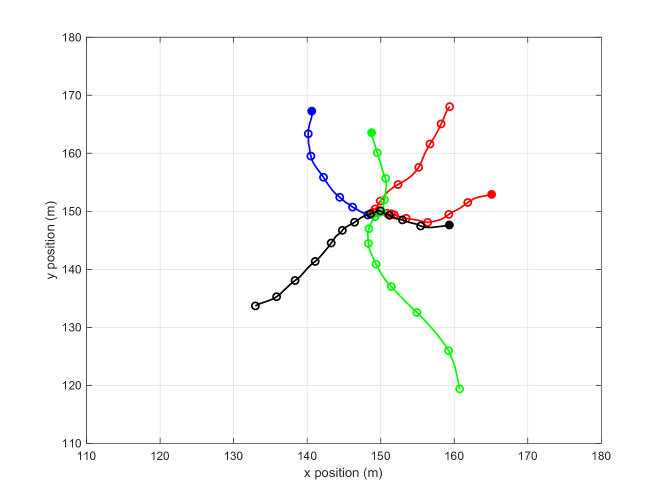
?figurename? 1: True target trajectories of the four considered targets. The blue one and the red one are born at time step 1, whereas the green one and the black one are born at time step 21. The only target that dies during the simulation is the blue target, which dies at time step 40, when all targets are in close proximity. Targets positions every 10 time steps are marked with a circle, and their initial positions with a filled circle.

We consider 81 time steps and the true target trajectories in Figure 1. For each trajectory, we initiate the midpoint (state at time step 41) from a Gaussian with mean $[150,0,150,0]^{T}$ and covariance matrix $0.01I_{4}$. The rest of the trajectory is generated by running forward and backward dynamics. This scenario is challenging due to the high number of targets in close proximity, and the fact that one target dies when targets are in close proximity.

For the PMBM filter, the Poisson birth intensity has the form $\lambda_{k}^{b}(x)=\sum_{l=1}^{n_{p}}\lambda_{k}^{b,l}\mathcal{N}(x;\bar{x}_{k}^{b,l},P_{k}^{b,l})$. For the MBM filter and the $\text{MBM}_{01}$ filter, the $l$th Bernoulli component in the MB birth density has existence probability $r_{k}^{b,l}$ and single target state density $\mathcal{N}(x;\bar{x}_{k}^{b,l},P_{k}^{b,l})$, where $1\leq l\leq n_{b}$. To evaluate the estimation performance of the compared filters under different birth parameter settings, three scenarios were simulated. In the first scenario, we consider a case where targets can be born at several known locations with low uncertainty, as in [9]. We set $n_{p}=n_{b}=4$, $\lambda_{k}^{b,l}=r_{k}^{b,l}=0.01$, and $P_{k}^{b,l}=\text{diag}([3,1,3,1])^{2}$. The mean of the Gaussian components are $\bar{x}_{k}^{b,1}=[140,0,170,0]^{T}$, $\bar{x}_{k}^{b,2}=[165,0,155,0]^{T}$, $\bar{x}_{k}^{b,3}=[150,0,160,0]^{T}$ and $\bar{x}_{k}^{b,4}=[160,0,150,0]$, respectively. In the second scenario, we consider a case where targets can be born in a broad area that covers the region of interest, as in [10]. We set $n_{p}=1$, $\lambda_{k}^{b,1}=0.04$, $n_{b}=2$, $r_{k}^{b,l}=0.02$, $\bar{x}_{k}^{b,l}=[100,0,100,0]^{T}$ and $P_{k}^{b,l}=\text{diag}([150,1,150,1])^{2}$. In the third scenario, we consider a case where targets do not generate measurements until time step 10, which means that $p_{D}=0$ for the first 10 time steps and then $p_{D}=0.9$. The value of $p_{D}$ at each time step is known by the filters. The birth parameter settings are the same as in the second scenario. It should be noted that in all scenarios the multi-Bernoulli and Poisson birth model have the same intensity (probability hypothesis density) [8, Eq. (4.129)]. This implies that birth models are as close as possible from a Kullback-Leibler divergence perspective.

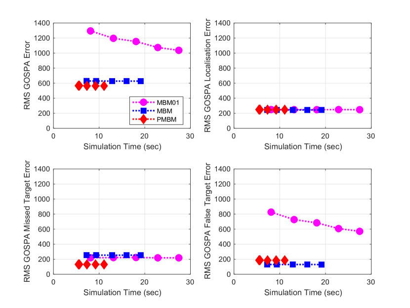
(a) Scenario 1

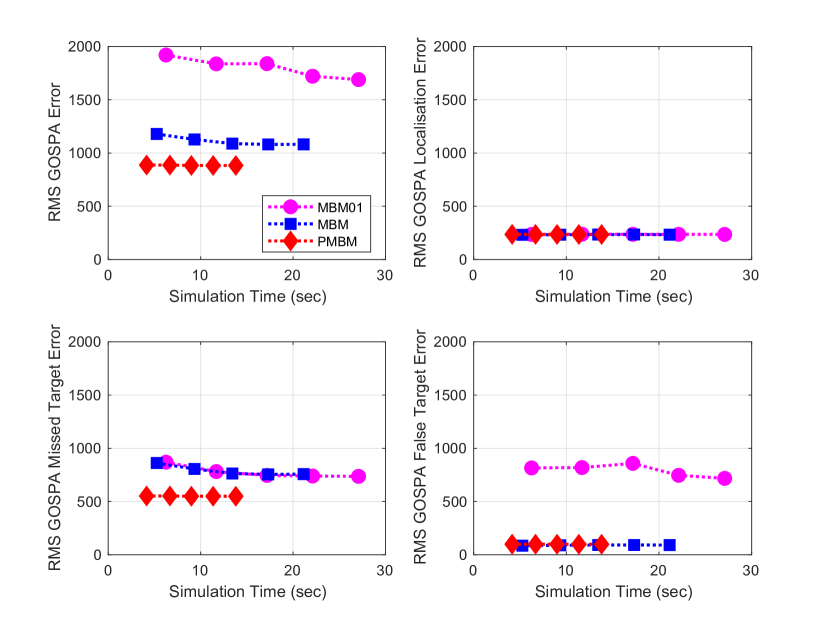
(b) Scenario 2

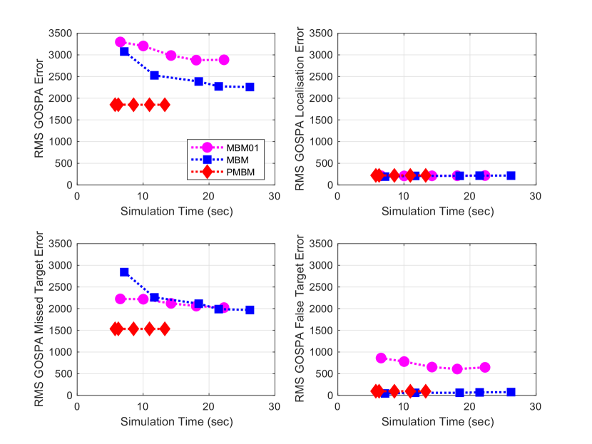
(c) Scenario 3

?figurename? 2: Performance comparison among the PMBM filter, the MBM filter and the $\text{MBM}_{01}$ ($\delta$-GLMB) filter: simulation time versus mean square GOSPA error and its decomposition. For the same filter in each sub figure, the scatter points from left to right marked with the same color correspond to $N_{h}$ equal to $100,200,300,400$ and 500.

We perform 100 Monte Carlo runs and obtain the average root mean square GOSPA error ($p=2$, $c=10$, $\alpha=2$) as well as the average running time, summed over 81 time steps for each algorithm, as shown in Figure 2. For the PMBM filter and the MBM filter, target states are extracted from Bernoulli components, contained in the MB with the highest weight, whose existence probability is above 0.4. This estimator allows two consecutive misdetections for $p_{D}=0.9$ and $p_{S}=0.99$ to report an estimate. As for the $\text{MBM}_{01}$ filter, target states are extracted from the Bernoulli components in the MB with maximum a posteriori cardinality and highest weight.

From the simulation results, we can see that the PMBM filter has the best filtering performance in terms of GOSPA error and computational time. The $\text{MBM}_{01}$ filter has significantly larger false detection error than the PMBM filter and the MBM filter. We found that this is because the filter $\text{MBM}_{01}$ usually fails to report the death of the blue target around midpoint, where targets are all in close proximity and data association becomes highly ambiguous. This observation confirms the fact that MBM parameterisation can represent the true posterior better than the $\text{MBM}_{01}$ parameterisation.

The MBM presents larger missed detection error than the PMBM filter in Scenario 1, where we have an informative birth process. This difference becomes larger when we have a broad birth prior density. This is a drawback of having an MB birth density with identical Bernoulli components, which might result in additional data association uncertainty when associating measurements to Bernoulli birth components.

The advantage of having a Poisson point process birth over a multi-Bernoulli birth can be clearly seen from the simulation result of the third scenario, in which the PMBM filter has considerable smaller GOSPA error than filters using multi-Bernoulli birth. When prior birth information is vague, it is especially advantageous to use a measurement driven approach in which new Bernoulli components are created from measurements, as in the PMBM filter.

VI Conclusions

We have proposed a Gaussian implementation of the MBM filter using Murty’s algorithm to prune the global hypotheses. The MBM filter is a special case of the PMBM filter [10, 11] that arises when the birth model is multi-Bernoulli or a mixture of multi-Bernoullis. The MBM filter can be labelled if desired, and labelling does not change the filtering recursion. Our simulation results indicate that, among the two filters that use multi-Bernoulli birth model, MBM and $\text{MBM}_{01}$, the MBM filter is superior. This is due to the fact that the way of handling global hypotheses is more efficient. However, PMBM outperforms both MBM and $\text{MBM}_{01}$ in the considered scenarios. The Gaussian implementation has been provided for Gaussian/linear models, but it can also be extended to nonlinear models using non-linear Kalman filters [27].

The PMBM, MBM and $\text{MBM}_{01}$ filters can be extended to sets of trajectories to provide full information on the trajectories followed by the targets from first principles. The $\text{MBM}_{01}$ filter (including its labelled version) and PMBM filter for sets of trajectories were introduced in [28, 19], and the corresponding MBM filter for sets of trajectories is also a special cases of the PMBM, by considering a multi-Bernoulli birth process. Full details of this filter will be provided in future work.

- [1] S. Blackman and R. Popoli, Design and Analysis of Modern Tracking Systems. Artech House, 1999.
- [2] K. Granström, L. Svensson, S. Reuter, Y. Xia, and M. Fatemi, “Likelihood-based data association for extended object tracking using sampling methods,” IEEE Transactions on Intelligent Vehicles, vol. 3, no. 1, pp. 30–45, March 2018.
- [3] D. Reid, “An algorithm for tracking multiple targets,” IEEE Transactions on Automatic Control, vol. 24, no. 6, pp. 843–854, Dec. 1979.
- [4] T. Kurien, “Issues in the design of practical multitarget tracking algorithms,” in Multitarget-Multisensor Tracking: Advanced Applications, Y. Bar-Shalom, Ed. Artech House, 1990.
- [5] S. Coraluppi and C. A. Carthel, “If a tree falls in the woods, it does make a sound: multiple-hypothesis tracking with undetected target births,” IEEE Transactions on Aerospace and Electronic Systems, vol. 50, no. 3, pp. 2379–2388, July 2014.
- [6] E. Brekke and M. Chitre, “Relationship between finite set statistics and the multiple hypothesis tracker,” IEEE Transactions on Aerospace and Electronic Systems, vol. 54, no. 4, pp. 1902–1917, Aug. 2018.
- [7] T. Fortmann, Y. Bar-Shalom, and M. Scheffe, “Sonar tracking of multiple targets using joint probabilistic data association,” IEEE Journal of Oceanic Engineering, vol. 8, no. 3, pp. 173 –184, Jul. 1983.
- [8] R. P. S. Mahler, Advances in Statistical Multisource-Multitarget Information Fusion. Artech House, 2014.
- [9] B. T. Vo and B. N. Vo, “Labeled random finite sets and multi-object conjugate priors,” IEEE Transactions on Signal Processing, vol. 61, no. 13, pp. 3460–3475, July 2013.
- [10] J. L. Williams, “Marginal multi-Bernoulli filters: RFS derivation of MHT, JIPDA and association-based MeMBer,” IEEE Transactions on Aerospace and Electronic Systems, vol. 51, no. 3, pp. 1664–1687, July 2015.
- [11] A. F. García-Fernández, J. L. Williams, K. Granström, and L. Svensson, “Poisson multi-Bernoulli mixture filter: direct derivation and implementation,” IEEE Transactions on Aerospace and Electronic Systems, vol. 54, no. 4, pp. 1883–1901, Aug. 2018.
- [12] K. G. Murty, “An algorithm for ranking all the assignments in order of increasing cost.” Operations Research, vol. 16, no. 3, pp. 682–687, 1968.
- [13] I. J. Cox and M. L. Miller, “On finding ranked assignments with application to multitarget tracking and motion correspondence,” IEEE Transactions on Aerospace and Electronic Systems, vol. 31, no. 1, pp. 486–489, Jan 1995.
- [14] I. J. Cox and S. L. Hingorani, “An efficient implementation of Reid’s multiple hypothesis tracking algorithm and its evaluation for the purpose of visual tracking,” IEEE Transactions on Pattern Analysis and Machine Intelligence, vol. 18, no. 2, pp. 138–150, Feb 1996.
- [15] A. F. García-Fernández and J. Grajal, “Multitarget tracking using the joint multitrack probability density,” in 12th International Conference on Information Fusion, July 2009, pp. 595–602.
- [16] A. F. García-Fernández, J. Grajal, and M. R. Morelande, “Two-layer particle filter for multiple target detection and tracking,” IEEE Transactions on Aerospace and Electronic Systems, vol. 49, no. 3, pp. 1569–1588, July 2013.
- [17] B.-N. Vo, B.-T. Vo, and D. Phung, “Labeled random finite sets and the Bayes multi-target tracking filter,” IEEE Transactions on Signal Processing, vol. 62, no. 24, pp. 6554–6567, Dec. 2014.
- [18] E. H. Aoki, P. K. Mandal, L. Svensson, Y. Boers, and A. Bagchi, “Labeling uncertainty in multitarget tracking,” IEEE Trans. on Aerospace and Electronic Systems, vol. 52, no. 3, pp. 1006–1020, June 2016.
- [19] A. F. García-Fernández, L. Svensson, and M. R. Morelande, “Multiple target tracking based on sets of trajectories,” accepted for publication in IEEE Transactions on Aerospace and Electronic Systems, 2015. [Online]. Available: https://arxiv.org/abs/1605.08163
- [20] L. Cament, M. Adams, and J. Correa, “A multi-sensor, Gibbs sampled, implementation of the multi-Bernoulli Poisson filter,” in 21st International Conference on Information Fusion, 2018, pp. 2580–2587.
- [21] J. L. Williams, “Hybrid Poisson and multi-Bernoulli filters,” in 15th International Conference on Information Fusion, 2012, pp. 1103 –1110.
- [22] Y. Xia, K. Granström, L. Svensson, and A. F. García-Fernández, “Performance evaluation of multi-Bernoulli conjugate priors for multi-target filtering,” in 20th International Conference on Information Fusion, July 2017, pp. 1–8.
- [23] H. W. Kuhn, “The Hungarian method for the assignment problem,” vol. 2, pp. 83–97, 1955.
- [24] A. S. Rahmathullah, A. F. García-Fernández, and L. Svensson, “Generalized optimal sub-pattern assignment metric,” in 20th International Conference on Information Fusion, 2017.
- [25] J. Correa, M. Adams, and C. Perez, “A Dirac delta mixture-based random finite set filter,” in International Conference on Control, Automation and Information Sciences, Oct. 2015, pp. 231–238.
- [26] B. N. Vo, B. T. Vo, and H. G. Hoang, “An efficient implementation of the generalized labeled multi-Bernoulli filter,” IEEE Transactions on Signal Processing, vol. 65, no. 8, pp. 1975–1987, April 2017.
- [27] S. Särkkä, Bayesian Filtering and Smoothing. Cambridge University Press, 2013.
- [28] K. Granström, L. Svensson, Y. Xia, J. L. Williams, and A. F. García-Fernández, “Poisson multi-Bernoulli mixture trackers: continuity through random finite sets of trajectories,” in 21st International Conference on Information Fusion, 2018.