Unfolding measurement distributions via quantum annealing

Abstract

High-energy physics is replete with hard computational problems and it is one of the areas where quantum computing could be used to speed up calculations. We present an implementation of likelihood-based regularized unfolding on a quantum computer. The inverse problem is recast in terms of quadratic unconstrained binary optimization (QUBO), which has the same form of the Ising hamiltonian and hence it is solvable on a programmable quantum annealer. We tested the method using a model that captures the essence of the problem, and compared the results with a baseline method commonly used in precision measurements at the Large Hadron Collider (LHC) at CERN. The unfolded distribution is in very good agreement with the original one. We also show how the method can be extended to include the effect of nuisance parameters representing sources of systematic uncertainties affecting the measurement.

1 Introduction

Problems in experimental high-energy physics have always challenged information and communication technologies. The Large Hadron Collider at CERN is a great example of this, and with its upgrade program it is crucial that the computational resources continue scaling dimeglio2017cern . Quantum computing is one the technologies that holds the promise of speeding up computationally expensive tasks. Progress has been rapid in the development of quantum computing hardware, but implementations remain imperfect. Noise and limited scalability are the primary issues, leading to the term noisy, intermediate-scale quantum (NISQ) era preskill2018quantum . Given the potential of quantum computing, there has been some exploratory work on using quantum devices in high-energy physics, for instance, in finding the Higgs boson in a simplified search domain mott2017solving , reconstruction of the trajectory of charged particles Bapst:2019llh and calculation of quantum properties of final state radiation Bauer:2019qxa . This proof-of-concept was shown on a programmable quantum annealer Johnson2011Quantum ; tanaka2017quantum , which is the largest scale quantum computer currently available. We use the same architecture to apply quantum computing in a practical problem and solve a frequently appearing task in experiments: unfolding.

Unfolding is the procedure of correcting for distortions due to limited resolution of the measuring device cowan1998statistical as found in particle physics aaboud2018measurements ; sirunyan2019measurement , astronomy hogbom1974aperture and other fields. This mathematical treatments is also known as the inverse problem or deconvolution. Unfolding is not necessary if the only goal is to compare the theory with the experimental results. In this case, a simulation of the experimental apparatus is used to account e.g. for the interaction of radiation with matter, nuclear interactions, lens distortions, etc. In practical terms, this is usually carried out using computer codes such as Geant4 agostinelli2003geant , FLUKA battistoni2011fluka , and Delphes favereau2014delphes3 . On the other hand, unfolding is essential if the aim is to compare measurements coming from different experiments. In general, each experimental apparatus has a unique signature in terms of detection efficiency, geometric acceptance and resolution. The overall effect is that the numerical value of some quantity generated in a given physical process is changed by the process of measurement. Unfolding is the mathematical procedure to “correct” for these effects and recover the original value. Solving unfolding is a computationally challenging task: in what follows, we demonstrate how to map the problem to a quantum computer to accelerate the computations with upcoming quantum hardware. Fig. 1 outlines the proposed scheme.

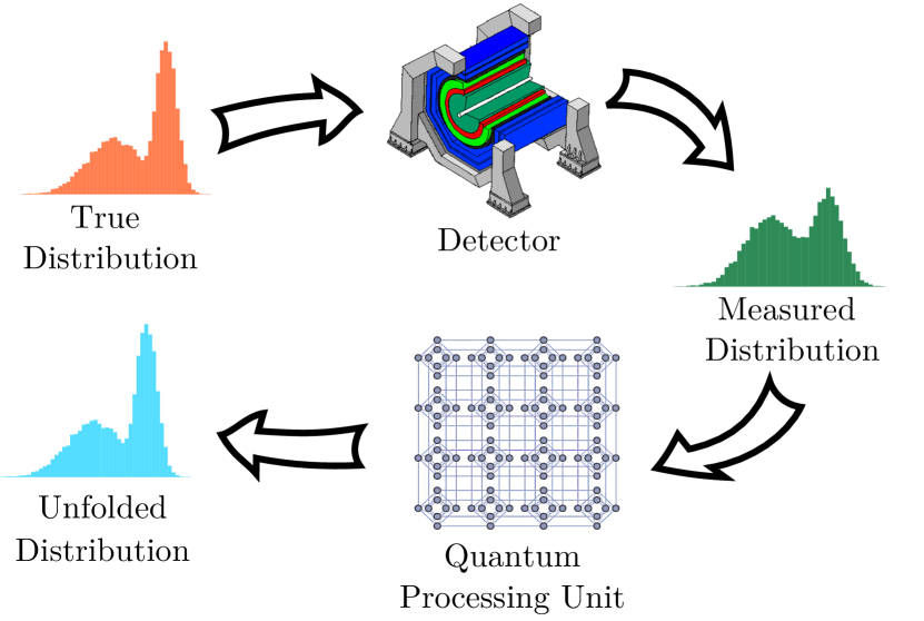
Figure 1: The unfolding procedure corrects measured distributions, removing distortions caused by the detector. Here, we implement unfolding on a quantum computer detectorImage .

Usually, the physical observable $\theta$ being measured is distributed with a probability density function $f(\theta)$ whose functional form is not known a priori. It is customary to make use of binned distributions in the form of normalized histograms. Then, probability $p_{j}$ of finding $\theta$ in the bin $j$ is simply given by the integral of $f(\theta)$ in that bin, i.e. :

$$p_{j}=\int f(\theta)d\theta.$$ (1)

The sum of all $p_{j}$ is equal to one. This probability distribution is turned into an actual physical prediction by multiplying the value of each bin by a dimensionful quantity such as a cross-section. Typically, this probability density function is estimated by simulating the physics process multiple times, using Monte Carlo methods, as it is done for example in so-called event generators such as Pythia sjostrand2008pythia or Herwig bellm2016herwig . The result of this operation is a histogram representing the “true” distribution $\theta$. After applying the effect of the experimental apparatus, one obtains another histogram corresponding to the “reconstructed” distribution $\mu$, i.e. a prediction that can be compared to a measured distribution of real data $d$.

In its simplest form, the method to unfold the measurement to the truth level is to estimate efficiency factors $\epsilon_{j}$ for each bin from the simulation:

$$\epsilon_{j}=\mu_{j}/\theta_{j}.$$ (2)

The unfolded distribution $\hat{\theta}$ is thus obtained by applying these efficiency factors to the observed data $d$ such that:

$$\hat{\theta}_{j}=\epsilon^{-1}_{j}d_{j}.$$ (3)

This method, called bin-to-bin correction, has strong limitations: the histograms representing distributions before and after interacting with the experimental apparatus (in the following referred to as truth- and reco-level respectively) must have the same binning, correlations between adjacent bins are neglected, and there is no way to account for migration of events generated in a truth bin $j$ but ending up in a reco bin $i$.

These difficulties can be overcome if we promote the efficiency correction factors $\epsilon_{j}$ to a matrix $R_{ij}$ (usually called response matrix), estimated from the simulation, such that:

$$\mu = R\theta$$ (4)

$$\hat{\theta} = R^{-1}d.$$ (5)

In principle, the number of bins at reco and truth level do not have to match, allowing also for over- and under-constrained unfolding. Typically, $R$ is presented as a matrix of (reco, truth) with rows that are normalized to unity, so that each entry is the probability that events produced in a given truth bin $j$ will be observed in the reco bin $i$. The inverse of this matrix multiplication, as applied in Eq. 5, is commonly known as unregularized matrix inversion unfolding.

Despite its relative simplicity, this method still suffers from numerical instabilities due to the inversion of the response matrix. This can be exacerbated by limitations in the simulations that may require very large computational resources to estimate off-diagonal elements with a high degree of precision. These elements encode very unlikely situations where the limited resolution causes migrations, or a dramatic drop of efficiency or acceptance due to incomplete hermiticity, lack of instrumentation and other effects. One possible approach is to constrain the truth-level distribution $\hat{\theta}$ by maximizing a likelihood function $\mathcal{L}(\mu|d)$ that depends on the estimated reco-level spectrum $\mu=\mu(\hat{\theta})$ and observed data $d$. In the case of a counting experiment, the likelihood is usually the product of Poisson or Gaussian (in the limit of large $\mu$) distributions for each bin. Ideally, the truth-level unfolded distribution $\hat{\theta}$ is expected to show a good degree of regularity. For example, there should not be sharp transitions unless otherwise anticipated from a theoretical model. Among various possibilities, the most common way to achieve this is to impose an additional constraint in the form of a Lagrange multiplier added to the likelihood function, whose effect is to favour smooth solutions. The strength of the regularization can be controlled by an additional parameter $\beta$. A common measure of smoothness to be minimized is the second derivative of the distribution. This is an example of what is known more generally as Tikhonov regularization. A similar approach to regularization is employed in the TUnfold algorithm Schmitt_2012 .

The complete likelihood to be maximized is thus:

$$\mathcal{L}(\mu|d) = \left(\prod_{i}^{N}Poiss(\mu_{i},d_{i})\right)\times e^{-\beta\rho},$$ (6)

$$Poiss(\mu_{i},d_{i}) = \frac{(\mu_{i})^{d_{i}}}{d_{i}!}e^{-\mu_{i}},$$ (7)

$$\mu_{i} = \sum_{j}^{N}R_{ij}\hat{\theta}_{j},$$ (8)

$$\rho = \sum_{j=2}^{N-1}\left(\hat{\theta}_{j+1}+\hat{\theta}_{j-1}\right)^{2}.$$ (9)

For numerical stability reasons, it is often preferable to minimize the logarithm of the likelihood, $\log\mathcal{L}(\mu|d)$. More advanced methods dagostini1995multidimensional ; choudalakis2012fully have been developed to integrate out nuisance parameters, i.e. parameters needed to account for extra variation in the model such as sources of systematic uncertainty.

2 QUBO formulation of the unfolding problem

To translate matrix operations to the quantum computing realm, an intermediate step has to be taken: the likelihood function presented in Eq. 6 has to be adapted so that the unfolding can be expressed in terms of a binary optimization, which in turn can be implemented on a quantum annealer.

The quadratic unconstrained binary optimization (QUBO) model requires the minimization of an objective function:

$$y=q^{T}Cq,$$ (10)

where $q$ is a vector of binary elements (observing that $q_{j}^{2}=q_{j}$ if $q_{j}$ can only be either 0 or 1) and $C$ is a square matrix of constants, often presented in upper triangular form. QUBO is a special case of quadratic programming. Usually, the minimization is subject to a number of constraints, which can be encoded in a quadratic penalty term, such that:

$$y = q^{T}Cq=$$ (11)

$$= \sum_{j=1}^{N}c_{jj}q_{j}q_{j}+\sum_{1\leq j<k\leq N}c_{jk}q_{j}q_{k}.$$

The linear constraints appear on the diagonal of the $C$ matrix, while the off-diagonal elements encode the quadratic penalty terms.

To rewrite the unfolding equation, we follow the approach described in Ref. omalley2016 . First, we replace the Poisson term with a sum of squares of differences, i.e. the square of the $L_{2}$ norm between the observed data and the reconstructed spectrum, which corresponds to taking the Gaussian approximation. Then, the regularization is obtained by minimizing the second derivative up to a multiplicative factor $\lambda$, which is obtained by multiplying the truth-level spectrum $x$ by the Laplacian operator $D$. Thus, the objective function to be minimized is:

$$y=\left\|Rx-d\right\|^{2}+\lambda\left\|Dx\right\|^{2}.$$ (12)

The detailed conversion of Eq. 12 into QUBO form can be found in the appendix. Among some other algebraic manipulations, we have to deal with the fact that the weights above have been derived for a real-valued vector $x$ (of $N$ elements) rather than a binary-value vector $q$ of $nN$ elements, where $n$ is the number of bits (typically a power of 2) used to encode the elements of the real-valued vector. This can easily resolved by constructing equivalent matrices that act upon the discretized version of $x$. This can be achieved by expanding $x$ as:

$$x_{i}=\alpha_{i}+\beta_{i}\sum_{j=0}^{n-1}2^{j}q_{n\times i+j}.$$ (13)

The QUBO is formulated from Equation 13, by replacing $x_{i}$ with its binary encoding.

This way, the QUBO minimization can be expressed in terms of the binary vector $q$:

$$y=\left\|R_{2}q-d\right\|^{2}+\lambda\left\|D_{2}q\right\|^{2}.$$ (14)

3 Systematic uncertainties

Sources of systematic uncertainty shift the value of each bin by a certain amount. Typically, variations corresponding to $\pm$1 standard deviation are estimated from the simulation, and an interpolation is done during the optimization. For each bin $i$, the effect of the $k$-th systematic is represented by an additional term, so that the predicted spectrum is:

$$y^{\prime}_{i}=y_{i}+\Delta y_{i}=R_{ij}x_{j}+\sum_{k}^{N_{syst}}z_{k}s_{ik}.$$ (15)

where $y$ is the central prediction, $s_{ik}$ is the variation in bin $i$ due to systematic $k$ of strength $z_{k}$.

To take the systematic effects into account, an extended vector ($\tilde{x}$) which includes the values of the systematic strengths is defined. Equally, we define extended matrices $\tilde{R}$ and $\tilde{D}$:

$$\tilde{x} = (x_{1},\ldots,x_{N}\ \vline\ z_{1},\ldots,z_{K}),$$ (16)

$$\tilde{R} = \begin{pmatrix}R_{11}&\ldots&R_{1N}&\vline&s_{11}&\ldots&s_{1K}\\ \vdots&\ddots&\vdots&\vline&\vdots&\ddots&\vdots\\ R_{N1}&\ldots&R_{NN}&\vline&s_{N1}&\ldots&s_{NK}\end{pmatrix},$$

$$\tilde{D} = \begin{pmatrix}D_{11}&\ldots&D_{1N}&\vline&0&\ldots&0\\ \vdots&\ddots&\vdots&\vline&\vdots&\ddots&\vdots\\ D_{N1}&\ldots&D_{NN}&\vline&0&\ldots&0\end{pmatrix}.$$

By replacing $x$, $R$, and $D$ in Equation 12 with $\tilde{x}$, $\tilde{R}$, and $\tilde{D}$, the values of the systematic uncertainties can be altered and the predicted spectrum will change accordingly. Generally, such an equation does not have a unique solution as it corresponds to an under-constrained problem (there are more parameters to fit at truth-level than bins at reco-level).

An additional matrix, $S$, defined by:

$$S\tilde{x}=\gamma\begin{pmatrix}\begin{matrix}0&&\\ &\ddots&\\ &&0\end{matrix}&\vline&\begin{matrix}1&&\\ &\ddots&\\ &&1\end{matrix}\end{pmatrix}\begin{pmatrix}x_{1}\\ \vdots\\ x_{N}\\ \hline\cr z_{1}\\ \vdots\\ z_{K}\end{pmatrix}.$$ (17)

is introduced to penalize large systematics. The size of the penalty is controlled by an adjustable parameter $\gamma$. The final objective function to be minimized is then given by:

$$y=\left\|\tilde{R}\tilde{x}-d\right\|^{2}+\lambda\left\|\tilde{D}\tilde{x}\right\|^{2}+\gamma\left\|S\tilde{x}\right\|^{2}.$$ (18)

In this case, the systematic shifts $z_{k}$ are being minimized simultaneously to the spectrum, with a penalty imposed for any deviation from their nominal value of 0, with a strength controlled by the parameter $\gamma$. The form of the QUBO weights which include these additional terms is given in the appendix.

4 Quantum Annealing

Many NISQ-era quantum devices such as programmable quantum annealers Johnson2011Quantum , variational quantum eigensolvers Peruzzo2014 and variational circuits farhi2014qaoa on gate-model quantum computers, or networks of degenerate optical parametric oscillators qnncloud2017qnn are proposed for solving QUBO tasks denchev2016what ; Crosson2016 ; mandra2018deceptive . In most cases, the QUBO is mapped to a classical Ising model with a simple change of variables. This includes the D-Wave 2000Q quantum annealer with 2038 manufactured spins that our experiments relied on. On this device, the coupling and onsite fields of the Ising model are bounded the following way:

$$\hat{H}=\sum_{i,j}J_{ij}\hat{\sigma}^{z}_{i}\hat{\sigma}^{z}_{j}+\sum_{i}h_{i}\hat{\sigma}^{z}_{i}$$ (19)

$$J_{ij}\in[-1,1],h_{i}\in[-2,2],$$

where $\hat{H}$ is the cost Hamiltonian for which the annealer attempts to find the ground state.

5 Results

We tested the method described above in a realistic situation, where the quantity to be unfolded is represented by a histogram with 5 bins and migrations are not negligible (i.e.  non-zero off-diagonal elements in the response matrix). We assume that the distortions introduced by the detector are perfectly known. Hence, in order to obtain the corresponding reco-level histograms, we applied the same response matrix to the truth-level distributions of both $\mu$ and $d$, which are different in the most general case. The pseudo-data reco-level histogram is then unfolded using the following methods: D’Agostini iterative Bayesian dagostini1995multidimensional with $N_{itr}=4$; QUBO solved on the CPU by the neal simulator neal ; and QUBO executed by the real DWave QPU, with the regularization strength $\lambda$ set values between 0 and 1. The number of iterations in the benchmark unfolding method was set to 4 as a compromise between bias and statistical uncertainty. This setting is a common choice in measurements at the LHC aaboud2018measurements ; cms2017diffxs . The uncertainty is calculated from the square root of the diagonals of the covariance matrix given by the unfolding, as implemented in the RooUnfold package RooUnfold . The uncertainty associated to the unfolding quantum annealing represents one standard deviation calculated on a set of 20 executions with 5,000 reads from the QPU per run.

A first test is shown in Fig. 2, where a peaking distribution is unfolded. This is representative of the mass spectrum in presence of a resonance. All the unfolding methods are able to recover the truth-level distribution, with an agreement always in the order of about one standard deviation. There is no apparent difference between the lower-noise annealer DW_2000Q_5 solver and the older regular-noise DW_2000Q_2_1.

Fig. 3 shows the unfolding applied to a steeply falling spectrum, representative of a certain class of observables such as the transverse momentum of a particle. In this case, the unregularized QUBO is in good agreement with both the truth distribution and the D’Agostini method within one standard deviation. The impact of the regularization is evident as larger and larger values of the $\lambda$ parameter result in flatter and flatter solutions which do not agree well with the truth level. This is a confirmation of the well-known fact that the regularization is problem-dependent, and an optimal value of its strength has to be carefully estimated e.g.  from the simulation.

The good agreement with the simulated annealing and with the D’Agostini method indicates that with a large enough numerical precision, the QUBO unfolding would have a comparable performance with the traditional methods. On the other hand, the execution on the QPU is less accurate due to hardware limitations.

A further test was performed to compare the difference between a 4-bit and 8-bit encoding. The result is shown in Fig. 4. In principle, with more bits it should be possible to have a better numerical precision. However, it also results in longer chains of qbits in the minor embedding.

To test the effect of systematic uncertainties, we added one component to the pseudo-data: a shape systematic whose effect is to distort the number of entries in each bin. We set the strength of this systematic to -0.75. The unfolding is shown in Fig. 5. The discretized nature of the optimization introduces some interesting features. For this particular setup, the full solution is not degenerate, even when no penalty is applied for increasing the systematic uncertainty (i.e. $\gamma=0$). In this case, the simulated annealing correctly picks the value of the systematic and each bin of the distribution. The QPU also picks out this solution on average.

If a sufficiently large penalty parameter is applied (in this case, $\gamma$=1000), the annealing prefers a value of the systematic strength close to zero. In order to accommodate this choice, the bins gets shifted. The solution found by the simulated annealer in this case matches the brute force solution, however this solution is not found by the QPU. While more work remains to understand many subtleties, a more refined version of this methodology could be used to estimate the impacts of systematic uncertainties. This is an area for continued work.

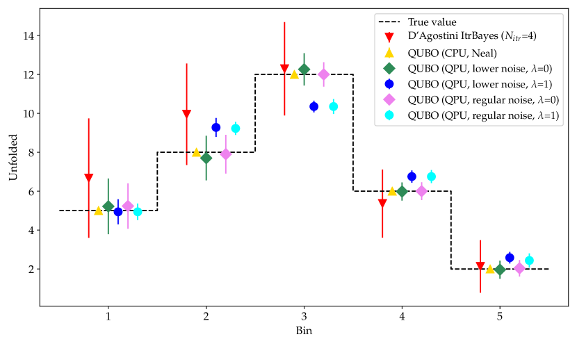
Figure 2: Truth-level distribution of pseudo-data, unfolded with different methods, of a peaked spectrum. The data corresponding to runs submitted to the QPU are averaged over 20 executions with 5000 reads each.

Figure 3: Truth-level distribution of pseudo-data, unfolded with different methods and values of the regularization strength $\lambda$, of a steeply-falling spectrum. The data corresponding to runs submitted to the QPU are averaged over 20 executions with 5000 reads each.

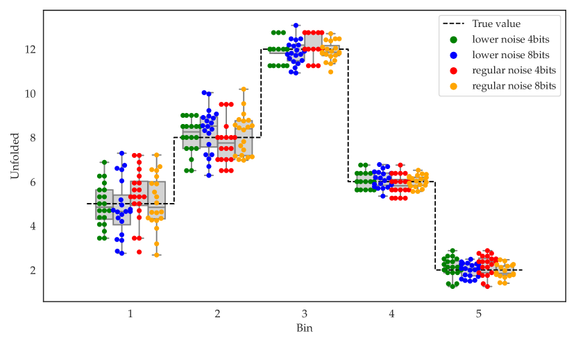
Figure 4: Truth-level distribution of pseudo-data, unfolded with either a 4- or 8-bits encoding, of a peaked spectrum. The data corresponding to runs submitted to the QPU are averaged over 20 executions with 5000 reads each. The maximum chain length in the best embedding is 7 and 15 qbits respectively. The 8-bit encoding allows a more fine-grained estimation of the unfolded histogram.

Figure 5: Truth-level distribution of pseudo-data, unfolded with different methods, of a peaked spectrum including the effect of a shape systematic. The data corresponding to runs submitted to the QPU are averaged over 20 executions with 5000 reads each.

Finally, we used the DWave-Hybrid software framework to find the solution by searching for the state of minimum energy using a Tabu heuristic algorithm glover1989tabu ; glover1990tabu and the QPU in parallel. The result we obtained is completely in agreement with both the truth-level distribution and the one obtained with the simulated annealing. While the hybrid approach goes well beyond the needs of the scenario under consideration, we argue that this is likely to be the key for a typical measurement at the LHC where the number of bins is larger than 10 and the number of sources of systematic uncertainty is on the order of 100.

6 Conclusions

NISQ-era quantum devices are meant to work in close integration with classical computing resources, creating hybrid classical-quantum algorithms. We found that using the quantum annealer together with a classical optimization metaheuristics helps with two problems: (1) problems larger than the hardware spin system can be solved; (2) results are quickly refined into the optimal solutions in a few iterations between the quantum hardware and the classical algorithm. The close agreement between the correct results and the one obtained by the hybrid classical-quantum protocol indicates the relevance of this paradigm to practical problems in experimental high-energy physics.

Upcoming quantum hardware, like the Pegasus architecture that has a denser connectivity and over five thousand qubits dattani2019pegasus , could easily tilt the balance towards the quantum part of the protocol, yielding faster time to solution compared to a purely classical solver. The scheme we introduced here may also be amenable to taking into account discretization effects, which can be significant in problems with low statistics gaponenko2019practical . The test case presented in this paper was limited to five bins in order to fit in the currently available hardware. However, the above considerations indicate that it will be possible to unfold histograms with more bins, a higher precision due to an encoding with more bits, and a larger number of systematics by the means of the integration of more powerful and less noisy QPUs with classical systems based on CPUs.

Appendix

This appendix gives the detailed derivation of mapping the unfolding problem to a quadratic unconstrained binary optimization (QUBO). After deriving the basic formulation with Tikhonov regularization, we add an additional regularization term for systematic uncertainties.

Deriving the QUBO formulation of the unfolding problem To rewrite the unfolding equation, we follow the approach described in Ref. omalley2016 . First, we replace the Poisson term with a sum of squares of differences, i.e. the square of the $L_{2}$ norm between the observed data and the reconstructed spectrum. Then, the regularization is obtained by minimizing the second derivative, which is obtained by multiplying the truth-level spectrum $x$ by the Laplacian operator, e.g. :

$$D=\begin{pmatrix}-2&1&0&0&0\\ 1&-2&1&0&0\\ 0&1&-2&1&0\\ 0&0&1&-2&1\\ 0&0&0&1&-2\end{pmatrix}.$$ (20)

Other regularization choices are possible, but the second derivative is a common choice, and used for the calculations in this paper. The relative strengths of the regularization term (as compared to the agreement between the data and the reconstructed spectrum) is controlled by a parameter, $\lambda$. Thus, the objective function to be minimized is:

$$y=\left\|Rx-d\right\|^{2}+\lambda\left\|Dx\right\|^{2}.$$ (21)

To convert Eq. 21 into QUBO form such as Eq. (12) in the main text, we rewrite the equations using index notation, i.e.:

$$Ax \to A_{ij}x_{j},$$ (22)

$$AB \to A_{ij}B_{jk},$$ (23)

$$AB^{T} \to A_{ij}B_{ik}.$$ (24)

A summation over repeated indices is implicit, unless otherwise noted. Thus, we have:

$$y = \left(R_{ij}x_{j}-d_{i}\right)\left(R_{ik}x_{k}-d_{i}\right)+\lambda\left(D_{ij}x_{j}D_{ik}x_{k}\right)$$

$$= \left(R_{ij}R_{ik}+\lambda D_{ij}D_{ik}\right)x_{j}x_{k}-2R_{ij}x_{j}d_{i}+d_{i}d_{i}$$

The term $d_{i}d_{i}$ can be ignored, since it adds a constant, which does not affect the optimization. Before determining the QUBO weights, we need to encode the floating point values $x_{i}$ into an appropriate binary format for the QUBO.

The simplest encoding, which is suitable for some situations, is a standard n-bit integer encoding:

$$x_{i}=\sum_{j=0}^{n-1}2^{j}q_{n\times i+j},$$ (26)

where $q_{a}\in\{0,1\}$. However, this is somewhat limiting for two reasons: firstly, this limits the values to positive integers; secondly, current quantum computing hardware requires the bit encodings to be small, which may put limitations on the range of values which can be encoded.

Standard floating point encodings do not lend themselves naturally to the QUBO problem because the exponent bits give rise to non-quadratic terms. Here, we chose to use a non-standard encoding. Each value $x_{i}$ is encoded with $n$ bits using an offset, $\alpha_{i}$, and a scaling parameter, $\beta_{i}$:

$$x_{i}=\alpha_{i}+\beta_{i}\sum_{j=0}^{n-1}2^{j}q_{n\times i+j}.$$ (27)

The values of the offset and scaling parameters are stored on the classical computer, so that they can be used to encode and decode the the QUBO results. In order to provide additional flexibility, each value in $\vec{x}$ may be encoded with a different number of bits. This flexibility is implemented in the code, but for clarity of exposition, the fixed-bit encoding is given here. To simplify the notation, we define $\beta_{ia}$ instead of writing the sum over $j$:

$$x_{i}=\alpha_{i}+\beta_{ia}q_{a}.$$ (28)

Defining $a_{0}\equiv i\times n$, we can reproduce Equation 27 by setting $\beta_{ia}=\beta_{i}2^{(a-a_{0})}$ for $0\leq(a-a_{0})<n$ and 0 otherwise. The QUBO is formulated from Equation Appendix, by replacing $x_{i}$ with its binary encoding. Additionally, for notational convenience, we define $W_{jk}\equiv(R_{ij}R_{ik}+\lambda D_{ij}D_{ik})$. This gives:

$$y = W_{jk}\alpha_{j}\alpha_{k}+2W_{jk}\alpha_{j}\beta_{ka}q_{a}$$ (29)

$$+W_{jk}\beta_{ja}\beta_{kb}q_{a}q_{b}$$

$$-2R_{ij}d_{i}\alpha_{j}-2R_{ij}d_{i}\beta_{ja}q_{a}+d_{i}d_{i}.$$

As before, constant terms (those not containing $q_{a}$) have no impact on the optimization; therefore, the terms $W_{jk}\alpha_{j}\alpha_{k}$, $R_{ij}d_{i}\alpha_{j}$, and $d_{i}d_{i}$ can be ignored. Expressing in terms of the binary values $q_{a}$, we also have $q_{a}q_{a}=q_{a}$. So that for $a=b$ the term $W_{jk}\beta_{ja}\beta_{kb}q_{a}q_{b}$ can be rewritten as simply $W_{jk}\beta_{ja}\beta_{ka}q_{a}$. Enforcing the requirement $a<b$ then Equation 29 can be rewritten in QUBO form as:

$$y^{\prime}=\sum_{a=1}^{N}c_{aa}q_{a}q_{a}+\sum_{a<b}c_{ab}q_{a}q_{b};$$

with:

$$c_{ab} = 2W_{jk}\beta_{ja}\beta_{kb},$$ (30)

$$c_{aa} = 2W_{jk}\alpha_{k}\beta_{ja}+$$ (31)

$$W_{jk}\beta_{ja}\beta_{ka}-2R_{ij}d_{i}\beta_{ja}.$$

The repeated index $a$ is not summed over in Equation 31.

In general, determining the parameters $\alpha_{i}$ and $\beta_{i}$ is a problem-specific task. They define the space of possible solutions, and therefore can be chosen to force certain constraints. For example, for problems where $\vec{x}\in\mathbb{N}$ choosing $\alpha_{i}$, $\beta_{i}\in\mathbb{N}$ will ensure the solution also respects this form. Nonetheless, the solution will only span a certain range. We use a heuristic to form initial guesses for suitable choices. Additional heuristics and criteria for updating the values based on results can be developed in a straightforward manner.

QUBO weights with systematic uncertainties— Only a minor modification of the above derivation is required to include the case of systematic uncertainties. The QUBO weights for the vector $\tilde{q}$, corresponding to the binary encoding of $\tilde{x}$ proceeds by replacing Equation Appendix with Equation 18 and following the derivation above. The result of the calculation is that the QUBO weights for $\tilde{q}$ are then as given in Equations 30 and 31 but with $W_{ij}=\tilde{R}_{ij}\tilde{R}_{ij}+\lambda\tilde{D}_{ij}\tilde{D}_{ij}+\gamma S_{ij}S_{ij}$.

In fact, Equation 18 can be transformed into the form of Equation Appendix by defining a matrix:

$$\tilde{D^{\prime}}=\begin{pmatrix}\tilde{D}\\ \hline\cr\sqrt{\frac{\gamma}{\lambda}}S\end{pmatrix}$$

which is of block diagonal form and treats the regularization and systematic uncertainties in a single term. Then, the form of $W_{ij}$ follows from direct substitution.

References

- (1) A. Di Meglio, M. Girone, A. Purcell, and F. Rademakers, “Cern openlab whitepaper on future it challenges in scientific research,” 2017.
- (2) J. Preskill, “Quantum computing in the NISQ era and beyond,” Quantum, vol. 2, p. 79, 2018.
- (3) A. Mott, J. Job, J.-R. Vlimant, D. Lidar, and M. Spiropulu, “Solving a Higgs optimization problem with quantum annealing for machine learning,” Nature, vol. 550, no. 7676, p. 375–379, 2017.
- (4) F. Bapst, W. Bhimji, P. Calafiura, H. Gray, W. Lavrijsen, and L. Linder, “A pattern recognition algorithm for quantum annealers,” 2019.
- (5) C. W. Bauer, B. Nachman, D. Provasoli, and W. A. De Jong, “A quantum algorithm for high energy physics simulations,” 2019.
- (6) M. W. Johnson, M. H. S. Amin, S. Gildert, T. Lanting, F. Hamze, N. Dickson, R. Harris, A. J. Berkley, J. Johansson, P. Bunyk, E. M. Chapple, C. Enderud, J. P. Hilton, K. Karimi, E. Ladizinsky, N. Ladizinsky, T. Oh, I. Perminov, C. Rich, M. C. Thom, E. Tolkacheva, C. J. S. Truncik, S. Uchaikin, J. Wang, B. Wilson, and G. Rose, “Quantum annealing with manufactured spins,” Nature, vol. 473, p. 194–198, May 2011.
- (7) S. Tanaka, R. Tamura, and B. K. Chakrabarti, Quantum spin glasses, annealing and computation. Cambridge University Press, 2017.
- (8) G. Cowan, Statistical data analysis. Oxford University Press, 1998.
- (9) The ATLAS Collaboration, “Measurements of differential cross-sections of highly boosted top quarks decaying to all-hadronic final states in pp collisions at = 13 tev using the ATLAS detector,” Physical Review D, vol. 98, no. 1, p. 012003, 2018.
- (10) The CMS Collaboration, “Measurement of inclusive and differential Higgs boson production cross sections in the diphoton decay channel in proton-proton collisions at = 13 TeV,” Journal of High Energy Physics, vol. 2019, no. 1, p. 183, 2019.
- (11) J. Högbom, “Aperture synthesis with a non-regular distribution of interferometer baselines,” Astronomy and Astrophysics Supplement Series, vol. 15, p. 417, 1974.
- (12) GEANT4 Collaboration, “Geant4—a simulation toolkit,” Nuclear Instruments and Methods in Physics Research Section A: Accelerators, Spectrometers, Detectors and Associated Equipment, vol. 506, no. 3, pp. 250–303, 2003.
- (13) G. Battistoni, A. Margiotta, S. Muraro, and M. Sioli, “FLUKA as a new high energy cosmic ray generator,” Nuclear Instruments and Methods in Physics Research Section A: Accelerators, Spectrometers, Detectors and Associated Equipment, vol. 626-627, pp. S191–S192, 2011.
- (14) J. de Favereau, , C. Delaere, P. Demin, A. Giammanco, V. Lemaître, A. Mertens, and M. Selvaggi, “DELPHES 3: a modular framework for fast simulation of a generic collider experiment,” Journal of High Energy Physics, vol. 2014, no. 2, p. 57, 2014.
- (15) “Detector image slightly modified from source.” http://www.particleadventure.org/modern_detect.html. Accessed: 2019-08-07.
- (16) T. Sjöstrand, S. Mrenna, and P. Skands, “A brief introduction to PYTHIA 8.1,” Computer Physics Communications, vol. 178, no. 11, pp. 852–867, 2008.
- (17) J. Bellm, S. Gieseke, D. Grellscheid, S. Plätzer, M. Rauch, C. Reuschle, P. Richardson, P. Schichtel, M. H. Seymour, A. Siódmok, A. Wilcock, N. Fischer, M. A. Harrendorf, G. Nail, A. Papaefstathiou, and D. Rauch, “Herwig 7.0/herwig 3.0 release note,” The European Physical Journal C, vol. 76, no. 4, p. 196, 2016.
- (18) S. Schmitt, “TUnfold, an algorithm for correcting migration effects in high energy physics,” Journal of Instrumentation, vol. 7, pp. T10003–T10003, oct 2012.
- (19) G. D’Agostini, “A multidimensional unfolding method based on Bayes’ theorem,” Nuclear Instruments and Methods in Physics Research Section A: Accelerators, Spectrometers, Detectors and Associated Equipment, vol. 362, no. 2-3, pp. 487–498, 1995.
- (20) G. Choudalakis, “Fully Bayesian unfolding,” 2012.
- (21) D. O’Malley and V. V. Vesselinov, “ToQ.jl: A high-level programming language for D-Wave machines based on Julia,” in 2016 IEEE High Performance Extreme Computing Conference (HPEC), 2016.
- (22) A. Peruzzo, J. McClean, P. Shadbolt, M.-H. Yung, X.-Q. Zhou, P. J. Love, A. Aspuru-Guzik, and J. L. O’Brien, “A variational eigenvalue solver on a photonic quantum processor,” Nat. Commun., vol. 5, p. 4213, dec 2014.
- (23) E. Farhi, J. Goldstone, and S. Gutmann, “A Quantum Approximate Optimization Algorithm,” tech. rep., MIT, nov 2014.
- (24) QNNCloud, “Quantum neural network: Optical neural networks operating at the quantum limit,” 2017.
- (25) V. S. Denchev, S. Boixo, S. V. Isakov, N. Ding, R. Babbush, V. Smelyanskiy, J. Martinis, and H. Neven, “What is the computational value of finite range tunneling?,” Physical Review X, vol. 6, p. 031015, Aug. 2016.
- (26) E. Crosson and A. W. Harrow, “Simulated Quantum Annealing Can Be Exponentially Faster Than Classical Simulated Annealing,” in 2016 IEEE 57th Annu. Symp. Found. Comput. Sci., vol. 2016-Decem, pp. 714–723, IEEE, oct 2016.
- (27) S. Mandrá and H. G. Katzgraber, “A deceptive step towards quantum speedup detection,” Quantum Science and Technology, vol. 3, no. 4, p. 04LT01, 2018.
- (28) “Simulated annealing sampler.”
- (29) The CMS Collaboration, “Measurement of differential cross sections for the production of top quark pairs and of additional jets in lepton+jets events from pp collisions at 13 TeV,” Phys. Rev. D, vol. 97, p. 112003. 91 p, Mar 2018. * Temporary entry *.
- (30) CERN, PHYSTAT 2011 Workshop on Statistical Issues Related to Discovery Claims in Search Experiments and Unfolding, (Geneva), CERN, 2011.
- (31) F. Glover, “Tabu search—Part I,” ORSA Journal on Computing, vol. 1, no. 3, pp. 190–206, 1989.
- (32) F. Glover, “Tabu search—Part II,” ORSA Journal on Computing, vol. 2, no. 1, pp. 4–32, 1990.
- (33) N. Dattani, S. Szalay, and N. Chancellor, “Pegasus: The second connectivity graph for large-scale quantum annealing hardware,” 2019.
- (34) A. Gaponenko, “A practical way to regularize unfolding of sharply varying spectra with low data statistics,” 2019.