LCTP-19-18

Aspects of AdS₂ classification in M-theory:

Solutions with mesonic and baryonic charges

Junho Hong^a, Niall T. Macpherson^b and Leopoldo A. Pando Zayas^c

^a,c Leinweber Center for Theoretical Physics, Department of Physics
University of Michigan, Ann Arbor, MI 48109, USA

^b SISSA International School for Advanced Studies
Via Bonomea 265, 34136 Trieste
and
INFN, sezione di Trieste

^c The Abdus Salam International Centre for Theoretical Physics
Strada Costiera 11, 34014 Trieste, Italy

We construct necessary and sufficient geometric conditions for a class of AdS₂ solutions of M-theory with, at least, minimal supersymmetry to exist. We generalize previous results in the literature for ${\cal N}=(2,0)$ supersymmetry in AdS₂ to ${\cal N}=(1,0)$. When the solution can be locally described as AdS${}_{2}\times\Sigma_{g}\times\,$SE₇ with $\Sigma_{g}$ a Riemann surface of genus $g$ and SE₇ a seven-dimensional Sasaki-Einstein manifold, we clarify and unify various solutions present in the literature. In the case of SE${}_{7}=Q^{1,1,1}$ we find a new solution with baryonic and mesonic charges turned on simultaneously.

junhoh@umich.edu, nmacpher@sissa.it, lpandoz@umich.edu

1 Introduction

Our understanding of asymptotically AdS₄ black holes has recently undergone a revolutionary transformation. Via the AdS/CFT correspondence the macroscopic entropy of a large class of asymptotically AdS₄ black holes has been given a microscopic explanation in terms of states in the dual 3d ${\cal N}=2$ supersymmetric field theories. Namely, it has been shown that the topologically twisted index in field theory accounts for the macroscopic entropy of magnetically charged asymptotically AdS₄ black holes [1, 2]. The original observation has been generalized to include various situations: black holes with hyperbolic horizons [3], black holes in massive type IIA supergravity [4, 5], black holes in universal sectors of gauged supergravities related to M2 branes [6] and to M5 branes [7] (for reviews with complete lists of references, see [8, 9]).

This remarkable progress points to an interesting gap – there seem to be a number of black hole solutions missing. Namely, there are various field theory results for which the dual black holes are not yet known; this is a welcome challenge for the supergravity community. For example, the topologically twisted index can be computed for a fairly generic class of 3d ${\cal N}=2$ supersymmetric field theories, many of which have known gravity duals [12, 13]. In particular, there are results for field theory duals to AdS${}_{4}\times\,$SE₇ when SE${}_{7}=\{S^{7},Q^{1,1,1},M^{1,1,1},V^{5,2},N^{0,1,0}\}$. The first entry in this list is well understood on the black hole side [1, 2], thanks to known solutions in gauged supergravity [14] and their eleven-dimensional uplift [15], which includes the vector multiplets associated to the isometry of $S^{7}$ and therefore the mesonic charges in the field theory side. For the other entries, the eleven-dimensional uplifts with the corresponding vector and hyper mutiplets are also known [16]. In these cases, however, the vector multiplets are associated to the non-trivial two cycles of the internal manifolds and not to isometries of the space. This implies that the eleven-dimensional uplift with the internal manifolds $Q^{1,1,1},M^{1,1,1},V^{5,2},N^{0,1,0}$ allows only for the AdS₄ black holes whose $U(1)$ charges are baryonic in the field theory side, which has been studied in [17, 18]: the AdS₄ black hole solutions with mesonic twists are still missing in this case. Considering that the dual topologically twisted indices with mesonic charges have been already computed in many examples [12, 13], finding such black holes is an interesting and important problem which might generalize the match found in [1, 2] to general SE₇ internal manifolds.

In this manuscript we do not directly tackle the construction of such missing black holes, rather, we focus on a more modest problem. We focus on understanding the near horizon geometry of those extremal black holes. Such solution must contain an AdS₂ region and, in all the known cases, it turns out that the near horizon region is by itself a solution of the supergravity equations of motion. Thus, the classification of solutions with an AdS₂ factor although motivated by understanding extremal black holes in AdS₄ is a well-defined problem in supergravity. In this manuscript we take some steps into the full systematic classification. We will, however, be guided by a particularly interesting class of solutions – AdS${}_{4}\times\,$SE₇ – whose relation to the black hole is presaged by various field theory computations.

There have been various explicit efforts towards constructing solutions with AdS₂ factors, for example, [19, 20, 21, 22]. There are other approaches more focused on constructing new solutions and downplaying a classificatory goal such as in [6]. One of our goals in this manuscript is to take one systematic step towards a complete classification within a well-defined class. Another important goal of this paper is to present explicit solutions capable of elucidating some of the current puzzles marring the gravitational understanding of some of the topologically twisted indices on the dual field theory.

The rest of the manuscript is organized as follows. In section 2 we discuss general conditions for the existence of supersymmetric AdS₂ solution in M-theory supporting an SU(4)-structure. We pay particular attention to differences between ${\cal N}=(1,0)$ and ${\cal N}=(2,0)$. Section 3 starts by briefly describing a number of puzzling situations regarding the entropy of asymptotically AdS₄ solutions from the AdS/CFT point of view. We then proceed to cast a number of known solutions within our classificatory scheme and also present the details and motivation for the construction of new solutions with baryonic and mesonic charges turned on. In appendix A we demonstrate the absence of AdS₂ solutions in M-theory with Spin(7)-structure, while in appendix B show that no AdS₃ solutions follow from SU(4) structure. We also present some explicit details of the Killing spinor equations in appendix C to aid readers who prefer a more classic approach to solution building.

2 AdS₂ solutions with SU(4)-structure

In this section we will derive sufficient geometric conditions for a certain class of minimally supersymmetic AdS₂ solutions in M-theory to exist. The class in question consists of internal spaces that support an SU(4)-structure. From these conditions we also derive necessary conditions for $\mathcal{N}=(2,0)$ with SU(4)-structure, which turn out to coincide with those presented in [21].

2.1 Supersymmetric AdS₂

The most general form of a solution to 11 dimensional supergravity that respects the isometries of AdS₂ can take a metric and flux that can be decomposed as

$$ds^{2}=e^{2A}ds^{2}(\text{AdS}_{2})+ds^{2}(\text{M}_{9}),~{}~{}~{}~{}~{}F=e^{2A}\text{vol}(\text{AdS}_{2})\wedge G_{2}+G_{4},$$ (2.1)

where $e^{2A}$ depends on directions on M₉ only, and likewise the 2 and 4 forms $G_{2}$, $G_{4}$. We will allow for non trivial $G_{4}$, so we have both electric and magnetic flux components turned on in general, which should be contrasted with [19] that only considered the former. In terms of (2.1) the Bianchi identity of the flux, away from possible localised sources, becomes

$$d(e^{2A}G_{2})=0,~{}~{}~{}~{}dG_{4}=0,$$ (2.2)

while its equation of motion is implied by

$$d(e^{2A}\star_{9}G_{4})+e^{2A}G_{2}\wedge G_{4}=0,$$ (2.3a)

$$d\star_{9}G_{2}-\frac{1}{2}G_{4}\wedge G_{4}=0.$$ (2.3b)

Of course, for a solution to exist one also needs to solve Einstein’s equation, however, as we shall establish later, for the class of supersymmetric solution we are interested in it turns out that these are implied by (2.2) and (2.3b).

When supersymmetric, an M-theory solution supports an associated 11 dimensional Killing spinor $\epsilon$ that obeys

$$\nabla_{N}\epsilon+\frac{1}{4!}\bigg{(}3F\Gamma_{N}-\Gamma_{N}F\bigg{)}\epsilon=0,$$ (2.4)

where in this expression $F$ should be understood as acting under the Clifford map $F\to\frac{1}{4!}F_{MNPQ}\Gamma^{NMPQ}$. For AdS₂ solutions we may decompose $\epsilon$ in general as

$$\epsilon=\zeta_{+}\otimes\chi_{1}+\zeta_{-}\otimes\chi_{2},$$ (2.5)

where $\chi_{1,2}$ are two Majorana spinors on M₉ and $\zeta_{\pm}$ are Majorana Killing spinors on unit AdS₂ of $\pm$ chirality, and so obey

$$\nabla_{a}\zeta_{\pm}=\frac{1}{2}\gamma_{a}\zeta_{\mp}.$$ (2.6)

Upon plugging (2.5) into (2.4) it is then a rather simple matter to show that

$$|\chi|^{2}=e^{A},~{}~{}~{}~{}\chi=\frac{1}{\sqrt{2}}(\chi_{1}+i\chi_{2}),$$ (2.7)

where in the first equality we fix an arbitrary constant without loss of generality. One could proceed in kind, using the Killing spinor equations to construct spinor bi-linears and the set of necessary and sufficient geometric conditions they must obey for supersymmetry to be satisfied. However, a more efficient approach is build on an existing geometric classification, namely that of the geometry following from a single arbitrary Killing spinor in 11 dimensions [23, 24]. This derivation is similar to those in [25, 26], which look at related problems from the same geometric starting point.

2.2 Review of the Geometry of 11 dimensional Killing spinors

In [23, 24] the geometry that follows from a single Majorana Killing spinor $\epsilon$ in M-theory is classified. The fundamental objects of this construction are the 1,2 and 5-forms with components defined in terms on $\epsilon$ as

$$K_{M} =\overline{\epsilon}\Gamma_{M}\epsilon,$$ (2.8)

$$\Xi_{MN} =\overline{\epsilon}\Gamma_{MN}\epsilon,$$ (2.9)

$$\Sigma_{MNOPQ} =\overline{\epsilon}\Gamma_{MNOPQ}\epsilon,$$ (2.10)

respectively, which obey the following algebraic relations

$$\iota_{K}\Xi=0,~{}~{}~{}~{}\iota_{K}\Sigma=\frac{1}{2}\Xi\wedge\Xi,$$ (2.11)

among others. Using only the Killing spinor equation (2.4), the authors of [23] were able to establish the following necessary and sufficient geometric conditions for supersymmetry

$$d\Xi =\iota_{K}F,$$ (2.12)

$$d\Sigma =\iota_{K}\star F-\Xi\wedge F,$$ (2.13)

$$dK =\frac{2}{3}\iota_{\Xi}F+\frac{1}{3}\iota_{\Sigma}\star F,$$ (2.14)

and that $K$ is a nowhere vanishing Killing vector of both the metric and 4-form flux that can be either time-like or null. The time-like case was considered in [23] where (2.12)-(2.14) were shown to be sufficient conditions for supersymmetry with the specific analysis performed with respect to an SU(5)-structure (see for instance [27] for a review of SU(N) structures) supported by the internal space orthogonal to $K$. In [24] the null case was studied, where (2.12)-(2.14) were once more found to be sufficient for supersymmetry giving rise to a $(\text{spin}(7)\ltimes\mathbb{R}^{8})\times\mathbb{R}$-structure. In the time-like case supersymmetry together with the the Bianchi identity and equation of motion of the flux implies Einstein’s equations, while in the null case one needs to still solve one component of Einstein’s equations.

In what follows we will be interested in AdS₂ solutions that support an SU(4)-structure on their internal space (we also rule out the possibility of Spin(7)-structure in appendix A), as we shall see, for these $K$ is necessarily time-like. In principle one could work with the SU(5)-structure conditions presented in [23], however we find it easier to work directly with (2.12)-(2.14). Before moving on, let us stress that this class of solutions is by no means exhaustive - indeed all AdS₃ solutions admit a parametrisation in terms of an AdS₂ factor, and we prove in appendix B that no such solutions lie in this class.

2.3 $\mathcal{N}=(1,0)$ AdS₂ solutions with symplectic SU(4)-structure

Our task in this section is to derive $K,\Xi,\Sigma$ under the assumption that a solution decomposes as a warped product of AdS${}_{2}\times\text{M}_{9}$, with M₉ supporting an SU(4)-structure. Then we derive sufficient conditions for a supersymmetric solution in terms of geometric conditions on the SU(4)-strucutre. To this end we need to know the form the bi-linears take on AdS₂ and for an SU(4)-structure in 9 dimensions.

2.3.1 Bi-linears in 11d in terms of those on AdS₂ and M₉

The bi-linears for AdS₂ can be derived in general from the Killing spinor equation (2.6), indeed this was already done in [28] so we will be brief and refer the reader to that reference for further details. We parametrise warped AdS₂ as the Poincare patch

$$e^{2A}ds^{2}(\text{AdS}_{2})=-(e^{0})^{2}+(e^{r})^{2},~{}~{}~{}~{}~{}e^{0}=e^{A}rdt,~{}~{}~{}~{}~{}e^{r}=e^{A}\frac{dr}{r},$$ (2.15)

with $ds^{2}(\text{AdS}_{2})$ of unit radius, and take the real basis of flat space gamma matrices $\sigma_{\mu}$ for $\mu=0,1$ with $\sigma_{i}$ the Pauli matrices and where $\sigma_{0}=i\sigma_{2}$. A consequence of this is that $\sigma_{3}$ is the chirality matrix and so the space-time solutions to (2.6) (those giving rise to space-time supercharges rather than conformal ones) can without loss of generality be taken to be

$$\zeta_{+}=\left(\begin{array}[]{c}\sqrt{r}\\ 0\end{array}\right),~{}~{}~{}~{}\zeta_{-}=\left(\begin{array}[]{c}0\\ \sqrt{r}\end{array}\right),$$ (2.16)

which are real and so Majorana in these conventions. We can then easily derive the following 0-2 forms

$$\overline{\zeta_{\pm}}\zeta_{\pm}=0,~{}~{}~{}~{}~{}\overline{\zeta_{\pm}}\zeta_{\mp}=\pm r^{2},$$ (2.17a)

$$\overline{\zeta_{\pm}}\sigma_{\mu}\zeta_{\pm}dx^{\mu}=r(e^{0}\pm e^{r}),~{}~{}~{}~{}~{}\overline{\zeta_{\pm}}\sigma_{\mu}\zeta_{\mp}dx^{\mu}=0,$$ (2.17b)

$$\frac{1}{2}\overline{\zeta_{\pm}}\sigma_{\mu}\sigma_{\nu}\zeta_{\pm}dx^{\mu}\wedge dx^{\nu}=0,~{}~{}~{}~{}~{}\frac{1}{2}\overline{\zeta_{\pm}}\sigma_{\mu}\sigma_{\nu}\zeta_{\mp}dx^{\mu}\wedge dx^{\nu}=re^{0}\wedge e^{r},$$ (2.17c)

where $\overline{\zeta}=(\sigma_{0}\zeta)^{{\dagger}}$.

We assume that the internal 9-manifold supports an SU(4)-structure, this means that the 9 dimensional internal spinors $\chi_{i}$ that appear in (2.5) should be independent, non zero, and have the same chirality when viewed as spinors in 8 dimensions. An SU(4)-structure has canonical dimension 8, as such the internal 9-manifold decomposes as

$$ds^{2}(\text{M}_{9})=V^{2}+ds^{2}(\text{M}_{8})$$ (2.18)

where $V$ is a real 1-form and where $\text{M}_{8}$ supports the SU(4)-structure with associated $(1,1)$ and $(4,0)$ forms $J$ and $\Omega$ which obey

$$\frac{1}{4!}J^{4}=\frac{1}{2^{4}}\Omega\wedge\overline{\Omega}=\text{Vol}(\text{M}_{8}),~{}~{}~{}~{}J\wedge\Omega=0.$$ (2.19)

The 1-form $V$ lies strictly orthogonal to the SU(4)-structure forms and so

$$\iota_{V}J=\iota_{V}\Omega=0,~{}~{}~{}~{}~{}\text{Vol}(\text{M}_{9})=V\wedge\text{Vol}(\text{M}_{8}).$$ (2.20)

We need one more piece of information about the forms $(V,J,\Omega)$, exactly how they follow from $\chi_{i}$. This is given for instance in [29], specifically one has

$$e^{A}V_{a}=\chi^{{\dagger}}\gamma_{a}\chi,~{}~{}~{}~{}~{}e^{A}J_{a_{1}a_{2}}=-i\chi^{{\dagger}}\gamma_{a_{1}a_{2}}\chi,~{}~{}~{}~{}~{}e^{A}\Omega_{a_{1}a_{2}a_{3}a_{4}}=\chi^{c{\dagger}}\gamma_{a_{1}a_{2}a_{3}a_{4}}\chi,$$ (2.21)

where $\chi$ is defined in terms of $\chi_{i}$ as in (2.7), $\gamma_{a}$ are 9 dimensional gamma matrices and the superscript $c$ denotes Majorana conjugation (ie $\chi^{c}=\frac{1}{\sqrt{2}}(\chi_{1}-i\chi_{2})$ as $\chi_{i}$ are Majorana). There exists a canonical frame where $\chi_{i}$ obey the projections

$$\gamma_{1234}\chi_{i}=\gamma_{5678}\chi_{i}=\gamma_{1256}\chi_{i}=-\chi_{i}$$ (2.22)

and

$$\gamma_{1357}\chi_{1}=+\chi_{1},~{}~{}~{}~{}\gamma_{1357}\chi_{2}=-\chi_{2}.$$ (2.23)

The forms are then also canonical, namely

$$V =e^{9},$$ (2.24)

$$J =e^{1}\wedge e^{2}+e^{3}\wedge e^{4}+e^{5}\wedge e^{6}+e^{7}\wedge e^{8},$$ (2.25)

$$\Omega =(e^{1}+ie^{2})\wedge(e^{3}+ie^{4})\wedge(e^{5}+ie^{6})\wedge(e^{7}+ie^{8}),$$ (2.26)

with $e^{1},...,e^{9}$ a privileged vielbein spanning M₉ associated to the canonical frame.

Finally, before we can put this all together and construct the 11 dimensional forms of (2.8) we need to choose a basis of gamma matrices in 11 dimensions consistent with a $2+9$ split and our real gamma matrices on AdS₂ - a natural choice is

$$\Gamma_{\mu}=\sigma_{\mu}\otimes\mathbb{I},~{}~{}~{}~{}~{}\Gamma_{a}=\sigma_{3}\otimes\gamma_{a},$$ (2.27)

with 9 dimensional intertwiner $B$ such that $\chi^{c}=B\chi^{*}$, $BB^{*}=1$ and $B^{-1}\gamma_{a}B=\gamma_{a}^{*}$. One can then simply insert our spinor (2.5) and the above gamma matrices into (2.8) and using the bilinear expressions (2.17) and (2.21) establish that

$$K =-e^{A}re^{0},$$ (2.28a)

$$\Xi =e^{A}r(e^{r}\wedge V-J),$$ (2.28b)

$$\Sigma =e^{A}r(-e^{0}\wedge e^{r}\wedge V\wedge J+\frac{1}{2}e^{0}\wedge J\wedge J+e^{r}\wedge\text{Re}\Omega+V\wedge\text{Im}\Omega).$$ (2.28c)

As $K$ is parallel to $e^{0}$ we clearly have that $||K||^{2}=-e^{2A}r^{2}$, confirming our earlier claim that SU(4)-structure implies a time-like Killing vector in 11 dimensions.

In the next section we present sufficient conditions the SU(4)-structure forms must obey for supersymmetry to hold, and the additional conditions one must satisfy to have a solution.

2.3.2 $\mathcal{N}=(1,0)$ and symplectic SU(4)-structure conditions

Given (2.28a)-(2.28c), and the fact that the solutions we seek respect the isometries of AdS₂, it is possible to derive a set of sufficient conditions on $(e^{A},V,J,\Omega)$ only that imply the 11 dimensional conditions (2.12)-(2.14). Upon plugging the former into the later one finds the following differential conditions

$$d(e^{A}J)=0,$$ (2.29a)

$$d(e^{2A}V)+e^{A}J+e^{2A}G_{2}=0,$$ (2.29b)

$$d(e^{A}V\wedge\text{Im}\Omega)-e^{A}J\wedge G_{4}=0,$$ (2.29c)

$$\star_{9}\big{(}2V\wedge\star_{9}G_{2}+\text{Re}\Omega\wedge G_{4}\big{)}+6dA=0,$$ (2.29d)

$$d(e^{2A}\text{Re}\Omega)-e^{A}V\wedge\text{Im}\Omega+e^{2A}(\star_{9}G_{4}-V\wedge G_{4})=0,$$ (2.29e)

and the algebraic constraints

$$J\wedge J\wedge G_{4}=0,$$ (2.30a)

$$V\wedge(\text{Im}\Omega\wedge G_{2}+J\wedge G_{4})=0,$$ (2.30b)

$$e^{A}\big{(}2J\wedge\star_{9}G_{2}-V\wedge\text{Im}\Omega\wedge G_{4}\big{)}=6\text{Vol}_{9},$$ (2.30c)

where we have simplified expressions wherever possible and omitted conditions that are obviously implied by others. It seem likely that these are necessary and sufficient conditions for supersymmetry - sufficiency is guaranteed as (2.12)-(2.14) are themselves necessary and sufficient but we have not totally ruled out the possibility of some redundancy in (2.29a)-(2.30c). At any rate this does not overly concern us as solving all of the above guarantees supersymmetry, be there redundancies or not.

Let us now study these conditions and see what we can learn: From (2.29a) we see that $e^{-A}ds^{2}(\text{M}_{8})$ in general supports a symplectic SU(4)-structure [27]. The electric component of the flux $G_{2}$, is defined by (2.29b) and automatically solves it’s Bianchi identity (2.2) due to (2.29a). If one assumes the Bianchi identity of $G_{4}$ it is possible to also derive the equation of motion for $G_{2}$ (2.3a) by substituting (2.29b) and (2.29c) into $d$(2.29e). As such, solving (2.29a)-(2.30c) is sufficient for supersymmetry and by the integrablity argument of [23], one need only additionally impose

$$0 =dG_{4},$$ (2.31a)

$$0 =d(e^{2A}\star_{9}G_{4})+e^{2A}G_{2}\wedge G_{4},$$ (2.31b)

in the absence of localised sources to have a solution.

Additionally we note that if we further decompose

$$G_{4}=V\wedge G_{3}+\hat{G_{4}}$$ (2.32)

then (2.29e) completely determines $G_{3}$ but does not uniquely fix $\hat{G}_{4}$, indeed it only fixes $\hat{G_{4}}-\star_{8}\hat{G_{4}}$ and in particular yields no information about the self dual components of $\hat{G}_{4}$, which are only constrained by the remaining conditions. Lastly, we can exploit (2.29d) to derive another condition, namely

$$\mathcal{L}_{V}A=-\frac{1}{6}\text{Re}\Omega{\big{\lrcorner}}\hat{G}_{4}$$ (2.33)

which implies that $V$ is a Killing vector with respect to $A$ iff the RHS is zero, but is not so in general. Indeed by studying the 9 dimensional bi-spinor relations that follow from (2.4) and (2.5) directly one can show that $V$ is not in general a Killing vector of the internal metric either. This should be contrasted with [19] which found that AdS₂ solutions with only non trivial electric flux turned on always come with a U(1) Killing vector dual to $V$. They further establish that regularity for such solutions is only possible when the internal space supports an SU(4)-structure, which in the end is refined to a Kahler-structure. Although it is not stressed in [19], the U(1) in this case is actually an R-symmetry indicating an enhancement of supersymmetry to $\mathcal{N}=(2,0)$, a fact we will confirm in the next section. However in the presence of magentic flux, this U(1) is not generically present, so there is no enhancement of supersymmetry. Further the generic structure is symplectic, not Kahler.

In the next section we will derive the sufficient conditions for enhancement to $\mathcal{N}=(2,0)$ supersymetry, as we shall see, this requires $G_{4}$ to be highly constrained, but does not require it to vanish.

2.4 $\mathcal{N}=(2,0)$ and Kahler-structure conditions

For $\mathcal{N}=(2,0)$ supersymmety we must modify the spinor ansatz of (2.5) as

$$\epsilon=\sum_{a=1}^{2}\bigg{(}\zeta^{a}_{+}\otimes\chi^{a}_{1}+\zeta^{a}_{-}\otimes\chi^{a}_{2}\bigg{)},$$ (2.34)

with $\zeta^{a}_{\pm}$ doublets of independent real spinors on AdS₂ of $\pm$ chirality. The 2d $\mathcal{N}=(2,0)$ superconformal algebra contains a SO(2) R-symmetry under which the internal spinor $\chi^{a}_{1}$ and $\chi^{a}_{2}$ should be charged - this can be phrased in terms of the spinoral Lie derivative which acts on a spinor $\chi$ along a Killing vector $k$ as

$$\mathcal{L}_{k}\chi=k^{a}\nabla_{a}\chi+\frac{1}{4}\nabla_{a}k_{b}\gamma^{ab}\chi.$$ (2.35)

The condition that the spinors are charged is then equivalent to imposing that

$$\mathcal{L}_{\tilde{V}}\chi^{a}_{1,2}=-\frac{n}{2}\epsilon^{a}_{~{}b}~{}\chi^{b}_{1,2}.$$ (2.36)

where $\tilde{V}$ is an SO(2) Killing vector and $n$ is a non zero integer. One can introduce a local coordinate $\psi$ such that $\tilde{V}=\partial_{\psi}$ and work in a frame in which the vielbein depends on $\psi$ only in the combination

$$\tilde{V}=e^{C}(d\psi+\rho),$$ (2.37)

with $\mathcal{L}_{\tilde{V}}\rho=0$ making M₉ a U(1) fibration over an 8d base that is independent of $\psi$. In such a frame (2.35) becomes $\mathcal{L}_{\tilde{V}}\chi=\partial_{\psi}\chi$, making (2.36) relatively easy to solve - namely one should parametrise

$$\chi^{a}_{1}=\left(\begin{array}[]{c}\cos(\frac{n\psi}{2})\chi^{0}_{1}-\sin(\frac{n\psi}{2})\chi^{0}_{2}\\ \sin(\frac{n\psi}{2})\chi^{0}_{1}+\cos(\frac{n\psi}{2})\chi^{0}_{2}\end{array}\right)^{a},~{}~{}~{}\chi^{a}_{2}=\left(\begin{array}[]{c}\sin(\frac{n\psi}{2})\chi^{0}_{1}+\cos(\frac{n\psi}{2})\chi^{0}_{2}\\ -\cos(\frac{n\psi}{2})\chi^{0}_{1}+\sin(\frac{n\psi}{2})\chi^{0}_{2}\end{array}\right)^{a},$$ (2.38)

where $\chi^{0}_{1,2}$ are orthogonal, independent of $\psi$, and define an SU(4)-structure as before. Notice that (2.34) is the sum of two independent $\mathcal{N}=1$ sub-sectors parameterised by the spinors that involve $\zeta^{1}_{\pm}$ and $\zeta^{2}_{\pm}$ respectively. The form of (2.38) then ensures that one sub-sector is mapped into the other by sending $\psi\to\psi+\pi$ and as such, whenever the physical fields of a solution respect the SO(2) isometry, it is sufficient to solve for one of these $\mathcal{N}=1$ sub-sectors as the other follows automatically enhancing supersymmetry to $\mathcal{N}=(2,0)$. We take

$$\chi_{1}=\cos(\frac{n\psi}{2})\chi^{0}_{1}-\sin(\frac{n\psi}{2})\chi^{0}_{2},~{}~{}~{}~{}\chi_{2}=\sin(\frac{n\psi}{2})\chi^{0}_{1}+\cos(\frac{n\psi}{2})\chi^{0}_{2},$$ (2.39)

to be this sub-sector, and construct

$$\chi=\chi_{1}+i\chi_{2}=e^{\frac{in}{2}\psi}(\chi^{0}_{1}+i\chi^{0}_{2}).$$ (2.40)

It should then be clear from (2.21) that the only place $\psi$ enters will be in $\Omega$ and $V$ in the form

$$\Omega=e^{in\psi}\Omega_{0},~{}~{}~{}~{}\tilde{V}=V=e^{C}(d\psi+\rho),$$ (2.41)

with $\Omega_{0}$ defined as in (2.21) but for $\chi^{0}=\chi_{1}^{0}+i\chi^{0}_{2}$, leaving (2.29a)- (2.30c) otherwise unchanged. Generally one might wonder if the isometry direction could lie partially along $V$ and partially along a 1-form in M₈, but the 1-form dual to the Killing vector can only be a linear combination of the 1-form bi-linears we can construct from $\{\chi^{1}_{1}~{},\chi^{2}_{1},~{}\chi^{1}_{2},~{}\chi^{2}_{2}\}$ which all yield either 0 or something parallel to V - as such we can safely take $V$ as the 1-form dual to $\partial_{\psi}$.

We have at this stage imposed that we have an SU(4)-structure containing a U(1) R-symmetry, but to ensure that this is an isometry of the full solution we need to further impose that

$$\mathcal{L}_{V}A=0,~{}~{}~{}~{}\mathcal{L}_{V}G_{4}=0,$$ (2.42)

we also require $\mathcal{L}_{V}G_{2}=0$, but this follows automatically. Imposing these conditions significantly refines (2.29a)-(2.30c), for instance given (2.41) the latter means that the parts of (2.29e) that involve $G_{4}$ must vanish by themselves, making $G_{4}$ self dual on M₈. To proceed it is useful to decompose the exterior derivative as

$$d=d\psi\partial_{\psi}+d_{8},$$ (2.43)

After some massaging it is then possible to show that supersymmmetry is implied by the following conditions

$$d_{8}(e^{A}J)=0,$$ (2.44a)

$$e^{C}+ne^{A}=0,$$ (2.44b)

$$d_{8}(e^{2A}\Omega)-ine^{2A}\rho\wedge\Omega=0,$$ (2.44c)

$$e^{A+C}J\wedge\star_{8}d_{8}\rho+\text{Vol}_{8}=0,$$ (2.44d)

$$\iota_{V}G_{4}=G_{4}\wedge J=G_{4}\wedge\Omega=G_{4}-\star_{8}G_{4}=0,$$ (2.44e)

$$e^{2A}G_{2}+e^{2A+C}d_{8}\rho+e^{A}J-e^{-C}V\wedge d_{8}(e^{2A+C})=0,$$ (2.44f)

with all else that follows from (2.29a)-(2.30c) implied - one still needs to impose (2.31a)-(2.31b), to have a solution. Together (2.44a) and (2.44c) define a warped Kahler-structure with $e^{-A}ds^{2}(\text{M}_{8})$ a Kahler manifold, so we have reproduced the result of [21]. The condition (2.44e) highly constrains $G_{4}$, but does not fix it completely. The first condition tells us that $G_{4}$ is defined on M₈ only, then of the 70 functions an arbitary 4-form in 8 dimensions can contain, only 20 are independent once the rest of (2.44e) is imposed. From a practical perspective though, the symmetries of a given solution will fix many more of these terms - in fact in the cannonical frame of (2.24) all solutions we are aware of have magnetic flux of the form

$$G_{4}=f_{1}(e^{1234}+e^{5678})+f_{2}(e^{1256}+e^{3478})+f_{3}(e^{1278}+e^{3456}),~{}~{}~{}~{}f_{1}+f_{2}+f_{3}=0,$$ (2.45)

with $f_{i}$ functions with support on M₈ only.

3 Toward AdS${}_{2}\times\Sigma_{g}\times Q^{1,1,1}$ solutions with baryonic and mesonic charges

In this section we construct explicit solutions with various properties and explain their connection with known solutions in the literature. Before diving into such technical constructions we briefly review the status of such solutions in the context of the AdS/CFT correspondence.

3.1 Preamble from AdS/CFT

Following the seminal work of ABJM [30] in establishing the now prototypical dual pair of AdS${}_{4}\times S^{7}/\mathbb{Z}_{k}$/CFT₃, a plethora of examples was given. The gravity side of some of the well established cases are Freund-Rubin type solutions of the form AdS${}_{4}\times\,$SE₇ for a certain list of seven-dimensional Sasaki-Einstein spaces, SE₇. Some prominent cases in the list include SE${}_{7}=\{S^{7},Q^{1,1,1},M^{1,1,1},V^{5,2},N^{0,1,0}\}$. For example, for $M^{1,1,1}$ which is geometrically a $U(1)$ bundle over $\mathbb{CP}^{2}\times S^{2}$ , the dual quiver Chern-Simons matter theory was discussed in [31, 32]; for $Q^{1,1,1}$ which is geometrically a $U(1)$ bundle over $S^{2}\times S^{2}\times S^{2}$, the dual theory is an ${\cal N}=2$ supersymmetric Chern-Simons quiver gauge theory with Chern-Simons levels $(k,k,-k,-k)$, see [33, 34, 35]. The non-toric case in the list AdS${}_{4}\times V^{5,2}$ was addressed in [36, 35]. For all these dual pairs the free energy of the field theory on S³ was shown to agree with the regularized on-shell action on the gravity side largely using techniques presented in [37] (see also [38] for recent applications). More recently, the topologically twisted index of a number of these field theories has been computed [12, 13, 39, 40]. Given the impressive match of the free energy on S³, it is natural to expect that the topologically twisted index in these cases would be related to the entropy of the dual magnetically charged asymptotically AdS₄ black holes.

A rigorous way to relate the topologically twisted index to the dual magnetically charged AdS₄ black holes has been developed recently: the entropy of a class of magnetically charged asymptotically AdS₄ black holes can be obtained by extremizing the topologically twisted index with respect to the chemical potentials associated to flavor symmetries in the dual 3d ${\cal N}=2$ Chern-Simons matter theory (${\cal I}$-extremization) [1, 2, 3, 4, 5, 6, 7]. Various groups have recently considered the dual to ${\cal I}$-extremization by studying a class of theories obtained by a twisted compactification of M2-branes living at the tip of a Calabi-Yau fourfold [41, 42, 43]. There are, however, a number of puzzling facts regarding the allowed space of charges. For example, Hosseini and Zaffaroni showed that the two extremization principles are equivalent for theories without baryonic symmetries [42], while Kim and Kim [43] considered cases with either only baryonic or only mesonic fluxes turned on. Recall that according to the AdS/CFT dictionary mesonic flavor symmetries manifest themselves as isometries in the gravity solution while baryonic symmetries manifest themselves as cohomology cycles on which one can basically wrap M2 or M5 branes.

The duality between asymptotically AdS₄ black holes with general SE₇ internal manifolds and their corresponding 3d $\mathcal{N}=2$ supersymmetric field theories, however, has not yet been understood well enough in cases when the gravity solutions is equipped with general charges dual, to generic flavor charges in the field theory - including mesonic and baryonic charge. For mesonic symmetries, this is mainly due to the lack of explicit AdS₄ black hole solutions and their AdS₂ near horizon geometries as we mentioned in the introduction. For baryonic symmetries, the AdS₂ near horizon solution has been obtained in certain cases already in [21, 6] but the issue is that the entropy computed from the near horizon solution does not match the index of the purported dual field theory [6]. Summarizing, the comparison between the black hole entropy based on explicit AdS₂ near horizon solutions and the supersymmetric topologically twisted index of the dual field theory has not yet been successful for generic SE₇ internal manifolds and generic flavor symmetries.

Constructing solutions with baryonic and mesonic charges for an abstract form of seven-dimensional Sasaki-Einstein manifolds is quite involved and we defer such a treatment for future work. In this section, we focus on $Q^{1,1,1}$ which naturally allows for baryonic charges by virtue of its second Betti number being, $b_{2}(Q^{1,1,1})=2$ [44]. This specifies our goal as to find a $\mathcal{N}=(2,0)$ AdS₂ solution, which corresponds to the near horizon geometry of an AdS₄ black hole with the 7-dimensional internal manifold $Q^{1,1,1}$ that is holographically dual to the 3d $\mathcal{N}=2$ flavored ABJM theory. In particular, we are interested in the case with non-trivial mesonic charges, since the solution with purely baryonic charges have been already studied in the literature, see [21, 17, 6] for examples. As we will see below, the road to this solution is winding and we might, on occasions, find branches that take us off the main pathway.

Before getting into technical details, let us first make a few general remarks regarding the general class of black holes in AdS${}_{4}\times SE_{7}$ and its near horizon geometry AdS₂ region. Given the near horizon AdS₂ solution, for example, we can compute important physical quantities of the corresponding AdS₄ black hole such as its Bekenstein-Hawking entropy. Then the black hole entropy can be related to the supersymmetric index of the dual $\mathcal{N}=2$ supersymmetric field theory. For example, an AdS${}_{2}\times\Sigma_{2}\times SE_{7}$ solution equipped with a universal twist is already known, and the black hole entropy computed from the solution matches the supersymmetric index of the dual $\mathcal{N}=2$ supersymmetric field theory. In fact, the corresponding full AdS₄ black hole solution has been already found and related to the corresponding dual field theories in this case [13, 6]. One goal of the explicit construction we present in this section is to go beyond the universal twist by involving extra flavor symmetries, in particular the mesonic ones.

3.2 General Ansatz

Following the general results in the previous section, we consider the following metric Ansatz for a $\mathcal{N}=(2,0)$ supersymmetric AdS₂ background of our interest:

$$ds^{2}= ~{}e^{2A(x_{1})}\left(-r^{2}dt^{2}+{\frac{dr^{2}}{r^{2}}}\right)+e^{2C(x_{1})}\left(d\psi+\rho\right)^{2}$$

$$+e^{-A(x_{1})}\left(f(x_{1})\left({\frac{dx^{2}}{1-kx^{2}}}+(1-kx^{2})d\phi^{2}\right)+f_{1}\left({\frac{dx_{1}^{2}}{U(x_{1})}}+U(x_{1})(d\phi_{1}+n_{1}xd\phi)^{2}\right)\right.$$

$$\kern 50.00008pt\left.+\Sigma_{i=2}^{3}f_{i}\left({\frac{dx_{i}^{2}}{1-x_{i}^{2}}}+(1-x_{i}^{2})d\phi_{i}^{2}\right)\right),$$ (3.1)

where $\rho$ is defined as

$$\rho=nxd\phi+g_{1}(x_{1})(d\phi_{1}+n_{1}xd\phi)+g_{2}x_{2}d\phi_{2}+g_{3}x_{3}d\phi_{3},$$ (3.2)

and $k=1,0,-1$ for the Riemann surface with real coordinates $(x,\phi)$ being $S^{2},T^{2},H^{2}$ respectively. We define the natural co-frame as

$$e^{1}=e^{A(x_{1})}rdt,\quad e^{2}=e^{A(x_{1})}{\frac{dr}{r}},\quad e^{3}=e^{C(x_{1})}(d\psi+\rho),$$

$$e^{4}=e^{-A(x_{1})/2}\sqrt{f(x_{1})}{\frac{dx}{\sqrt{1-kx^{2}}}},\quad e^{5}=e^{-A(x_{1})/2}\sqrt{f(x_{1})}\sqrt{1-kx^{2}}d\phi,$$

$$e^{6}=e^{-A(x_{1})/2}\sqrt{f_{1}}{\frac{dx_{1}}{\sqrt{U(x_{1})}}},\quad e^{7}=e^{-A(x_{1})/2}\sqrt{f_{1}}\sqrt{U(x_{1})}(d\phi_{1}+n_{1}xd\phi),$$

$$e^{2i+4}=e^{-A(x_{1})/2}\sqrt{f_{i}}{\frac{dx_{1}}{\sqrt{1-x_{i}^{2}}}},\quad e^{2i+5}=e^{-A(x_{1})/2}\sqrt{f_{i}}\sqrt{1-x_{i}^{2}}d\phi_{i}.\quad(i=2,3)$$ (3.3)

In terms of this co-frame, the 4-form Ansatz given in equation (2.1) takes the form:

$$F =e^{1}\wedge e^{2}\wedge G_{2}+G_{4},$$ (3.4a)

$$G_{4} =e^{4}\wedge e^{5}\wedge(\Sigma_{i=1}^{3}L_{i}e^{2i+4}\wedge e^{2i+5})+{\frac{1}{2}}\Sigma_{i\neq j}^{3}M_{ij}e^{2i+4}\wedge e^{2i+5}\wedge e^{2j+4}\wedge e^{2j+5},$$ (3.4b)

where $M_{ij}$ is symmetric on $ij$.

Before solving the $\mathcal{N}=(2,0)$ supersymmetric conditions (2.44), the 4-form Bianchi identity (2.31a), and the 4-form equation of motion (2.31b) for the above Ansatz (3.1 – 3.4), let us explain the geometric meaning of various parameters and functions introduced in the above Ansatz. First, the free parameters $f_{1},f_{2},f_{3}$ and $L_{i},M_{ij}$ yield non-trivial dyonic charges associated to the two Betti multiplets dual to the charges under the baryonic symmetries in the field theory side [21, 6]. Recall that there are exactly two Betti multiplets in this case since $Q^{1,1,1}$ has two non-trivial 2-cycles. Second, a parameter $n_{1}$ added along one of the $U(1)$ isometries of $Q^{1,1,1}$ as $d\phi_{1}\to d\phi_{1}+n_{1}xd\phi$ is expected to be dual to a mesonic charge in the field theory side. The functions $A(x_{1}),f(x_{1}),U(x_{1})$ are introduced to allow for the deformation of the Ansatz by this parameter $n_{1}$. Note that a similar deformation was attempted in [6] although without any success for non-vanishing $n_{1}$.

Now we return to solving (2.44), (2.31a), and (2.31b) with the above Ansatz (3.1 – 3.4). Let us first identify the differential forms defining the SU(4)-structure and the orthogonal one-form $V$:

$$V =e^{3},$$ (3.5a)

$$J =\sum_{i=0}^{3}e^{2i+4}\wedge e^{2i+5},$$ (3.5b)

$$\Omega =e^{im\psi}(e^{4}+ie^{5})\wedge(e^{6}+ie^{7})\wedge(e^{8}+ie^{9})\wedge(e^{10}+ie^{11}).$$ (3.5c)

Under the above identification (3.5), the 2-form $G_{2}$ is determined by one of the supersymmetry conditions, namely, (2.44f). Then the remaining $\mathcal{N}=(2,0)$ supersymmetry conditions in (2.44) yield

$$e^{C(x_{1})} =-me^{A(x_{1})},$$ (3.6a)

$$m =k/n=1/g_{2}=1/g_{3},$$ (3.6b)

$$f(x_{1}) =f_{0}+f_{1}n_{1}x_{1},$$ (3.6c)

$$g_{1}(x_{1}) =-{\frac{f_{1}n_{1}U(x_{1})+f(x_{1})U^{\prime}(x_{1})}{2mf(x_{1})}},$$ (3.6d)

$$e^{3A(x_{1})} ={\frac{2f_{1}f_{2}f_{3}f(x_{1})}{2f_{1}f_{2}f_{3}(k-n_{1}U^{\prime}(x_{1}))+f(x_{1})(2f_{1}(f_{2}+f_{3})-f_{2}f_{3}U^{\prime\prime}(x_{1}))}},$$ (3.6e)

$$\Sigma_{i}L_{i} =0,$$ (3.6f)

$$M_{ij} =|\epsilon_{ijk}|L_{k}.$$ (3.6g)

Next, the 4-form Bianchi identity (2.31a) yields

$$L_{1} =c_{1}e^{2A(x_{1})},$$ (3.7a)

$$L_{2} =\Big{(}-{\frac{c_{1}}{2}}+{\frac{c_{2}}{f(x_{1})^{2}}}\Big{)}e^{2A(x_{1})},$$ (3.7b)

where $c_{1}$ and $c_{2}$ are arbitrary constants. Finally, the 4-form equation of motion (2.31b) reduces to the following 4-th order non-linear ordinary differential equation (ODE) for $U(x_{1})$:

$$0= ~{}f_{1}^{2}f_{2}f_{3}(4c_{2}^{2}+f_{1}^{2}n_{1}^{4}U(x_{1})^{2})-2f(x_{1})f_{1}^{3}f_{2}f_{3}n_{1}^{3}\left(U(x_{1})U^{\prime}(x_{1})\right)$$

$$+f(x_{1})^{2}f_{1}^{2}f_{2}f_{3}n_{1}^{2}\left(U^{\prime}(x_{1})^{2}+U(x_{1})U^{\prime\prime}(x_{1})\right)$$

$$+f(x_{1})^{3}f_{1}\left(4f_{1}(f_{2}+f_{3})(-k+n_{1}U^{\prime}(x_{1}))+f_{2}f_{3}(2kU^{\prime\prime}(x_{1})-3n_{1}(U(x_{1})U^{\prime\prime}(x_{1}))^{\prime})\right)$$

$$+f(x_{1})^{4}\left(-4f_{1}^{2}+3f_{1}^{2}f_{2}f_{3}c_{1}^{2}+2f_{1}(f_{2}+f_{3})U^{\prime\prime}(x_{1})-f_{2}f_{3}(U(x_{1})U^{\prime\prime\prime}(x_{1}))^{\prime}\right).$$ (3.8)

We have not been able to find the most general solution to this ODE. In the following subsections, we focus on some particular solutions for $U(x_{1})$. We will first recast some solutions already known in the literature into our framework and then discuss some new solutions with various level of interests from the dual field theory point of view.

Based on the above general Ansatz, we now reproduce previously known solutions with $n_{1}=0$ in Section 3.3. We search for new solutions of interest with $n_{1}\neq 0$ in Section 3.4. It is worth emphasizing that in both analytic and numerical approaches looking for AdS₂ solutions with mesonic charges ($n_{1}\neq 0$), the resulting solutions we find are equipped with non-trivial baryonic charges. These baryonic charges cannot be arbitrarily turned off, since they are required for the solutions to be globally well-defined. The following table summarizes what we have briefly discussed here and we will discuss further details below.

Known	Without mesonic charges	Without baryonic charges (section 3.3.1)
solutions	($n_{1}=0$, section 3.3)	With baryonic charges (section 3.3.2)
New	With mesonic charges	Analytic approach (section 3.4.1)
solutions	($n_{1}\neq 0$, section 3.4)	Numerical approach (section 3.4.2)

3.3 Previously known solutions

3.3.1 The universal twist solution: AdS${}_{2}\times\Sigma_{2}\times Q^{1,1,1}$

First, we consider a special solution $U(x_{1})=1-x_{1}^{2}$ to equation (3.8), corresponding to

$$n_{1}=0,\qquad f_{1}=f_{2}=f_{3},\qquad c_{1}=c_{2},.$$ (3.9)

In this case equations (3.6), (3.7), and (3.8) are simplified as

$$e^{C(x_{1})} =-me^{A(x_{1})},$$ (3.10a)

$$m =k/n=1/g_{2}=1/g_{3},$$ (3.10b)

$$f(x_{1}) =f_{0}=-kf_{1},$$ (3.10c)

$$g_{1}(x_{1}) =x_{1}/m,$$ (3.10d)

$$e^{3A(x_{1})} =f_{1}/2,$$ (3.10e)

$$L_{i} =M_{ij}=0,$$ (3.10f)

Note that the condition $f_{0}=-kf_{1}$ comes from the 4-form equation of motion (3.8). Since $f(x_{1})=f_{0}$ and $f_{1}$ must have the same sign for the metric (3.1) to be positive definite, $k$ must be chosen as $k=-1$. That is, the solution exists only for a negatively curved Riemann surface $\Sigma_{g}$ with $g\geq 2$.

Under the coordinate transformation $z=1/r$ and the following identifications,

$$f_{1}\to{\frac{L^{3}}{32}},\quad m\to 4,\quad kxd\phi\to A,\quad{\frac{1}{4}}\sum_{i=1}^{3}x_{i}d\phi_{i}\to\sigma,$$ (3.11)

the solution (3.1, 3.4) with (3.10) can be rewritten as

$$ds^{2} ={\frac{L^{2}}{4}}ds_{4}^{2}+L^{2}\left(\left(d\psi+\sigma+{\frac{1}{4}}A\right)^{2}+{\frac{1}{8}}\sum_{i=1}^{3}\left({\frac{dx_{i}^{2}}{1-x_{i}^{2}}}+(1-x_{i}^{2})d\phi_{i}^{2}\right)\right),$$ (3.12a)

$$ds_{4}^{2} ={\frac{1}{4}}\left({\frac{-dt^{2}+dz^{2}}{z^{2}}}\right)+{\frac{1}{2}}\left({\frac{dx^{2}}{1+x^{2}}}+(1+x^{2})d\phi^{2}\right),$$ (3.12b)

$$F =L^{3}\left({\frac{3}{8}}\mathrm{vol}_{4}-{\frac{1}{8}}(*_{4}dA)\wedge d\sigma\right),$$ (3.12c)

which is equivalent to the AdS${}_{2}\times\Sigma_{2}\times Q^{1,1,1}$ solution with a universal twist recently discussed in [6]. More precisely, note the presence of the graviphoton in the U(1) fiber as defined with the co-frame $d\psi+\sigma+\frac{1}{4}A$ above in equation (3.12a).

There is a very natural way to interpret this solution geometrically. Given the form of the U(1) fiber in Eq. (3.12a) we can interpret the would be magnetic charge as describing a U(1) bundle over an eight-dimensional space which is Kahler-Einstein, in other words, the metric part of this solution can be interpreted as AdS${}_{2}\times$ SE₉. With such a metric Ansatz, there is no natural 4-form as would have been the case for the original Freund-Rubin AdS${}_{4}\times Q^{1,1,1}$. Therefore, one considers roughly vol(AdS₂)$\wedge$ vol$(\Sigma_{g}$) which is inherited from the vol(AdS₄) part and adds vol(AdS₂)$\wedge J_{Kahler}$ which is the other natural 4-form given the symmetries; note that this $J_{Kahler}$ is still the one in the base of the SE₇.

3.3.2 Deformed AdS${}_{2}\times\Sigma_{g}\times Q^{1,1,1}$ solution with Betti multiplets

In this subsection we discuss solutions with only the Betti multiplets turned on. They correspond, on the field theory to field theory configurations with baryonic charges turned on. We will start with the general situation and consider its simplification later.

Two Betti multiplets

Here we consider the same solution $U(x_{1})=1-x_{1}^{2}$ to (3.8) under $n_{1}=0$ but without any constraint on $f_{1},f_{2},f_{3}$ and $c_{1},c_{2}$. In this case (3.6) and (3.7) are simplified to

$$e^{C(x_{1})} =-me^{A(x_{1})},$$ (3.13a)

$$m =k/n=1/g_{2}=1/g_{3},$$ (3.13b)

$$f(x_{1}) =f_{0},$$ (3.13c)

$$g_{1}(x_{1}) =x_{1}/m,$$ (3.13d)

$$e^{-3A(x_{1})} ={\frac{k}{f_{0}}}+\sum_{i=1}^{3}{\frac{1}{f_{i}}},$$ (3.13e)

$$\Sigma_{i=1}^{3}L_{i} =0,$$ (3.13f)

$$M_{ij} =|\epsilon_{ijk}|L_{k},$$ (3.13g)

The 4-form equation of motion (3.8) reduces to the following algebraic constraint

$$0=e^{4A}(k(f_{1}f_{2}+f_{2}f_{3}+f_{3}f_{1})+f_{0}(f_{1}+f_{2}+f_{3}))-f_{0}f_{1}f_{2}f_{3}(L_{1}^{2}+L_{2}^{2}+L_{1}L_{2}).$$ (3.14)

Under the coordinate transformation $(x,x_{1},x_{2},x_{3})\to(x_{1},x_{2},x_{3},x_{4})$ and the following identifications,

$$m \to 1,$$ (3.15a)

$$k \to 1,$$ (3.15b)

$$(1/f_{0},1/f_{1},1/f_{2},1/f_{3}) \to(l_{1},l_{2},l_{3},l_{4}),$$ (3.15c)

$$(L_{1},L_{2},L_{3}) \to(2m_{12}e^{2A},2m_{13}e^{2A},2m_{14}e^{2A}),$$ (3.15d)

$$\Sigma_{i=1}^{4}x_{i}d\phi_{i} \to P,$$ (3.15e)

$$dx_{i}\wedge d\phi_{i} \to-l_{i}J_{i},$$ (3.15f)

the solution (3.1, 3.4) with (3.13) can be rewritten as ($m_{12}=m_{34}$, $m_{13}=m_{24}$, $m_{14}=m_{23}$)

$$ds^{2}= ~{}e^{2A}\left(-r^{2}dt^{2}+{\frac{dr^{2}}{r^{2}}}+(d\psi+P)^{2}\right)+e^{-A}\sum_{i=1}^{4}{\frac{1}{l_{i}}}\left({\frac{dx_{i}^{2}}{1-x_{i}^{2}}}+(1-x_{i}^{2})d\phi_{i}^{2}\right),$$ (3.16a)

$$F_{4}= ~{}dt\wedge dr\wedge{\frac{(l_{2}+l_{3}+l_{4})J_{1}+(l_{1}+l_{3}+l_{4})J_{2}+(l_{1}+l_{2}+l_{4})J_{3}+(l_{1}+l_{2}+l_{3})J_{4}}{l_{1}+l_{2}+l_{3}+l_{4}}}$$

$$+\Sigma_{i,j=1}^{4}m_{ij}J^{i}\wedge J^{j},$$ (3.16b)

and the constraint (3.14) is also rewritten as

$$l_{1}l_{2}+l_{1}l_{3}+l_{1}l_{4}+l_{2}l_{3}+l_{2}l_{4}+l_{3}l_{4}=2((m_{12})^{2}+(m_{13})^{2}+(m_{14}^{2})).$$ (3.17)

This solution (3.16) with the constraint (3.17) is equivalent to the deformed AdS${}_{2}\times\Sigma_{2}\times Q^{1,1,1}$ solution with two Betti multiplets in section 3.2 of [21].

Let us pause to understand the geometrical basis for the existence of this solution. Given that $b_{2}(Q^{1,1,1})=2$, that is, the second Betti number is two, we can explicitly construct two linearly independent harmonic 2-forms. Those forms were used in the Ansatz of $F_{4}$. We can made this point more explicitly by computing a few physical quantities of this AdS₂ solution: the dyonic charges associated to Betti multiplets and the entropy of an AdS₄ black hole whose near horizon geometry corresponds to this AdS₂ solution. For the definitions of dyonic charges associated to the Betti multiplets, we follow the conventions of [6].

We define electric charges associated to the Betti multiplets as

$$Q_{i}\equiv\int_{C_{i}}*_{11}F+{\frac{1}{2}}A\wedge F,\qquad C_{i}\equiv\mathrm{vol}[\Sigma_{2}]\wedge*_{7}(\mathrm{vol}[S^{2}_{i}]-\mathrm{vol}[S^{2}_{i+1}]),$$ (3.18)

for $i=1,2$, where the 7-dimensional Hodge star is defined within the 7-dimensional manifold equipped with the coordinates $\{\psi,x_{i},\phi_{i}\}$. Here we choose $A$ such that $dA=F$ and $\iota_{V}A=0$ and therefore the 2nd term in the integrand does not contribute. These electric charges are given explicitly as

$$Q_{i}=-64|\mathfrak{g}-1|\pi^{3}\Delta mf_{0}f_{1}f_{2}f_{3}\left({\frac{1}{f_{i}}}-{\frac{1}{f_{i+1}}}\right)\left(e^{-3A}-{\frac{1}{f_{i}}}-{\frac{1}{f_{i+1}}}\right)$$ (3.19)

for the solution (3.16), where we have used $\mathrm{Vol}[\Sigma_{2}]=4\pi|\mathfrak{g}-1|$ and set the period of $\psi$ coordinate as $\Delta$. Note that we have used ‘$\mathrm{vol}$’ for the volume form and ‘$\mathrm{Vol}$’ for the actual volume of a manifold.

We define magnetic charges associated to the Betti multiplets as

$$P_{i}\equiv\int_{h_{i}}F,\qquad h_{i}\equiv\mathrm{vol}[\Sigma_{2}]\wedge(\mathrm{vol}[S^{2}_{i}]-\mathrm{vol}[S^{2}_{i+1}]),$$ (3.20)

for $i=1,2$, which are given explicitly as

$$P_{i}=16|\mathfrak{g}-1|\pi^{2}e^{-2A}f_{0}(f_{i}L_{i}-f_{i+1}L_{i+1})$$ (3.21)

for the solution (3.16). These charges would correspond, on the field theory side, to baryonic charges as they are related to the topology of $Q^{1,1,1}$.

Finally, considering the solution (3.16) as a near horizon geometry of an AdS₄ black hole, we can compute the Bekenstein-Hawking entropy as

$$S\equiv{\frac{\mathrm{Vol[\text{M}_{9}]}}{4G_{11}}}={\frac{4(kf_{1}f_{2}f_{3}+f_{0}(f_{1}f_{2}+f_{2}f_{3}+f_{3}f_{1}))|\mathfrak{g}-1|\pi^{\frac{3}{2}}|N|^{\frac{3}{2}}}{(f_{1}f_{2}+f_{2}f_{3}+f_{3}f_{1})^{\frac{3}{2}}\Delta^{\frac{1}{2}}|m|^{\frac{1}{2}}}},$$ (3.22)

where the 11-dimensional Newton’s constant $G_{11}$ and the flux quantization $N$ are given as

$$G_{11} ={\frac{(2\pi)^{8}(L_{p}^{\scriptscriptstyle{(11)}})^{9}}{16\pi}},$$ (3.23a)

$$N ={\frac{1}{2\pi(L_{p}^{\scriptscriptstyle{(11)}})^{6}}}\int_{Y_{7}}*_{11}F+{\frac{1}{2}}A\wedge F=-{\frac{m\Delta(f_{1}f_{2}+f_{2}f_{3}+f_{3}f_{1})}{\pi^{3}(L_{p}^{\scriptscriptstyle{(11)}})^{6}}},$$ (3.23b)

in terms of the 11-dimensional Planck length $L_{p}^{\scriptscriptstyle{(11)}}$. Here we follow the same convention for $A$ that we have used computing electric charges associated to the Betti multiplets.

One Betti multiplet

The solution (3.1, 3.4) with (3.13) and (3.14) has been studied in different conventions for $f_{2}=f_{3}$ and $L_{2}=L_{3}$, which turns off the charges $Q_{2}$ and $P_{2}$ defined in (3.19) and (3.21) and therefore removes the second Betti multiplet. To be specific, under the coordinate transformation $z=1/r$ and the following identifications,

$$m\to 1,\qquad e^{A}\to L,\qquad xd\phi\to\mathcal{A},\qquad x_{2}d\phi_{2}+x_{3}d\phi_{3}\to\mathcal{A}_{\mathcal{B}},$$ (3.24a)

$$e^{-3A}f_{0}\to u,\qquad e^{-3A}f_{1}\to v,\qquad-{\frac{1}{2}}e^{-2A}f_{2}L_{1}\to w,$$ (3.24b)

the resulting solution can be rewritten as (with $q=1/2$)

$$ds^{2}= ~{}L^{2}\left({\frac{-dt^{2}+dz^{2}}{z^{2}}}+u\left({\frac{dx^{2}}{1-kx^{2}}}+(1-kx^{2})d\phi^{2}\right)+v\left({\frac{dx_{1}^{2}}{1-x_{1}^{2}}}+(1-x_{1}^{2})d\phi_{1}^{2}\right)\right.$$

$$\left.\qquad+{\frac{4quv}{-u+v(u-k)}}\sum_{i=2}^{3}\left({\frac{dx_{i}^{2}}{1-x_{i}^{2}}}+(1-x_{i}^{2})d\phi_{i}^{2}\right)+(d\psi+2q\mathcal{A}_{\mathcal{B}}+k\mathcal{A}+x_{1}d\phi_{1})^{2}\right),$$ (3.25a)

$$F= ~{}L^{3}\,{\frac{dt\wedge dz}{z^{2}}}\wedge\left((u-k)dx\wedge d\phi+(v-1)dx_{1}\wedge d\phi_{1}-2q{\frac{u+v(u+k)}{u-v(u-k)}}d\mathcal{A}_{\mathcal{B}}\right)$$

$$+wuL^{3}dx\wedge d\phi\wedge\left({\frac{u-v(u-k)}{u}}dx_{1}\wedge d\phi_{1}+d\mathcal{A}_{\mathcal{B}}\right)$$

$$+wvL^{3}d\mathcal{A}_{\mathcal{B}}\wedge\left(dx_{1}\wedge d\phi_{1}+{\frac{2u}{u-v(u-k)}}d\mathcal{A}_{\mathcal{B}}\right),$$ (3.25b)

which is equivalent to the solution (4.22) in [6] with some modifications on the last two lines in the 4-form. The constraint on $u,v,w$ in (4.23) of [6] should also be slightly modified to (just a sign flip for $3w^{2}(u-v(u-k))^{2}$ in the numerator)

$$4q^{2}(-3k^{2}v^{2}+2ku(v-1)v+u^{2}(v-1)(v+3))-3w^{2}(u-v(u-k))^{2}=0,$$ (3.26)

which is from the 4-form equation of motion (3.14) with $q=1/2$.

Here we compute the physical quantities defined above for general cases with two Betti multiplets to compare the results with [6].

We start with the case where the additional constraint $L_{1}=0$ is imposed, which yields a purely electric Betti multiplet with $P_{1}=0$. In this case, the 4-form equation of motion (3.14) yields

$$f_{1}=-{\frac{f_{2}(2f_{0}+kf_{2})}{f_{0}+2kf_{2}}}.$$ (3.27)

This implies, for $k=0,1$, $f_{1}$ must have the opposite sign of $f_{2}$ if $f_{0}$ and $f_{2}$ have the same sign. The positive definite metric (3.1) requires, however, all $f_{0},f_{1},f_{2},f_{3}$ to have the same sign. Therefore, only $k=-1$ yields a solution with positive definite metric. Then the only non-vanishing Betti charge $Q_{1}$ is given as

$$Q_{1}=64|\mathfrak{g}-1|\pi^{3}\Delta L^{6}{\frac{uv(u(v-1)-v)(u(v-3)+v)}{(u(v-1)+v)^{2}}},$$ (3.28)

under the map (3.24). This is the same as (4.28) of [6] up to sign.

Next, we consider the cases where the additional constraints are given as $f_{0}=f_{2}$ for $k=-1$ and $f_{1}=f_{2}$ for $k=1$, both of which yield a purely magnetic Betti multiplet with $Q_{1}=0$. In these cases, the only non-vanishing Betti charge $P_{1}$ is given as

$$P_{1}=\begin{cases}-48|\mathfrak{g}-1|\pi^{2}L^{3}{\frac{w(3w^{2}+2)(w^{2}+1)}{3w^{2}+1}}&(k=-1),\\ -48\pi^{2}L^{3}{\frac{w(w^{2}+2)}{w^{2}-1}}&(k=1),\\ \end{cases}$$ (3.29)

under the map (3.24). The charge for $k=-1$ does not match (4.30) of [6] but the one for $k=1$ matches (4.33). This mismatch is in fact expected from the mismatch in the metric and the 4-form between (3.16) above and (4.22) of [6].

3.4 New solutions: baryonic and mesonic charges

In the previous subsections we have considered solutions with $n_{1}=0$ which have been already reported in the literature. These solutions with $n_{1}=0$ are naturally dual to field theoretic configurations with baryonic charges. We now turn $n_{1}$ on, which is designed to match a mesonic charge on the dual field theory. Since this makes the 4-form equation of motion (3.8) quite involved, however, it is difficult to find a general, analytic solution to (3.8) with a mesonic twist. We therefore take two different approaches: first we focus on the most general polynomial solution to (3.8) with $n_{1}\neq 0$; then we construct a numerical solution to the same equation of motion.

3.4.1 A new regular solution in a disconnected branch

Here we focus on the most general solution to (3.8) in the polynomial class.

Assume that $U(x_{1})$ is an arbitrary $p$-th $(p>2)$ degree polynomial function of $x_{1}$ then we may write $U(x_{1})$ explicitly as

$$U(x_{1})=\sum_{i=0}^{p}a_{i}x_{1}^{i}.$$ (3.30)

Substituting (3.30) into (3.8) then simplifies the 4-form equations of motion to

$$0=-a_{p}^{2}(p-1)^{2}(p+1)(2p-1)f_{1}^{4}f_{2}f_{3}n_{1}^{4}x_{1}^{2p}+\mathcal{O}(x_{1}^{2p-1}),$$ (3.31)

which cannot be satisfied unless $a_{p}=0$. Therefore the most general polynomial solution to the 4-form equation of motion (3.8) is at most quadratic since we have demonstrated that $a_{p}=0$ for $p>3$.

One can check that the most general polynomial solution to (3.8) with real coefficients is obtained only when $c_{2}=0$, and given explicitly as

$$U(x_{1})={\frac{1}{f_{1}n_{1}^{2}}}\left(kf(x_{1})+{\frac{2(f_{2}+f_{3})\pm\sqrt{4(f_{2}+f_{3})^{2}+3f_{2}^{2}f_{3}^{2}(c_{1}^{2}-4/3f_{2}f_{3})}}{3f_{2}f_{3}}}f(x_{1})^{2}\right),$$ (3.32)

where $f(x_{1})=f_{0}+f_{1}\,n_{1}\,x_{1}$ is linear in $x_{1}$. Note that this solution is ill-defined for $n_{1}=0$. Implying, therefore, that the solution we have found lives in a different branch that cannot be smoothly connected to the various solutions we described for $n_{1}\to 0$.

To the best of our knowledge, the solution (3.32) and the corresponding metric and 4-form (3.1, 3.4) have not been reported in the literature. We are interested in a compact and regular solution, however, and therefore we still need to investigate if (3.32) truly yields a globally well-defined solution. To be more precise, we want a solution with a positive definite metric, finite volume (compact) and which is also singularity-free (regular). Positive definiteness of the metric (3.1) requires

$$e^{-A(x_{1})}f(x_{1}),\qquad e^{-A(x_{1})}f_{1}U(x_{1}),\qquad e^{-A(x_{1})}f_{i}~{}~{}(i=2,3),$$ (3.33)

to be positive. The finite volume condition requires the range of $x_{1}$ to be bounded. Lastly, the singularity-free condition requires that any possible conical singularities should be removed and the final solution without conical singularities must also not have curvature singularities.

First, substituting (3.32) into (3.6e) gives

$$e^{-A(x_{1})}f_{i}=f_{i}\left(-{\frac{f_{2}f_{3}}{f_{2}+f_{3}\pm\sqrt{4(f_{2}+f_{3})^{2}+f_{2}^{2}f_{3}^{2}(3c_{1}^{2}-4/f_{2}f_{3})}}}\right)^{-{\frac{1}{3}}},\quad(i=2,3)$$ (3.34)

which has to be positive for a positive definite metric. This requires $f_{2}$ and $f_{3}$ to have the same sign. For positive (negative) $f_{2}$ and $f_{3}$, $e^{-A(x_{1})}$ should also be positive (negative) and therefore we need negative[positive] sign in (3.34). Since the signs in (3.34) are correlated with those in (3.32), this means that we must choose negative[positive] sign in (3.32) for positive (negative) $f_{2}$, $f_{3}$, and $e^{-A(x_{1})}$. From here on, we choose positive $e^{-A(x_{1})}$ without loss of generality and therefore go with the negative sign in (3.32).

Second, we require $f_{1}U(x_{1})>0$ for a positive definite metric, which yields

$$\begin{cases}x\in(x_{-},x_{+})&c_{1}^{2}>{\frac{4}{3f_{2}f_{3}}},\\ x\in(-\infty,x_{-})\cup(x_{+},\infty)&c_{1}^{2}<{\frac{4}{3f_{2}f_{3}}},\\ kf(x_{1})>0&c_{1}^{2}={\frac{4}{3f_{2}f_{3}}},\end{cases}$$ (3.35)

where $x_{\pm}$ are the zeros of $U(x_{1})$. Note that the solution has a finite volume only when $c_{1}^{2}>{\frac{4}{3f_{2}f_{3}}}$, so we assume this to be the case.

Third, we need $f(x_{1})>0$ where $x_{1}\in(x_{-},x_{+})$ for a positive definite metric since we have chosen $e^{-A(x_{1})}>0$. It is equivalent to $f(x_{\pm})\geq 0$ because $f(x_{1})$ is a linear function of $x_{1}$. Under the constraint $c_{1}^{2}>{\frac{4}{3f_{2}f_{3}}}$, this leads to $k>0$ and therefore we must impose $k=1$.

Finally, we set the period of a coordinate $\phi_{1}$ to remove possible conical singularities at $x_{1}=x_{\pm}$. Substituting $x_{1}=x_{\pm}\mp r^{2}$ with a small local coordinate $r$, we have

$${\frac{dx_{1}^{2}}{U(x_{1})}}+U(x_{1})D\phi_{1}^{2}\sim{\frac{4}{U^{\prime}(x_{\pm})}}\left(dr^{2}+{\frac{U^{\prime}(x_{\pm})^{2}\,r^{2}}{4}}D\phi_{1}^{2}\right),$$ (3.36)

where $D\phi_{1}=d\phi_{1}+n_{1}xd\phi$, which determines the period of $\phi_{1}$ as $4\pi/|U^{\prime}(x_{\pm})|=4\pi|n_{1}|$.

It is worth mentioning that the solution is also free of curvature singularities. We have computed various curvature invariants including, $R,R^{ab}R_{ab},R^{abcd}R_{abcd}$ , for particular values of external parameters ($m=f_{1}=f_{2}=f_{3}=1$ and $c_{1}=2$) and have found that all are bounded constants.

Now, the solution (3.1) and (3.4) satisfying all the conditions discussed above can be rewritten as

$$ds^{2}= ~{}e^{2A}\left(-r^{2}dt^{2}+{\frac{dr^{2}}{r^{2}}}+(md\psi+xd\phi+\tilde{g}_{1}(\tilde{x}_{1})D\tilde{\phi}_{1}+x_{2}d\phi_{2}+x_{3}d\phi_{3})^{2}\right)$$

$$+e^{-A}\left(\tilde{f}(\tilde{x}_{1})\left({\frac{dx^{2}}{1-kx^{2}}}+(1-kx^{2})d\phi^{2}\right)+\tilde{f}_{1}\left({\frac{d\tilde{x}_{1}^{2}}{1-\tilde{x}_{1}^{2}}}+(1-\tilde{x}_{1}^{2})D\tilde{\phi}_{1}^{2}\right)\right.$$

$$\left.\kern 40.00006pt+\Sigma_{i=2}^{3}f_{i}\left({\frac{dx_{i}^{2}}{1-x_{i}^{2}}}+(1-x_{i}^{2})d\phi_{i}^{2}\right)\right),$$ (3.37a)

$$F= ~{}dt\wedge dr\wedge\left({\frac{3e^{3A}-2\tilde{f}_{1}}{2\tilde{f}_{1}}}(\tilde{f}(\tilde{x}_{1})dx\wedge d\phi+\tilde{f}_{1}d\tilde{x}_{1}\wedge D\tilde{\phi}_{1})+\Sigma_{i=2}^{3}(e^{3A}-f_{i})dx_{i}\wedge d\phi_{i}\right)$$

$$+dx\wedge d\phi\wedge c_{1}\tilde{f}(\tilde{x}_{1})\left(\tilde{f}_{1}d\tilde{x}_{1}\wedge D\tilde{\phi}_{1}-{\frac{1}{2}}\Sigma_{i=2}^{3}f_{i}dx_{i}\wedge d\phi_{i}\right)$$

$$-{\frac{1}{2}}c_{1}\tilde{f}_{1}d\tilde{x}_{1}\wedge D\tilde{\phi}_{1}\wedge(\Sigma_{i=2}^{3}f_{i}dx_{i}\wedge d\phi_{i})+c_{1}f_{2}f_{3}dx_{2}\wedge d\phi_{2}\wedge dx_{3}\wedge d\phi_{3},$$ (3.37b)

in terms of the new coordinates $(\tilde{x}_{1},\tilde{\phi}_{1})$ introduced as

$$x_{1}={\frac{\tilde{f}(x_{1})-f_{0}}{f_{1}n_{1}}},\qquad\phi_{1}=2n_{1}\tilde{\phi}_{1},$$ (3.38)

and the following definitions:

$$D\tilde{\phi}_{1} =d\tilde{\phi}_{1}+{\frac{1}{2}}xd\phi,\quad\tilde{f}(\tilde{x}_{1})={\frac{\tilde{f}_{1}}{2}}(1+\tilde{x}_{1}),\quad\tilde{g}_{1}(\tilde{x}_{1})=-{\frac{1}{2}}(1-3\tilde{x}_{1}),$$ (3.39a)

$$\tilde{f}_{1} ={\frac{3f_{2}f_{3}}{-2f_{2}-2f_{3}+\sqrt{4(f_{2}+f_{3})^{2}+f_{2}^{2}f_{3}^{2}(3c_{1}^{2}-4/f_{2}f_{3})}}},$$ (3.39b)

$$e^{3A} ={\frac{f_{2}f_{3}}{-f_{2}-f_{3}+\sqrt{4(f_{2}+f_{3})^{2}+f_{2}^{2}f_{3}^{2}(3c_{1}^{2}-4/f_{2}f_{3})}}}.$$ (3.39c)

Note that the above solution is in fact independent of $n_{1}$, but still distinguished from the known solutions we have seen in the previous subsections 3.3.1 and 3.3.2. Here the ranges of $x$, $\tilde{x}_{1}$, $x_{2}$, and $x_{3}$ coordinates are $(-1,1)$ and the ranges of $\phi$, $\tilde{\phi}_{1}$, $\phi_{2}$, and $\phi_{3}$ coordinates are $(0,2\pi)$. We set the range of $\psi$ coordinate to be $(0,\Delta)$. This form of the solution is similar to the expression for the universal twist in which the charge is no longer a free parameter but rather takes a particular value dictated by a general constraint.

Considering the above solution as a near horizon geometry of an AdS₄ black hole, we can compute the Bekenstein-Hawking entropy as

$$S\equiv{\frac{\mathrm{Vol[\text{M}_{9}]}}{4G_{11}}}={\frac{4\sqrt{2}\tilde{f}_{1}^{2}\pi^{\frac{3}{2}}|N|^{\frac{3}{2}}}{(f_{2}f_{3}\Delta|m|)^{\frac{1}{2}}(2\tilde{f}_{1}e^{-A}-3e^{2A})^{\frac{3}{2}}}},$$ (3.40)

where the 11-dimensional Newton’s constant $G_{11}$ and flux quantization $N$ are given as

$$G_{11} ={\frac{(2\pi)^{8}(L_{p}^{\scriptscriptstyle{(11)}})^{9}}{16\pi}},$$ (3.41a)

$$N ={\frac{1}{2\pi(L_{p}^{\scriptscriptstyle{(11)}})^{6}}}\int_{\text{M}_{7}}\star_{11}F+{\frac{1}{2}}A\wedge F=-{\frac{mf_{2}f_{3}\Delta(2\tilde{f}_{1}e^{-3A}-3)}{\pi^{3}(L_{p}^{\scriptscriptstyle{(11)}})^{6}}},$$ (3.41b)

in terms of the 11-dimensional Planck length $L_{p}^{\scriptscriptstyle{(11)}}$. Here M₇ denotes the 7-dimensional manifold with the coordinates $\{\psi,\tilde{x}_{1},\tilde{\phi}_{1},x_{2},\phi_{2},x_{3},\phi_{3}\}$ and we choose $A$ such that $dA=F$ and $\iota_{V}A=0$. So the 2nd term in the integrand does not contribute.

3.4.2 A numerical solution with baryonic and mesonic charges

The polynomial solution in the previous section 3.4.1 is not valid for $n_{1}=0$ and does not have a smooth limit as $n_{1}\to 0$. This obstruction to turning off the would-be mesonic charge $n_{1}$ indicates that such solution may not represent the solution with a mesonic twist we actually seek. Propelled by this observation, we construct a numerical solution to the 4-form equation of motion (3.8) which allows one to smoothly turn off the would-be mesonic charge $n_{1}$.

Recall that the 4-form equation of motion (3.8) is a 4th order non-linear ODE for $U(x_{1})$ with the parameters $f_{0},f_{1},f_{2},f_{3},c_{1},c_{2},n_{1},k$ which we will refer to as external, where we have substituted $f(x_{1})=f_{0}+f_{1}n_{1}x_{1}$ (3.6c) into (3.8). Hence, for given external parameters, we need four initial conditions for $U(x_{1})$ to solve (3.8) numerically. At this point, the physical constraints for regularity and smoothness considered in the previous subsection 3.4.1 turn out to be useful in determining those initial conditions.

We start with the two physical constraints: positive definiteness of the metric (3.1) and compactness of the global solution. First, the positive definiteness of the metric (3.1) requires that all of the quantities given in (3.33), namely, $e^{-A(x_{1})}f(x_{1})$, $e^{-A(x_{1})}f_{1}U(x_{1})$, and $e^{-A(x_{1})}f_{i}~{}(i=2,3)$, to be positive definite. Then compactness requires that the domain of the coordinate $x_{1}$ where these quantities are positive must be bounded. If we set $e^{-A(x_{1})}$ and $f_{1}$ to be positive, this implies that we should look for a numerical solution $U(x_{1})$ to the ODE (3.8) defined on a bounded interval $x_{1}\in[x_{L},x_{R}]$, which is positive within $x_{1}\in(x_{L},x_{R})$ and vanishes at the boundary points $x_{1}=x_{L},x_{R}$. Note that $f_{1}$ can be chosen to be positive since it is an external parameter but we have to check if $e^{-A(x_{1})}$ is truly positive afterwards.

Now we make the following Ansatz $U_{s}(x_{1})$ around the left boundary point $x_{1}=x_{L}$,

$$U_{s}(x_{1})=\sum_{J=1}^{J_{\rm max}}{\frac{u_{J}}{J!}}(x_{1}-x_{L})^{J},$$ (3.42)

to solve the ODE (3.8) perturbatively with respect to $x_{1}-x_{L}$. Determining the coefficients $u_{J}$’s in terms of the external parameters listed above by substituting (3.42) into the ODE (3.8), we can decide the initial conditions for actual numerical solutions $U(x_{1})$ to the ODE, namely $U(x_{L})=0$, $U^{\prime}(x_{L})=u_{1}$, $U^{\prime\prime}(x_{L})=u_{2}$, and $U^{\prime\prime\prime}(x_{L})=u_{3}$. As mentioned above, the corresponding numerical solution $U(x_{1})$ will yield a physical solution only if it vanishes at some finite distance $x_{1}=x_{R}>x_{L}$ as $U(x_{R})=0$ and satisfies $U(x_{1})>0$ over the domain $x_{1}\in(x_{L},x_{R})$.

Even if we find such a numerical solution, however, it still has to satisfy one more constraint to be a physical solution: it must be singularity-free. Hence the apparent singularity at the boundary point $x_{1}=x_{L},x_{R}$ where $U(x_{L})=U(x_{R})=0$ must be a coordinate singularities. This can be achieved if $|U^{\prime}(x_{L})|=|U^{\prime}(x_{R})|$. To be specific, consider the following series expansion of the 2D metric around the boundary points

$${\frac{dx_{1}^{2}}{U(x_{1})}}+U(x_{1})D\phi_{1}^{2}~{}\sim~{}{\frac{4\alpha}{U^{\prime}(x_{b})}}\left(dr^{2}+{\frac{1}{4}}U^{\prime}(x_{b})^{2}r^{2}D\phi_{1}^{2}\right),$$ (3.43)

where $x_{1}-x_{b}=\alpha r^{2}$ is small and $x_{b}$ stands for $x_{L},x_{R}$. This expansion shows that the apparent singularities both at $x_{1}=x_{L}$ and $x_{1}=x_{R}$, or equivalently at $r=0$, become coordinate singularities and it is possible to avoid conical singularities by choosing the period of a coordinate $\phi$ is chosen as $4\pi/|U^{\prime}(x_{b})|$.

From here on, we set $U^{\prime}(x_{L})=u_{1}=2$ as one of the initial conditions for a numerical solution and then the corresponding period of a coordinate $\phi$ would be $2\pi$. One remaining condition for a numerical solution $U(x_{1})$ over the domain $[x_{L},x_{R}]$ to be physical is then $U^{\prime}(x_{R})=-2$. Note that we can exclude $U^{\prime}(x_{R})=+2$ since $U(x_{1})$ is positive within $(x_{L},x_{R})$. In order to satisfy such a condition, we want to leave at least one tunable parameter in solving the ODE (3.8) numerically. Since $u_{1}$ is fixed to $u_{1}=2$, we choose $u_{2}$ as our tunable parameter then the higher order coefficients $u_{J}~{}(J\geq 3)$ in the series Ansatz (3.42) satisfying the ODE (3.8) perturbatively with respect to $x_{1}-x_{L}$ would be fixed in terms of $u_{2}$ and the external parameters.

Example 1

Based on the above setup, we find numerical solutions. Figure 1 shows one example with the external parameters $(f_{0},f_{1},f_{2},f_{3},c_{1},c_{2},k)=(2,1,1,2,4,1,1)$ and $u_{1}=2$ for three different integers $n_{1}=0,1,2,3$, where we choose the left boundary point as $x_{L}=0$ for convenience. We will now show that the solutions satisfy all the physical constraints we have imposed.

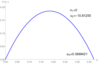
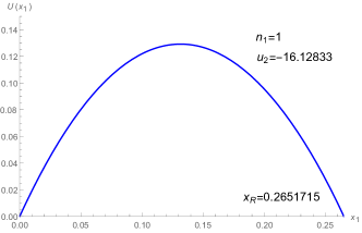
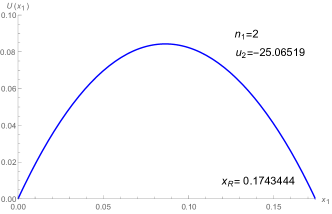
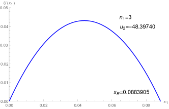
Figure 1: $(f_{0},f_{1},f_{2},f_{3},c_{1},c_{2},k)=(2,1,1,2,4,1,1)$ and $u_{1}=2$

First, $e^{-A(x_{1})}$ is positive definite within the domain $x_{1}\in(x_{L}=0,x_{R})$ for each case as can be seen in Figure 2. Since the numerical solution $U(x_{1})$, the linear function $f(x_{1})$, and $f_{1},f_{2}$ and $f_{3}$ are also all positive definite within the same domain, all the quantities in (3.33) are positive definite and therefore we have a positive-definite metric (3.1). Second, the domain of the $x_{1}$ coordinate is bounded so the corresponding global solution is compact. Third, $U^{\prime}(x_{R})=-2$ is satisfied for each $n_{1}$ with the chosen tunable parameters listed in Figure 1 and therefore we have $|U^{\prime}(x_{L})|=|U^{\prime}(x_{R})|=2$. This guarantees that the conical singularities at $x_{1}=x_{L},x_{R}$ can be removed provided that the period of the coordinate $\phi_{1}$ is chosen as $2\pi$.

Furthermore, these numerical solutions are continuously deformed under $n_{1}\to 0$ as demonstrated in the Figure 1. Such a smooth behavior makes these numerical solutions perfect candidates for mesonic twisted solutions compared to the polynomial solutions studied in section 3.4.1.

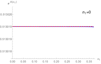
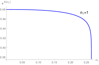
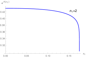
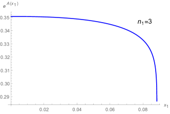
Figure 2: $(f_{0},f_{1},f_{2},f_{3},c_{1},c_{2},k)=(2,1,1,2,4,1,1)$ and $u_{1}=2$: Note that, in the upper-left panel for $n_{1}=0$, the numerical plot (blue) matches the constant value of $e^{A(x_{1})}$ from the exact quadratic polynomial solution $U(x_{1})=-{\frac{173}{32}}x_{1}(x_{1}-x_{R})$ (red, dashed).

Example 2

We find another numerical solution with different external parameters $(f_{0},f_{1},f_{2},f_{3},c_{1},c_{2},k)=({\frac{3}{2}},2,3,1,3,0,1)$, $u_{1}=2$, and $n_{1}=2$. The tunable parameter is chosen as $u_{2}=-21.32431$ for $U^{\prime}(x_{R})=-2$ as in Example 1 and the corresponding numerical solution is plotted in the left hand side of Figure 3. This set of external parameters satisfies the constraints for a quadratic polynomial solution studied in 3.4.1 to exist, namely $c_{2}=0$, $c_{1}^{2}>{\frac{4}{3f_{2}f_{3}}}$, and $k=1$. We have plotted the corresponding polynomial solution (3.32) with the negative sign in the right hand side of Figure 3. Figure 3 makes it explicit that the numerical solution obtained in this section are different from the polynomial solutions in a disconnected branch construction in section 3.4.1.

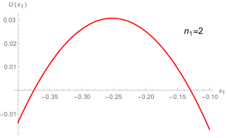
Figure 3: $(f_{0},f_{1},f_{2},f_{3},c_{1},c_{2},k)=({\frac{3}{2}},2,3,1,3,0,1)$ and $u_{2}=-21.32431$: the numerical solution(LHS) is distinguished from the polynomial solution(RHS).

4 Conclusions

In this manuscript we have conducted a partial classification of AdS₂ solutions in 11d supergravity. In the case where the M₉ manifold admits an SU(4)-structure the differential and algebraic conditions that the background needs to satisfy are given in (2.29a)-(2.30c). Let us briefly summarize the situation. Since an SU(4)-structure is canonically eight-dimensional, we find that the relevant data consists of a real 1-form $V$ strictly orthogonal to the SU(4)-structure in a way that generates M₉ metrically (see (2.18)). The $SU(4)$-structure itself is given by a $(1,1)$ form $J$ and a $(4,0)$ form $\Omega$. The 4-form flux of 11d supergravity is parametrixed in terms of a 2-form and a 4-form $(G_{2},G_{4})$, see (2.1). Thus, the necessary and sufficient conditions (2.29a)-(2.30c) are given in terms of $(V,J,\Omega)$ and the fluxes $(G_{2},G_{4})$.

From the classification point of view the truly new results in this manuscript pertain to the necessary and sufficient conditions for ${\cal N}=(1,0)$ supersymmetry (2.29a)-(2.30c). Our result refines the case of ${\cal N}=(2,0)$ susersymmetry which has been discussed previously in the literature albeit in a peculiar way through transgression [21]. Roughly, descending to the ${\cal N}=(2,0)$ case is equivalent to assuming that M₉ is a U(1) fibration over the M₈ base that is independent of U(1) coordinate, that is, the one-form $V$ in the general case becomes the one-form dual to the U(1) direction $\partial_{\psi}$.

It is worth pointing out that our approach, given its direct connection to [23], provides an embedding of a class of black-hole near horizons into a context general enough to describe the entire black-hole. Finding the full, interpolating, black holes remains an open problem but our work could easily become a first step in that direction. Having such full interpolating solutions from the near horizon to the asymptotically AdS₄ region would help clarify various aspects. For example, by evaluating its on-shell action one could potentially clarify the ${\cal I}$-extremizaiton procedure [41, 42, 43] in terms of an attractor mechanism in the bulk extending on previous related work along the lines of [45, 46, 47].

When specialized to the case of $Q^{1,1,1}$ our discussion provides a conceptual home for various solutions known in the literature and it allows us to present new solutions. We considered a series of generalizations culminating in a numerical analysis providing evidence for the existence of a solution with nontrivial baryonic as well as mesonic charges. We also found a peculiar solution which is disconnected from the $n_{1}=0$ branch, it would be opportune to track all the potential branches in the future.

It would be quite interesting to extend the classification of supersymmetric AdS₂ spaces allowing for more general M₉ spaces, that is, beyond the SU(4)-structure case. More physically, in this manuscript we elucidated the situations when the background can ultimately be understood as deformations of AdS${}_{4}\times$SE₇, that is, as backgrounds ultimately originating from M2 branes which naturally admit SU(4)-structure as we have discussed. It is quite relevant to extend our analysis in more detail to the class of supersymmetric solutions with AdS₂ factors pertaining to those arising from wrapped M5 branes. A prototypical class pertains to solutions where the M5 branes wrap a hyperbolic 3-manifold for which the dual field theory solution is well known (see, for example [48, 49, 7]). In the asymptotic AdS₄ regions the seven dimensional manifold is no longer a U(1) bundle over a Kahler-Einstein 6d manifold as in the case of M2 branes, rather it is a $S^{4}$ fibration over a hyperbolic 3-manifold [48, 50]. It is reasonable to expect that the AdS₂ classification of such solutions goes beyond the SU(4)-structure case treated here. Finally, let us point out another class that does not fit in our SU(4)-structure classificatory approach and that would be interesting to tackle - AdS₃ solutions in M-theory. Recall that AdS₃ can always be written as an AdS₂ foliation, therefore, a complete classification of AdS₂ solutions must include all AdS₃ solutions. However, in appendix B we proved the absence of AdS₃ solutions within the SU(4)-structure implying that to capture bubbling solutions [51, 52, 53] we need to generalize our work. We hope to return to these topics in the future.

Appendix A There are no AdS₂ solutions with Spin(7)-structure

In this Appendix we prove that there are no AdS₂ solutions in M-theory with internal space supporting a Spin(7)-structure globally.
 
Similar to an SU(4)-structure, a Spin(7)-structure in 9 dimensions can be defined in terms of two spinors, that are chiral when viewed in 8 dimensions. This time however these spinors should be equal. The canonical dimension of a Spin(7)-structure is 8, so M₉ will decompose as

$$ds^{2}(\text{M}_{9})=ds^{2}(\text{M}_{8})+U^{2},$$ (A.1)

with $\text{M}_{8}$ the manifold supporting the Spin(7)-structure and with $U$ a real 1-form that sits orthogonal to it.
 
We begin with spinor Ansatz

$$\epsilon=(\zeta_{+}+\zeta_{-})\otimes\chi,$$ (A.2)

for $\zeta_{\pm}$ and $\chi$ Majorana spinors on AdS₂ and M₉ respectively - $\pm$ labels 2d chirality as elsewhere. Let us without loss of generality fix the 8 dimensional chirality via the projections

$$\gamma_{1...8}\chi=\chi.$$ (A.3)

A Spin(7) structure in 9 dimensions is defined in terms of the 1-form $U$ and a real 4-form $\Psi$ with components given by

$$U_{a}=\chi^{{\dagger}}\gamma_{a}\chi,~{}~{}~{}~{}~{}\Psi_{a_{1}..a_{4}}=\chi^{{\dagger}}\gamma_{a_{1}..a_{4}}\chi$$ (A.4)

where $\star_{9}\Psi=U\wedge\Psi$. Using these definitions it is a simple matter to establish that the 11 dimensional supersymetric forms are given by

$$K =-re^{A}(e^{0}-e^{r}),$$ (A.5a)

$$\Omega =K\wedge U,$$ (A.5b)

$$\Sigma =K\wedge\Psi.$$ (A.5c)

Where $e^{0},e^{r}$ are the vielbein on warped AdS₂ given in (2.15). As such we now have $||K||^{2}=0$, so the Killing vector is null rather than time-like. However if we now attempt to solve the supersymmetry conditions $(K,\Omega,\Sigma)$ should obey, we find that we cannot. Specifically consider (2.13), this gives rise to

$$(r^{2}dt-dr)\wedge(e^{2A}G_{2}+d(e^{2A}U))+2re^{2A}U\wedge dt\wedge dr=0,$$ (A.6)

but the terms in this sum must vanish by themselves, and the second cannot be solved for a non zero spinor - hence there are no such solutions.

Appendix B No AdS₃ solutions within SU(4)-structure AdS₂ class

In this section we shall demonstrate that the class of AdS₂ solutions in section 2.3.2 is not exhaustive. We shall do so by proving that it contains no AdS₃ solutions which are known to exist in M-theory [54].
 
AdS₃ can be expressed as a foliation of AdS₂ over an interval as

$$ds^{2}(\text{AdS}_{3})=\cosh^{2}xds^{2}(\text{AdS}_{2})+dx^{2}.$$ (B.1)

As such a complete classification of AdS₂ solutions should contain all AdS₃ solutions as well. To find such solutions within section 2.3.2 , we must decompose the metric such that

$$e^{2A}ds^{2}(\text{AdS}_{2})+ds^{2}(\text{M}_{8})+V^{2}=e^{2A_{3}}\bigg{[}\cosh^{2}xds^{2}(\text{AdS}_{2})+dx^{2}\bigg{]}+ds^{2}(\tilde{\text{M}}_{8}),$$ (B.2)

and similarly for the fluxes. To achieve this we must clearly fix

$$e^{2A}=e^{2A_{3}}\,\cosh^{2}x.$$ (B.3)

In general the foliation direction $dx$ can lie partially along $V$ and partially along $\text{M}_{8}$, which supports the SU(4)-structure, as such we should decompose

$$V =\cos\zeta\,e^{A_{3}}dx+\sin\zeta\,k_{1},$$ (B.4)

$$J =(\cos\zeta\,k_{1}-\sin\zeta\,e^{A_{3}}dx)\wedge k_{2}+J_{3},$$ (B.5)

$$\Omega =(\cos\zeta\,k_{1}-\sin\zeta\,e^{A_{3}}dx+ik_{2})\wedge\Omega_{3},$$ (B.6)

where $J_{3},\Omega_{3}$ are the (1,1) and (3,0) forms defining an SU(3) structure in 6 dimensions, and $k_{1},k_{2}$ are two real 1-forms that together with the other six dimensions span $\tilde{\text{M}}_{8}$. The angle $\zeta$ is point dependent on $\tilde{\text{M}}_{8}$ and defines the alignment of $dx$. The above relations are analogous to a set introduced in [55] while discussing supersymmetric AdS₅ solutions in M-theory.
 
The decomposition (B.3)-(B.4) is sufficient to ensure an AdS₃ factor without loss of generality, provided the flux also respects the AdS₃ isometries. Unfortunately though, the possibility of AdS₃ dies as soon as one considers the supersymmety constraint (2.29a), which decomposes as

$$d(e^{A}J)=\cosh xd\big{(}e^{A_{3}}(J_{3}+\cos\zeta k_{1}\wedge k_{2})\big{)}+\cosh xdx\wedge d(e^{2A_{3}}\sin\zeta k_{2})+e^{A_{3}}\sinh xdx\wedge(J_{3}+\cos\zeta k_{1}\wedge k_{2}).$$

The issue is the final term in this expression which requires that $J_{3}+\cos\zeta k_{1}\wedge k_{2}=0$, since $J_{3},k_{1},k_{2}$ are by definition non zero and mutually orthogonal there is no way to solve this.
 
We have thus shown that there are no AdS₃ solutions contained in the class of section 2.3.2, and as such this class is clearly not the whole story for $\mathcal{N}=1$ AdS₂ in M-theory. Recall that there is a well-understood set of bubbling solutions of the form AdS${}_{3}\times S^{3}\times S^{3}\times\Sigma_{g}$ [51, 52, 53] that plays an important role in the AdS/CFT correspondence. There is also AdS₂ bubbling [56, 57].

Let us conclude this appendix by recalling that in [19] a solution containing AdS₂ was found exploiting a foliation of AdS₄ in the standard Freund-Rubin AdS${}_{4}\times$SE₇ solution. Note that realizing AdS₄ from AdS₂ requires one to allow $J_{3}$ and $\Omega$ to depend on $x$ above. We assume they do not since we are interested in AdS₃ with compact internal space, that is, AdS₃ that is not part of AdS₄ or some higher AdS factor.

Appendix C Killing spinor approach

The metric ansatz and the corresponding coframe are the same as (3.1) and (3.3). The 4-form ansatz is also the same as (3.4) with $G_{2}$ chosen explicitly as

$$G_{2}=H(x_{1})e^{4}\wedge e^{5}+\Sigma_{i=1}^{3}J_{i}(x_{1})e^{2i+4}\wedge e^{2i+5}+K_{1}(x_{1})e^{3}\wedge e^{6}.$$ (C.1)

Now we solve the Killing spinor equations, the 4-form Bianchi identity, and the 4-form equations of motion following the conventions of [23] (Einstein equations will automatically follows):

$$0 =\nabla_{\mu}\epsilon+{\frac{1}{288}}\left(\Gamma_{\mu}{}^{\nu_{1}\nu_{2}\nu_{3}\nu_{4}}-8\delta_{\mu}{}^{\nu_{1}}\Gamma^{\nu_{2}\nu_{3}\nu_{4}}\right)F_{\nu_{1}\nu_{2}\nu_{3}\nu_{4}}\epsilon,$$ (C.2)

$$0 =dF,$$ (C.3)

$$0 =d*F+{\frac{1}{2}}F\wedge F,$$ (C.4)

$$0 =R_{\mu\nu}-{\frac{1}{12}}\left(F_{\mu\nu_{1}\nu_{2}\nu_{3}}F_{\nu}{}^{\nu_{1}\nu_{2}\nu_{3}}-{\frac{1}{12}}g_{\mu\nu}F^{2}\right).$$ (C.5)

First, to solve the Killing spinor equations, we choose the following projections,

$$\Gamma^{1}\epsilon=\alpha\epsilon,\quad\Gamma^{23}\epsilon=\beta\epsilon,\quad\Gamma^{45}\epsilon=\gamma\epsilon,\quad\Gamma^{2i+4,2i+5}=\delta_{i}\epsilon~{}(i=1,2,3),$$ (C.6)

where $\alpha,\beta,\gamma,\delta_{i}\in\{\pm i\}$. Note that the above projections are given with respect to the coframe index. Under these projections, the Killing spinor equations (C.2) yield the differential conditions,

$$0 =\partial_{r}\epsilon-{\frac{1}{2r}}\epsilon,$$ (C.7a)

$$0 =(n\partial_{\psi}+n_{1}\partial_{\phi_{1}})\epsilon-{\frac{1}{2}}k\gamma\epsilon,$$ (C.7b)

$$0 =\partial_{x_{1}}\epsilon-{\frac{1}{2}}A^{\prime}(x_{1})\epsilon,$$ (C.7c)

$$0 =\partial_{\psi}\epsilon-{\frac{\delta_{2}}{2g_{2}}}\epsilon=\partial_{\psi}\epsilon-{\frac{\delta_{3}}{2g_{3}}}\epsilon,$$ (C.7d)

where $\partial_{\mu}\epsilon=0$ for $\mu=t,\theta,\phi,x_{i},\phi_{i}~{}(i=2,3)$. We can also derive the algebraic conditions,

$$e^{C(x_{1})} =-me^{A(x_{1})},$$ (C.8a)

$$m\beta =\delta_{2}/g_{2}=\delta_{3}/g_{3},$$ (C.8b)

$$H(x_{1}) =-\alpha\beta\gamma\,e^{2A(x_{1})}m\left(\delta_{1}{\frac{g^{\prime}(x_{1})}{f_{1}}}+\delta_{2}{\frac{g_{2}}{f_{2}}}+\delta_{3}{\frac{g_{3}}{f_{3}}}\right),$$ (C.8c)

$$J_{1}(x_{1}) =\alpha\left(-\beta\,e^{2A(x_{1})}m{\frac{g^{\prime}(x_{1})}{f_{1}}}+\delta_{1}e^{-A(x_{1})}\right),$$ (C.8d)

$$J_{i}(x_{1}) =\alpha\left(-\beta\,e^{2A(x_{1})}m{\frac{g_{i}}{f_{i}}}+\delta_{i}\,e^{-A(x_{1})}\right)\quad(i=2,3),$$ (C.8e)

$$K_{1}(x_{1}) =-3\alpha\beta\,e^{A(x_{1})/2}\sqrt{U(x_{1})}A^{\prime}(x_{1}),$$ (C.8f)

$$f(x_{1}) =f_{0}-n_{1}\gamma\delta_{1}x_{1},$$ (C.8g)

$$e^{3A(x_{1})} ={\frac{2f_{1}f_{2}f_{3}f(x_{1})}{2f_{1}f_{2}f_{3}(k+\gamma\delta_{1}n_{1}U^{\prime}(x_{1}))+f(x_{1})(2f_{1}(f_{2}+f_{3})-f_{2}f_{3}U^{\prime\prime}(x_{1}))}},$$ (C.8h)

$$g_{1}(x_{1}) =-{\frac{k}{mn_{1}}}\beta\gamma-{\frac{n}{n_{1}}}+{\frac{1}{2m}}\beta\left({\frac{n_{1}U(x_{1})}{f(x_{1})}}\gamma+U^{\prime}(x_{1})\delta_{1}\right),$$ (C.8i)

$$M_{ij}(x_{1}) =\gamma\delta_{i}\delta_{j}\delta_{k}|\epsilon_{ijk}|L_{k}(x_{1}),$$ (C.8j)

$$0 =\Sigma_{i=1}^{3}\delta_{i}L_{i}(x_{1}).$$ (C.8k)

where $m$ is a constant.

Provided that the Killing spinor equations (C.7) and (C.8) are satisfied, the 4-form Bianchi identity (C.3) yields

$$L_{1}(x_{1}) =c_{1}e^{2A(x_{1})},$$ (C.9a)

$$L_{2}(x_{1}) =\left(-{\frac{\delta_{1}c_{1}}{2\delta_{2}}}+{\frac{c_{2}}{f(x_{1})^{2}}}\right)e^{2A(x_{1})}.$$ (C.9b)

Finally, the 4-form equations of motion (C.4) yields a constraint on the projections and the 4th order ODE for $U(x_{1})$,

$$\alpha= ~{}\beta\gamma\delta_{1}\delta_{2}\delta_{3},$$ (C.10)

$$0= ~{}f_{1}^{2}f_{2}f_{3}(4c_{2}^{2}+f_{1}^{2}n_{1}^{4}U(x_{1})^{2})+2\gamma\delta_{1}f(x_{1})f_{1}^{3}f_{2}f_{3}n_{1}^{3}\left(U(x_{1})U^{\prime}(x_{1})\right)$$

$$+f(x_{1})^{2}f_{1}^{2}f_{2}f_{3}n_{1}^{2}\left(U^{\prime}(x_{1})^{2}+U(x_{1})U^{\prime\prime}(x_{1})\right)$$

$$+f(x_{1})^{3}f_{1}\left(-4f_{1}(f_{2}+f_{3})(k+\gamma\delta_{1}n_{1}U^{\prime}(x_{1}))+f_{2}f_{3}(2kU^{\prime\prime}(x_{1})+3\gamma\delta_{1}n_{1}(U(x_{1})U^{\prime\prime}(x_{1}))^{\prime})\right)$$

$$+f(x_{1})^{4}\left(-4f_{1}^{2}+3f_{1}^{2}f_{2}f_{3}c_{1}^{2}+2f_{1}(f_{2}+f_{3})U^{\prime\prime}(x_{1})-f_{2}f_{3}(U(x_{1})U^{\prime\prime\prime}(x_{1}))^{\prime}\right).$$ (C.11)

This expression coincides, of course, with (3.8) obtained in the main text using the geometric SU(4) structure conditions and the 4-form equation of motion.

References

- [1] F. Benini, K. Hristov and A. Zaffaroni, Black hole microstates in AdS4 from supersymmetric localization, JHEP 05 (2016) 054, [1511.04085].
- [2] F. Benini, K. Hristov and A. Zaffaroni, Exact microstate counting for dyonic black holes in AdS4, 1608.07294.
- [3] A. Cabo-Bizet, V. I. Giraldo-Rivera and L. A. Pando Zayas, Microstate counting of AdS4 hyperbolic black hole entropy via the topologically twisted index, JHEP 08 (2017) 023, [1701.07893].
- [4] F. Benini, H. Khachatryan and P. Milan, Black hole entropy in massive Type IIA, Class. Quant. Grav. 35 (2018) 035004, [1707.06886].
- [5] S. M. Hosseini, K. Hristov and A. Passias, Holographic microstate counting for AdS4 black holes in massive IIA supergravity, JHEP 10 (2017) 190, [1707.06884].
- [6] F. Azzurli, N. Bobev, P. M. Crichigno, V. S. Min and A. Zaffaroni, A universal counting of black hole microstates in AdS4, JHEP 02 (2018) 054, [1707.04257].
- [7] D. Gang, N. Kim and L. A. Pando Zayas, Precision Microstate Counting for the Entropy of Wrapped M5-branes, 1905.01559.
- [8] S. M. Hosseini, Black hole microstates and supersymmetric localization. PhD thesis, Milan Bicocca U., 2018-02. 1803.01863.
- [9] A. Zaffaroni, Lectures on AdS Black Holes, Holography and Localization, 2019. 1902.07176.
- [10] S. Choi, C. Hwang and S. Kim, Quantum vortices, M2-branes and black holes, 1908.02470.
- [11] J. Nian and L. A. Pando Zayas, Microscopic Entropy of Rotating Electrically Charged AdS4 Black Holes from Field Theory Localization, 1909.07943.
- [12] S. M. Hosseini and A. Zaffaroni, Large matrix models for 3d theories: twisted index, free energy and black holes, JHEP 08 (2016) 064, [1604.03122].
- [13] S. M. Hosseini and N. Mekareeya, Large topologically twisted index: necklace quivers, dualities, and Sasaki-Einstein spaces, JHEP 08 (2016) 089, [1604.03397].
- [14] S. L. Cacciatori and D. Klemm, Supersymmetric AdS(4) black holes and attractors, JHEP 01 (2010) 085, [0911.4926].
- [15] M. Cvetic, M. J. Duff, P. Hoxha, J. T. Liu, H. Lu, J. X. Lu et al., Embedding AdS black holes in ten-dimensions and eleven-dimensions, Nucl. Phys. B558 (1999) 96–126, [hep-th/9903214].
- [16] D. Cassani, P. Koerber and O. Varela, All homogeneous N=2 M-theory truncations with supersymmetric AdS4 vacua, JHEP 11 (2012) 173, [1208.1262].
- [17] N. Halmagyi, M. Petrini and A. Zaffaroni, BPS black holes in from M-theory, JHEP 08 (2013) 124, [1305.0730].
- [18] N. Halmagyi, Static BPS black holes in AdS4 with general dyonic charges, JHEP 03 (2015) 032, [1408.2831].
- [19] N. Kim and J.-D. Park, Comments on AdS(2) solutions of D=11 supergravity, JHEP 09 (2006) 041, [hep-th/0607093].
- [20] J. P. Gauntlett, N. Kim and D. Waldram, Supersymmetric AdS(3), AdS(2) and Bubble Solutions, JHEP 04 (2007) 005, [hep-th/0612253].
- [21] A. Donos, J. P. Gauntlett and N. Kim, AdS Solutions Through Transgression, JHEP 09 (2008) 021, [0807.4375].
- [22] A. Donos and J. P. Gauntlett, Supersymmetric quantum criticality supported by baryonic charges, JHEP 10 (2012) 120, [1208.1494].
- [23] J. P. Gauntlett and S. Pakis, The Geometry of D = 11 killing spinors, JHEP 04 (2003) 039, [hep-th/0212008].
- [24] J. P. Gauntlett, J. B. Gutowski and S. Pakis, The Geometry of D = 11 null Killing spinors, JHEP 12 (2003) 049, [hep-th/0311112].
- [25] O. A. P. Mac Conamhna and E. O Colgain, Supersymmetric wrapped membranes, AdS(2) spaces, and bubbling geometries, JHEP 03 (2007) 115, [hep-th/0612196].
- [26] S. Katmadas and A. Tomasiello, AdS4 black holes from M-theory, JHEP 12 (2015) 111, [1509.00474].
- [27] D. Prins, On flux vacua, -structures and generalised complex geometry. PhD thesis, Lyon, IPN, 2015. 1602.05415.
- [28] A. Legramandi, L. Martucci and A. Tomasiello, Timelike structures of ten-dimensional supersymmetry, JHEP 04 (2019) 109, [1810.08625].
- [29] J. P. Gauntlett, D. Martelli and D. Waldram, Superstrings with intrinsic torsion, Phys. Rev. D69 (2004) 086002, [hep-th/0302158].
- [30] O. Aharony, O. Bergman, D. L. Jafferis and J. Maldacena, N=6 superconformal Chern-Simons-matter theories, M2-branes and their gravity duals, JHEP 10 (2008) 091, [0806.1218].
- [31] D. Martelli and J. Sparks, Moduli spaces of Chern-Simons quiver gauge theories and AdS(4)/CFT(3), Phys. Rev. D78 (2008) 126005, [0808.0912].
- [32] A. Hanany and A. Zaffaroni, Tilings, Chern-Simons Theories and M2 Branes, JHEP 10 (2008) 111, [0808.1244].
- [33] S. Franco, I. R. Klebanov and D. Rodriguez-Gomez, M2-branes on Orbifolds of the Cone over Q**1,1,1, JHEP 08 (2009) 033, [0903.3231].
- [34] F. Benini, C. Closset and S. Cremonesi, Chiral flavors and M2-branes at toric CY4 singularities, JHEP 02 (2010) 036, [0911.4127].
- [35] S. Cheon, H. Kim and N. Kim, Calculating the partition function of N=2 Gauge theories on and AdS/CFT correspondence, JHEP 05 (2011) 134, [1102.5565].
- [36] D. Martelli and J. Sparks, AdS(40 / CFT(3) duals from M2-branes at hypersurface singularities and their deformations, JHEP 12 (2009) 017, [0909.2036].
- [37] C. P. Herzog, I. R. Klebanov, S. S. Pufu and T. Tesileanu, Multi-Matrix Models and Tri-Sasaki Einstein Spaces, Phys. Rev. D83 (2011) 046001, [1011.5487].
- [38] A. Amariti, M. Fazzi, N. Mekareeya and A. Nedelin, New 3d SCFT’s with scaling, 1903.02586.
- [39] D. Jain and A. Ray, 3d Chern-Simons quivers, Phys. Rev. D100 (2019) 046007, [1902.10498].
- [40] D. Jain, Twisted Indices of more 3d Quivers, 1908.03035.
- [41] J. P. Gauntlett, D. Martelli and J. Sparks, Toric geometry and the dual of -extremization, JHEP 06 (2019) 140, [1904.04282].
- [42] S. M. Hosseini and A. Zaffaroni, Geometry of -extremization and black holes microstates, 1904.04269.
- [43] H. Kim and N. Kim, Black holes with baryonic charge and -extremization, 1904.05344.
- [44] C. P. Herzog and I. R. Klebanov, Gravity duals of fractional branes in various dimensions, Phys. Rev. D63 (2001) 126005, [hep-th/0101020].
- [45] A. Cabo-Bizet, U. Kol, L. A. Pando Zayas, I. Papadimitriou and V. Rathee, Entropy functional and the holographic attractor mechanism, JHEP 05 (2018) 155, [1712.01849].
- [46] N. Halmagyi and S. Lal, On the on-shell: the action of AdS4 black holes, JHEP 03 (2018) 146, [1710.09580].
- [47] P. Benetti Genolini, J. M. Pérez Ipiña and J. Sparks, Localization of the action in AdS/CFT, 1906.11249.
- [48] D. Gang, N. Kim and S. Lee, Holography of 3d-3d correspondence at Large N, JHEP 04 (2015) 091, [1409.6206].
- [49] D. Gang and N. Kim, Large twisted partition functions in 3d-3d correspondence and Holography, Phys. Rev. D99 (2019) 021901, [1808.02797].
- [50] I. Bah, M. Gabella and N. Halmagyi, BPS M5-branes as Defects for the 3d-3d Correspondence, JHEP 11 (2014) 112, [1407.0403].
- [51] H. Lin, O. Lunin and J. M. Maldacena, Bubbling AdS space and 1/2 BPS geometries, JHEP 10 (2004) 025, [hep-th/0409174].
- [52] O. Lunin, 1/2-BPS states in M theory and defects in the dual CFTs, JHEP 10 (2007) 014, [0704.3442].
- [53] E. D’Hoker, J. Estes, M. Gutperle and D. Krym, Exact Half-BPS Flux Solutions in M-theory. I: Local Solutions, JHEP 08 (2008) 028, [0806.0605].
- [54] D. Martelli and J. Sparks, G structures, fluxes and calibrations in M theory, Phys. Rev. D68 (2003) 085014, [hep-th/0306225].
- [55] J. P. Gauntlett, D. Martelli, J. Sparks and D. Waldram, Supersymmetric AdS(5) solutions of M theory, Class. Quant. Grav. 21 (2004) 4335–4366, [hep-th/0402153].
- [56] I. Bena, P. Heidmann and D. Turton, AdS2 holography: mind the cap, JHEP 12 (2018) 028, [1806.02834].
- [57] Y.-Z. Li, S.-L. Li and H. Lu, Exact Embeddings of JT Gravity in Strings and M-theory, Eur. Phys. J. C78 (2018) 791, [1804.09742].