Pro-Cam SSfM: Projector-Camera System
for Structure and Spectral Reflectance from Motion

Abstract

In this paper, we propose a novel projector-camera system for practical and low-cost acquisition of a dense object 3D model with the spectral reflectance property. In our system, we use a standard RGB camera and leverage an off-the-shelf projector as active illumination for both the 3D reconstruction and the spectral reflectance estimation. We first reconstruct the 3D points while estimating the poses of the camera and the projector, which are alternately moved around the object, by combining multi-view structured light and structure-from-motion (SfM) techniques. We then exploit the projector for multispectral imaging and estimate the spectral reflectance of each 3D point based on a novel spectral reflectance estimation model considering the geometric relationship between the reconstructed 3D points and the estimated projector positions. Experimental results on several real objects demonstrate that our system can precisely acquire a dense 3D model with the full spectral reflectance property using off-the-shelf devices.

1 Introduction

The nature of an object is typically represented by two properties: geometric and photometric properties. The geometric property is determined by the 3D structure of the object, while the photometric property is determined by how the incident light is reflected at each 3D point of the object surface. Among various photometric parameters, spectral reflectance is one of the most fundamental physical quantities, which defines the amount of reflected light over that of the incident light at each wavelength. In this work, our aim is to acquire the spectral 3D information of an object using low-cost off-the-shelf devices (see Fig. 1). Practical and low-cost acquisition of the spectral 3D information has many potential applications in fields such as cultural heritage [9, 28], plant modeling [7, 31], spectral rendering [12], and multimedia [33].

3D reconstruction is a very active research area in computer vision. Structure from motion (SfM) [43, 46], multi-view stereo [15, 44], and structured light [14, 16, 17, 30, 42] are common approaches for the 3D shape acquisition. However, they usually focus on the geometric reconstruction. Although some recent methods combine the geometric and the photometric reconstruction [26, 34, 35], they still focus on the estimation of RGB albedo, which is dependent on the camera RGB sensitivity and not an inherent property of the object unlike the spectral reflectance.

Multispectral imaging is another active research area. Various hardware-based systems [6, 8, 10, 18, 36, 40, 48] and software-based methods [2, 5, 13, 22, 38, 45] have been proposed for recovering scene’s spectral reflectance. However, they usually assume a single-viewpoint input image and do not consider the geometric relationship between the object surface and the light source, only achieving scene and viewpoint-dependent spectral recovery, where shading or shadow is “baked in” the recovered spectral reflectance.

Some systems have also been proposed for spectral 3D acquisition [19, 21, 27, 29, 39, 49]. However, they rely on a dedicated setup using a multispectral camera [27, 39, 49] or a multispectral light source [19, 21, 29], which makes the system impractical and expensive for most users.

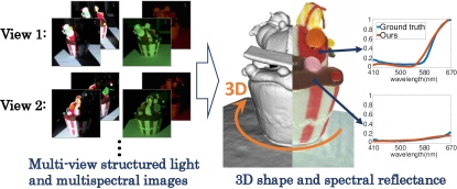
Figure 1: From multi-view structured light and multispectral images captured using an alternately moved projector and camera, our system can reconstruct a dense object 3D model having the spectral reflectance property for each 3D point.

In this paper, we propose a novel projector-camera system, named Pro-Cam SSfM, for structure and spectral reflectance from motion. In Pro-Cam SSfM, we use a standard RGB camera and leverage an off-the-shelf projector for two roles: structured light and multispectral imaging. For the data acquisition, structured light patterns (for geometric observations) and uniform color illuminations (for multispectral observations) are sequentially projected onto the object surface while alternately moving the camera and the projector positions around the object. Using the multi-view structured light data, we first reconstruct the 3D points while estimating the poses of all moved cameras and projectors. Using the multi-view multispectral data, we then estimate the spectral reflectance of each 3D point considering the geometric relationship between the reconstructed 3D points and the estimated projector positions.

Technical contributions of this work are listed as below.

1. We propose an extended self-calibrating multi-view structured light method, where we include the moved projectors for feature correspondences and pose estimation to realize denser 3D reconstruction. The estimated projector positions are further exploited for the following spectral reflectance estimation.

2. We propose a novel spectral reflectance estimation model by incorporating the geometric relationship between the reconstructed 3D points and the estimated projector positions into the cost optimization. Our model leads accurate estimation of the inherent spectral reflectance of each 3D point while eliminating the baked-in effect of the shading and the shadow.

3. By integrating the above key techniques into one system, we propose Pro-Cam SSfM, a novel projector-camera system for practical and low-cost spectral 3D acquisition. We experimentally demonstrate that Pro-Cam SSfM can precisely reconstruct a dense object 3D model with the spectral reflectance property. To the best of our knowledge, Pro-Cam SSfM is the first spectral 3D acquisition system using off-the-shelf devices.

2 Related Work

Structured light systems: Structured light is a well-adopted technique to accurately reconstruct the 3D points irrespective of surface textures by projecting structured light patterns [4, 17, 42, 47]. While structured light methods are generally based on a pre-calibrated projector-camera system, some multi-view structured light methods [14, 16, 30] have realized self-calibrating reconstruction of the 3D points. The key of these methods is that the structured light patterns projected by one fixed projector is captured from more than two camera viewpoints having viewing angle overlaps, so that feature matching and tracking can be made to connect all projectors and cameras. This setup can be realized by simultaneously using multiple projectors and cameras [14, 16] or alternately moving a projector and a camera [30].

In Pro-Cam SSfM, we extend the method [30] for realizing denser 3D reconstruction, as detailed in Section 3.2. We also exploit the estimated projector positions for modeling the spectral reflectance, while existing methods [14, 16, 30] only focus on the geometric reconstruction.

Multispectral imaging systems: Existing hardware-based [6, 8, 10, 18, 36, 48, 40] or software-based [2, 5, 13, 22, 38, 45] multispectral imaging systems commonly apply a single-viewpoint image-based spectral reflectance estimation method ignoring scene’s or object’s geometric information. This means that they only achieve scene-dependent spectral reflectance estimation, where the viewpoint and scene-dependent shading or shadow is baked in the estimated spectral reflectance.

In Pro-Cam SSfM, we use an off-the-shelf RGB camera and projector for multispectral imaging. Although this setup is the same as [18], we propose a novel spectral reflectance estimation model for recovering the object’s inherent spectral reflectance considering the geometric information that can be obtained at the 3D reconstruction step.

Spectral 3D acquisition systems: Existing systems for spectral 3D acquisition are roughly classified into photometric stereo-based [29, 39], SfM and multi-view stereo-based [21, 49], and active lighting or scanner-based [19, 27] systems. The photometric stereo-based systems [29, 39] can acquire dense surface normals for every pixels of the single-view image. However, they have a main limitation that the light positions should be calibrated. The SfM and multi-view stereo-based systems [21, 49] enable self-calibrating 3D reconstruction using multi-view images. However, they only can provide a sparse point cloud especially for a texture-less object. The active lighting or scanner-based systems [19, 27] can provide an accurate and dense 3D model based on the active sensing. However, they require burdensome calibration of the entire system. Furthermore, all of the above-mentioned systems rely on a dedicated setup using a multispectral camera [27, 39, 49] or a multispectral light source [19, 21, 29] for achieving multispectral imaging capability. Those limitations make the existing system impractical and expensive for most users, narrowing the range of applications.

Pro-Cam SSfM overcomes those limitations because (i) it uses a low-cost off-the-shelf camera and projector, (ii) it does not require geometric calibration, and (iii) it generates a dense 3D model based on the structured light.

3 Proposed Pro-Cam SSfM

Pro-Cam SSfM consists of three parts: data acquisition, self-calibrating 3D reconstruction, and spectral reflectance estimation. Each part is detailed below.

3.1 Data acquisition

Figure 2 illustrates the data acquisition procedure of Pro-Cam SSfM. We use an off-the-shelf projector as active illumination and a standard RGB camera as the imaging device to capture the object illuminated by the projector. As shown in Fig. 2(a), the projector is used to project a sequence of structured light patterns and uniform color illuminations to acquire geometric and photometric observations. As the structured light patterns, we use the binary gray code [17, 42]. As the uniform color illuminations, we use the seven illuminations: red, green, blue, cyan, magenta, yellow, and white illuminations, which are generated using the binary combinations of the RGB primaries as (R,G,B) = (1,0,0), (0,1,0), (0,0,1), (0,1,1), (1,0,1), (1,1,0), (1,1,1), respectively. The sequence of active projections are effectively exploited in the 3D reconstruction and the spectral reflectance estimation.

To scan the whole object, we follow the data acquisition procedure of [30]. The data acquisition starts with initial projector and camera positions (e.g., position 1 in Fig. 2(b)). Then, the camera and the projector are alternately moved around the object (e.g., motion 1, motion 2, and so on, in Fig. 2(b)). This acquisition procedure enables to connect the structured light codes (i.e., feature points) between successive projectors and cameras. All connected feature points using all projector and camera positions are used as correspondences for the SfM pipeline, which enables self-calibrating reconstruction of the 3D points while estimating the poses of all moved projectors and cameras.

3.2 Self-calibrating 3D reconstruction

Given the structured light encoded images, we first perform self-calibrating reconstruction of the 3D points while estimating the poses of all moved cameras and projectors. This is performed by extending [30] as below.

3.2.1 Feature correspondence

By projecting gray code patterns as shown in Fig. 2(a), the projector can add “features” on object surfaces. Those features have different codes whose number is the same as the projector resolution. By decoding the code for each pixel and calculating the center position of the pixels having the same code, we can obtain “features” at sub-pixel accuracy positions in each image.

The feature correspondences for camera-projector pairs (e.g., camera1-projector1 and camera2-projector1 pairs in Fig. 2(b)) and camera-camera pairs (e.g., camera1-camera2 pair) sharing the same projector code are obvious. The features from different projectors can be connected using a common camera (e.g., camera2 for projector1 and projector2), i.e., the features from different projectors are regarded as identical, if their positions are close enough (less than 0.5 pixels in our experiments). Once they are connected, correspondences can be made for all combinations of cameras and projectors (e.g., even correspondence for a projector-projector pair can be made). In contrast to the fact that the method [30] only uses the correspondences of all camera-camera pairs, we use all correspondences including projectors, which results in denser 3D points as shown in Fig. 5.

(a) Projected illuminations
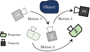
(b) Data acquisition procedure

Figure 2: Data acquisition procedure of Pro-Cam SSfM. (a) The projector projects a sequence of structured light patterns (gray code) and uniform color illuminations to acquire geometric and photometric observations. (b) The camera and the projector are alternately moved around the object, so that the structured light codes can be connected among all camera and projector positions.

3.2.2 3D point and projector-camera pose estimation

The set of all obtained correspondences is then fed into a standard SfM pipeline [43, 46] to estimate the 3D points, the projector poses, and the camera poses. In the SfM pipeline, we modify the bundle adjustment formulation [32] so as to minimize the following weighted reprojection errors.

$$E=\sum_{i}\sum_{k}w_{i}\|\bm{x}_{k,i}-H_{i}(\bm{p}_{k})\|^{2},$$ (1)

where $\bm{p}_{k}$ is the 3D coordinate of point $k$, $\bm{x}_{k,i}$ is the corresponding pixel coordinates in $i$-th viewpoint (camera or projector), and $H_{i}(\bm{p})$ is a function that projects the 3D point to $i$-th viewpoint (camera or projector) using intrinsic and extrinsic parameters for each projector and each camera. In Eq. (1), we set a larger weight to impose higher penalties for the reprojection errors of the projector as

$$w_{i}=\begin{cases}1,&\text{if viewpoint $i$ is a camera}\\ w_{p},&\text{if viewpoint $i$ is a projector}\end{cases},$$ (2)

where $w_{p}>1$, because it can be regarded that “feature” positions of projectors have almost no errors. Through the bundle adjustment, 3D points and whole system parameters, including projector and camera positions and intrinsic parameters for both projectors and cameras are estimated without any pre-calibration.

3.3 Spectral reflectance estimation

Given the estimated 3D points, projector positions, and camera poses, we next estimate the spectral reflectance of each 3D point. For this purpose, we use multispectral images captured under the uniform color illuminations. In what follows, we first introduce our proposed rendering model and then explain cost optimization to estimate the spectral reflectance using multi-view multispectral images.

3.3.1 Rendering model

We here introduce our rendering model for each 3D point using a single projector-camera pair. Suppose the object surface is modeled by Lambertian reflectance and the camera response is linear, the camera’s pixel intensity $y$ for $k$-th 3D point captured by $m$-th camera channel and $n$-th projected illumination is modeled as

$$y_{k,m,n}(\bm{x}_{k})=s_{k}\int_{\Omega_{\lambda}}c_{m}(\lambda)l_{n}(\lambda)r(\bm{p}_{k},\lambda)d\lambda,$$ (3)

where $\bm{x}_{k}$ is the projected pixel coordinate for $k$-th point, $r(\bm{p}_{k},\lambda)$ is the spectral reflectance of $k$-th point, $l_{n}(\lambda)$ is the spectral power distribution of $n$-th projected illumination, $c_{m}(\lambda)$ is the camera spectral sensitivity of $m$-th channel, $s_{k}$ is the shading factor for $k$-th point, and $\Omega_{\lambda}$ is the target wavelength range. In practice, the continuous wavelength domain is discretized to $N_{\lambda}$ dimension (typically, sampled at every 10nm from 400nm to 700nm, i.e., $N_{\lambda}$=31). Suppose the camera has three (i.e., RGB) channels and $N_{l}$ illuminations are projected, the observed multispectral intensity vector for $k$-th point $\bm{y}_{k}\in\mathbb{R}^{3N_{l}}$ can be expressed as

$$\bm{y}_{k}=s_{k}\bm{C}^{T}\bm{L}\bm{r}_{k},$$ (4)

where $\bm{r}_{k}\in\mathbb{R}^{N_{\lambda}}$ represents the spectral reflectance, $\bm{L}=[\bm{L}_{1};\cdots;\bm{L}_{N_{l}}]\in\mathbb{R}^{N_{l}N_{\lambda}\times N_{\lambda}}$ is the illumination matrix, where $\bm{L}_{n}\in\mathbb{R}^{N_{\lambda}\times N_{\lambda}}$ is the $n$-th diagonal illumination matrix, and $\bm{C}^{T}=blockdiag(\bm{C}_{rgb}^{T},\cdots,\bm{C}_{rgb}^{T})\in\mathbb{R}^{3N_{l}\times N_{l}N_{\lambda}}$ is the block diagonal matrix, where $\bm{C}_{rgb}^{T}\in\mathbb{R}^{3\times N_{\lambda}}$ is the camera sensitivity matrix. In this work, we assume that the spectral power distributions of the projected illuminations and the camera sensitivity (i.e., $\bm{C}^{T}$ and $\bm{L}$) are known or preliminarily estimated (e.g., by [23, 48]).

3.3.2 Spectral reflectance model

It is known that the spectral reflectance of natural objects is well represented by a small number of basis functions [41]. Based on this observation, we adopt a widely used basis model [18, 40], where the spectral reflectance is modeled as

$$\bm{r}_{k}=\bm{B}\bm{\alpha}_{k},$$ (5)

where $\bm{B}\in\mathbb{R}^{N_{\lambda}\times N_{b}}$ is the basis matrix, where $N_{b}$ is the number of basis functions, and $\bm{\alpha}_{k}\in\mathbb{R}^{N_{b}}$ is the coefficient vector. The basis model can reduce the number of parameters (since $N_{b}<N_{\lambda}$) for spectral reflectance estimation. Using the basis model, Eq. (4) is rewritten as

$$\bm{y}_{k}=s_{k}\bm{C}^{T}\bm{L}\bm{B}\bm{\alpha}_{k}.$$ (6)

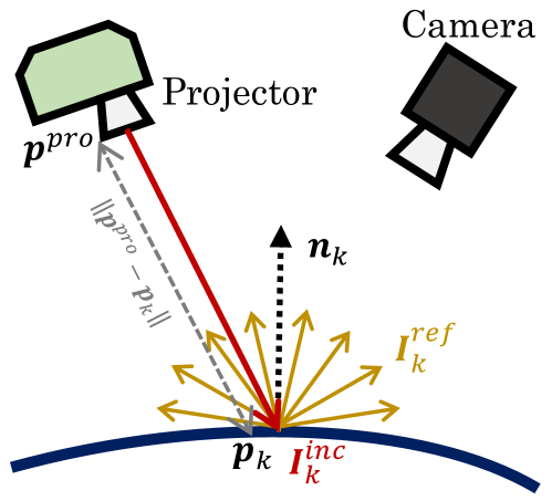
Figure 3: Geometric relationship between the projector $\bm{p}^{pro}$ and the 3D point $\bm{p}_{k}$ to calculate the shading factor. We assume that the point has Lambertian reflectance and the projected illumination follows the inverse-square law.

3.3.3 Shading model

Different from common single-view image-based methods (e.g., [18, 19, 48, 40]), we take the shading factor into account for spectral reflectance estimation, which results in more accurate model and estimation. Figure 3 illustrates the relationship between the projector position $\bm{p}^{pro}$, $k$-th 3D point $\bm{p}_{k}$, and the point normal $\bm{n}_{k}$ (which can be calculated using [20]). Since the shading factor is wavelength independent and determined by the geometric relationship between the projector and the 3D point (under the Lambertian reflectance assumption), we rewrite the illumination power as $l(\lambda)=l$ in the following derivation. Then, the shading factor at $k$-th point is modeled as

$$s_{k}=I_{k}^{ref}/l,$$ (7)

where $I_{k}^{ref}$ is the irradiance of the reflected light incoming to the camera. In our model, the shading factor determines how much the amount of the projected illumination reaches the camera, irrespective of the spectral reflectance. If we assume Lambartian reflectance, $I_{k}^{ref}$ is independent of the camera position and expressed as

$$I^{ref}_{k}=I^{inc}_{k}\times\frac{\bm{p}^{pro}-\bm{p}_{k}}{\|\bm{p}^{pro}-\bm{p}_{k}\|}\cdot\bm{n}_{k},$$ (8)

where $I^{inc}_{k}$ is the irradiance of the incident light at $k$-th point and $(\bm{p}^{pro}-\bm{p}_{k})/\|\bm{p}^{pro}-\bm{p}_{k}\|\cdot\bm{n}_{k}$ represents the inner product of the normalized lighting vector and the point normal (see Fig. 3). Based on the near-by light model and the inverse-square law, $I^{inc}_{k}$ is inversely proportional to the square of the distance from the projector to the 3D point as

$$I^{inc}_{k}=\frac{l}{\|\bm{p}^{pro}-\bm{p}_{k}\|^{2}}.$$ (9)

If we assume that the ambient light is negligible and omit interreflection from the model, the shading factor is modeled from Eqs. (7)–(9) as

$$s_{k}=\frac{\bm{p}^{pro}-\bm{p}_{k}}{\|\bm{p}^{pro}-\bm{p}_{k}\|^{3}}\cdot\bm{n}_{k}.$$ (10)

Based on this model, the shading factor can be calculated from the 3D point, the point normal, and the projector position that we have already obtained by the self-calibrating 3D reconstruction. The final rendering model is derived by substituting Eq. (10) into Eq. (6).

3.3.4 Visibility calculation

To estimate the spectral reflectance using multi-view images, we need to calculate the visibility of each 3D point. For this purpose, the object surface is reconstructed using Poisson surface reconstruction [24, 25]. Then, for each projector-camera pair, a set of 3D points that are visible from both the camera and the projector is calculated. By calculating the visibility, we discount the effects of cast shadows for spectral reflectance estimation.

3.3.5 Cost optimization

Using the rendering model of Eq. (6), we solve an optimization problem to estimate the spectral reflectance of each 3D point from multi-view images obtained from all projector-camera pairs. The cost function is defined as

$$\arg\min_{\bm{\alpha}_{k}}~{}E_{ren}(\bm{\alpha}_{k})+\gamma E_{ssm}(\bm{\alpha}_{k}),$$ (11)

where $E_{ren}$ is the rendering term and expressed as

$$E_{ren}(\bm{\alpha}_{k})=\sum_{c\in\mathcal{V}(k)}\frac{\|{\bm{y}}_{k,c}^{obs}-\bm{y}_{k,c}(\bm{\alpha}_{k})\|^{2}}{|\mathcal{V}(k)|},$$ (12)

where ${\bm{y}}_{k,c}^{obs}\in\mathbb{R}^{3N_{l}}$ is the observed multispectral intensity vector obtained from $c$-th projector-camera pair, ${\bm{y}}_{k,c}(\bm{\alpha}_{k})$ is the estimated intensity vector based on the rendering model, and $\mathcal{V}(k)$ is the visible set for $k$-th point. This term evaluates the data fidelity between the observed and the rendered intensities. $E_{ssm}$ is a commonly used spectral smoothness term [18, 48, 40], which is defined by

$$E_{ssm}(\bm{\alpha}_{k})=\bm{D}\bm{B}\bm{\alpha}_{k},$$ (13)

where $\bm{D}\in\mathbb{R}^{N_{\lambda}\times N_{\lambda}}$ is the operation matrix to calculate the second-order derivative [40]. This term evaluates the smoothness of the estimated spectral reflectance. The balance of $E_{ren}$ and $E_{ssm}$ is determined by the parameter $\gamma$.

Camera sensitivity	Red	Green	Blue
Cyan	Magenta	Yellow	White

Figure 4: Camera spectral sensitivity and spectral power distribution of each uniform color illumination.

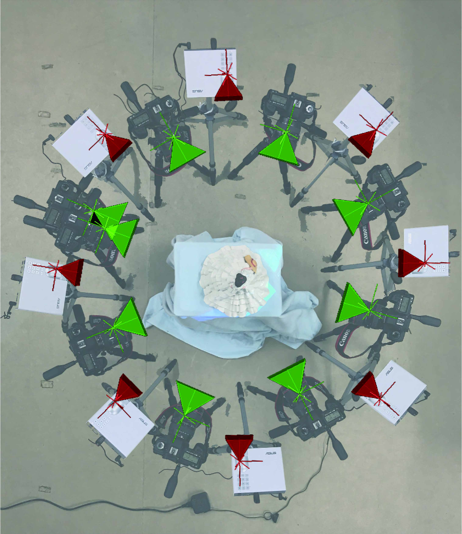
(a) Synthesized top view

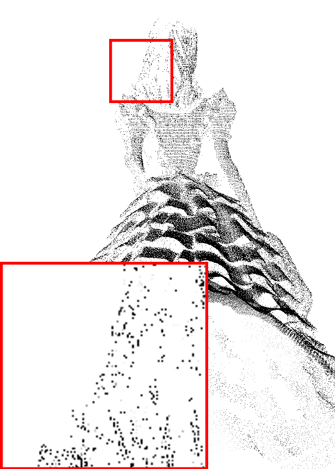
(b) Method [30]

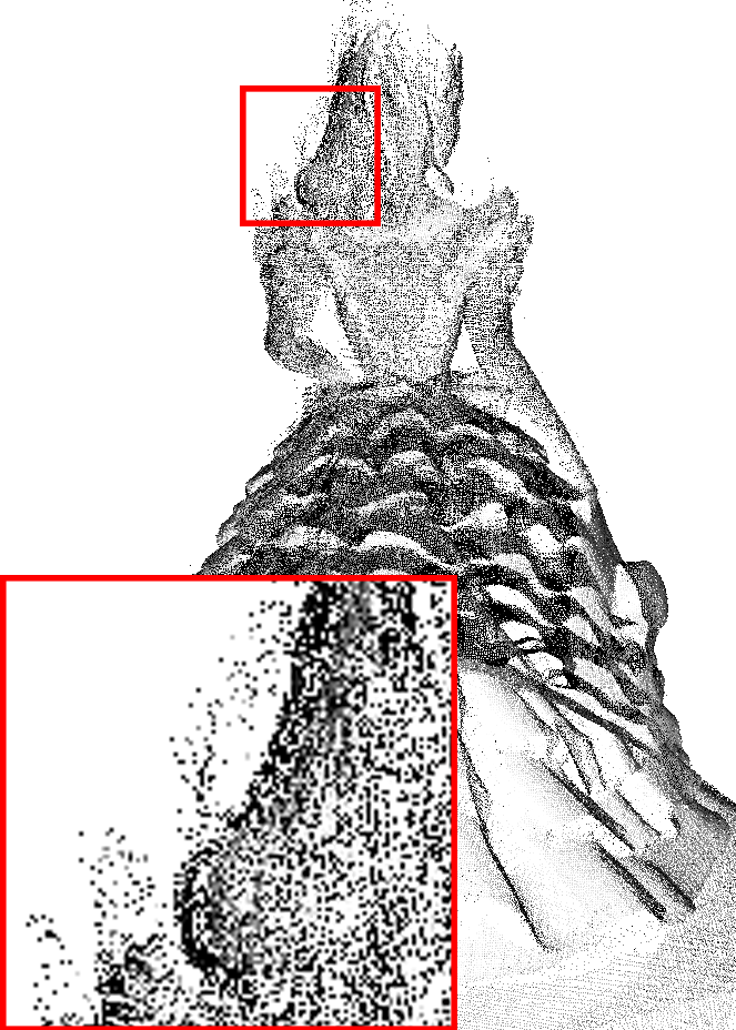
(c) Ours w/o weight

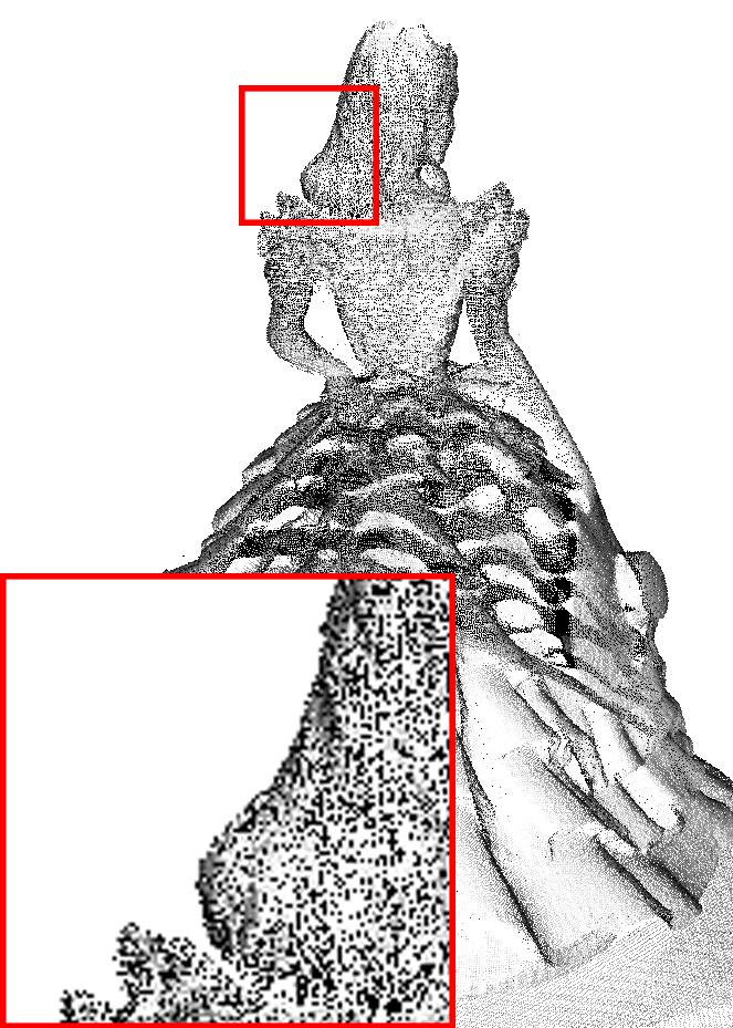
(d) Our method

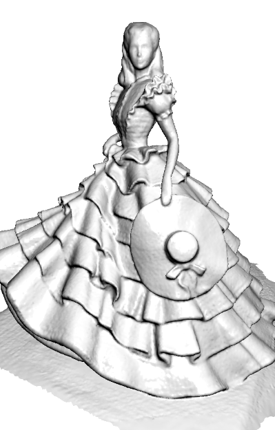
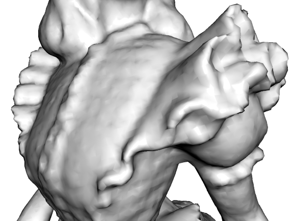
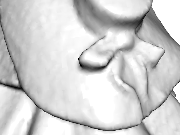
(e) 3D surface result of our method

Figure 5: 3D reconstruction results: (a) The synthesized top-view image to schematically show the layout of the moved projector and camera positions. The estimated projector and camera positions are overlaid as the red and the green triangular pyramids; (d) Our method generates 210,523 points, while (b) the method [30] generates 105,915 points; (c) The result of our method without the bundle adjustment weight, which leads to reconstruction errors; (e) The 3D surface result reconstructed from the 3D points (d).

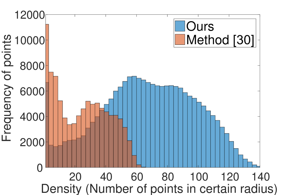
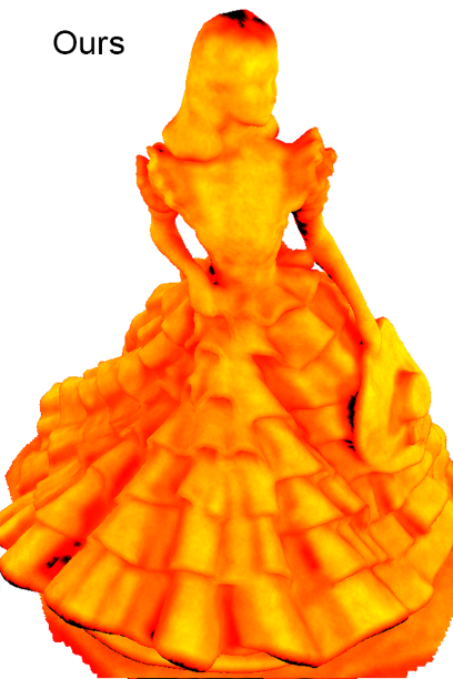
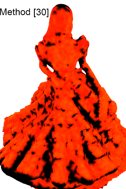
Figure 6: Evaluation of 3D point cloud density. Left: The density histogram of reconstructed points. Right: Visualization of its spacial distribution.

4 Experimental Results

4.1 Setup and implementation details

We used an ASUS P3B projector and a Canon EOS 5D Mark-II digital camera. The sequence of the structured light patterns was captured using a video format with 1920$\times$1080 resolution, while the color illuminations were captured using a RAW format, which has a linear camera response, with a higher resolution. The RAW images were then resized to have the same resolution with the video format. As shown in Fig. 4, the camera spectral sensitivity of Canon EOS 5D Mark-II was obtained from the camera sensitivity database [23] and the spectral power distributions of the color illuminations were measured using a spectrometer.

For the 3D reconstruction, we used Colmap [43] to run the SfM pipeline and Poisson surface reconstruction [24, 25], which is integrated with Meshlab [11], to visualize the obtained 3D model. For the spectral reflectance estimation, we set the target wavelength range as 410nm to 670nm with every 10nm intervals because the used projector illuminations only have the spectral power within this range. We used eight basis functions, which were calculated using the spectral reflectance data of 1269 Munsell color chips [1] by principal component analysis. The spectral smoothness weight in Eq. (11) was determined by an empirical manner and set as $\gamma=0.06$ for the intensity range [0,1]. The C++ Ceres solver [3] was used to solve the non-linear optimization problem of Eq. (11).

4.2 3D reconstruction results

Figure 5 shows the self-calibrating 3D reconstruction results of a clay sculpture with roughly 30 centimeter height. To schematically show the layout of the moved projector and camera positions, we show a synthesized top-view image of Fig. 5(a). The estimated projected and camera positions by our method are overlaid as the red and the green triangular pyramids using a manually aligned scale. It is demonstrated that the projector and the camera positions are correctly estimated by our method.

Figure 5(b) and 5(d) show the 3D point cloud results of the method [30] and our method, which were reconstructed using exactly the same setup and images. The difference is that our method uses both camera and projector images for SfM computation, while the method [30] uses only camera images. Our method can reconstruct the 210,523 points, which are almost double of the 105,915 points reconstructed by the method [30]. To quantitatively evaluate the point cloud density, we counted the number of reconstructed 3D points within a certain radius from each point. Figure 6 shows the density histogram of reconstructed points (left) and the visualization of its spacial distribution (right), where our method achieves much denser 3D reconstruction.

Another improvement can be achieved by introducing the weight of Eq. (1) for bundle adjustment, which poses larger penalties to the projector’s reprojection errors. In our experiments, we set as $w_{p}$ = 100, though a larger value more than 10 does not make a big difference. We experimentally observed that the estimation of the projector’s positions and internal parameters often fails if we do not use the weight, which leads to reconstruction errors as can be seen in Fig. 5(c). Figure 5(e) shows the final reconstructed surface result for our method, where the detail structures of the sculpture are precisely reconstructed.

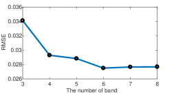
Figure 7: RMSE for the 24 patches of the colorchart when using the selected best band set for each number of spectral bands.

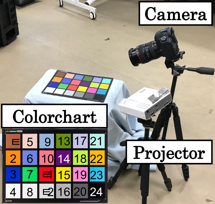
(a) Experimental setup

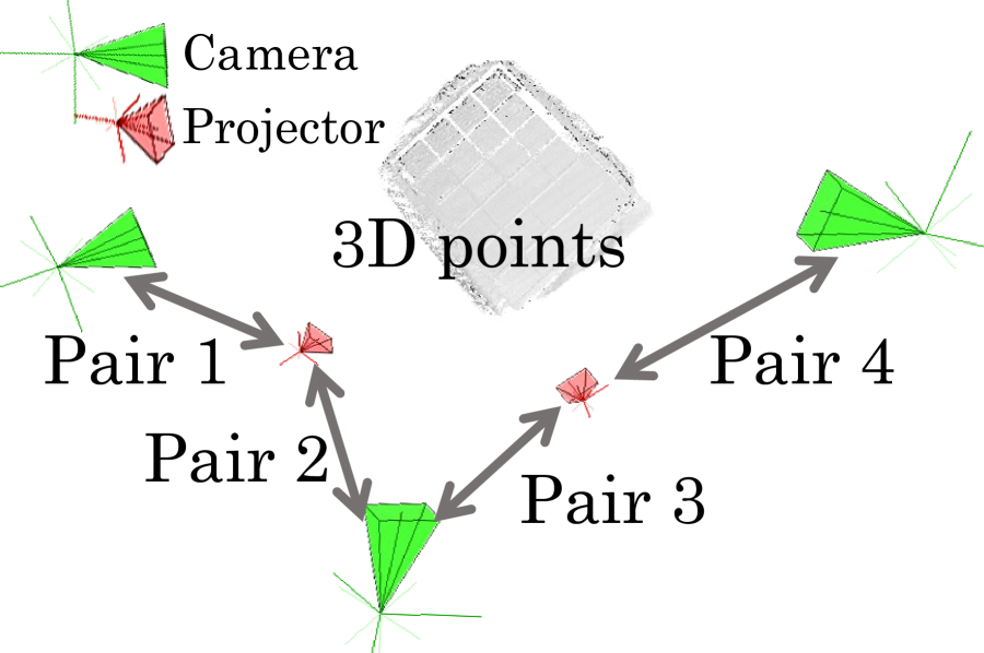
(b) Estimated 3D points and projector and camera poses

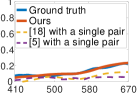
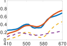
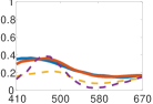
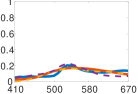
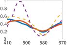
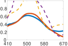
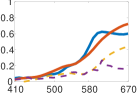
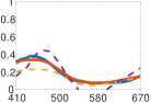
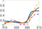
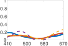
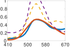
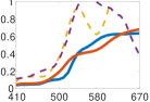
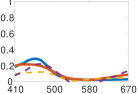
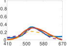
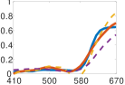
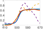
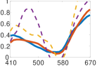
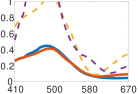
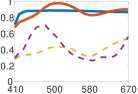
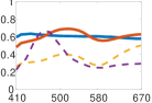
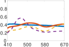
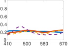
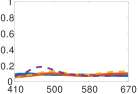
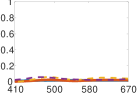
(d) Comparison of the estiamted spectral reflectance results by our method (red line) and two existing single-view methods (yellow line [18] and purple line [5]) using the projector-camera pair 4

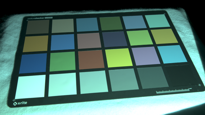
Pair 1	Pair 2
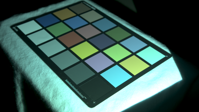
Pair 3	Pair 4

(c) Example captured images

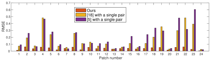
(e) RMSE comparison for each patch of the colorchart

Figure 8: Spectral reflectance estimation results on the 24 patches of the colorchart. As can be seen in (d) and (e), the existing single-view image-based methods [18, 5] fail to correctly estimate the spectral reflectance of each patch (including relative scales between patches) due to the shading effect apparent in the colorchart setup, as shown in (c). In contrast, our method can accurately estimate the spectral reflectance including the relative scales by considering the geometric relationship between the 3D points and the projector positions.

4.3 Spectral reflectance estimation results

To evaluate the performance of our spectral reflectance estimation method, we used a standard colorchart with the 24 patches. We first show the effect of the number of spectral bands. In our experiment, seven color illuminations and RGB camera channels, as shown in Fig. 4, were used, resulting in a total of 21-band measurements. To select the best band set, we evaluated all possible band sets for each number of spectral bands. Figure 7 shows RMSE for the 24 patches of the colorchart when using the selected best band set for each number of spectral bands. We can observe that RMSE is reduced by using multispectral information and becomes very close when more than six bands are used. The six-band set of ($light$, $camera$) = ($L_{green}$, $C_{blue}$), ($L_{blue}$, $C_{green}$), ($L_{blue}$, $C_{blue}$), ($L_{cyan}$, $C_{red}$), ($L_{magenta}$, $C_{red}$), ($L_{yellow}$, $C_{green}$) provides the minimium RMSE among the evaluated all possible band sets.

We next demonstrate the effectiveness of our spectral reflectance estimation model considering the geometric information. As shown in Fig. 8(a), we laid the colorchart on a table and captured the structured light and multispectral data by four projector-camera pairs according to the data acquisition procedure of Pro-Cam SSfM. The estimated projector positions, camera positions, and 3D points of the colorchart are shown in Fig. 8(b). The example captured images (under white illumination) by four projector-camera pairs are shown in Fig. 8(c). Figure 8(d) compares the estimated spectral refletance results for the 24 patches, where the blue line is the ground truth, the red line is our result (average withing each patch) using all projector-camera pairs, and the yellow and purple dashed lines are the results of two existing single-view image-based methods [18, 5] (average withing each patch) only using the projector-camera pair 4. Figure 8(e) shows the corresponding RMSE comparison for each patch, where we can confirm that our method achieves much lower RMSE than the existing methods.

As can be seen in Fig. 8(d) and 8(e), the single-view methods fail to correctly estimate the spectral reflectance including the relative scales between the patches. This is due to the shading effect appeared in the colorchart setup, as shown in Fig. 8(c). In contrast, our method can provide accurate estimation results with correct relative scales. The benefit of our method is to estimate the spectral reflectance while considering the shading effect, which is ignored in the single-view methods. With this essential difference, our method is especially beneficial when the shading exists in the scene. If the shading does not exist, the accuracy of our method could be similar to that of the existing methods. However, such no-shading condition is very special and possible only under fully controlled illumination.

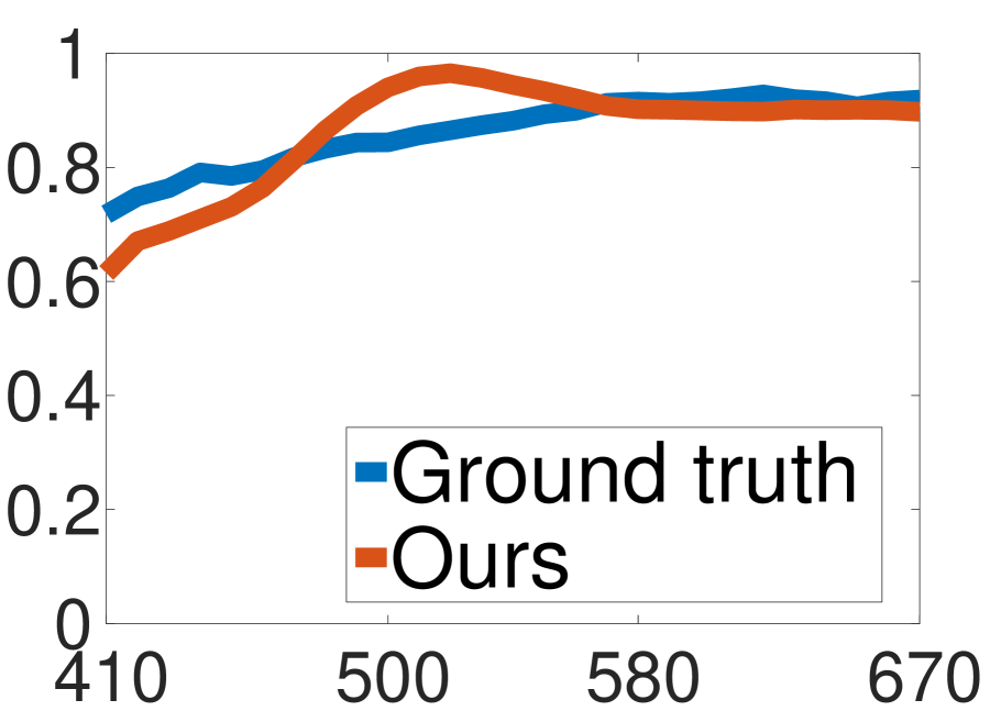
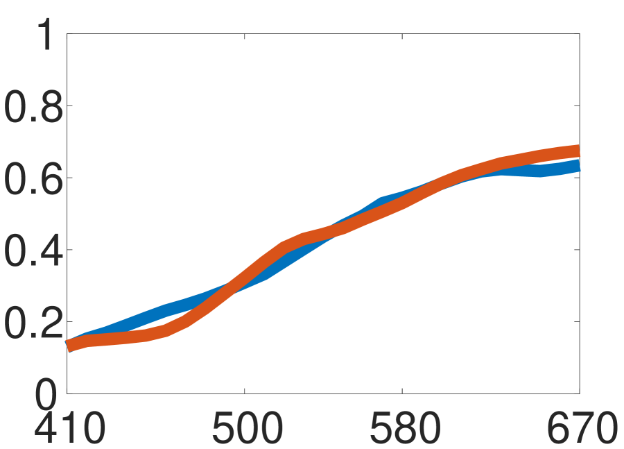
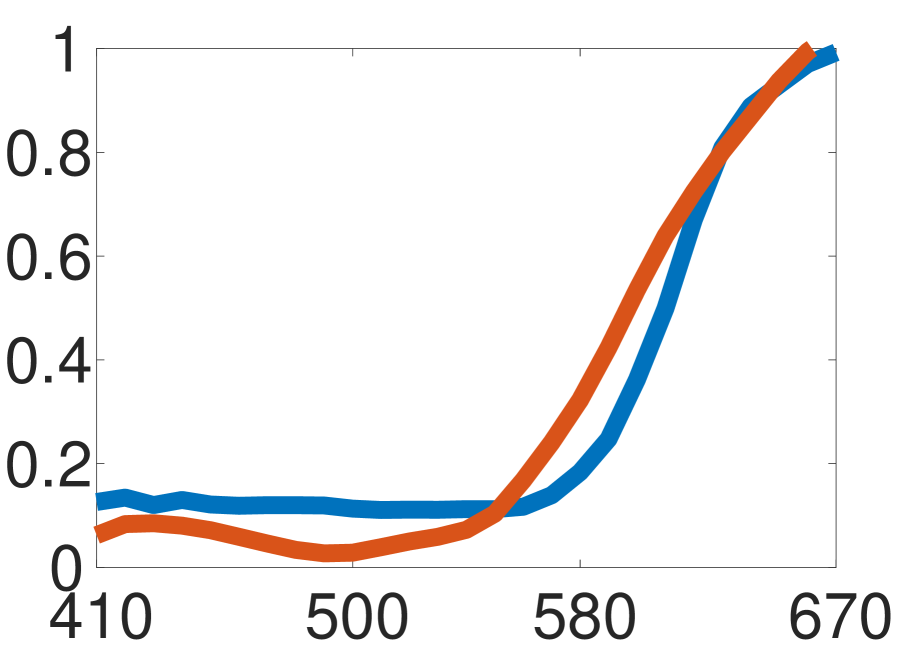
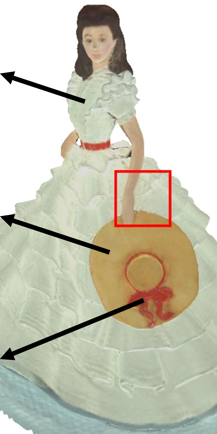
(a) Our result (sRGB)

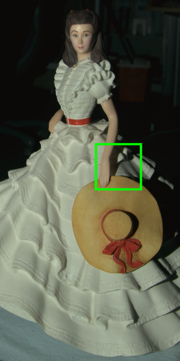
(b) Method [18]

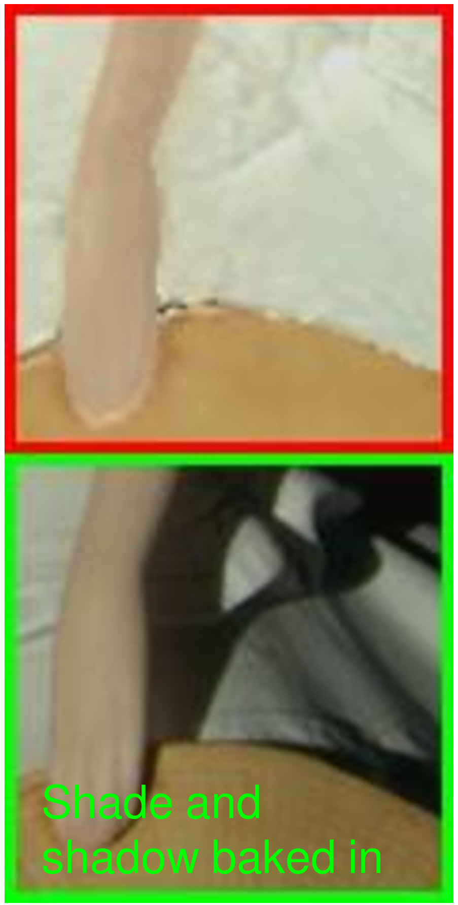
(c) Closeup

\begin{overpic}[scale={.108}]{scarlet_cyan_camera.png} \put(0.0,55.0){\includegraphics[scale={.11}]{cyan.pdf}} \end{overpic}\begin{overpic}[scale={.107}]{groundtruth_cyan.png} \end{overpic}

(d) Our 3D relighting result (left) and the reference actual image (right)

\begin{overpic}[scale={.12}]{doublelight2.png} \put(-3.0,65.0){\includegraphics[scale={.08}]{cyan.pdf}} \put(65.0,65.0){\includegraphics[scale={.08}]{halo.pdf}} \end{overpic}

(e) Relighting under two light sources

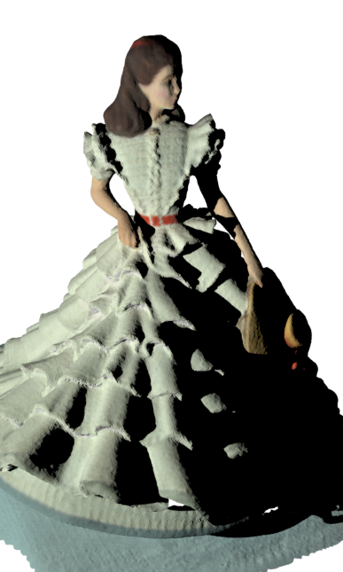
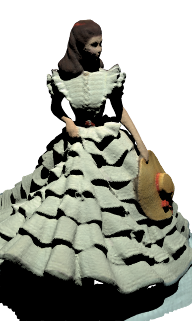
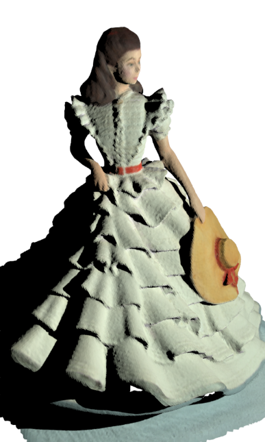
(f) 3D relighting results under different light orientations

Figure 9: Results of the spectral 3D acquisition on a clay sculpture.

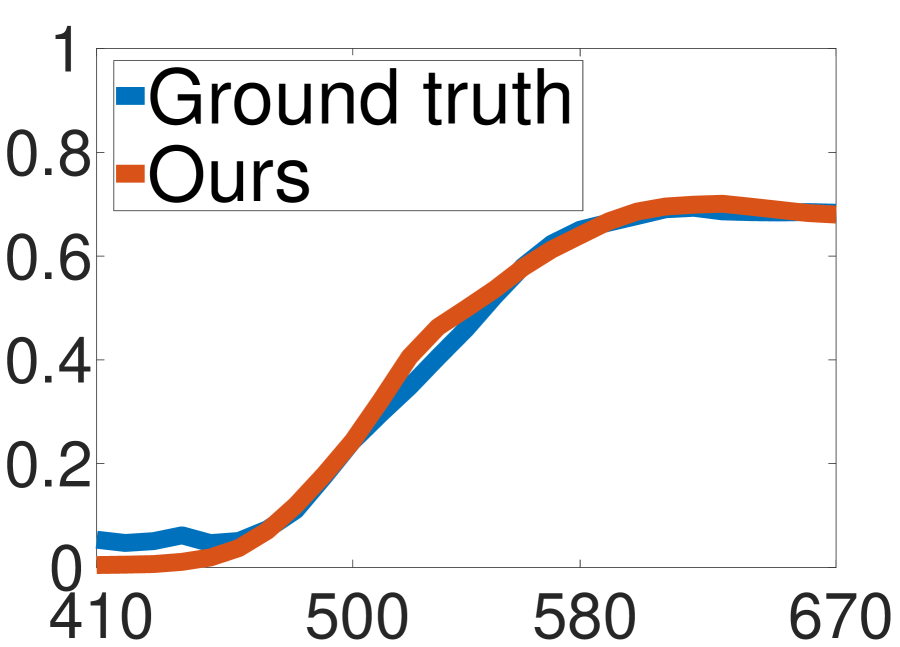
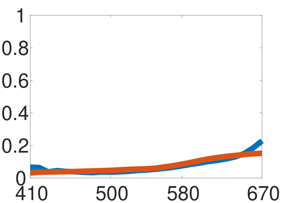
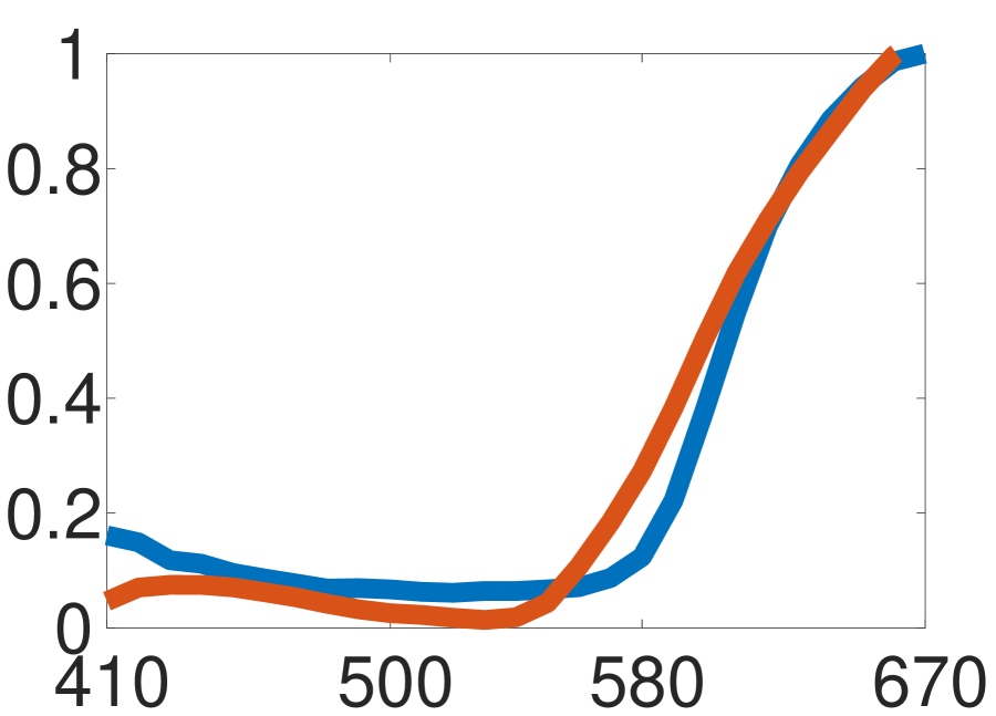
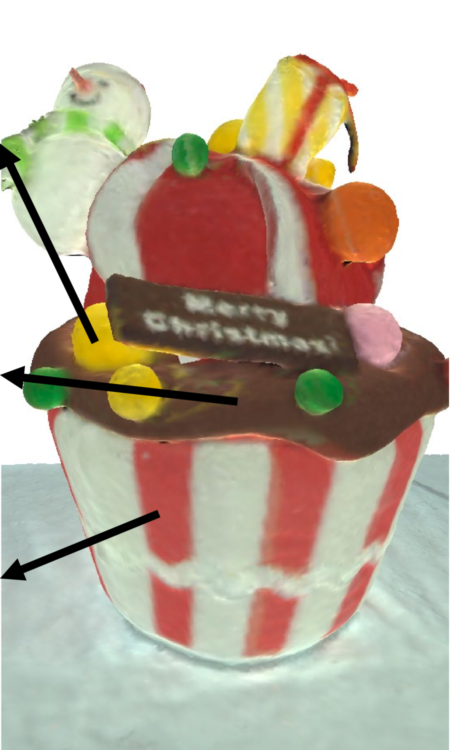
(a) sRGB and reflectance

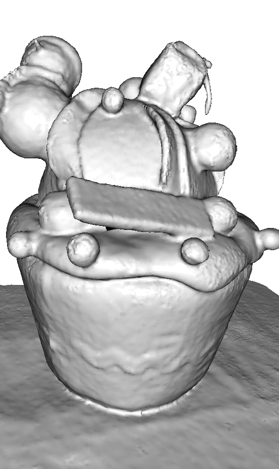
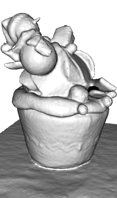
(b) 3D shape

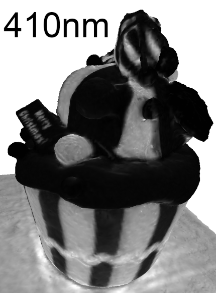
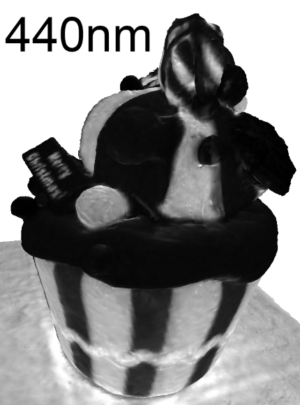
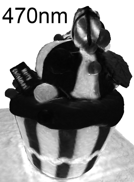
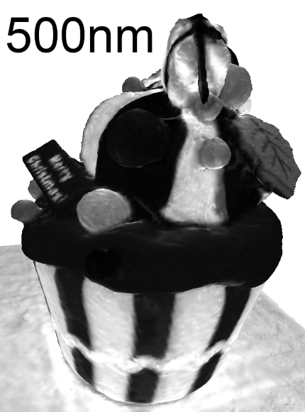
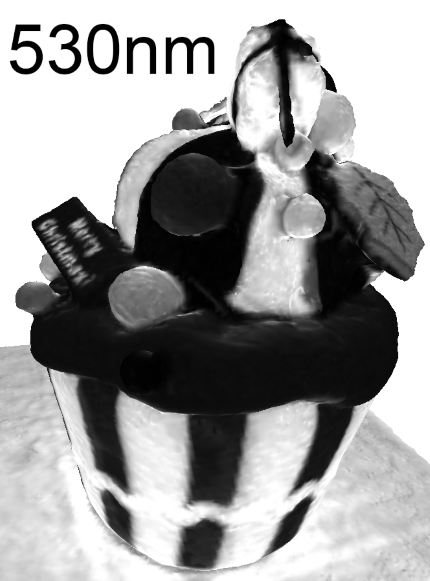
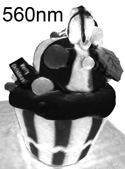
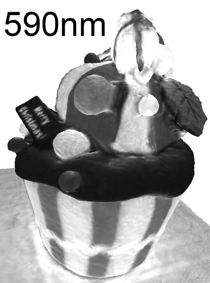
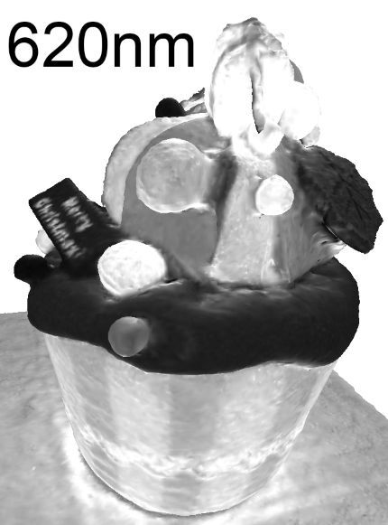
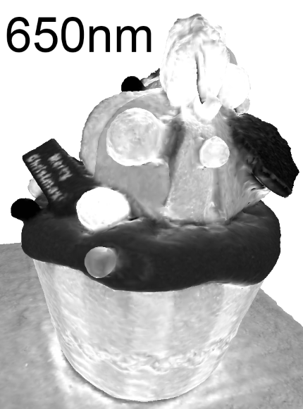
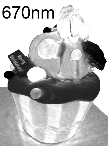
(c) Spectral patterns at each wavelength

Figure 10: Results of the spectral 3D acquisition on a stuffed toy.

4.4 Spectral 3D acquisition results

Figure 9 shows the spectral 3D acquisition result on the clay sculpture. Figure 9(a) shows the spectral reflectance results for some 3D points. It is demonstrated that our method can accurately estimate the spectral reflectance compared with the ground truth measured by a spectrometer. Figure 9(a)–(c) compare the sRGB results converted from the estimated spectral reflectances by our method and the single-view method [18]. We can observe that our spectral reflectance estimation model considering the geometric information can effectively remove the baked-in effect of the shading and the shadow, which is apparent in the sRGB result of the single-view method.

Since Pro-Cam SSfM can accurately estimate both the 3D points and the spectral reflectance, it is possible to perform the spectral 3D relighting of the object for synthesizing the appearance illuminated under an arbitrary light orientation and spectral distribution. Figure 9(d) shows the result of spectral relighting under the projector-cyan illumination, where we can confirm that our relighting result is close to the reference actual image taken in the same illumination orientation and spectral distribution. The differences at the concave skirt regions are due to the effect of interreflections, which is not considered in our current model. Figure 9(e) shows the more complex relighting result under two mixed light sources (projector cyan and halogen lamp), which are located at different sides of the object. Figure 9(f) shows the 3D relighting results under different illumination orientations. As shown in those results, we can effectively perform the spectral 3D relighting based on the estimated 3D model and spectral refletance.

Figure 10 shows the spectral 3D acquisition result on a stuffed toy. Figure 10(a)–(c) respectively show the spectral reflectance and the sRGB results, the 3D shape results, and the spectral patterns at each wavelength. The presented results demonstrate the potential of Pro-Cam SSfM for accurate spectral 3D scanning and rendering. Additional results can be seen in the supplemental video.

5 Concluding Remarks

In this paper, we have proposed Pro-Cam SSfM, the fist spectral 3D acquisition system using an off-the-shelf projector and camera. By effectively exploiting the projector as active lighting for both the geometric and the photometric observations, Pro-Cam SSfM can accurately reconstruct a dense object 3D model with the spectral reflectance property. We have validated that our proposed spectral reflectance estimation model can effectively eliminate the shading effect by incorporating the geometric relationship between the 3D points and the projector positions into the cost optimization. We have experimentally demonstrated the potential of Pro-Cam SSfM through the spectral 3D acquisition results on several real objects.

Pro-Cam SSfM has several limitations. First, we currently assume that the illumination spectrum is known. Second, our spectral reflectance estimation model currently ignores interreflections. Possible future research directions are to address each limitation by simultaneously estimating the spectral reflectance and the illumination spectrum [48] or separating direct and global components by using projected high frequency illumination [37].

Acknowledgment This work was partly supported by JSPS KAKENHI Grant Number 17H00744.

References

- [1] Munsell colors matt. http://cs.joensuu.fi/ spectral/databases/download/munsell_spec_matt.htm.
- [2] Jonas Aeschbacher, Jiqing Wu, and Radu Timofte. In defense of shallow learned spectral reconstruction from RGB images. Proc. of IEEE Int, Conf. on Computer Vision (ICCV) Workshops, pages 471–479, 2017.
- [3] Sameer Agarwal and Keir Mierle. Ceres solver. http://ceres-solver.org.
- [4] Daniel G. Aliaga and Yi Xu. Photogeometric structured light: A self-calibrating and multi-viewpoint framework for accurate 3D modeling. Proc. of IEEE Conf. on Computer Vision and Pattern Recognition (CVPR), pages 1–8, 2008.
- [5] Boaz Arad and Ohad Ben-Shahar. Sparse recovery of hyperspectral signal from natural RGB images. Proc. of European Conf. on Computer Vision (ECCV), pages 19–34, 2016.
- [6] Seung-Hwan Baek, Incheol Kim, Diego Gutierrez, and Min H. Kim. Compact single-shot hyperspectral imaging using a prism. ACM Trans. on Graphics, 36(6):217:1–12, 2017.
- [7] Jan Behmann, Anne-Katrin Mahlein, Stefan Paulus, Jan Dupuis, Heiner Kuhlmann, Erich-Christian Oerke, and Lutz Plümer. Generation and application of hyperspectral 3D plant models: Methods and challenges. Machine Vision and Applications, 27(5):611–624, 2016.
- [8] Xun Cao, Hao Du, Xin Tong, Qionghai Dai, and Stephen Lin. A prism-mask system for multispectral video acquisition. IEEE Trans. on Pattern Analysis and Machine Intelligence, 33(12):2423–2435, 2011.
- [9] Camille Simon Chane, Alamin Mansouri, Franck Marzani, and Frank Boochs. Integration of 3D and multispectral data for cultural heritage applications: Survey and perspectives. Image and Vision Computing, 31(1):91–102, 2013.
- [10] Cui Chi, Hyunjin Yoo, and Moshe Ben-Ezra. Multi-spectral imaging by optimized wide band illumination. Int. Journal of Computer Vision, 86:140–151, 2010.
- [11] Paolo Cignoni, Marco Callieri, Massimiliano Corsini, Matteo Dellepiane, Fabio Ganovelli, and Guido Ranzuglia. Meshlab: An open-source mesh processing tool. Proc. of Eurographics Italian Chapter Conference, pages 129–136, 2008.
- [12] Kate Devlin, Alan Chalmers, Alexander Wilkie, and Werner Purgathofer. Tone reproduction and physically based spectral rendering. Eurographics State of The Art Report, pages 1–23, 2002.
- [13] Ying Fu, Yongrong Zheng, Lin Zhang, and Hua Huang. Spectral reflectance recovery from a single RGB image. IEEE Trans. on Computational Imaging, 4(3):382–394, 2018.
- [14] Ryo Furukawa, Ryusuke Sagawa, Hiroshi Kawasaki, Kazuhiro Sakashita, Yasushi Yagi, and Naoki Asada. One-shot entire shape acquisition method using multiple projectors and cameras. Proc. of Pacific-Rim Symposium on Image and Video Technology (PSIVT), pages 107–114, 2010.
- [15] Yasutaka Furukawa and Jean Ponce. Accurate, dense, and robust multiview stereopsis. IEEE Trans. on Pattern Analysis and Machine Intelligence, 32(8):1362–1376, 2010.
- [16] Sergio Garrido-Jurado, Rafael Muñoz-Salinas, Francisco José Madrid-Cuevas, and Manuel J. Marín-Jiménez. Simultaneous reconstruction and calibration for multi-view structured light scanning. Journal of Visual Communication and Image Representation, 39:120–131, 2016.
- [17] Jason Geng. Structured-light 3D surface imaging: A tutorial. Advances in Optics and Photonics, 3(2):128–160, 2011.
- [18] Shuai Han, Imari Sato, Takahiro Okabe, and Yoichi Sato. Fast spectral reflectance recovery using DLP projector. Int. Journal of Computer Vision, 110(2):172–184, 2014.
- [19] Keita Hirai, Ryosuke Nakahata, and Takahiko Horiuchi. Measuring spectral reflectance and 3D shape using multi-primary image projector. Proc. of Int. Conf. on Image and Signal Processing (ICISP), pages 137–147, 2016.
- [20] Hugues Hoppe, Tony DeRose, Tom Duchamp, John McDonald, and Werner Stuetzle. Surface reconstruction from unorganized points. Proc. of SIGGRAPH, pages 71–78, 1992.
- [21] Shuya Ito, Koichi Ito, Takafumi Aoki, and Masaru Tsuchida. A 3D reconstruction method with color reproduction from multi-band and multi-view images. Proc. of Asian Conf. on Computer Vision (ACCV), pages 236–247, 2016.
- [22] Yan Jia, Yinqiang Zheng, Lin Gu, Art Subpa-Asa, Antony Lam, Yoichi Sato, and Imari Sato. From RGB to spectrum for natural scenes via manifold-based mapping. Proc. of IEEE Int. Conf. on Computer Vision (ICCV), pages 4705–4713, 2017.
- [23] Jun Jiang, Dengyu Liu, Jinwei Gu, and Sabine Süsstrunk. What is the space of spectral sensitivity functions for digital color cameras? Proc. of Workshop on Applications of Computer Vision (WACV), pages 168–179, 2013.
- [24] Michael Kazhdan, Matthew Bolitho, and Hugues Hoppe. Poisson surface reconstruction. Proc. of Eurographics Symposium on Geometry Processing, pages 61–70, 2006.
- [25] Michael Kazhdan and Hugues Hoppe. Screened Poisson surface reconstruction. ACM Trans. on Graphics, 32(3):29:1–13, 2013.
- [26] Kichang Kim, Akihiko Torii, and Masatoshi Okutomi. Multi-view inverse rendering under arbitrary illumination and albedo. Proc. of European Conf. on Computer Vision (ECCV), pages 750–767, 2016.
- [27] Min H. Kim, Todd Alan Harvey, David S. Kittle, Holly Rushmeier, Julie Dorsey, Richard O. Prum, and David J. Brady. 3D imaging spectroscopy for measuring hyperspectral patterns on solid objects. ACM Trans. on Graphics, 31(4):38:1–11, 2012.
- [28] Min H. Kim, Holly Rushmeier, John Ffrench, Irma Passeri, and David Tidmarsh. Hyper3D: 3D graphics software for examining cultural artifacts. ACM Journal on Computing and Cultural Heritage, 7(3):14:1–19, 2014.
- [29] Masahiro Kitahara, Takahiro Okabe, Christian Fuchs, and Hendrik P. A. Lensch. Simultaneous estimation of spectral reflectance and normal from a small number of images. Proc. of Int. Conf. on Computer Vision Theory and Applications (VISAPP), pages 303–313, 2015.
- [30] Chunyu Li, Akihiko Torii, and Masatoshi Okutomi. Robust, precise, and calibration-free shape acquisition with an off-the-shelf camera and projector. Proc. of IEEE Conf. on Consumer Electronics (ICCE), pages 1–6, 2018.
- [31] Jie Liang, Ali Zia, Jun Zhou, and Xavier Sirault. 3D plant modelling via hyperspectral imaging. Proc. of IEEE Int, Conf. on Computer Vision Workshops (ICCVW), pages 172–177, 2013.
- [32] Manolis Lourakis and Antonis A. Argyros. SBA: A software package for generic sparse bundle adjustment. ACM Trans. on Mathematical Software, 36(1):2:1–30, 2009.
- [33] Alamin Mansouri, Alexandra Lathuiliere, Franck Marzani, Yvon Voisin, and Pierre Gouton. Toward a 3D multispectral scanner: An application to multimedia. IEEE Multimedia, 14(1):40–47, 2007.
- [34] Daniel Maurer, Yong Chul Ju, Michael Breuß, and Andrés Bruhn. Combining shape from shading and stereo: A variational approach for the joint estimation of depth, illumination and albedo. Proc. of British Machine Vision Conference (BMVC), pages 76–1–14, 2016.
- [35] Jean Mélou, Yvain Quéau, Jean-Denis Durou, Fabien Castan, and Daniel Cremers. Variational reflectance estimation from multi-view images. Journal of Mathematical Imaging and Vision, 60(9):1527–1546, 2018.
- [36] Yusuke Monno, Sunao Kikuchi, Masayuki Tanaka, and Masatoshi Okutomi. A practical one-shot multispectral imaging system using a single image sensor. IEEE Trans. on Image Processing, 24(10):3048–3059, 2015.
- [37] Shree K. Nayar, Gurunandan Krishnan, Michael D. Grossberg, and Ramesh Raskar. Fast separation of direct and global components of a scene using high frequency illumination. ACM Trans. on Graphics, 25(3):935–944, 2006.
- [38] Rang H. M. Nguyen, Dilip K. Prasad, and Michael S. Brown. Training-based spectral reconstruction from a single RGB image. Proc. of European Conf. on Computer Vision (ECCV), pages 186–201, 2014.
- [39] Keisuke Ozawa, Imari Sato, and Masahiro Yamaguchi. Hyperspectral photometric stereo for a single capture. Journal of the Optical Society of America A, 34(3):384–394, 2018.
- [40] Jong-Il Park, Moon-Hyun Lee, Michael D. Grossberg, and Shree K. Nayar. Multispectral imaging using multiplexed illumination. Proc. of IEEE Int. Conf. on Computer Vision (ICCV), pages 1–8, 2007.
- [41] Jussi P. S. Parkkinen, Jarmo Hallikainen, and Timo Jaaskelainen. Characteristic spectra of Munsell colors. Journal of the Optical Society of America A, 6(2):318–322, 1989.
- [42] Joaquim Salvi, Sergio Fernandez, Tomislav Pribanic, and Xavier Llado. A state of the art in structured light patterns for surface profilometry. Pattern Recognition, 43(8):2666–2680, 2010.
- [43] Johannes L. Schonberger and Jan-Michael Frahm. Structure-from-motion revisited. Proc. of IEEE Conf. on Computer Vision and Pattern Recognition (CVPR), pages 4104–4113, 2016.
- [44] Steven M. Seitz, Brian Curless, James Diebel, Daniel Scharstein, and Richard Szeliski. A comparison and evaluation of multi-view stereo reconstruction algorithms. Proc. of IEEE Conf. on Computer Vision and Pattern Recognition (CVPR), pages 519–528, 2006.
- [45] Zhan Shi, Chang Chen, Zhiwei Xiong, Dong Liu, and Feng Wu. HSCNN+: Advanced CNN-based hyperspectral recovery from RGB images. Proc. of IEEE Conf. on Computer Vision and Pattern Recognition (CVPR) Workshops, pages 939–947, 2018.
- [46] Noah Snavely, Steven M. Seitz, and Richard Szeliski. Photo tourism: Exploring photo collections in 3D. ACM Trans. on Graphics, 25(3):835–846, 2006.
- [47] Michael Weinmann, Christopher Schwartz, Roland Ruiters, and Reinhard Klein. A multi-camera, multi-projector super-resolution framework for structured light. Proc. of Int. Conf. on 3D Imaging, Modeling, Processing, Visualization and Transmission (3DIMPVT), pages 397–404, 2011.
- [48] Seoung Wug Oh, Michael S. Brown, Marc Pollefeys, and Seon Joo Kim. Do it yourself hyperspectral imaging with everyday digital cameras. Proc. of IEEE Conf. on Computer Vision and Pattern Recognition (CVPR), pages 2461–2469, 2016.
- [49] Ali Zia, Jie Liang, Jun Zhou, and Yongsheng Gao. 3D reconstruction from hyperspectral images. Proc. of IEEE Winter Conf. on Applications of Computer Vision (WACV), pages 318–325, 2015.