Turbulence vs. fire hose instabilities: 3-D hybrid expanding box simulations

Abstract

The relationship between a decaying plasma turbulence and proton fire hose instabilities in a slowly expanding plasma is investigated using three-dimensional (3-D) hybrid expanding box simulations. We impose an initial ambient magnetic field along the radial direction, and we start with an isotropic spectrum of large-scale, linearly-polarized, random-phase Alfvénic fluctuations with zero cross-helicity. A turbulent cascade rapidly develops and leads to a weak proton heating that is not sufficient to overcome the expansion-driven perpendicular cooling. The plasma system eventually drives the parallel and oblique fire hose instabilities that generate quasi-monochromatic wave packets that reduce the proton temperature anisotropy. The fire hose wave activity has a low amplitude with wave vectors quasi-parallel/oblique with respect to the ambient magnetic field outside of the region dominated by the turbulent cascade and is discernible in one-dimensional power spectra taken only in the direction quasi-parallel/oblique with respect to the ambient magnetic field; at quasi-perpendicular angles the wave activity is hidden by the turbulent background. These waves are partly reabsorbed by protons and partly couple to and participate in the turbulent cascade. Their presence reduces kurtosis, a measure of intermittency, and the Shannon entropy but increases the Jensen-Shannon complexity of magnetic fluctuations; these changes are weak and anisotropic with respect to the ambient magnetic field and it’s not clear if they can be used to indirectly discern the presence of instability-driven waves.

1 Introduction

The solar wind is a turbulent flow of weakly collisional plasma and constitutes a natural laboratory for plasma turbulence (Bruno & Carbone, 2013; Alexandrova et al., 2013). Properties of plasma turbulence and its dynamics remain an open challenging problem (Petrosyan et al., 2010; Matthaeus & Velli, 2011). At large scales it can be described by the magnetohydrodynamic (MHD) approximation, accounting for the dominant nonlinear coupling and for the presence of the ambient magnetic field that introduces a preferred direction (Shebalin et al., 1983; Oughton et al., 1994; Verdini et al., 2015). Around particle characteristic scales the plasma description has to be extended beyond MHD (cf., Papini et al., 2019, and references therein) and a transfer of the cascading energy to particles is expected. Observed radial profiles of proton temperatures indicate an important heating which is often comparable to the estimated turbulent energy cascade rate (MacBride et al., 2008; Cranmer et al., 2009; Hellinger et al., 2013). Alpha particles also need to be heated (Stansby et al., 2019) whereas for electrons it is much less clear because of their strong heat flux (Štverák et al., 2015).

The nonlinearly coupled turbulent system is also characterized by non-Gaussian statistical properties, a phenomenon called intermittency. For a given quantity $Y$ (e.g., a component of the magnetic field, bulk velocity field) and a separation length $l$, the increment, $\Delta Y$, the difference between two points separated by $l$, has generally a non-Gaussian distribution. This non-Gaussianity is well characterized by the excess kurtosis (flatness) that is close to zero on large scales (compatible with a Gaussian statistics) but it increases as $l$ decreases in the inertial ranges; behavior of the kurtosis in the sub-ion range is not well known, some results indicate that it further increases (e.g., Alexandrova et al., 2008; Franci et al., 2015) but some observations and numerical simulations indicate that the kurtosis saturates and even decreases in the sub-ion range (e.g., Wu et al., 2013; Parashar et al., 2018). The non-Gaussian statistics with extreme values is often associated with localized/coherent structures that appear to be important for the particle energization (Matthaeus et al., 2015); these energization/dissipation processes could be responsible for the decrease of the kurtosis.

Recently, the Shannon entropy, $H$, and the Jensen-Shannon complexity, $C$ (see below for definitions), two related quantities that measure the information content in time series and allows to discern chaotic versus stochastic behavior (Maggs & Morales, 2013), were used to characterize also turbulent fluctuations observed in situ or in laboratory plasmas (Weck et al., 2015). The time series of the solar wind magnetic field exhibit a relatively large normalized permutation (Shannon) entropy ($H\gtrsim 0.9$), and a small statistical (Jensen-Shannon) complexity ($C\lesssim 0.15$) (Weck et al., 2015; Weygand & Kivelson, 2019; Olivier et al., 2019). In situ observations also indicate that during the radial evolution the permutation entropy $H$ increases whereas the complexity $C$ decreases and these statistical parameters in the ($H,C$) plane have properties similar to those predicted for a fractional Brownian motion (Weygand & Kivelson, 2019); interestingly, the fractional Brownian motion may be regarded as a natural boundary between chaotic and stochastic processes (Maggs & Morales, 2013); however, the connection between these two statistical parameters and properties of the solar wind turbulence is yet unclear.

The radial expansion further complicates the evolution of the solar wind turbulence. It induces an additional damping, turbulent fluctuations decrease due to the expansion (as well as due to the turbulent decay) slowing down the turbulent cascade (cf., Grappin et al., 1993; Dong et al., 2014). Furthermore, the expansion also introduces another preferred direction (the radial one) (Verdini & Grappin, 2015) and the characteristic particle scales change with the radial distance. The understanding of the complex nonlinear properties of plasma turbulence on particle scales is facilitated via a numerical approach (Servidio et al., 2015; Franci et al., 2018b). Direct kinetic simulations of turbulence show that particles are indeed on average heated by the cascade (Parashar et al., 2009; Markovskii & Vasquez, 2011; Wu et al., 2013; Franci et al., 2015; Arzamasskiy et al., 2019), and, moreover, turbulence leads locally to complex anisotropic and nongyrotropic distribution functions (Valentini et al., 2014; Servidio et al., 2015). On the other hand, the solar wind expansion naturally generates particle temperature anisotropies (Matteini et al., 2007, 2012). The anisotropic and nongyrotropic features may be a source of free energy for kinetic instabilities. There are indications that such instabilities are active in the solar wind. Apparent bounds on ion parameters are observed that are relatively in agreement with theoretical kinetic linear predictions (Gary et al., 2001; Hellinger et al., 2006; Maruca et al., 2012; Matteini et al., 2013; Klein et al., 2018). Furthermore, wave activity driven by the kinetic instabilities associated with the ion temperature anisotropies and/or differential velocity is often observed (Jian et al., 2009; Gary et al., 2016; Wicks et al., 2016). This activity is usually in the form of a narrow-band enhancement of the magnetic power spectral density at ion scales ‘on top of’ the background turbulent magnetic field; these fluctuations tend to be relatively coherent (Lion et al., 2016).

Hellinger et al. (2015) used a two-dimensional (2-D) hybrid expanding box (HEB) model to study the relationship between the proton oblique fire hose instability and plasma turbulence. They showed that the instability and plasma turbulence can coexist and that the instability bounds the proton temperature anisotropy in an inhomogeneous/nonuniform turbulent system. The results of Hellinger et al. (2015) are, however, strongly constrained by the 2-D geometry with the ambient magnetic field being perpendicular to the simulation plane and one expects that unstable modes appear at quasi-parallel/oblique angles with respect to the background magnetic field based on the linear (uniform and homogeneous) theory (cf., Gary, 1993; Klein & Howes, 2015). In this paper we extend the work of Hellinger et al. (2015) using a 3-D version of the HEB model. We investigate the real-space and spectral properties of turbulent fluctuations and the impact of fire hose driven waves. We also analyze the effects of this wave activity on the statistical properties (intermittency, permutation entropy, complexity) of turbulence and test if these quantities could be used as a mean to discern the presence of the fire hose waves.

2 Numerical Code

In this paper we use a 3-D version of the HEB model implemented in the numerical code CAMELIA (Franci et al., 2018a) that allows us to study self-consistently different physical processes at ion scales (cf., Ofman, 2019). The expanding box uses coordinates co-moving with the solar wind plasma, assuming a constant solar wind radial velocity $v_{sw}$, and approximating the spherical coordinates by the Cartesian ones (Hellinger & Trávníček, 2005). The radial distance $R$ of the box follows $R=R_{0}(1+t/t_{\text{exp}})$ where $R_{0}$ is the initial position and $t_{\text{exp}}=R_{0}/v_{sw}$ is the (initial) characteristic expansion time. Transverse scales of the simulation box (with respect to the radial direction) increase $\propto R$ whereas the radial scale remains constant. The model uses the hybrid approximation where electrons are considered as a massless, charge neutralizing fluid and ions are described by a particle-in-cell model (Matthews, 1994). Fields and moments are defined on a 3-D grid $512\times 512\times 256$; periodic boundary conditions are assumed. The initial spatial resolution is $\Delta x=\Delta y=0.25d_{i}$, $\Delta z=0.5d_{i}$ where $d_{i}=v_{A}/\omega_{ci}$ is the initial proton inertial length ($v_{A}$: the initial Alfvén velocity, $\omega_{ci}$: the initial proton gyrofrequency). There are $400$ macroparticles per cell for protons which are advanced with a time step $\Delta t=0.05/\omega_{ci}$ while the magnetic field is advanced with a smaller time step $\Delta t_{B}=\Delta t/10$. The initial ambient magnetic field is directed along the $z$ (radial) direction, $\bm{B}_{0}=(0,0,B_{0})$, and we impose a continuous expansion in $x$ and $y$ directions with the initial expansion time $t_{\text{exp}}=10^{4}\omega_{ci}^{-1}$. Due to the expansion with the strictly radial magnetic field the ambient density and the magnitude of the ambient magnetic field decrease as $\langle n\rangle\propto\langle B\rangle\propto R^{-2}$ (the proton inertial length $d_{i}$ increases $\propto R$, the ratio between the transverse sizes and $d_{i}$ remains constant whereas the ratio between the radial size and $d_{i}$ decreases as $R^{-1}$).

We set initially the parallel proton beta $\beta_{\|}=2.4$ and the proton temperature anisotropy $T_{\perp}/T_{\|}=0.75$; for these parameters the plasma system is stable with respect to the fire hose instabilities. Electrons are assumed to be isotropic and isothermal with $\beta_{e}=1$. We initialize the simulation with an isotropic 3-D spectrum of modes with random phases, linear Alfvén polarization ($\delta\bm{B}\perp\bm{B}_{0}$), and vanishing correlation between magnetic and velocity fluctuations (zero cross-helicity). These modes are in the range $0.02\leq kd_{i}\leq 0.2$ and have a flat one-dimensional (1-D) (omnidirectional) power spectrum with rms fluctuations $=0.24B_{0}$. A small resistivity $\eta$ is used to avoid accumulation of cascading energy at grid scales; we set $\eta=0.001\mu_{0}v_{A}^{2}/\omega_{ci}$ ($\mu_{0}$ being the magnetic permittivity of vacuum).

3 Simulation results

3.1 Global evolution

The evolution of the system is shown in Fig. 1 that displays quantities averated over the simulation box: the (rms) total fluctuating magnetic field $\delta B$ and the fluctuating magnetic field $\delta B_{l}$ with large parallel wave vectors (i.e., for for $|k_{\|}|d_{i}>0.25$), the mean square of the electric current, $|\bm{J}|^{2}$, the mean proton temperature anisotropy $T_{\perp}/T_{\|}$, and the mean proton agyrotropy $A_{\diameter}$ as functions of time. The agyrotropy $A_{\diameter}$ is defined here following Scudder & Daughton (2008) as

$$A_{\diameter}=2\frac{|P_{\perp 1}-P_{\perp 2}|}{P_{\perp 1}+P_{\perp 2}}$$ (1)

where $P_{\perp 1}$ and $P_{\perp 2}$ are the are the two eigenvalue components of the (proton) pressure tensor perpendicular to the local magnetic field.

The level of total magnetic fluctuations, $\delta B$ initially shortly increases as the turbulent cascade develops and a part of the kinetic proton energy is transformed to the magnetic one (cf., Franci et al., 2015). After that short transient period, $\delta B$ overall decreases and oscillates with a small amplitude due to superposition of large-scale propagating Alfvén modes. The amplitude of magnetic fluctuations with $|k_{\|}|d_{i}>0.25$, $\delta B_{l}$, (top panel of Fig. 1, dashed line) initially increases, reaches a local maximum around $t=0.025t_{\text{exp}}$ as the turbulent cascade develops. After that it decreases until it reaches another local maximum at about $t=0.13t_{\text{exp}}$. The mean amplitude of the current, $|\bm{J}|$, initially increases and reaches a maximum at about $t=0.04t_{\text{exp}}$ which indicates the presence of a well-developed turbulent cascade (Mininni & Pouquet, 2009; Valentini et al., 2014). After that, $|\bm{J}|$ decreases with a hint of a slower decrease rate around $t=0.13t_{\text{exp}}$.

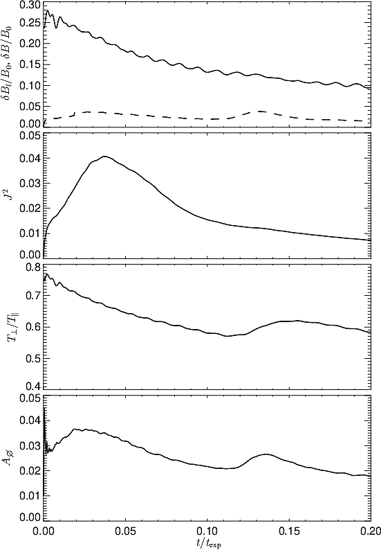
Figure 1: Evolution of (from top to bottom) the total fluctuating magnetic field, $\delta B$ (solid line), and the fluctuating magnetic field with large parallel wave vectors, $\delta B_{l}$ (dashed line), the mean square of the electric current $|\bm{J}|^{2}$, the mean proton temperature anisotropy $T_{\perp}/T_{\|}$, and the mean proton agyrotropy $A_{\diameter}$ as functions of time.

The temperature anisotropy, $T_{\perp}/T_{\|}$, after an initial transition decreases (with weak oscillations) but it increases from $t\sim 0.12t_{\text{exp}}$ to $\sim 0.15t_{\text{exp}}$ (and the system becomes less anisotropic), when modes with large parallel wave vectors appear; after $t\sim 0.16t_{\text{exp}}$, $T_{\perp}/T_{\|}$ decreases again. The agyrotropy, $A_{\diameter}$, starts from the initial noise level $0.01$, strongly varies during the short relaxation of the initial conditions and then increases, reaches a maximum at around $t=0.02t_{\text{exp}}$ and decreases. Later on, at the same time as the proton anisotropy is reduced, the agyrotropy increases again, reaches a maximum around $0.14t_{\text{exp}}$ then and decreases. The turbulent cascade creates velocity shears at ion scales that naturally generate anisotropy as well as agyrotropy (Del Sarto & Pegoraro, 2018). Figure 1 suggests that the reduction of the temperature anisotropy occurring at $t\sim 0.12t_{\text{exp}}$ – $0.15t_{\text{exp}}$ is related to the development of fire hose-like instabilities generating fluctuations with large parallel wave vectors. While the fire hose instabilities driven fluctuations reduce their source of free energy, they enhance the agyrotropy.

Figure 2 shows the evolution of the system in the $(\beta_{\|},T_{\perp}/T_{\|})$ space that is useful to parametrize the linear stability of a (uniform and homogeneous) plasma with respect to temperature anisotropy-driven instabilities (Gary et al., 2001). Figure 2 shows that after the initial transient evolution, $T_{\perp}/T_{\|}$ decreases and $\beta_{\|}$ increases somewhat similarly to the double-adiabatic prediction ($T_{\perp}\propto R^{-2}$, $T_{\|}=\mathrm{const}$.). During this phase, $\beta_{\|}$ increases whereas $T_{\perp}/T_{\|}$ decreases. Eventually, the system reaches parameters that are unstable (with respect to the parallel fire hose) in the corresponding uniform and homogeneous plasma. Before reaching the region unstable with respect to the oblique fire hose instability the system moves towards the stable region and $T_{\perp}/T_{\|}$ increases whereas $\beta_{\|}$ decreases. This reduction of the proton anisotropy stops after some time and $T_{\perp}/T_{\|}$ decreases and $\beta_{\|}$ increases until the end of the simulation. The last part of the path of the system in the $(\beta_{\|},T_{\perp}/T_{\|})$ space is very similar to results from HEB simulations without turbulent fluctuations (cf., Hellinger, 2017) when the system is under the influence of the parallel and oblique fire hose instabilities. The latter is particularly efficient in reducing the proton temperature anisotropy due to its peculiar nonlinear evolution: the oblique fire hose generates non propagating modes that only exist for a sufficiently strong proton parallel temperature anisotropy. As these modes grow they scatter protons and reduce their temperature anisotropy. Consequently, they destroy the non propagating branch and transform (via the linear mode conversion) to propagating modes that are damped and during this process they further reduce the temperature anisotropy (Hellinger & Matsumoto, 2000, 2001). We observe a similar evolution in the present simulation.

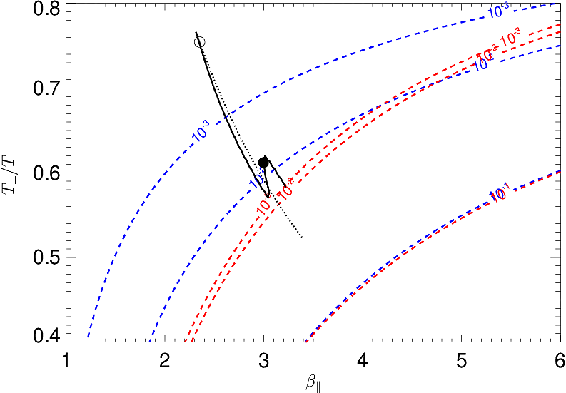
Figure 2: Evolution of the system in the $(\beta_{\|},T_{\perp}/T_{\|})$ space (solid line). The empty circle denotes the initial condition whereas the full circle denotes the time $t=0.14t_{\text{exp}}$; the dotted line shows the double adiabatic prediction for a corresponding system without turbulent fluctuations. Blue and red dashed contours show the maximum growth rate (normalized to $\omega_{ci}$) of the parallel and oblique fire hose instability (for a uniform and homogeneous bi-Maxwellian system), respectively.

3.2 Physical space

We will now look at the properties of the simulated system at three different times, at $t=0.10t_{\text{exp}}$, before the onset of the fire hose instabilities, at $t=0.14t_{\text{exp}}$ around the maximum activity of the instabilities, and at the end, $t=0.20t_{\text{exp}}$. Figure 3 shows the real space structure of the magnetic fluctuations at the three times. It shows 2-D cuts of $\delta B$ as functions of $(x,y)$ and $(z,y)$. At $t=0.10t_{\text{exp}}$ Figure 3 (top panels) show a developed turbulence with complex anisotropic properties. In the $(x,y)$ cut there are signatures of nonlinear structures (such as current sheets and magnetic islands) whereas the $(z,y)$ cut exhibits also large scale wavy behavior (cf., Franci et al., 2018b). At $t=0.14t_{\text{exp}}$ (Figure 3, middle panels) the $(x,y)$ cut remains qualitatively the same as at $t=0.10t_{\text{exp}}$ but in the $(z,y)$ cut there is a clear wave activity, in the form of localized quasi-coherent wave packets (with wavelengths of the order of $10d_{i}$), on top of the turbulent background. At the end, $t=0.20t_{\text{exp}}$, the $(x,y)$ cut is still qualitatively unchanged and the $(z,y)$ cut is similar to that at $t=0.10t_{\text{exp}}$. Note that a similar real space structure is also observed for other quantities (e.g., ion bulk velocity, density, currents, temperature anisotropy/agyrotropy); all these quantities are more uniform along the ambient magnetic field or rather along the magnetic field lines.

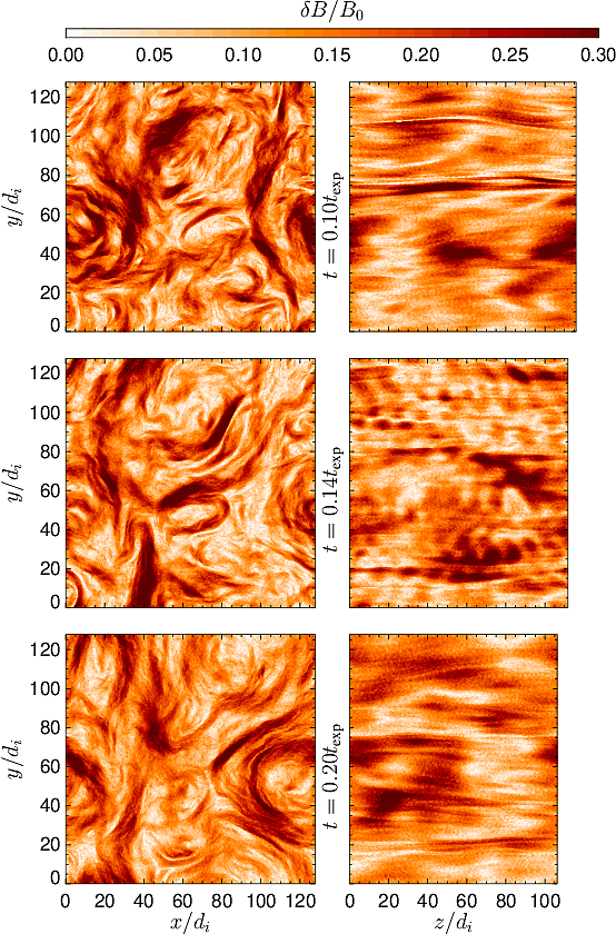
Figure 3: Color scale plots of 2-D cuts of $\delta B$ (normalized to $B_{0}$) as functions of $(x,y)$ (left) and $(z,y)$ (right) for $t=0.10t_{\text{exp}}$ (top), $t=0.14t_{\text{exp}}$ (middle), and $t=0.20t_{\text{exp}}$ (bottom).

To approach in situ 1-D observations we investigate 1-D spatial cuts through the simulation box for the three times. Figure 4 shows 1-D plots of the fluctuating magnetic field components $B_{x}$, $B_{y}$, and $\delta B_{z}$ normalized to $B_{0}$ as functions of $x$ (and $y=z=0$, left) and $z$ (and $x=y=0$, right). As in Figure 3 the perpendicular cuts (Figure 4, left panels) are strongly stuctured but it is hard to discern any similarities between the three times (except perhaps qualitative ones). In the parallel cuts there are mostly large scale fluctuations at $t=0.10t_{\text{exp}}$ and $t=0.20t_{\text{exp}}$. At $t=0.14t_{\text{exp}}$ there are, on top of the large-scale turbulent fluctuations, shorter-wavelength wave packets owing to the fire hose instabilities. Figure 4 also shows that the compressible component $\delta B_{z}$ is weak with respect to $B_{x}$ and $B_{y}$ for the turbulent as well as fire hose fluctuations. Note that the radial ($z$) size of the simulation box normalized to the proton inertial length decreases with time.

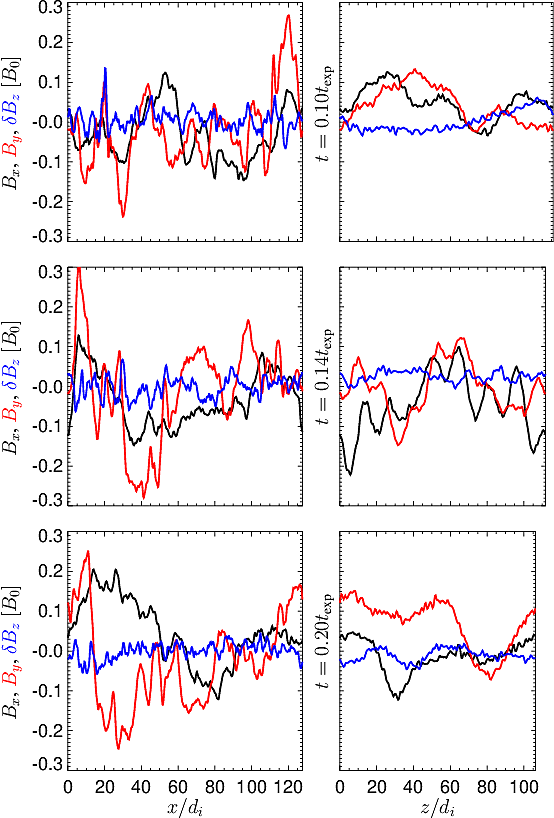
Figure 4: 1-D cuts of the fluctuating magnetic field components (black) $B_{x}$, (red) $B_{y}$, and (blue) $\delta B_{z}$ (normalized to $B_{0}$) as functions of $x$ (and $y=z=0$, left) and $z$ (and $x=y=0$, right) for $t=0.10t_{\text{exp}}$ (top), $t=0.14t_{\text{exp}}$ (middle), and $t=0.20t_{\text{exp}}$ (bottom).

3.3 Spectral properties

Let us now investigate the spectral properties of the fluctuations shown in Fig. 3. Figure 5 shows the 2-D power spectral densities (PSDs) of the magnetic field, $\bm{B}$, and the ion bulk velocity, $\bm{u}$, as functions of $k_{\perp}$ and $k_{\|}$ at the three times. At $t=0.10t_{\text{exp}}$ Figure 5 (top panels) demonstrates that the initial isotropic spectrum develops into a strongly anisotropic one with a cascade preferably at strongly oblique angles with respect to the ambient magnetic field (cf., Franci et al., 2018b). At $t=0.14t_{\text{exp}}$ (Figure 5, middle panels) there is a similar turbulent spectrum and, moreover, a narrow band in $k_{\|}$ (at $k_{\|}\sim 0.5/d_{i}$) enhancement at quasi-parallel/oblique angles with respect to the background magnetic field. At $t=0.20t_{\text{exp}}$ this narrow band enhancement is not clearly discernible but there are some indications that some of the fluctuating energy remained (around $k_{\perp}\sim 0.1/d_{i}$ and $k_{\|}\sim 0.2/d_{i}$).

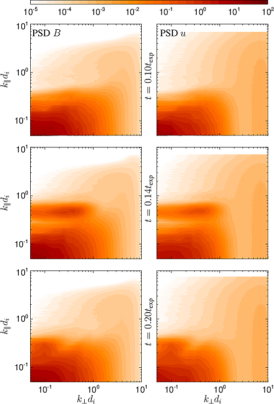
Figure 5: Color scale plots of the power spectral densities of the magnetic field $\bm{B}$ (left) and the proton bulk velocity field $\bm{u}$ (right) as functions of $k_{\perp}$ and $k_{\|}$ for $t=0.10t_{\text{exp}}$ (top), $t=0.14t_{\text{exp}}$ (middle), and $t=0.20t_{\text{exp}}$ (bottom).

It is interesting to look at the reduced 1-D power spectra since these correspond to what is usually obtained from observational spacecraft data. Figure 6 shows the comparison between the reduced parallel and perpendicular 1D power spectral densities of $\bm{B}$ and $\bm{u}$ at the same three times as in Fig. 3. In the perpendicular direction, the PSDs of $\bm{B}$ and $\bm{u}$ as functions of $k_{\perp}$ (Figure 6, left panels) show a little variation between the three times. The fire hose wave activity is not discernible here. The PSDs of $B$ and $u$ exhibit a steepening at ion scales and some noise at smaller scales (numerical noise is especially visible in the velocity fluctuations due to the limited number of particles per cell). On the other hand, in the parallel direction, the PSDs of $\bm{B}$ and $\bm{u}$ as functions of $k_{\|}$ (Figure 6, right panels) exhibit a clear narrow peak at $t=0.14t_{\text{exp}}$ (dashed line) compared to both $t=0.10t_{\text{exp}}$ and $t=0.20t_{\text{exp}}$. Also here the small scale fluctuations are dominated by numerical noise.

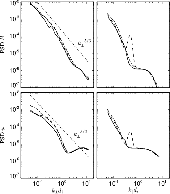
Figure 6: Reduced 1D power spectral densities of (top) $\bm{B}$ and (bottom) $\bm{u}$ as functions of (left) $k_{\perp}$ and (right) $k_{\|}$ for (dash-dotted) $t=0.10t_{\text{exp}}$, (dashed) $t=0.14t_{\text{exp}}$, and (solid) $t=0.20t_{\text{exp}}$. The dotted lines show (top left) a Kolmogorov-like spectrum $\propto k_{\perp}^{-5/3}$ and (bottom left) a spectrum $\propto k_{\perp}^{-3/2}$.

Further analysis shows that only for angles between the ambient magnetic field and the wave vector below $\sim 40^{\mathrm{o}}$ the fire hose fluctuations are discernible in the corresponding reduced 1-D power spectra.

Figure 7 shows the reduced parallel and perpendicular 2-D spatio-temporal spectra of magnetic fluctuations during two phases, $t=0\div 0.1t_{\text{exp}}$ and $t=0.1\div 0.2t_{\text{exp}}$. During the first, turbulent-only phase, the perpendicular spectrum $\delta B(k_{\perp},\omega)$ is broadly distributed around the zero frequency; the spread is very large for $k_{\perp}$ close to $0$. During the second, fire-hose phase the perpendicular spectrum is similar but somewhat weaker. The behaviour of the parallel spectrum $\delta B(k_{\|},\omega)$ is different. During the first phase the spectrum (for small $k_{\|}$) clearly exhibit Alfvénic dispersion, $\omega=\pm k_{\|}\bar{v}_{A}$ (shown by the dotted lines) where $\bar{v}_{A}$ is the mean (over the given time interval) Alfvén velocity including the effects of the proton temperature anisotropy. During the second phase, these Alfvénic fluctuations are reduced and the parallel spectrum further contains fast-magnetosonic dispersive modes ($\omega\propto\pm k_{\|}^{2}$) for $0.2\lesssim k_{\|}\lesssim 0.4$ and weakly or non propagating modes at $0.3\lesssim k_{\|}\lesssim 0.6$. The former modes are likely due to the parallel fire hose (Gary et al., 1998; Matteini et al., 2006) whereas the latter are likely related to the oblique fire hose (Hellinger & Trávníček, 2008).

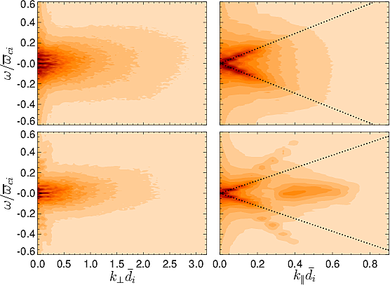
Figure 7: Spatio-temporal spectral properties of magnetic fluctuations: reduced 2-D spectra of $\bm{B}$ as functions of (left) $k_{\perp}$ and $\omega$ and (right) $k_{\|}$ and $\omega$ for (top) $t=0\div 0.1t_{\text{exp}}$ and (bottom) $t=0.1\div 0.2t_{\text{exp}}$. The wavevectors are normalized to the mean (over the given time interval) inertial length $\bar{d}_{i}$ and the frequency is normalized to the mean cyclotron frequency $\overline{\omega}_{ci}$. The dotted lines denote the dispersion relation of Alfvén waves.

3.4 Velocity distribution function

The analysis above indicates that the expansion drives the system unstable with respect to the parallel and oblique fire hose instabilities despite the presence of a developed anisotropic turbulent cascade. The fire hose wave activity appears at quasi-parallel/oblique angles with respect to the background magnetic field, outside the region in $(k_{\perp},k_{\|})$ where the turbulent fluctuations dominate. The generated wave activity is likely partly damped (as expected for the oblique fire hose) and partly blends into the turbulent fluctuations. Figure 8 shows the gyro-averaged proton velocity distribution function at the different times. This figure shows that at $t=0.10t_{e}$ is deformed with respect to the initial bi-Maxwellian distribution function due to the turbulent heating (cf., Arzamasskiy et al., 2019); at $v_{\|}\sim 3v_{A}$ there are signatures of the cyclotron heating owing to the Alfvén (cyclotron) waves. At $t=0.14t_{e}$ the proton velocity distribution function exhibits strong wings due to the standard and anomalous cyclotron resonance between the protons and fire hose waves. The signature of this interaction is weakened at $t=0.20t_{e}$ but still discernible.

Figure 8: Gyro-averaged proton velocity distribution function $f$ as a function of parallel and perpendicular velocities $v_{\|}$ and $v_{\perp}$ (with respect to the background magnetic field) for (top) $t=0.10t_{e}$, (middle) $t=0.14t_{e}$, and (bottom) $t=0.20t_{e}$.

3.5 Statistical properties

It is interesting to look at how the fire hose wave activity affects the statistical properties of turbulence. The turbulent cascade leads to a non-Gaussian character of the fluctuations, i.e., intermittency, which is likely affected by the wave activity generated by the fire hose instabilities. We calculated the excess kurtosis $K^{\prime}=K-3$ in the separation space $(l_{\perp},l_{\|})$ over the simulation box for the increment $\delta B_{y}=B_{y}(x+l_{\perp},y,z+l_{\|})-B_{y}(x,y,z)$. The maximum value of $K^{\prime}$ appears at $l_{\|}=0$ and evolves with the time: initially reaches values of the order of 10 and after $t\simeq 0.05t_{\text{exp}}$ it stays about 3 and slowly decreases; there is no discernible effect of the fire hose instabilities on it. $K^{\prime}$ is, however, very anisotropic. Figure 9 shows $K^{\prime}$ as a function of $l_{\perp}$ and $l_{\|}$ at the three times $t=0.10t_{\text{exp}}$ $t=0.14t_{\text{exp}}$, and $t=0.20t_{\text{exp}}$. The kurtosis is similar at $t=0.10t_{\text{exp}}$ and $t=0.20t_{\text{exp}}$ (at the latter time is somewhat weaker): it’s strongly dependent on $l_{\perp}$, increases as $l_{\perp}$ decreases but when approaching the spatial resolutions $K^{\prime}$ saturates and decreases. At $t=0.14t_{\text{exp}}$ the kurtosis is noticeably reduced at the quasi-parallel direction, likely owing to the presence of quasi-parallel/oblique waves.

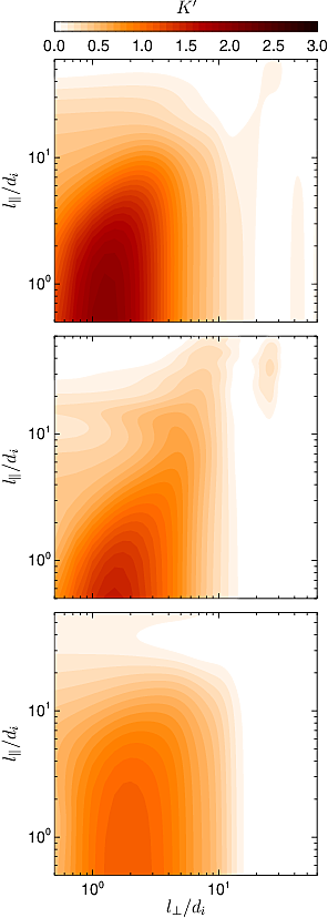
Figure 9: Color scale plots of the excess kurtosis $K^{\prime}$ of the increment $\delta B_{y}$ as functions of the separation $l_{\perp}$ and $l_{\|}$ for (top) $t=0.10t_{\text{exp}}$, (middle) $t=0.14t_{\text{exp}}$, and (bottom) $t=0.20t_{\text{exp}}$.

Finally, it’s interesting to look at how the fire hose wave activity affects the permutation entropy $H$ and the Jensen-Shannon complexity $C$ (López-Ruiz et al., 1995; Bandt & Pompe, 2002; Lamberti et al., 2004). The (normalized) permutation entropy is defined for a time series where for $n$ consecutive points one calculates the probability for each permutation of larger/smaller ordering $p_{j}$. For this probability vector $\bm{p}=\{p_{j}\}_{j=1,n!}$ the information/Shannon entropy is given as

$$S(\bm{p})=-\sum_{p_{j}\neq 0}p_{j}\ln p_{j}$$ (2)

and the permutation entropy $H$ is normalized to its maximum value as

$$H(\bm{p})=\frac{S(\bm{p})}{\ln n!}.$$ (3)

The Jensen-Shannon complexity is given by

$$C(\bm{p})=Q(\bm{p})H(\bm{p})$$ (4)

where

$$Q(\bm{p})=-\frac{2S(\frac{\bm{p}+\bm{p}_{e}}{2})-S(\bm{p})-S(\bm{p}_{e})}{\frac{n!+1}{n!}\ln(n!+1)-2\ln(2n!)+\ln n!}$$ (5)

is a measure of the distance between $\bm{p}$ and $\bm{p}_{e}$, the probability vector for equally probable permutations, $\bm{p}_{e}=\{1/n!\}_{j=1,n!}$.

The two statistical quantities depend on many parameters (the scale, number of points, etc.) and is also affected by the noise level (Lamberti et al., 2004). Having a non-negligible noise level and a limited box size we take $8\times 8$ 1-D cuts (equidistantly separated) and calculate $H$ and $C$ for each cut every $5\omega_{c}i$ using 4-point statistics ($n=4$ in the definitions above). Figure 10 shows the evolution of the mean permutation entropy $H$ and the mean statistical complexity $C$ (and their standard deviations) of the $B_{y}$ component of the magnetic field obtained for 1-D cuts at the diagonal direction in the $(x,z)$ plane (i.e., at about $45^{\mathrm{o}}$ as functions of time. The right panel of Figure 10 shows the evolution in the $(H,C)$ plane of the mean values compared to the (4-point) prediction for the fractional Brownian motion series (Bandt & Shiha, 2007; Zunino et al., 2008). Figure 10 (top) shows that as turbulence develops the permutation entropy $H$ becomes about $0.88$ whereas $C$ reaches values around $0.13$ and indicates a long-time trend of $H$ to increase and $C$ to decreases, as might be expected. However, when the fire hose wave activity appears around $t=0.14t_{\text{exp}}$ $H$ is temporarily reduced and $C$ enhanced; these changes are significant, they are somewhat larger than the corresponding standard deviations. The mean values of the permutation entropy $H$ and the statistical complexity $C$ are anti-correlated and (except for the initial phase when turbulence develops) $H$ and $C$ follow a path compatible with the prediction for the fractional Brownian motion (cf., Maggs & Morales, 2013) (Figure 10, right). We also calculated the permutation entropy and statistical complexity for 1-D cuts parallel and perpendicular to the background magnetic field; calculations along these direction give similar results. However, in the perpendicular direction the variation of $H$ and $C$ due to the fire hose wave activity is rather weak.

We performed an additional simulation of a decaying (only 2-D) turbulence with similar parameters but far from the unstable region using the expanding box model. In this simulation no fire hose wave activity is observed and the mean values of $H$ and $C$ (calculated on 1-D spatial cuts along x of the $B_{y}$ component) have the expected behavior: once the turbulent cascade is well developed, $H$ slowly increases whereas $C$ decreases (not shown here). We observe a similar evolution in a corresponding standard hybrid simulation. This supports the idea that the presence of quasi-coherent fire hose wave activity leads to a decrease of the permutation entropy and an increase of the complexity.

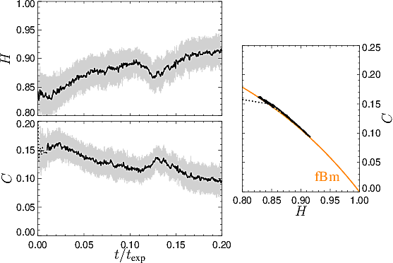
Figure 10: Evolution of (left top) the permutation entropy $H$ and (left bottom) the statistical complexity $C$ of $B_{y}$ component of the magnetic field calculated at about $45^{\mathrm{o}}$ with respect to the ambient magnetic field as functions of time (mean values shown in black whereas the gray area denote the mean values $\pm$ the standard deviation; dotted lines denote an initial transition phase). (right) Mean simulation data in the $(H,C)$ plane (black line) compared to the prediction for the fractional Brownian motion (orange line); dotted line denotes the initial transient phase.

4 Discussion & Conclusion

In this paper we used the 3-D HEB simulation to investigate properties of the turbulent cascade and its relationship with fire hose instabilities. We initialized the system with an isotropic spectrum of (relatively) large-scale Alfvénic fluctuations having zero cross-helicity. Nonlinear coupling of these modes leads to a turbulent cascade and energization of protons. Such energization is not, however, strong enough to compete with the anisotropic cooling due to the expansion and protons develop an important parallel ($T_{\perp}<T_{\|}$) temperature anisotropy similar to in situ observations from Helios spacecraft (Matteini et al., 2007); larger-amplitude turbulent fluctuations are needed to counterbalance the solar wind expansion (cf., Montagud-Camps et al., 2018). When the proton temperature anisotropy becomes strong enough, parallel and oblique fire hoses are destabilized and generate quasi-coherent wave packets with an amplitude much smaller than that of the background turbulence. The generated waves efficiently reduce the proton temperature anisotropy, they are partly reabsorbed by protons through cyclotron resonances and partly couple to and participate in the turbulent cascade. Turbulent fluctuations shape the plasma system, leading to the formation of variable electromagnetic field as well as variable proton density, temperature anisotropy, agyrotropy, etc. The fire hose wave activity reduces the proton temperature anisotropy while it further increases the proton agyrotropy. Despite the inhomogeneity/nonuniformity and agyrotropy of the plasma system, the linear prediction based on the corresponding homogeneous and uniform gyrotropic approximation is in a semi-quantitative agreement with the simulation results.

In the 2-D HEB simulation of Hellinger et al. (2015) the expansion-driven fire hose fluctuations are by construction injected to the turbulent cascade; they are forced to have wave vectors perpendicular to the ambient magnetic field where the cascade proceeds. In this case, the simulation results indicate that the growth rate of unstable modes must be strong enough to compete with the cascade characterized by the nonlinear eddy turn-over time $t_{nl}$. In the real space, the fire hose fluctuations were strongly localized in the 2-D simulation between magnetic islands and tend to be aligned along the local most uniform direction. In the 3-D simulation the fire hose fluctuations appear to be outside the region dominated by the turbulent cascade; their wave vectors are quasi-parallel/oblique with respect to the ambient magnetic field and lie outside of the region in the wave vector space $(k_{\|},k_{\perp})$ dominated by the turbulent cascade. In this quasi-parallel/oblique region the nonlinear eddy turn-over time ($t_{nl}\propto 1/\delta B$) is long so that it does not present a large obstacle to the development of the instabilities. In the real space, the fluctuations have quasi-parallel/oblique propagation and are directed about along the ambient magnetic field (magnetic field-lines) that constitutes also roughly the most uniform direction. We are inclined to speculate that the presence of the turbulent cascade has a tendency to push the unstable modes outside the region dominated by the cascade. More work is needed to test it.

The well-developed turbulence in the 3-D simulation before the onset of the fire hose instabilities exhibit anisotropic intermittency properties that correspond to the anisotropic cascade. The kurtosis depends strongly on the separation scale $l_{\perp}$ perpendicular to the ambient magnetic field (similar results are obtained also for the standard 3-D hybrid simulation of Franci et al., 2018b). The kurtosis saturates and decreases for scales $l_{\perp}\lesssim d_{i}$ and is weaker at the quasi-parallel direction $l_{\|}>l_{\perp}$. The reduction of the kurtosis is likely related to the (resistive) dissipation, a relatively large resistivity is used to avoid the accumulation of the magnetic energy on small scales. The weak fire hose wave activity affects the kurtosis and leads to its reduction at the quasi-parallel directions; the generated waves have likely rather Gaussian character which leads to a reduction of kurtosis; however, because of their weak amplitude, they do not affect significantly the statistical properties of fluctuations at oblique angles where the turbulent fluctuations dominate.

For the developed turbulence in the presented simulation before the onset of the fire hose instabilities the Shannon entropy $H$ and the Jensen-Shannon complexity $C$ comparable to in situ observations in the solar wind (Weck et al., 2015; Weygand & Kivelson, 2019), $H$ increases and $C$ increases with the time (corresponding to the radial distance) as expected (and observed in a simulation where the fire hose instabilities are not generated) and they follow the prediction for a fractional Brownian motion in the $(H,C)$ plane similarly to the observational results of Weygand & Kivelson (2019). The fire hose wave activity brings new information to the system and causes a decreases of the entropy $H$ and to an increase of the complexity $C$ as may be expected. Interestingly, even when the fire hose waves are present, $H$ and $C$ keep following the prediction for a fractional Brownian motion. However, the meaning of $H$ and $C$ (and their connection to the fractional Brownian motion) are yet to be understood.

This wave activity is easily identified as a narrow peak on top of the background turbulence in 1-D power spectra similar to observations but only at quasi-parallel/oblique angles with respect to the ambient magnetic field. For more oblique angles, the fire hose wave activity is not discernible because of its low amplitude compared to the turbulent background. We expect a similar behavior for in situ observations. In this case it may be possible to detect the wave activity based on the coherence property (Lion et al., 2016). Furthermore, as the instability-driven wave activity modifies the statistical properties of the turbulent fluctuations, one may ask if these quantities may be used to discern generation of a (quasi-coherent) wave activity (such as instability-driven waves) within a turbulent system. It seems that the intermittency/kurtosis is not very useful in this respect, as it is only reduced in the quasi-parallel direction. The Shannon entropy and the Jensen-Shannon complexity are more promising tools; in contrast to the kurtosis, they don’t seem to be strongly dependent on the angle the time series are measured with respect to the ambient magnetic field. However, it is unclear whether they can be used for real observations, since the change of two quantities in the simulation is rather weak.

The present 3-D simulation has many limitations. We used parameters similar to the 2D case of Hellinger et al. (2015) with an expansion about ten times faster than in the solar wind. At the same time, the amplitude of the turbulent fluctuations were larger so that the ratio between the expansion and turbulence characteristic time scales is comparable to that observed in the solar wind. The fire hose driven magnetic fluctuations reach a relatively low amplitude with respect to the ambient turbulence but they are efficient in reducing the proton temperature anisotropy owing to the resonant character of their interaction with protons. For a realistic expansion time we expect even a weaker level of fluctuations (Matteini et al., 2006; Hellinger, 2017); the realistic level of turbulent fluctuation is also lower so that we expect a similar relative amplitude of fire hose and turbulent fluctuations in the solar wind. A probably more important limitation of the present results is the size of the simulation box. Due to the limited resources we have a relatively small box size and we initially inject the energy at relatively small scales compared to the solar wind conditions. Consequently, the level of intermittency observed in the simulation is relatively weak. Its formation on small scales is also possibly reduced by noise due to the limited number of particles per cell.

Despite these limitations, our numerical results show that fire hose instabilities coexist with plasma turbulence and generate temperature-anisotropy reducing modes that lie in the spectral space outside the region dominated by the turbulent cascade. We expect a similar behavior for other ion kinetic instabilities driven by particle temperature anisotropies and/or differential streaming in the solar wind (as indicated by in situ observations of Klein et al., 2018), except possibly for the mirror instability that drives strongly oblique modes; 2-D numerical simulations show that the mirror instability coexists with plasma turbulence (Hellinger et al., 2017). However, the present simulation results show that these 2-D results are too limited and need to be revisited.

References

- Alexandrova et al. (2008) Alexandrova, O., Carbone, V., Veltri, P., & Sorriso-Valvo, L. 2008, ApJ, 674, 1153, doi:10.1086/524056
- Alexandrova et al. (2013) Alexandrova, O., Chen, C. H. K., Sorriso-Valvo, L., Horbury, T. S., & Bale, S. D. 2013, Space Sci. Rev., 178, 101, doi:10.1007/s11214-013-0004-8
- Arzamasskiy et al. (2019) Arzamasskiy, L., Kunz, M. W., Chandran, B. D. G., & Quataert, E. 2019, ApJ, 879, 53, doi:10.3847/1538-4357/ab20cc
- Bandt & Pompe (2002) Bandt, C., & Pompe, P. 2002, PhRvL, 88, 174102
- Bandt & Shiha (2007) Bandt, C., & Shiha, F. 2007, J. Time Ser. Analysis, 28, 646, doi:10.1111/j.1467-9892.2007.00528.x
- Bruno & Carbone (2013) Bruno, R., & Carbone, V. 2013, LRSP, 10, 2, doi:10.12942/lrsp-2013-2
- Cranmer et al. (2009) Cranmer, S. R., Matthaeus, W. H., Breech, B. A., & Kasper, J. C. 2009, ApJ, 702, 1604, doi:10.1088/0004-637X/702/2/1604
- Del Sarto & Pegoraro (2018) Del Sarto, D., & Pegoraro, F. 2018, MNRAS, 475, 181, doi:10.1093/mnras/stx3083
- Dong et al. (2014) Dong, Y., Verdini, A., & Grappin, R. 2014, ApJ, 793, 118, doi:10.1088/0004-637X/793/2/118
- Franci et al. (2018a) Franci, L., Hellinger, P., Guarrasi, M., et al. 2018a, J. Phys.: Conf. Ser., 1031, 012002, doi:10.1088/1742-6596/1031/1/012002
- Franci et al. (2015) Franci, L., Landi, S., Matteini, L., Verdini, A., & Hellinger, P. 2015, ApJ, 812, 21, doi:10.1088/0004-637X/812/1/21
- Franci et al. (2018b) Franci, L., Landi, S., Verdini, A., Matteini, L., & Hellinger, P. 2018b, ApJ, 1, 26, doi:10.3847/1538-4357/aaa3e8
- Gary (1993) Gary, S. P. 1993, Theory of Space Plasma Microinstabilities (New York: Cambridge Univ. Press)
- Gary et al. (2001) Gary, S. P., Goldstein, B. E., & Steinberg, J. T. 2001, JGR, 106, 24955
- Gary et al. (2016) Gary, S. P., Jian, L. K., Broiles, T. W., et al. 2016, JGR, 121, 30, doi:10.1002/2015JA021935
- Gary et al. (1998) Gary, S. P., Li, H., O’Rourke, S., & Winske, D. 1998, JGR, 103, 14567
- Grappin et al. (1993) Grappin, R., Velli, M., & Mangeney, A. 1993, PhRvL, 70, 2190
- Hellinger (2017) Hellinger, P. 2017, JPlPh, 83, 705830105, doi:10.1017/S0022377817000071
- Hellinger et al. (2017) Hellinger, P., Landi, S., Matteini, L., Verdini, A., & Franci, L. 2017, ApJ, 838, 158, doi:10.3847/1538-4357/aa67e0
- Hellinger & Matsumoto (2000) Hellinger, P., & Matsumoto, H. 2000, JGR, 105, 10519
- Hellinger & Matsumoto (2001) —. 2001, JGR, 106, 13215
- Hellinger et al. (2015) Hellinger, P., Matteini, L., Landi, S., et al. 2015, ApJL, 811, L32, doi:10.1088/2041-8205/811/2/L32
- Hellinger & Trávníček (2005) Hellinger, P., & Trávníček, P. 2005, JGR, 110, A04210, doi:10.1029/2004JA010687
- Hellinger & Trávníček (2008) —. 2008, JGR, 113, A10109, doi:10.1029/2008JA013416
- Hellinger et al. (2006) Hellinger, P., Trávníček, P., Kasper, J. C., & Lazarus, A. J. 2006, GeoRL, 33, L09101, doi:10.1029/2006GL025925
- Hellinger et al. (2013) Hellinger, P., Trávníček, P. M., Štverák, Š., Matteini, L., & Velli, M. 2013, JGR, 118, 1351, doi:10.1002/jgra.50107
- Jian et al. (2009) Jian, L. K., Russell, C. T., Luhmann, J. G., et al. 2009, ApJL, 701, L105, doi:10.1088/0004-637X/701/2/L105
- Klein et al. (2018) Klein, K. G., Alterman, B. L., Stevens, M. L., Vech, D., & Kasper, J. C. 2018, PhRvL, 120, 205102, doi:10.1103/PhysRevLett.120.205102
- Klein & Howes (2015) Klein, K. G., & Howes, G. G. 2015, PhPl, 22, 032903, doi:10.1063/1.4914933
- Lamberti et al. (2004) Lamberti, P. W., Martin, M. T., Plastino, A., & Rosso, O. A. 2004, Phys. A, 334, 119
- Lion et al. (2016) Lion, S., Alexandrova, O., & Zaslavsky, A. 2016, ApJ, 824, 47, doi:10.3847/0004-637X/824/1/47
- López-Ruiz et al. (1995) López-Ruiz, R., Mancini, H. L., & Calbet, X. 1995, Phys. Lett. A, 209, 321, doi:10.1016/0375-9601(95)00867-5
- MacBride et al. (2008) MacBride, B. T., Smith, C. W., & Forman, M. A. 2008, ApJ, 679, 1644, doi:10.1086/529575
- Maggs & Morales (2013) Maggs, J. E., & Morales, G. J. 2013, Plasma Phys. Control. Fusion, 55, 085015, doi:10.1088/0741-3335/55/8/085015
- Markovskii & Vasquez (2011) Markovskii, S. A., & Vasquez, B. J. 2011, ApJ, 739, 22, doi:10.1088/0004-637X/739/1/22
- Maruca et al. (2012) Maruca, B. A., Kasper, J. C., & Gary, S. P. 2012, ApJ, 748, 137, doi:10.1088/0004-637X/748/2/137
- Matteini et al. (2013) Matteini, L., Hellinger, P., Goldstein, B. E., et al. 2013, JGR, 118, 2771, doi:10.1002/jgra.50320
- Matteini et al. (2012) Matteini, L., Hellinger, P., Landi, S., Trávníček, P. M., & Velli, M. 2012, Space Sci. Rev., 172, 373, doi:10.1007/s11214-011-9774-z
- Matteini et al. (2007) Matteini, L., Landi, S., Hellinger, P., et al. 2007, GeoRL, 34, L20105, doi:10.1029/2007GL030920
- Matteini et al. (2006) Matteini, L., Landi, S., Hellinger, P., & Velli, M. 2006, JGR, 111, A10101, doi:10.1029/2006JA011667
- Matthaeus & Velli (2011) Matthaeus, W. H., & Velli, M. 2011, Space Sci. Rev., 160, 145, doi:10.1007/s11214-011-9793-9
- Matthaeus et al. (2015) Matthaeus, W. H., Wan, M., Servidio, S., et al. 2015, Phil. Trans. R. Soc. A, 373, 20140154, doi:10.1098/rsta.2014.0154
- Matthews (1994) Matthews, A. 1994, JCoPh, 112, 102
- Mininni & Pouquet (2009) Mininni, P. D., & Pouquet, A. 2009, PhRvE, 80, 025401, doi:10.1103/PhysRevE.80.025401
- Montagud-Camps et al. (2018) Montagud-Camps, V., Grappin, R., & Verdini, A. 2018, ApJ, 853, 153, doi:10.3847/1538-4357/aaa1ea
- Ofman (2019) Ofman, L. 2019, Sol. Phys., 294, 51, doi:10.1007/s11207-019-1440-8
- Olivier et al. (2019) Olivier, C. P., Engelbrecht, N. E., & Strauss, R. D. 2019, JGR, 124, 4, doi:10.1029/2018JA026102
- Oughton et al. (1994) Oughton, S., Priest, E. R., & Matthaeus, W. H. 1994, J. Fluid Mech., 280, 95, doi:10.1017/S0022112094002867
- Papini et al. (2019) Papini, E., Franci, L., Landi, S., et al. 2019, ApJ, 870, 52, doi:10.3847/1538-4357/aaf003
- Parashar et al. (2018) Parashar, T. N., Matthaeus, W. H., & Shay, M. A. 2018, ApJL, 864, L21, doi:10.3847/2041-8213/aadb8b
- Parashar et al. (2009) Parashar, T. N., Shay, M. A., Cassak, P. A., & Matthaeus, W. H. 2009, PhPl, 16, 032310, doi:10.1063/1.3094062
- Petrosyan et al. (2010) Petrosyan, A., Balogh, A., Goldstein, M. L., et al. 2010, Space Sci. Rev., 156, 135, doi:10.1007/s11214-010-9694-3
- Scudder & Daughton (2008) Scudder, J., & Daughton, W. 2008, JGR, 113, A06222, doi:10.1029/2008JA013035
- Servidio et al. (2015) Servidio, S., Valentini, F., Perrone, D., et al. 2015, JPlPh, 81, 325810107, doi:10.1017/S0022377814000841
- Shebalin et al. (1983) Shebalin, J. V., Matthaeus, W. H., & Montgomery, D. 1983, JPlPh, 29, 525
- Stansby et al. (2019) Stansby, D., Perrone, D., Matteini, L., Horbury, T. S., & Salem, C. S. 2019, A&A, 623, L2, doi:10.1051/0004-6361/201834900
- Štverák et al. (2015) Štverák, Š., Trávníček, P. M., & Hellinger, P. 2015, JGR, 120, 8177, doi:10.1002/2015JA021368
- Valentini et al. (2014) Valentini, F., Servidio, S., Perrone, D., et al. 2014, PhPl, 21, 082307, doi:10.1063/1.4893301
- Verdini & Grappin (2015) Verdini, A., & Grappin, R. 2015, ApJL, 808, L34, doi:10.1088/2041-8205/808/2/L34
- Verdini et al. (2015) Verdini, A., Grappin, R., Hellinger, P., Landi, S., & Müller, W. C. 2015, ApJ, 804, 119, doi:10.1088/0004-637X/804/2/119
- Weck et al. (2015) Weck, P. J., Schaffner, D. A., Brown, M. R., & Wicks, R. T. 2015, PhRvE, 91, 23101, doi:10.1103/PhysRevE.91.023101
- Weygand & Kivelson (2019) Weygand, J. M., & Kivelson, M. G. 2019, ApJ, 872, 59, doi:10.3847/1538-4357/aafda4
- Wicks et al. (2016) Wicks, R. T., Alexander, R. L., Stevens, M., et al. 2016, ApJ, 819, 6, doi:10.3847/0004-637X/819/1/6
- Wu et al. (2013) Wu, P., Wan, M., Matthaeus, W. H., Shay, M. A., & Swisdak, M. 2013, PhRvL, 111, 121105, doi:10.1103/PhysRevLett.111.121105
- Zunino et al. (2008) Zunino, L., Pérez, D. G., Martín, M. T., et al. 2008, Phys. Lett. A, 372, 4768, doi:10.1016/j.physleta.2008.05.026