Abstract

The discovery of a non-zero rate for a lepton flavor violating decay mode of the Higgs boson would definitely be an indication of New Physics. We review the prospects for such signal in Two Higgs Doublet Models, in particular for Higgs boson decays into $\tau\mu$ final states. We will show that this scenario contains all the necessary ingredients to provide large flavor violating rates and still be compatible with the stringent limits from direct searches and low-energy flavor experiments.

1 Introduction

The discovery of the Higgs boson in 2012 at the LHC by the ATLAS and CMS collaborations constitutes a historical milestone for particle physics and another brilliant triumph for the Standard Model (SM). With this long-awaited completion of the SM particle spectrum, it stands as one of the most successful theories ever built, providing precise predictions for a wide range of particle physics phenomena, in good agreement with a large amount of experimental results at low and high energies.

Despite this remarkable success, many fundamental questions remain unanswered in the SM. The list is long and contains experimental observations that cannot be addressed in the SM and theoretical issues that cannot be fully understood in its context. It includes the origin of neutrino masses, the nature of dark matter, the conservation of CP in the strong interactions or the reason for the replication of fermion generations, to mention a few. These open problems clearly call for an extension of the SM with new states, presumably present at high energies, and/or new dynamics.

New Physics (NP) may manifest in the form of Higgs boson properties different from those predicted by the SM. For this reason, it is crucial to look for deviations in the Higgs couplings to fermions and gauge bosons and the Higgs boson total decay width or the existence of new Higgs decay channels. In particular, new degrees of freedom coupling to the SM leptons and the Higgs boson could induce non-zero lepton flavor violating (LFV) Higgs boson decays, such as $h\to\ell_{i}\ell_{j}$ with $i\neq j$, indeed a common feature in many models with extended scalar or lepton sectors. The observation of these processes, strictly forbidden in the SM, would provide a clear hint of NP at work.

Higgs lepton flavor violating (HLFV) signatures face many indirect constraints, since most of the NP scenarios that lead to them modify other Higgs properties as well, some already experimentally determined to lie close to the SM prediction. Moreover, HLFV signatures typically come along with other LFV processes, such as the $\ell_{i}\to\ell_{j}\gamma$ radiative decays. While model-independent studies [1, 2, 3, 4, 5, 6] have shown that large HLFV rates are in principle compatible with the existing experimental constraints, this is not generally the case in specific models. In fact, most models predict HLFV rates below the current LHC sensitivity. In contrast, the Two Higgs Doublet Model (2HDM) [7, 8] has been shown to be able to accommodate large $h\to\ell_{i}\ell_{j}$ branching ratios [9], clearly within the reach of the ATLAS and CMS detectors.

This minireview focuses on HLFV in the 2HDM. Several pioneer works already addressed HLFV in the pre-LHC era [10, 11, 12, 13, 14, 15, 16, 17, 18], and many have revisited the subject in the context of the 2HDM [19, 20, 21] or in other contexts [22, 23, 24, 25, 26, 27, 28] after the LHC has started delivering data. In fact, early results by the CMS collaboration hinted at a non-zero $h\to\tau\mu$ branching ratio [29], and this raised a considerable attention in the community, leading to many works [9, 30, 31, 32, 33, 34, 35, 36, 37, 38, 39, 40, 41, 42, 43, 44, 45, 46, 47, 48, 49, 50, 51, 52, 53, 54, 55, 56, 57, 58, 59, 60, 61, 62, 63, 64, 65, 66, 67, 68, 69, 70, 71, 72, 73, 74, 75, 76, 77, 78, 79, 80, 81, 82, 83, 84, 85, 86, 87, 88, 89, 90, 91]. We will first follow some general model-independent arguments that identify the 2HDM as a scenario with potentially large HLFV signatures and later highlight some selected phenomenological results on HLFV in the 2HDM. Even though the theoretical discussion will be general and not concentrate on any particular combination of lepton flavors, we will focus on $\tau\mu$ LFV in the phenomenological discussion.

The rest of the manuscript is structured as follows. In Sec. 2 the current experimental bounds for the rates of several LFV processes, including $h\to\ell_{i}\ell_{j}$, are briefly discussed. Sec. 3 contains general model-independent considerations, while Sec. 4 argues that a type-III 2HDM may accommodate sizable $h\to\ell_{i}\ell_{j}$ branching ratios and makes this point explicitly after introducing our 2HDM notation and conventions. Finally, we comment on some 2HDM scenarios that generate neutrino masses and may lead to large HLFV rates in Sec. 5 and conclude in Sec. 6.

2 Experimental status

HLFV Decay BR	ATLAS	CMS
$h\to\mu e$	$6.1\times 10^{-5}$ [92]	$3.5\times 10^{-4}$ [93]
$h\to\tau\mu$	$2.8\times 10^{-3}$  [94]	$2.5\times 10^{-3}$ [95]
$h\to\tau e$	$4.7\times 10^{-3}$ [94]	$6.1\times 10^{-3}$ [95]

Table 1: Experimental $95~{}\%$ C.L. upper bounds on HLFV branching ratios from the ATLAS and CMS collaborations.

A remarkable effort has been devoted to the search for LFV in processes involving charged leptons, resulting in impressive bounds in some channels. This has been particularly well motivated after the discovery of neutrino flavor oscillations, which imply that charged lepton flavor violating processes must exist, although perhaps with low rates.

In what concerns HLFV, the ATLAS and CMS collaborations have searched for $h\to\ell_{i}\ell_{j}$, setting limits for the corresponding branching ratios in the $10^{-5}-10^{-3}$ ballpark, as shown in Tab. 1.  The CMS limit on $\text{BR}(h\to\mu e)$ has been obtained using $\sqrt{s}=8$ TeV data, whereas the rest of ATLAS and CMS limits have been updated including $\sqrt{s}=13$ TeV data. Dedicated strategies can in principle improve these limits substantially with future LHC data [3], in particular in the 14 TeV HL-LHC phase [63]. Furthermore, HLFV can also be searched for at $e^{+}e^{-}$ colliders, which offer a very clean environment, perfectly suited for the exploration of the Higgs boson properties. As shown by several analyses [63, 66, 86, 87], the planned future $e^{+}e^{-}$ facilities (CEPC, FCC-ee and ILC) can probe HLFV branching ratios as low as $10^{-5}-10^{-4}$, improving on the current LHC limits by about one order of magnitude for channels involving the $\tau$ lepton.

LFV Process BR	Present Bound	Future Sensitivity
$\mu\to e\gamma$	$4.2\times 10^{-13}$ [96]	$6\times 10^{-14}$ [97]
$\tau\to e\gamma$	$3.3\times 10^{-8}$ [98]	$\sim 3\times 10^{-9}$ [99]
$\tau\to\mu\gamma$	$4.4\times 10^{-8}$ [98]	$\sim 3\times 10^{-9}$ [99]
$\mu\rightarrow eee$	$1.0\times 10^{-12}$ [100]	$\sim 10^{-16}$ [101]
$\tau\rightarrow eee$	$2.7\times 10^{-8}$ [102]	$\sim 10^{-9}$ [99]
$\tau\rightarrow\mu\mu\mu$	$2.1\times 10^{-8}$ [102]	$\sim 10^{-9}$ [99]
$\tau^{-}\rightarrow e^{-}\mu^{+}\mu^{-}$	$2.7\times 10^{-8}$ [102]	$\sim 10^{-9}$ [99]
$\tau^{-}\rightarrow\mu^{-}e^{+}e^{-}$	$1.8\times 10^{-8}$ [102]	$\sim 10^{-9}$ [99]
$\tau^{-}\rightarrow e^{+}\mu^{-}\mu^{-}$	$1.7\times 10^{-8}$ [102]	$\sim 10^{-9}$ [99]
$\tau^{-}\rightarrow\mu^{+}e^{-}e^{-}$	$1.5\times 10^{-8}$ [102]	$\sim 10^{-9}$ [99]
$\mu^{-},\mathrm{Ti}\rightarrow e^{-},\mathrm{Ti}$	$4.3\times 10^{-12}$ [103]	$\sim 10^{-18}$ [104]
$\mu^{-},\mathrm{Au}\rightarrow e^{-},\mathrm{Au}$	$7\times 10^{-13}$ [105]
$\mu^{-},\mathrm{Al}\rightarrow e^{-},\mathrm{Al}$		$10^{-15}-10^{-18}$ [106]
$\mu^{-},\mathrm{SiC}\rightarrow e^{-},\mathrm{SiC}$		$10^{-14}$ [107]

Table 2: Current experimental bounds and future sensitivities for several LFV observables of interest.

The NP degrees of freedom and interactions leading to $h\to\ell_{i}\ell_{j}$ also generate other LFV processes, such as $\ell_{i}\to\ell_{j}\gamma$. Since these are subject to much stronger experimental bounds, they tend to be crucial constraints in most specific models and must be considered in any phenomenological study on HLFV decays. Tab. 2 collects the current bounds and future sensitivities for several LFV processes of interest. Muon LFV observables have the best experimental limits due to the existence of high-intensity muon beams, while the branching ratios for tau LFV decays are bound to be below $\sim 10^{-8}$. The most constraining processes in many models are the $\ell_{i}\to\ell_{j}\gamma$ radiative decays. The MEG collaboration has established the strong limit $\text{BR}(\mu\to e\gamma)<4.2\cdot 10^{-13}$, a bound that will be improved by about an order of magnitude in the MEG-II phase [97]. Regarding the $\ell_{i}\to\ell_{j}\ell_{k}\ell_{k}$ 3-body decays, the $\mu\to eee$ branching ratio sensitivity is expected to be improved by four orders of magnitude by the Mu3e experiment [101]. Finally, the most spectacular progress in the search for LFV are expected in $\mu-e$ conversion experiments, which are also expected to improve the current limits for different nuclei by several orders of magnitude [104, 106, 107]. See [108] for an experimental and theoretical review of the current situation in charged lepton flavor violation experiments.

3 Model-independent considerations

In order to explore HLFV in a model-independent way, it proves convenient to adopt an approach based on Effectively Field Theory (EFT). This is particularly well motivated due to lack of NP signals at the LHC, which arguably implies that any new particles responsible for HLFV would lie clearly above the electroweak scale. We will now continue along the lines of [72]. 

In addition to canonical kinetic terms, the SM Lagrangian contains the Yukawa terms for the leptons

$$-\mathcal{L}_{\rm SM}^{Y}=\bar{\ell}\,\Gamma_{e}\,e\,\varphi+\text{h.c.}\,,$$ (1)

where

$$\ell=\left(\begin{array}[]{c}\nu\\ e\end{array}\right)_{L}\sim\left({\bf 1},{\bf 2},-\frac{1}{2}\right)\,,\quad e\equiv e_{R}\sim\left({\bf 1},{\bf 1},-1\right)\quad\text{and}\quad\varphi=\left(\begin{array}[]{c}\varphi^{+}\\ \varphi^{0}\end{array}\right)\sim\left({\bf 1},{\bf 2},\frac{1}{2}\right)$$ (6)

denote the SM lepton $\rm SU(2)_{L}$ doublets and singlets and Higgs doublet, respectively, and we give the representation under the SM gauge group $\rm SU(3)_{c}\times SU(2)_{L}\times U(1)_{Y}$. $\Gamma_{e}$ is a $3\times 3$ complex matrix that can be taken to be diagonal without loss of generality. Therefore, the three lepton flavors are exactly conserved in the SM, which then possesses a $G_{f}=\rm{U(1)_{e}\times U(1)_{\mu}\times U(1)_{\tau}}$ global flavor symmetry. 

The flavor symmetry $G_{f}$ gets generally broken in the presence of NP. This can be generically parametrized by means of non-renormalizable gauge-invariant operators of dimension $d>4$ that encode the LFV effects induced by unknown heavy states,

$$\mathcal{L}_{\rm EFT}=\frac{C_{i}}{\Lambda^{d-4}}\,Q_{i}+\text{h.c.}\,.$$ (7)

Here $\Lambda$ is the scale of NP, of the order of the masses of the states whose decoupling induces the dimension-$d$ operator $Q_{i}$, and $C_{i}$ the associated Wilson coefficient. There are many of such LFV operators. However, the only dimension-six operator giving rise to Higgs LFV is $Q_{e\varphi}$, defined as

$$Q_{e\varphi}=\left(\varphi^{\dagger}\varphi\right)\,\left(\bar{\ell}\,e\,\varphi\right)\,.$$ (8)

This operator was first highlighted in the context of HLFV in [3], later denoted the Yukawa operator in [72] and is one of the operators in the Warsaw basis of the Standard Model Effective Field Theory [110].  Any additional gauge-invariant dimension-six operator leading to HLFV can be shown to be redundant, and therefore reducible to $Q_{e\varphi}$ by using equations of motion, Fierz transformations or other field redefinitions [3]. Therefore, all HLFV effects are encoded (at least in scenarios leading to NP contributions of dimension six) by $Q_{e\varphi}$.

After electroweak symmetry breaking, the SM Yukawa term in Eq. (1) and the NP contribution encoded in $Q_{e\varphi}$ add up to

$$\mathcal{L}_{\rm SM}^{Y}+\mathcal{L}_{\rm EFT} \supset-\,\bar{e}_{L}\left[\frac{v}{\sqrt{2}}\,\left(\Gamma_{e}-C_{e\varphi}\,\frac{v^{2}}{2\Lambda^{2}}\right)+\frac{h}{\sqrt{2}}\,\left(\Gamma_{e}-3\,C_{e\varphi}\,\frac{v^{2}}{2\Lambda^{2}}\right)\right]e_{R}+\text{h.c.}$$

$$=-\,\bar{e}_{L}\left[\mathcal{M}_{e}+h\,\mathcal{Y}_{e}\right]e_{R}+\text{h.c.}\,,$$ (9)

where

$$\mathcal{M}_{e}=\frac{v}{\sqrt{2}}\,\left(\Gamma_{e}-C_{e\varphi}\,\frac{v^{2}}{2\Lambda^{2}}\right)$$ (10)

is the $3\times 3$ charged lepton mass matrix and

$$\mathcal{Y}_{e}=\frac{1}{\sqrt{2}}\,\left(\Gamma_{e}-3\,C_{e\varphi}\,\frac{v^{2}}{2\Lambda^{2}}\right)$$ (11)

are the Higgs boson couplings to a pair of charged leptons. We have used the decomposition $\varphi^{0}=\frac{1}{\sqrt{2}}(h+i\,G^{0}+v)$, with $h$ the physical Higgs boson with a mass $m_{h}\simeq 125$ GeV, $G^{0}$ the Goldstone boson that constitutes the longitudinal component of the massive $Z$-boson and $v\simeq 246$ GeV the electroweak vacuum expectation value (VEV). It is clear that, in general, the matrices $\mathcal{M}_{e}$ and $\mathcal{Y}_{e}$ are not diagonal in the same basis. In fact, in the mass basis, defined by

$$V_{e_{L}}^{\dagger}\mathcal{M}_{e}V_{e_{R}}=\widehat{\mathcal{M}}_{e}=\text{diag}(m_{e},m_{\mu},m_{\tau})\,,$$ (12)

the Higgs boson couplings to charged leptons read

$$g_{h\ell\ell}=V_{e_{L}}^{\dagger}\mathcal{Y}_{e}V_{e_{R}}=\frac{1}{v}\,\widehat{\mathcal{M}}_{e}-\frac{v^{2}}{\sqrt{2}\Lambda^{2}}\,V_{e_{L}}^{\dagger}C_{e\varphi}V_{e_{R}}\,.$$ (13)

While the first term in Eq. (13) is proportional to the charged lepton masses, the second one can in general contain off-diagonal entries and induce HLFV processes. In particular, this piece leads to the $h\to\ell_{i}\ell_{j}$ decays, with $i\neq j$. One finds

$$\text{BR}(h\to\ell_{i}\ell_{j})=\frac{m_{h}}{8\pi\Gamma_{h}}\,\left(|g_{h\ell_{i}\ell_{j}}|^{2}+|g_{h\ell_{j}\ell_{i}}|^{2}\right)\,,$$ (14)

where $\Gamma_{h}$ ($\simeq 4$ MeV in the SM) is the total Higgs boson decay width.

So far, we only discussed the $Q_{e\varphi}$ operator, which induces the HLFV decays $h\to\ell_{i}\ell_{j}$ we are interested in. However, in a complete ultraviolet theory other operators will be generated as well. In particular, operators that give rise to other LFV processes, such as $\ell_{i}\to\ell_{j}\gamma$, with much stronger experimental bounds. At dimension six, two gauge-invariant operators of this type exist [110],

$$Q_{eW}=\left(\bar{\ell}\sigma^{\mu\nu}e\right)\tau^{I}\varphi\,W^{I}_{\mu\nu}\quad\text{and}\quad Q_{eB}=\left(\bar{\ell}\sigma^{\mu\nu}e\right)\varphi\,B_{\mu\nu}\,,$$ (15)

where $\tau^{I}$, with $I=1,2,3$, are the Pauli matrices. At low energies, these two operators are matched to the dimension-five photonic dipole operator 

$$\mathcal{O}_{e\gamma}=\bar{e}_{L}\sigma^{\mu\nu}e_{R}\,F_{\mu\nu}\,,$$ (16)

which is directly responsible for the $\ell_{i}\to\ell_{j}\gamma$ radiative LFV decays. Defining the contribution of $\mathcal{O}_{e\gamma}$ to the low-energy effective Lagrangian as

$$\mathcal{L}_{\rm EFT}^{\rm low}=\frac{L_{e\gamma}}{v}\,\mathcal{O}_{e\gamma}+\text{h.c.}\,,$$ (17)

where $L_{e\gamma}$ is its Wilson coefficient, the resulting branching ratios are

$$\text{BR}(\ell_{i}\to\ell_{j}\gamma)=\frac{m_{i}^{3}}{4\pi v^{2}\,\Gamma_{i}}\left(|\left(L_{e\gamma}\right)_{ij}|^{2}+|\left(L_{e\gamma}\right)_{ji}|^{2}\right)\,,$$ (18)

with $m_{i}$ and $\Gamma_{i}$ the mass and total decay width of the charged lepton $\ell_{i}$, respectively.

Any theory that induces $Q_{e\varphi}$ will also generate $\mathcal{O}_{e\gamma}$, since these operators transform in the same way under flavor and chiral symmetries [33] and mix under renormalization group evolution [113]. Therefore, one cannot simply get rid of the latter. However, different NP scenarios predict a different balance between the $C_{e\varphi}$ and $L_{e\gamma}$ Wilson coefficients, and this is what determines the magnitude of the allowed HLFV effects in a specific model. Let us consider an example to illustrate this connection: a model inducing predominantly $\left(Q_{eB}\right)_{12}$ at the high-energy scale $\Lambda$. In this case the operator $\left(Q_{e\varphi}\right)_{12}$ gets induced due to renormalization group running while $\left(\mathcal{O}_{e\gamma}\right)_{12}$ is obtained after matching at the electroweak scale. Since the HLFV operator is induced by operator mixing effects, the resulting coefficient is suppressed and one expects the relation $\text{BR}(h\to\mu e)\simeq 10^{-14}\,\log^{2}\left(m_{h}/\Lambda\right)\,\text{BR}(\mu\to e\gamma)$, which clearly precludes the observation of the HLFV decay. More generally, in models with $L_{e\gamma}\sim C_{e\varphi}$ or $L_{e\gamma}>C_{e\varphi}$, as in the example we just considered, the strong constraints derived from the non-observation of $\ell_{i}\to\ell_{j}\gamma$ would imply tiny HLFV rates. In contrast, models predicting $L_{e\gamma}\ll C_{e\varphi}$ may accommodate sizable HLFV effects. As we will see in Sec. 4.1, the 2HDM is one of such models.

4 HLFV in the 2HDM

We now concentrate on the 2HDM. First, in Sec. 4.1 we particularize the previous model-independent discussion to the case of a 2HDM in order to motivate this model as the perfect scenario to obtain large HLFV rates. Sec. 4.2 will introduce our notation and conventions for the 2HDM. Finally, we will concentrate on $\tau\mu$ flavor violation, discuss $\tau\to\mu\gamma$ in the 2HDM in Sec. 4.3 and show some selected phenomenological results on $h\to\tau\mu$ in the 2HDM in Sec. 4.4.

4.1 EFT motivation

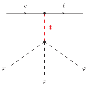
Figure 1: 2HDM ultraviolet completion of the $Q_{e\varphi}$ operator. Here $\Phi$ is a heavy new scalar $\rm SU(2)_{L}$ doublet. See [72] for details.

A NP model with a second scalar $\rm SU(2)_{L}$ doublet would induce the $Q_{e\varphi}$ operator, as shown in Fig. 1. This is one of the possible topologies contributing to the HLFV operator, as discussed in great detail in [72]. The scalar $\Phi$ must be an $\rm SU(2)_{L}$ doublet for the diagram to be gauge invariant, and would be identified with a second Higgs doublet in a 2HDM. Moreover, it should be noticed that this topology requires both scalar doublets to couple to leptons. The $\Phi$ coupling is clearly shown, and $\varphi$ was already assumed to couple to leptons, see Eq. (1). For this reason, the 2HDM behind the generation of this topology would be a type-III 2HDM, in which both Higgs doublets are allowed to couple to leptons in a general way. 

We note that $Q_{e\varphi}$ is generated at tree-level in this scenario, thus enhancing the Wilson coefficient $C_{e\varphi}$. We expect

$$\frac{C_{e\varphi}}{\Lambda^{2}}\sim\frac{\lambda\,y_{\Phi}}{m_{\Phi}^{2}}\,,$$ (19)

where $\lambda$ and $y_{\Phi}$ are the quartic scalar and Yukawa couplings involved in the topology shown in Fig. 1 and $m_{\Phi}$ the $\Phi$ scalar mass term. Next, we consider the generation of $\mathcal{O}_{e\gamma}$. This operator can be generated by attaching one of the external $\varphi$ lines in Fig. 1 to a charged lepton line and then adding the photon. There are, however, three effects that suppress the generation of this operator in the 2HDM:

• The $\mathcal{O}_{e\gamma}$ operator gets induced at the 1-loop level.

• Closing the loop by attaching the $\varphi$ line to the charged lepton line introduces a charged lepton mass insertion.

• The $\mathcal{O}_{e\gamma}$ operator requires a chirality flip, which in a SM extension with only new scalar fields (such as the 2HDM) implies an additional charged lepton mass insertion.

These considerations allow us to estimate

$$\left(L_{e\gamma}\right)_{ij}\sim\left(\frac{m_{i}}{v}\right)^{2}\,\frac{1}{16\,\pi^{2}}\,\left(C_{e\varphi}\right)_{ij}\ll\left(C_{e\varphi}\right)_{ij}\,.$$ (20)

This estimate is known to be very poor due to the presence of several additional contributions in a complete 2HDM, as we will show in Sec. 4.4. Nevertheless, it serves as a good motivation to consider this scenario as potentially promising in what concerns HLFV, since the required hierarchy between $C_{e\varphi}$ and $L_{e\gamma}$ is naturally obtained.

4.2 2HDM: model basics

In the following, we consider the general 2HDM, usually referred to as type-III 2HDM, and denote the two Higgs doublets as $\varphi_{1}$ and $\varphi_{2}$. In contrast to other variants of the 2HDM, no distinction between the two Higgs doublets is introduced. This has two consequences for our discussion. First, both $\varphi_{1}$ and $\varphi_{2}$ are allowed to couple to all fermion species, and in particular to leptons, a fundamental ingredient for the generation of HLFV effects, see Sec. 4.1. And second, one can perform arbitrary $\rm U(2)$ basis transformations in $\{\varphi_{1},\varphi_{2}\}$ space, without any impact on physical observables. This freedom can be used to go to a specific basis in which only one Higgs doublet acquires a VEV, the so-called Higgs basis [117, 118, 119]. In this basis, the scalar potential of the model is given by 

$$\mathcal{V} =\,M_{11}^{2}\,\varphi_{1}^{\dagger}\varphi_{1}+M_{22}^{2}\,\varphi_{2}^{\dagger}\varphi_{2}-\left(M_{12}^{2}\,\varphi_{1}^{\dagger}\varphi_{2}+\text{h.c.}\right)$$

$$+\frac{\Lambda_{1}}{2}\left(\varphi_{1}^{\dagger}\varphi_{1}\right)^{2}+\frac{\Lambda_{2}}{2}\left(\varphi_{2}^{\dagger}\varphi_{2}\right)^{2}+\Lambda_{3}\left(\varphi_{1}^{\dagger}\varphi_{1}\right)\left(\varphi_{2}^{\dagger}\varphi_{2}\right)+\Lambda_{4}\left(\varphi_{1}^{\dagger}\varphi_{2}\right)\left(\varphi_{2}^{\dagger}\varphi_{1}\right)$$

$$+\left[\frac{\Lambda_{5}}{2}\left(\varphi_{1}^{\dagger}\varphi_{2}\right)^{2}+\Lambda_{6}\left(\varphi_{1}^{\dagger}\varphi_{1}\right)\left(\varphi_{1}^{\dagger}\varphi_{2}\right)+\Lambda_{7}\left(\varphi_{2}^{\dagger}\varphi_{2}\right)\left(\varphi_{1}^{\dagger}\varphi_{2}\right)+\text{h.c.}\right]\,,$$ (21)

and the Higgs doublets can be decomposed as

$$\varphi_{1}=\left(\begin{array}[]{c}G^{+}\\ \frac{1}{\sqrt{2}}\left(v+\phi_{1}^{0}+i\,G^{0}\right)\end{array}\right)\quad,\quad\varphi_{2}=\left(\begin{array}[]{c}H^{+}\\ \frac{1}{\sqrt{2}}\left(\phi_{2}^{0}+i\,A\right)\end{array}\right)\,.$$ (22)

Here $\phi_{1}^{0}$, $\phi_{2}^{0}$ and $A$ are neutral scalars, $H^{+}$ is a charged scalar and $G^{+}$ and $G^{0}$ are Goldstone bosons. Assuming CP conservation, the CP-even states $\phi_{1}^{0}$ and $\phi_{2}^{0}$ do not mix with the CP-odd state $A$, which is a physical mass eigenstate. $\phi_{1}^{0}$ and $\phi_{2}^{0}$ are related to the mass eigenstates $h$ and $H$ (with $m_{h}<m_{H}$) as

$$\left(\begin{array}[]{c}h\\ H\end{array}\right)=\left(\begin{array}[]{cc}s_{\beta-\alpha}&c_{\beta-\alpha}\\ c_{\beta-\alpha}&-s_{\beta-\alpha}\end{array}\right)\,\left(\begin{array}[]{c}\phi_{1}^{0}\\ \phi_{2}^{0}\end{array}\right)\,,$$ (23)

where $s_{\beta-\alpha}\equiv\sin(\beta-\alpha)$, $c_{\beta-\alpha}\equiv\cos(\beta-\alpha)$ and $\beta-\alpha$ is a physical mixing angle. The lighest CP-even state, $h$, is identified with the Higgs boson discovered at the LHC. With these definitions at hand, one can derive several relations between the potential parameters and the physical Higgs masses [120],

$$m_{H^{+}}^{2} = M_{22}^{2}+\frac{v^{2}}{2}\Lambda_{3}\,,$$ (24)

$$m_{A}^{2}-m_{H^{+}}^{2} = -\frac{v^{2}}{2}\left(\Lambda_{5}-\Lambda_{4}\right)\,,$$ (25)

$$m_{H}^{2}+m_{h}^{2}-m_{A}^{2} = v^{2}\left(\Lambda_{1}+\Lambda_{5}\right)\,,$$ (26)

$$(m_{H}^{2}-m_{h}^{2})^{2} = \left[m_{A}^{2}+\left(\Lambda_{5}-\Lambda_{1}\right)v^{2}\right]^{2}+4\,\Lambda_{6}^{2}\,v^{4}\,,$$ (27)

$$\sin\left[2(\beta-\alpha)\right] = -\frac{2\,\Lambda_{6}\,v^{2}}{m_{H}^{2}-m_{h}^{2}}\,.$$ (28)

Let us now discuss the Yukawa interactions of the model. Again, we use the freedom to choose specific weak bases. In the Higgs basis for the scalar doublets and the mass basis for the fermions, the Yukawa Lagrangian can be written as

$$-\mathcal{L}_{\rm 2HDM}^{Y}= \,\frac{\sqrt{2}}{v}\,\left(\bar{q}\,K^{\ast}\,\widehat{\mathcal{M}}_{u}\,u\,\widetilde{\varphi}_{1}+\bar{q}\,\widehat{\mathcal{M}}_{d}\,d\,\varphi_{1}+\bar{\ell}\,\widehat{\mathcal{M}}_{e}\,e\,\varphi_{1}\right)$$

$$+\bar{q}\,\rho_{u}\,u\,\widetilde{\varphi}_{2}+\bar{q}\,\rho_{d}\,d\,\varphi_{2}+\bar{\ell}\,\rho_{e}\,e\,\varphi_{2}+\text{h.c.}\,.$$ (29)

Here we denote $\widetilde{\varphi}_{a}=i\,\sigma_{2}\,\varphi_{a}^{\ast}$, with $a=1,2$, and define the diagonal matrices $\widehat{\mathcal{M}}_{u}=\text{diag}(m_{u},m_{c},m_{t})$ and $\widehat{\mathcal{M}}_{d}=\text{diag}(m_{d},m_{s},m_{b})$. $K$ is the CKM matrix and $\rho_{u,d,e}$ are general $3\times 3$ complex matrices in flavor space, which in the following will be assumed to be Hermitian for simplicity. Using Eqs. (22) and (23), and expanding in $\rm SU(2)_{L}$ indices, the leptonic part of Eq. (29) can be rewritten as

$$-\mathcal{L}_{\rm 2HDM}^{Y}\supset \,\,\bar{e}_{L}\left(\frac{1}{v}\,\widehat{\mathcal{M}}_{e}\,s_{\beta-\alpha}+\frac{1}{\sqrt{2}}\,\rho_{e}\,c_{\beta-\alpha}\right)e_{R}\,h$$

$$+\,\bar{e}_{L}\left(\frac{1}{v}\,\widehat{\mathcal{M}}_{e}\,c_{\beta-\alpha}-\frac{1}{\sqrt{2}}\,\rho_{e}\,s_{\beta-\alpha}\right)e_{R}\,H$$

$$+\,\frac{i}{\sqrt{2}}\,\bar{e}_{L}\,\rho_{e}\,e_{R}\,A+\bar{\nu}_{L}\left(U^{\dagger}\rho_{e}\right)\,e_{R}\,H^{+}+\text{h.c.}\,,$$ (30)

where $U$ is the PMNS matrix. This expression allows us to extract the couplings of the neutral scalars of the model to leptons. By following the same steps with the quarks, one finds the general expressions

$$g_{hff^{\prime}} =\frac{1}{v}\,\widehat{\mathcal{M}}_{f}\,s_{\beta-\alpha}+\frac{1}{\sqrt{2}}\,\rho_{f}\,c_{\beta-\alpha}\,,$$ (31)

$$g_{Hff^{\prime}} =\frac{1}{v}\,\widehat{\mathcal{M}}_{f}\,c_{\beta-\alpha}-\frac{1}{\sqrt{2}}\,\rho_{f}\,s_{\beta-\alpha}\,,$$ (32)

$$g_{Aff^{\prime}} =\frac{i}{\sqrt{2}}\,s_{f}\,\rho_{f}\,,$$ (33)

where $f=u,d,e$. He have introduced $s_{f}=+1$ for down-type quarks and charged leptons and $s_{f}=-1$ for up-type quarks. Eq. (31) must be compared to the general expression in Eq. (13). Again, the first term is diagonal, whereas the second may contain off-diagonal entries. We therefore conclude that the $\rho_{e}$ matrix is the source of the HLFV processes that we are about to discuss.

Finally, the neutral scalar couplings to a pair of gauge bosons are fully dictated by the gauge symmetry. One has

$$C_{hWW} =s_{\beta-\alpha}\,C_{hWW}^{\text{SM}}\,,$$ (34)

$$C_{HWW} =c_{\beta-\alpha}\,C_{hWW}^{\text{SM}}\,,$$ (35)

$$C_{AWW} =0\,,$$ (36)

and the couplings to a pair of $Z$-bosons follow the same proporcionalities.

4.3 $\tau\to\mu\gamma$ in the 2HDM

Given the strong experimental bounds on $\mu e$ flavor violating processes, we will concentrate on $\tau$ LFV. In particular, we will consider $\tau\mu$ LFV, and therefore discuss $h\to\tau\mu$ and the related $\tau\to\mu\gamma$. The $h\to\tau\mu$ HLFV decay is the main focus of this manuscript and we show some phemenological results in Sec. 4.4. However, in order to assess the observability of this process, one must take into account the strong constraint coming from $\text{BR}(\tau\to\mu\gamma)$, which we now proceed to evaluate in the 2HDM.

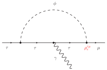
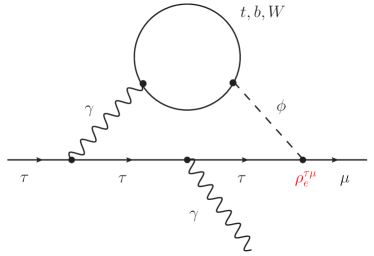
Figure 2: Most important contributions to $\tau\to\mu\gamma$ in the 2HDM. Here $\phi=h,H,A$. To the left, 1-loop diagrams with neutral Higgs bosons and charged leptons in the loop. To the right, 2-loop Barr-Zee diagrams with an internal photon and a third generation quark or a $W$-boson. The LFV vertex proportional to $\rho_{e}^{\tau\mu}$ is explicitly indicated.

The $\tau\to\mu\gamma$ radiative decay is induced by the dipole operator defined by Eqs. (16) and (17). It proves convenient to define the form factors $A_{L}$ and $A_{R}$ as

$$\left(L_{e\gamma}\right)_{\tau\mu}=\frac{e\,m_{\tau}v}{2}\,A_{R}^{\tau\mu}\quad,\quad\left(L_{e\gamma}\right)_{\mu\tau}^{\ast}=\frac{e\,m_{\tau}v}{2}\,A_{L}^{\tau\mu}\,.$$ (37)

Since we assume the matrix $\rho$ to be Hermitian, $|g_{h\tau\mu}|=|g_{h\mu\tau}|$, which implies $|A_{L}|=|A_{R}|\equiv|A|$. We just need to determine the most relevant contributions to the form factor $A$ in the 2HDM.

It is well known that in the 2HDM 2-loop contributions to $\ell_{i}\to\ell_{j}\gamma$ may easily dominate over 1-loop ones [121]. The reason is easy to understand. Dipole transitions require a chirality flip. In a 1–loop diagram with a virtual scalar in the loop, two chirality flips take place in the Yukawa vertices, and therefore one more is required in the fermion propagator, giving a total of three. This largely suppresses the loop amplitude, which explains why 2-loop diagrams with only one chirality flip can be dominant even if one pays the extra loop suppression factor of $1/(16\pi^{2})$. In particular, 2-loop Barr-Zee diagrams [122] can easily dominate if the involved scalar fields have large couplings to the virtual fermions or bosons running in the loops. Taking all these ingredients into account, the authors of Ref. [19] identified three main contributions to $\tau\to\mu\gamma$ in the type-III 2HDM:

• 1-loop diagrams with neutral Higgs bosons and charged leptons in the loop

• 2-loop Barr-Zee diagrams with an internal photon and a third generation quark

• 2-loop Barr-Zee diagrams with an internal photon and a $W$-boson

These contributions were computed in [123] and are shown in Fig. 2. One can write

$$A=\frac{1}{16\pi^{2}}\left(A_{1}+A_{2}^{t,b}+A_{2}^{W}\right)\,,$$ (38)

where the different contributions were computed by [19] and are given explicitly in Appendix A. Armed with these expressions we are ready to explore the HLFV phenomenology of the type-III 2HDM.

4.4 HLFV phenomenology

Following Ref. [9], we show now some phenomenological results on HLFV in the type-III 2HDM. We refer to [31, 34, 42, 46, 47, 53, 56, 124, 72, 76, 78, 87, 89] for additional HLFV phenomenological studies in the 2HDM.

First, we must make an observation about the type-III 2HDM. As already explained, in this version of the 2HDM one can apply rotations in Higgs space that modify the Higgs VEVs. For this reason, the usual ratio of VEVs $\tan\beta$ is not uniquely defined. Given that we are mainly interested in tau flavor violation, we define [120]

$$\tan\beta_{\tau}=\frac{-\rho_{e}^{\tau\tau}}{\sqrt{2}m_{\tau}/v}\,.$$ (39)

We note that $\tan\beta_{\tau}$ is the physical ratio between the tau Yukawa coupling and $\sqrt{2}m_{\tau}/v$, which would correspond to the usual $\tan\beta$ in the Type-II 2HDM.

Let us now discuss our parameter choices. The results presented here are based on a random scan of the parameter space, taking the parameter ranges,

$$200\,\text{GeV}<m_{H}<1000\,\text{GeV}\,,$$

$$400\,\text{GeV}<m_{A}<1000\,\text{GeV}\,,$$

$$-5\,\text{GeV}<m_{H^{\pm}}-m_{A}<5\,\text{GeV}\ ,$$

$$0.7<\sin(\beta-\alpha)<1.0\,,$$

$$0.1<\tan\beta_{\tau}<40\,.$$ (40)

These are based on the following considerations and experimental constraints:

• It proves convenient to use as input the scalar masses, rather than the scalar potential parameters. These should nevertheless be computed to make sure that they never exceed the perturbative limit of $4\pi$. The $\Lambda_{1}$, $\Lambda_{2}$, $\Lambda_{4}$, $\Lambda_{5}$ and $\Lambda_{6}$ parameters can be computed by means of Eqs. (24) - (28). The remaining $\Lambda$ parameters do not have any impact on the observables studied here, but they can be chosen by demanding that the scalar potential is bounded from below [125, 126, 127].

• A small $m_{H^{\pm}}-m_{A}$ mass difference is required by electroweak precision data. In particular, larger values could potentially lead to a $T$ oblique parameter value outside the $1\,\sigma$ range determined by [128], $T\in\left[-0.03,0.19\right]$.

• The lower limit on $\sin(\beta-\alpha)$ is motivated by the fact that the observed Higgs boson has SM-like couplings to fermions and gauge bosons. Lower values of $\sin(\beta-\alpha)$ could potentially induce deviations, see Eqs. (31) and (34), in tension with the experimental results. In our analysis we consider the CMS measurements presented in [129] and require that the signal strengths for $h\to\tau\bar{\tau},b\bar{b},WW^{\ast},ZZ^{\ast}$, defined as $\mu=\left(\sigma\times\text{BR}\right)/\left(\sigma\times\text{BR}\right)_{\text{SM}}$, are within the CMS 1 $\sigma$ ranges [129]. For the determination of the Higgs production cross-section we assume gluon fusion.

• The lower limit on $m_{H^{\pm}}$ is motivated by flavor physics (mainly B physics, see for instance [130]).

Finally, our scan also fixes $m_{h}=125.1$ GeV [131]. In what concerns the Yukawa matrices, and in order to reduce the number of free parameters, we will consider specific textures for the $\rho$ matrices. Inspired by the Cheng-Sher ansatz [132], we express $\rho_{e}$ as

$$\rho_{e}^{ij}=-\kappa_{ij}\,\tan\beta_{\tau}\,\sqrt{\frac{2\,m_{i}\,m_{j}}{v^{2}}}\,.$$ (41)

By construction, $\kappa_{\tau\tau}=1$. However, the other entries of the $\kappa$ matrix are free parameters. In particular, $\kappa_{\tau\mu}=\kappa_{\mu\tau}^{\ast}$ is the relevant parameter giving rise to the $h\to\tau\mu$ and $\tau\to\mu\gamma$ decays. In our random scan we will take $0.1<|\kappa_{\tau\mu}|<3.0$. For the quark $\rho$ matrices we assume the usual Type-II textures

$$\rho_{d}=-\sqrt{2}\,\tan\beta_{\tau}\,\frac{\widehat{\mathcal{M}}_{d}}{v}\quad,\quad\rho_{u}=\sqrt{2}\,\cot\beta_{\tau}\,\frac{K^{\dagger}\,\widehat{\mathcal{M}}_{u}}{v}\,.$$ (42)

This ansatz is particularly convenient since it ensures compatibility with the (already constraining) experimental bounds on the Higgs boson couplings to quarks. Furthermore, it can be regarded as a departure beyond the popular Type-II 2HDM, with the only deviation in the $\tau\mu$ coupling [133]. 

After these preliminaries, we are ready to show some results on $h\to\tau\mu$. Fig. 3 shows $\text{BR}(h\to\tau\mu)$ as a function of $\text{BR}(\tau\to\mu\gamma)$. The vertical lines shown in this figure correspond to the current experimental bound $\text{BR}(\tau\to\mu\gamma)<4.4\times 10^{-8}$ [98] and the expected sensitivity of the Belle-II experiment, of about $\sim 10^{-9}$ [99]. The horizontal line corresponds to the limit $\text{BR}(h\to\tau\mu)<0.0025$, set by the CMS collaboration [95]. As can be seen from this figure, the correlation between these two observables is not exact, and this can be traced back to the different contributions to $\tau\to\mu\gamma$, which might even cancel in some cases. We find that, in general, the dominant contribution to the $\tau\to\mu\gamma$ amplitude comes from 2-loop Barr-Zee diagrams with internal $W$ bosons, although the other contributions typically play a relevant role as well.

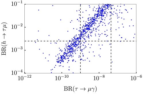
Figure 3: $\text{BR}(h\to\tau\mu)$ as a function of $\text{BR}(\tau\to\mu\gamma)$ in the type-III 2HDM. The parameters are fixed as explained in the text. The vertical lines correspond to the current bound $\text{BR}(\tau\to\mu\gamma)<4.4\times 10^{-8}$ [98] and the expected Belle-II sensitivity, estimated to be $\sim 10^{-9}$ [99]. Finally, the horizontal line indicates the limit by the CMS collaboration $\text{BR}(h\to\tau\mu)<0.0025$ [95].

The main qualitative message that one can extract from Fig. 3 is that the type-III 2HDM can induce $h\to\tau\mu$ rates close to the current bound while being in agreement with all experimental constraints. All LFV observables increase with $\kappa_{\tau\mu}$, and in some regions of the parameter space they can be close to their current experimental limits, explicitly shown in Fig. 3. These regions are characterized by $\tan\beta_{\tau}\gtrsim 2$, $\sin(\beta-\alpha)\sim 0.9$ and $\kappa_{\tau\mu}\gtrsim 0.1$.

Finally, some additional comments are in order. A Higgs doublet with $\mu\tau$ LFV couplings can also address the long-standing muon $g-2$ anomaly. This was studied in relation to the LFV decay $h\to\tau\mu$ in [19, 130, 9, 34, 47, 53, 70, 76], and very recently in [134, 135]. It could also be linked to the popular $b\to s$ [31, 48] or $b\to c$ [42] anomalies observed in B-meson decays or be a crucial ingredient for lepton-flavored electroweak baryogenesis [80]. In fact, the type-III 2HDM with generic Yukawa couplings has a very rich flavor phenomenology, see [130]. The analogous quark flavor violating decay $h\to bs$ was studied in [136]. It is also remarkable that the 2HDM with a BGL symmetry [137, 138, 139] can also lead to large $h\to\tau\mu$ branching ratios, strongly correlated with other flavor observables, as shown in [46]. Here we concentrated on the 2HDM. For HLFV studies in other multi-Higgs doublet models see the interesting works [140, 141, 142, 143].

5 2HDMs, neutrino masses and HLFV

Neutrino flavor oscillations constitute the only existing experimental proof of LFV. Since these are sourced by non-zero neutrino masses and mixings, it is interesting to discuss their possible connection to HLFV [72, 79].

First, one should notice that while the existence of non-zero neutrino masses and mixings implies the violation of lepton flavor, the observation of lepton flavor violating processes does not require neutrinos to be massive. In fact, there are many examples of the latter, the 2HDM being the simplest one. Indeed, in the model presented in Sec. 4.2, the most general 2HDM, neutrino masses are exactly zero but processes such as $\ell_{i}\to\ell_{j}\gamma$ or $h\to\ell_{i}\ell_{j}$ are perfectly possible. Similarly, neutrino masses vanish in the Minimal Supersymmetric Standard Model, but LFV processes are indeed induced if the slepton soft mass contain off-diagonal entries. Other examples are also known, see for instance [144].

There are, however, many neutrino mass models that require the introduction of a second Higgs doublet, and these may potentially lead to an interesting connection between the generation of neutrino masses and HLFV. One of the most popular examples of this link is the Zee model [145], a setup that induces neutrino masses at the 1-loop level.  This model can actually be regarded as an extension of the general 2HDM with the addition of a singly-charged scalar,

$$k\sim\left({\bf 1},{\bf 1},1\right)\,.$$ (43)

If both lepton doublets couple to leptons, as in the type-III 2HDM, the simultaneous presence of the Yukawa term $f\,\bar{\ell}^{c}\,\ell\,k$ and the trilinear scalar potential term $\mu\,\varphi_{1}\,\varphi_{2}\,k^{\dagger}$ breaks lepton number in two units, thus inducing Majorana neutrino masses. Therefore, the model contains all the ingredients to induce neutrino masses and observable HLFV rates. Interestingly, these two consequences of the Zee model are connected in a non-trivial way. Assuming for simplicity $f^{e\mu}=0$, neglecting the electron mass compared to the muon and tau masses, and keeping the term proportional to the muon mass in the (3,3) element to get three massive neutrinos, the neutrino mass matrix is given by [83]

$$\mathcal{M}_{\nu}=A\,s_{2\delta}\,m_{\tau}\,\left(\begin{array}[]{ccc}-2f^{e\tau}\rho_{e}^{\tau e}&-f^{e\tau}\rho_{e}^{\tau\mu}-f^{\mu\tau}\rho_{e}^{\tau e}&\frac{\sqrt{2}s_{\beta_{\tau}}\,m_{\tau}}{v}f^{e\tau}-f^{e\tau}\rho_{e}^{\tau\tau}\\ -f^{e\tau}\rho_{e}^{\tau\mu}-f^{\mu\tau}\rho_{e}^{\tau e}&-2f^{\mu\tau}\rho_{e}^{\tau\mu}&\frac{\sqrt{2}s_{\beta_{\tau}}m_{\tau}}{v}f^{\mu\tau}-f^{\mu\tau}\rho_{e}^{\tau\tau}\\ \frac{\sqrt{2}s_{\beta_{\tau}}\,m_{\tau}}{v}f^{e\tau}-f^{e\tau}\rho_{e}^{\tau\tau}&\frac{\sqrt{2}s_{\beta_{\tau}}m_{\tau}}{v}f^{\mu\tau}-f^{\mu\tau}\rho_{e}^{\tau\tau}&2\frac{m_{\mu}}{m_{\tau}}f^{\mu\tau}\rho_{e}^{\mu\tau}\end{array}\right)\,,$$

where $A$ is a dimensionless combination of model parameters, containing the corresponding loop function, $s_{2\delta}\propto\mu$ quantifies the mixing in the charged scalar sector and we denote $s_{\beta_{\tau}}=\sin\beta_{\tau}$. The $\rho_{e}$ matrix was introduced in Eq. (29). We see that in order to accommodate the measured leptonic mixing angles (see for instance the global fit [147]) both $\rho_{e}^{\tau\mu}$ and $\rho_{e}^{\tau e}$ must be different from zero. Therefore, the Zee model leads to correlations between the leptonic mixing angles and the $h\to\tau\mu$ and $h\to\tau e$ rates. These can be used to set a lower limit on the HLFV rates [83]. For instance, one finds

$$\text{BR}(h\to\tau\mu)\gtrsim 10^{-6}\,\left(10^{-7}\right)$$ (44)

for normal (inverted) neutrino mass ordering. We refer to [83], where a detailed exploration of the parameter space of the Zee model is performed, concluding that the model can accommodate large HLFV rates, even exceeding the current bounds. Similar findings were recently found in [91], where a Zee model supplemented with a flavor-dependent $\rm U(1)$ symmetry was considered.

There are other neutrino mass models including a second Higgs doublet. For instance, in left-right symmetric models [148, 149, 150, 151, 152] one usually introduces a scalar field that is a doublet of both $\rm SU(2)_{L}$ and $\rm SU(2)_{R}$. This bidoublet can be denoted by $\Sigma$ and decomposed as

$$\Sigma=\left(\begin{array}[]{cc}\varphi_{1}^{0}&\varphi_{2}^{+}\\ \varphi_{1}^{-}&\varphi_{2}^{0}\end{array}\right)\,.$$ (45)

The scalar representation $\Sigma$ has two gauge invariant Yukawa couplings to leptons and can be regarded at energies below the $\rm SU(2)_{R}$ breaking scale as a pair of $\rm SU(2)_{L}$ doublets. However, these setups cannot be identified with a type-III 2HDM since the left-right symmetry require the two lepton Yukawa matrices to be Hermitian, thus strongly restricting the allowed parameter space. Furthermore, current limits on quark flavor violation require the second CP-even mass eigenstate, $H$, to have a large mass, $m_{H}\gtrsim 25$ TeV [153], suppressing all HLFV effects. Therefore, the minimal left-right models would have to be enlarged with additional scalar fields in order to be able to provide large HLFV rates [72].

6 Summary and discussion

In this mini-review we have discussed Higgs lepton flavor violating decays, such as $h\to\ell_{i}\ell_{j}$, in the context of the general 2HDM. After motivating this scenario with some model-independent considerations, we have explicitly shown that the 2HDM can indeed allow for large HLFV rates while being in perfect agreement with the experimental constraints at low and high energies. A possible connection to the mechanism behind the generation of neutrino masses is also discussed.

The 2HDM must face many stringent constraints in order to generate large HLFV rates. The first tension comes from existing measurements of the Higgs boson couplings to fermions and gauge bosons, which already place bounds on the parameter that controls the mixing between the two CP-even scalars in the model, $\sin(\beta-\alpha)$. This must necessarily deviate from $1$ in order to allow for non-standard Higgs decays, but not too much in order to be in agreement with the constraints on the Higgs boson couplings. The dipole transitions $\ell_{i}\to\ell_{j}\gamma$ also set very strong limits on the LFV parameters, and these cannot be avoided by any flavor symmetry. However, the associated operators turn out to be suppressed in the 2HDM compared to the operators leading to HLFV, thus increasing the chances to have observable effects of the latter. Taking all these constraints into account, as well as those from electroweak precision data or direct LHC searches, we find that the 2HDM can accommodate HLFV rates arbitrarily close to the current limits, hence making them a very attractive way to search for NP.

The determination of the properties of the recently discovered Higgs boson is among the current priorities for the particle physics community. The increasingly precise measurements of the Higgs couplings and decay rates might eventually reveal a deviation from the SM expectations and hint towards the existence of NP. In particular, the search for HLFV has just started. A positive signal could shed light on questions as central as the flavor puzzle or the fundamental nature of electroweak symmetry breaking.

Appendix A Contributions to $\tau\to\mu\gamma$ in the type-III 2HDM

The most relevant 1- and 2-loop contributions to $\tau\to\mu\gamma$ in the type-III 2HDM were computed in Ref. [19]. Splitting the form factor $A$ as in Eq. (38), these are given by

$$A_{1} =\sqrt{2}\,\sum_{\phi}\frac{g_{\phi\mu\tau}\,g_{\phi\tau\tau}}{m_{\phi}^{2}}\left(\ln\frac{m_{\phi}^{2}}{m_{\tau}^{2}}-\frac{3}{2}\right)\,,$$ (46)

$$A_{2}^{t,b} =6\sum_{\phi,f}g_{\phi\mu\tau}\,g_{\phi ff}\,\frac{Q_{f}^{2}\,\alpha}{\pi\,m_{\tau}\,m_{f}}\,f_{\phi}(r_{f})\,,$$

$$A_{2}^{W} =-\sum_{\phi=h,H}g_{\phi\mu\tau}\,C_{\phi WW}\,\frac{g\,\alpha}{2\,\pi\,m_{\tau}\,m_{W}}\left[3f_{\phi}(r_{W})+\frac{23}{4}g(r_{W})+\frac{3}{4}h(r_{W})+\frac{f_{\phi}(r_{W})-g(r_{W})}{2\,r_{W}}\right]\,.$$

Here $\phi=h,H,A$ and $f$ = $t,b$ and we have defined the ratios

$$r_{f}=\frac{m_{f}^{2}}{m_{\phi}^{2}}\quad\text{and}\quad r_{W}=\frac{m_{W}^{2}}{m_{\phi}^{2}}\,.$$ (47)

In the derivation of these contributions, the charged lepton masses have been neglected whenever possible. The expressions for the $g_{\phi ff^{\prime}}$ and $C_{\phi WW}$ couplings are given in Sec. 4.2. Finally, the loop functions introduced in the previous expressions are given by [123]

$$f_{A}(z)\equiv g(z) =\frac{z}{2}\int_{0}^{1}dx\frac{1}{x(1-x)-z}\ln\frac{x(1-x)}{z}\,,$$ (48)

$$f_{h,H}(z) =\frac{z}{2}\int_{0}^{1}\,dx\,\frac{(1-2x(1-x))}{x(1-x)-z}\ln\frac{x(1-x)}{z}\,,$$ (49)

$$h(z) =-\frac{z}{2}\int_{0}^{1}\frac{dx}{x(1-x)-z}\left[1-\frac{z}{x(1-x)-z}\ln\frac{x(1-x)}{z}\right]\,.$$ (50)

References

- [1] A. Goudelis, O. Lebedev, and J.-h. Park, “Higgs-induced lepton flavor violation,” Phys. Lett. B707 (2012) 369–374, arXiv:1111.1715 [hep-ph].
- [2] G. Blankenburg, J. Ellis, and G. Isidori, “Flavour-Changing Decays of a 125 GeV Higgs-like Particle,” Phys. Lett. B712 (2012) 386–390, arXiv:1202.5704 [hep-ph].
- [3] R. Harnik, J. Kopp, and J. Zupan, “Flavor Violating Higgs Decays,” JHEP 03 (2013) 026, arXiv:1209.1397 [hep-ph].
- [4] A. Dery, A. Efrati, Y. Hochberg, and Y. Nir, “What if ?,” JHEP 05 (2013) 039, arXiv:1302.3229 [hep-ph].
- [5] A. Celis, V. Cirigliano, and E. Passemar, “Lepton flavor violation in the Higgs sector and the role of hadronic -lepton decays,” Phys. Rev. D89 (2014) 013008, arXiv:1309.3564 [hep-ph].
- [6] A. Dery, A. Efrati, Y. Nir, Y. Soreq, and V. Susič, “Model building for flavor changing Higgs couplings,” Phys. Rev. D90 (2014) 115022, arXiv:1408.1371 [hep-ph].
- [7] T. D. Lee, “A Theory of Spontaneous T Violation,” Phys. Rev. D8 (1973) 1226–1239.
- [8] G. C. Branco, “Spontaneous CP Nonconservation and Natural Flavor Conservation: A Minimal Model,” Phys. Rev. D22 (1980) 2901.
- [9] D. Aristizabal Sierra and A. Vicente, “Explaining the CMS Higgs flavor violating decay excess,” Phys. Rev. D90 no. 11, (2014) 115004, arXiv:1409.7690 [hep-ph].
- [10] A. Pilaftsis, “Lepton flavor nonconservation in H0 decays,” Phys. Lett. B285 (1992) 68–74.
- [11] J. L. Diaz-Cruz and J. J. Toscano, “Lepton flavor violating decays of Higgs bosons beyond the standard model,” Phys. Rev. D62 (2000) 116005, arXiv:hep-ph/9910233 [hep-ph].
- [12] M. Sher, “Scalar mediated FCNC at the first muon collider,” Phys. Lett. B487 (2000) 151–154, arXiv:hep-ph/0006159 [hep-ph].
- [13] J. L. Diaz-Cruz, “A More flavored Higgs boson in supersymmetric models,” JHEP 05 (2003) 036, arXiv:hep-ph/0207030 [hep-ph].
- [14] A. Brignole and A. Rossi, “Lepton flavor violating decays of supersymmetric Higgs bosons,” Phys. Lett. B566 (2003) 217–225, arXiv:hep-ph/0304081 [hep-ph].
- [15] J. L. Diaz-Cruz, R. Noriega-Papaqui, and A. Rosado, “Mass matrix ansatz and lepton flavor violation in the THDM-III,” Phys. Rev. D69 (2004) 095002, arXiv:hep-ph/0401194 [hep-ph].
- [16] S. Kanemura, K. Matsuda, T. Ota, T. Shindou, E. Takasugi, and K. Tsumura, “Search for lepton flavor violation in the Higgs boson decay at a linear collider,” Phys. Lett. B599 (2004) 83–91, arXiv:hep-ph/0406316 [hep-ph].
- [17] E. Arganda, A. M. Curiel, M. J. Herrero, and D. Temes, “Lepton flavor violating Higgs boson decays from massive seesaw neutrinos,” Phys. Rev. D71 (2005) 035011, arXiv:hep-ph/0407302 [hep-ph].
- [18] J. K. Parry, “Lepton flavor violating Higgs boson decays, and in the constrained MSSM+NR with large tan beta,” Nucl. Phys. B760 (2007) 38–63, arXiv:hep-ph/0510305 [hep-ph].
- [19] S. Davidson and G. J. Grenier, “Lepton flavour violating Higgs and tau to mu gamma,” Phys. Rev. D81 (2010) 095016, arXiv:1001.0434 [hep-ph].
- [20] A. Dery, A. Efrati, G. Hiller, Y. Hochberg, and Y. Nir, “Higgs couplings to fermions: 2HDM with MFV,” JHEP 08 (2013) 006, arXiv:1304.6727 [hep-ph].
- [21] J. Kopp and M. Nardecchia, “Flavor and CP violation in Higgs decays,” JHEP 10 (2014) 156, arXiv:1406.5303 [hep-ph].
- [22] J. L. Diaz-Cruz, D. K. Ghosh, and S. Moretti, “Lepton Flavour Violating Heavy Higgs Decays Within the nuMSSM and Their Detection at the LHC,” Phys. Lett. B679 (2009) 376–381, arXiv:0809.5158 [hep-ph].
- [23] P. T. Giang, L. T. Hue, D. T. Huong, and H. N. Long, “Lepton-Flavor Violating Decays of Neutral Higgs to Muon and Tauon in Supersymmetric Economical 3-3-1 Model,” Nucl. Phys. B864 (2012) 85–112, arXiv:1204.2902 [hep-ph].
- [24] A. Arhrib, Y. Cheng, and O. C. W. Kong, “Higgs to mu tau Decay in Supersymmetry without R-parity,” EPL 101 no. 3, (2013) 31003, arXiv:1208.4669 [hep-ph].
- [25] A. Arhrib, Y. Cheng, and O. C. W. Kong, “Comprehensive analysis on lepton flavor violating Higgs boson to decay in supersymmetry without parity,” Phys. Rev. D87 no. 1, (2013) 015025, arXiv:1210.8241 [hep-ph].
- [26] M. Arana-Catania, E. Arganda, and M. J. Herrero, “Non-decoupling SUSY in LFV Higgs decays: a window to new physics at the LHC,” JHEP 09 (2013) 160, arXiv:1304.3371 [hep-ph]. [Erratum: JHEP10,192(2015)].
- [27] A. Falkowski, D. M. Straub, and A. Vicente, “Vector-like leptons: Higgs decays and collider phenomenology,” JHEP 05 (2014) 092, arXiv:1312.5329 [hep-ph].
- [28] E. Arganda, M. J. Herrero, X. Marcano, and C. Weiland, “Imprints of massive inverse seesaw model neutrinos in lepton flavor violating Higgs boson decays,” Phys. Rev. D91 no. 1, (2015) 015001, arXiv:1405.4300 [hep-ph].
- [29] CMS Collaboration, V. Khachatryan et al., “Search for Lepton-Flavour-Violating Decays of the Higgs Boson,” Phys. Lett. B749 (2015) 337–362, arXiv:1502.07400 [hep-ex].
- [30] J. Heeck, M. Holthausen, W. Rodejohann, and Y. Shimizu, “Higgs in Abelian and non-Abelian flavor symmetry models,” Nucl. Phys. B896 (2015) 281–310, arXiv:1412.3671 [hep-ph].
- [31] A. Crivellin, G. D’Ambrosio, and J. Heeck, “Explaining , and in a two-Higgs-doublet model with gauged ,” Phys. Rev. Lett. 114 (2015) 151801, arXiv:1501.00993 [hep-ph].
- [32] L. de Lima, C. S. Machado, R. D. Matheus, and L. A. F. do Prado, “Higgs Flavor Violation as a Signal to Discriminate Models,” JHEP 11 (2015) 074, arXiv:1501.06923 [hep-ph].
- [33] I. Doršner, S. Fajfer, A. Greljo, J. F. Kamenik, N. Košnik, and I. Nišandžic, “New Physics Models Facing Lepton Flavor Violating Higgs Decays at the Percent Level,” JHEP 06 (2015) 108, arXiv:1502.07784 [hep-ph].
- [34] Y. Omura, E. Senaha, and K. Tobe, “Lepton-flavor-violating Higgs decay and muon anomalous magnetic moment in a general two Higgs doublet model,” JHEP 05 (2015) 028, arXiv:1502.07824 [hep-ph].
- [35] A. Vicente, “Lepton flavor violation beyond the MSSM,” Adv. High Energy Phys. 2015 (2015) 686572, arXiv:1503.08622 [hep-ph].
- [36] D. Das and A. Kundu, “Two hidden scalars around 125 GeV and ,” Phys. Rev. D92 no. 1, (2015) 015009, arXiv:1504.01125 [hep-ph].
- [37] C.-X. Yue, C. Pang, and Y.-C. Guo, “Lepton flavor violating Higgs couplings and single production of the Higgs boson via e collision,” J. Phys. G42 (2015) 075003, arXiv:1505.02209 [hep-ph].
- [38] B. Bhattacherjee, S. Chakraborty, and S. Mukherjee, “Lepton flavour violating decay of 125 GeV Higgs boson to channel and excess in ,” Mod. Phys. Lett. A31 no. 30, (2016) 1650174, arXiv:1505.02688 [hep-ph].
- [39] T. Kobayashi, Y. Omura, F. Takayama, and D. Yasuhara, “Study of lepton flavor violation in flavor symmetric models for lepton sector,” JHEP 10 (2015) 042, arXiv:1505.07636 [hep-ph].
- [40] Y.-n. Mao and S.-h. Zhu, “Higgs boson-- coupling at high and low energy colliders,” Phys. Rev. D93 no. 3, (2016) 035014, arXiv:1505.07668 [hep-ph].
- [41] X.-G. He, J. Tandean, and Y.-J. Zheng, “Higgs decay with minimal flavor violation,” JHEP 09 (2015) 093, arXiv:1507.02673 [hep-ph].
- [42] A. Crivellin, J. Heeck, and P. Stoffer, “A perturbed lepton-specific two-Higgs-doublet model facing experimental hints for physics beyond the Standard Model,” Phys. Rev. Lett. 116 no. 8, (2016) 081801, arXiv:1507.07567 [hep-ph].
- [43] W. Altmannshofer, S. Gori, A. L. Kagan, L. Silvestrini, and J. Zupan, “Uncovering Mass Generation Through Higgs Flavor Violation,” Phys. Rev. D93 no. 3, (2016) 031301, arXiv:1507.07927 [hep-ph].
- [44] K. Cheung, W.-Y. Keung, and P.-Y. Tseng, “Leptoquark induced rare decay amplitudes and ,” Phys. Rev. D93 no. 1, (2016) 015010, arXiv:1508.01897 [hep-ph].
- [45] E. Arganda, M. J. Herrero, X. Marcano, and C. Weiland, “Enhancement of the lepton flavor violating Higgs boson decay rates from SUSY loops in the inverse seesaw model,” Phys. Rev. D93 no. 5, (2016) 055010, arXiv:1508.04623 [hep-ph].
- [46] F. J. Botella, G. C. Branco, M. Nebot, and M. N. Rebelo, “Flavour Changing Higgs Couplings in a Class of Two Higgs Doublet Models,” Eur. Phys. J. C76 no. 3, (2016) 161, arXiv:1508.05101 [hep-ph].
- [47] X. Liu, L. Bian, X.-Q. Li, and J. Shu, “Type-III two Higgs doublet model plus a pseudoscalar confronted with , muon and dark matter,” Nucl. Phys. B909 (2016) 507–524, arXiv:1508.05716 [hep-ph].
- [48] W. Huang and Y.-L. Tang, “Flavor anomalies at the LHC and the R-parity violating supersymmetric model extended with vectorlike particles,” Phys. Rev. D92 no. 9, (2015) 094015, arXiv:1509.08599 [hep-ph].
- [49] S. Baek and K. Nishiwaki, “Leptoquark explanation of and muon ,” Phys. Rev. D93 no. 1, (2016) 015002, arXiv:1509.07410 [hep-ph].
- [50] S. Baek and Z.-F. Kang, “Naturally Large Radiative Lepton Flavor Violating Higgs Decay Mediated by Lepton-flavored Dark Matter,” JHEP 03 (2016) 106, arXiv:1510.00100 [hep-ph].
- [51] E. Arganda, M. J. Herrero, R. Morales, and A. Szynkman, “Analysis of the decays induced from SUSY loops within the Mass Insertion Approximation,” JHEP 03 (2016) 055, arXiv:1510.04685 [hep-ph].
- [52] D. Aloni, Y. Nir, and E. Stamou, “Large BR() in the MSSM?,” JHEP 04 (2016) 162, arXiv:1511.00979 [hep-ph].
- [53] R. Benbrik, C.-H. Chen, and T. Nomura, “, , in generic two-Higgs-doublet models,” Phys. Rev. D93 no. 9, (2016) 095004, arXiv:1511.08544 [hep-ph].
- [54] H.-B. Zhang, T.-F. Feng, S.-M. Zhao, Y.-L. Yan, and F. Sun, “125 GeV Higgs decay with lepton flavor violation in the SSM,” Chin. Phys. C41 no. 4, (2017) 043106, arXiv:1511.08979 [hep-ph].
- [55] L. T. Hue, H. N. Long, T. T. Thuc, and T. Phong Nguyen, “Lepton flavor violating decays of Standard-Model-like Higgs in 3-3-1 model with neutral lepton,” Nucl. Phys. B907 (2016) 37–76, arXiv:1512.03266 [hep-ph].
- [56] N. Bizot, S. Davidson, M. Frigerio, and J. L. Kneur, “Two Higgs doublets to explain the excesses and ,” JHEP 03 (2016) 073, arXiv:1512.08508 [hep-ph].
- [57] M. Buschmann, J. Kopp, J. Liu, and X.-P. Wang, “New Signatures of Flavor Violating Higgs Couplings,” JHEP 06 (2016) 149, arXiv:1601.02616 [hep-ph].
- [58] X.-F. Han, L. Wang, and J. M. Yang, “An extension of two-Higgs-doublet model and the excesses of 750 GeV diphoton, muon g-2 and ,” Phys. Lett. B757 (2016) 537–547, arXiv:1601.04954 [hep-ph].
- [59] C.-F. Chang, C.-H. V. Chang, C. S. Nugroho, and T.-C. Yuan, “Lepton Flavor Violating Decays of Neutral Higgses in Extended Mirror Fermion Model,” Nucl. Phys. B910 (2016) 293–308, arXiv:1602.00680 [hep-ph].
- [60] H. Bélusca-Maïto and A. Falkowski, “On the exotic Higgs decays in effective field theory,” Eur. Phys. J. C76 no. 9, (2016) 514, arXiv:1602.02645 [hep-ph].
- [61] C.-H. Chen and T. Nomura, “Bounds on LFV Higgs decays in a vector-like lepton model and searching for doubly charged leptons at the LHC,” Eur. Phys. J. C76 no. 6, (2016) 353, arXiv:1602.07519 [hep-ph].
- [62] C. Alvarado, R. M. Capdevilla, A. Delgado, and A. Martin, “Minimal models of loop-induced lepton flavor violation in Higgs boson decays,” Phys. Rev. D94 no. 7, (2016) 075010, arXiv:1602.08506 [hep-ph].
- [63] S. Banerjee, B. Bhattacherjee, M. Mitra, and M. Spannowsky, “The Lepton Flavour Violating Higgs Decays at the HL-LHC and the ILC,” JHEP 07 (2016) 059, arXiv:1603.05952 [hep-ph].
- [64] A. Hayreter, X.-G. He, and G. Valencia, “CP violation in and LFV ,” Phys. Lett. B760 (2016) 175–177, arXiv:1603.06326 [hep-ph].
- [65] K. Huitu, V. Keus, N. Koivunen, and O. Lebedev, “Higgs-flavon mixing and ,” JHEP 05 (2016) 026, arXiv:1603.06614 [hep-ph].
- [66] I. Chakraborty, A. Datta, and A. Kundu, “Lepton flavor violating Higgs boson decay at the ILC,” J. Phys. G43 no. 12, (2016) 125001, arXiv:1603.06681 [hep-ph].
- [67] A. Lami and P. Roig, “ in the simplest little Higgs model,” Phys. Rev. D94 no. 5, (2016) 056001, arXiv:1603.09663 [hep-ph].
- [68] T. T. Thuc, L. T. Hue, H. N. Long, and T. P. Nguyen, “Lepton flavor violating decay of SM-like Higgs boson in a radiative neutrino mass model,” Phys. Rev. D93 no. 11, (2016) 115026, arXiv:1604.03285 [hep-ph].
- [69] S. Baek, T. Nomura, and H. Okada, “An explanation of one-loop induced decay,” Phys. Lett. B759 (2016) 91–98, arXiv:1604.03738 [hep-ph].
- [70] W. Altmannshofer, M. Carena, and A. Crivellin, “ theory of Higgs flavor violation and ,” Phys. Rev. D94 no. 9, (2016) 095026, arXiv:1604.08221 [hep-ph].
- [71] S. Baek and J. Tandean, “Flavor-Changing Higgs Decays in Grand Unification with Minimal Flavor Violation,” Eur. Phys. J. C76 no. 12, (2016) 673, arXiv:1604.08935 [hep-ph].
- [72] J. Herrero-Garcia, N. Rius, and A. Santamaria, “Higgs lepton flavour violation: UV completions and connection to neutrino masses,” JHEP 11 (2016) 084, arXiv:1605.06091 [hep-ph].
- [73] K. H. Phan, H. T. Hung, and L. T. Hue, “One-loop contributions to neutral Higgs decay ,” PTEP 2016 no. 11, (2016) 113B03, arXiv:1605.07164 [hep-ph].
- [74] A. Hammad, S. Khalil, and C. S. Un, “Large BR in Supersymmetric Models,” Phys. Rev. D95 no. 5, (2017) 055028, arXiv:1605.07567 [hep-ph].
- [75] S. V. Demidov and I. V. Sobolev, “Lepton flavor-violating decays of the Higgs boson from sgoldstino mixing,” JHEP 08 (2016) 030, arXiv:1605.08220 [hep-ph].
- [76] L. Wang, S. Yang, and X.-F. Han, “ and muon g-2 in the alignment limit of two-Higgs-doublet model,” Nucl. Phys. B919 (2017) 123–141, arXiv:1606.04408 [hep-ph].
- [77] A. Di Iura, J. Herrero-Garcia, and D. Meloni, “Phenomenology of SU(5) low-energy realizations: the diphoton excess and Higgs flavor violation,” Nucl. Phys. B911 (2016) 388–424, arXiv:1606.08785 [hep-ph].
- [78] K. Tobe, “Michel parameters for decays in a general two Higgs doublet model with flavor violation,” JHEP 10 (2016) 114, arXiv:1607.04447 [hep-ph].
- [79] M. Aoki, S. Kanemura, K. Sakurai, and H. Sugiyama, “Testing neutrino mass generation mechanisms from the lepton flavor violating decay of the Higgs boson,” Phys. Lett. B763 (2016) 352–357, arXiv:1607.08548 [hep-ph].
- [80] H.-K. Guo, Y.-Y. Li, T. Liu, M. Ramsey-Musolf, and J. Shu, “Lepton-Flavored Electroweak Baryogenesis,” Phys. Rev. D96 no. 11, (2017) 115034, arXiv:1609.09849 [hep-ph].
- [81] D. Choudhury, A. Kundu, S. Nandi, and S. K. Patra, “Unified resolution of the and anomalies and the lepton flavor violating decay ,” Phys. Rev. D95 no. 3, (2017) 035021, arXiv:1612.03517 [hep-ph].
- [82] E. Arganda, M. J. Herrero, X. Marcano, R. Morales, and A. Szynkman, “Effective lepton flavor violating vertex from right-handed neutrinos within the mass insertion approximation,” Phys. Rev. D95 no. 9, (2017) 095029, arXiv:1612.09290 [hep-ph].
- [83] J. Herrero-García, T. Ohlsson, S. Riad, and J. Wirén, “Full parameter scan of the Zee model: exploring Higgs lepton flavor violation,” JHEP 04 (2017) 130, arXiv:1701.05345 [hep-ph].
- [84] N. H. Thao, L. T. Hue, H. T. Hung, and N. T. Xuan, “Lepton flavor violating Higgs boson decays in seesaw models: new discussions,” Nucl. Phys. B921 (2017) 159–180, arXiv:1703.00896 [hep-ph].
- [85] S. Chamorro-Solano, A. Moyotl, and M. A. Pérez, “Lepton flavor changing Higgs Boson decays in a Two Higgs Doublet Model with a fourth generation of fermions,” J. Phys. G45 no. 7, (2018) 075003, arXiv:1707.00100 [hep-ph].
- [86] I. Chakraborty, S. Mondal, and B. Mukhopadhyaya, “Lepton flavor violating Higgs boson decay at colliders,” Phys. Rev. D96 no. 11, (2017) 115020, arXiv:1709.08112 [hep-ph].
- [87] Q. Qin, Q. Li, C.-D. Lü, F.-S. Yu, and S.-H. Zhou, “Charged lepton flavor violating Higgs decays at future colliders,” Eur. Phys. J. C78 no. 10, (2018) 835, arXiv:1711.07243 [hep-ph].
- [88] T. P. Nguyen, T. T. Le, T. T. Hong, and L. T. Hue, “Decay of standard model-like Higgs boson in a 3-3-1 model with inverse seesaw neutrino masses,” Phys. Rev. D97 no. 7, (2018) 073003, arXiv:1802.00429 [hep-ph].
- [89] K. S. Babu and S. Jana, “Enhanced Di-Higgs Production in the Two Higgs Doublet Model,” JHEP 02 (2019) 193, arXiv:1812.11943 [hep-ph].
- [90] W.-S. Hou, R. Jain, C. Kao, M. Kohda, B. McCoy, and A. Soni, “Flavor Changing Heavy Higgs Interactions with Leptons at Hadron Colliders,” Phys. Lett. B795 (2019) 371–378, arXiv:1901.10498 [hep-ph].
- [91] T. Nomura and K. Yagyu, “Zee Model with Flavor Dependent Global Symmetry,” arXiv:1905.11568 [hep-ph].
- [92] ATLAS Collaboration, “Search for the decays of the Higgs boson and in collisions at = 13 TeV with the ATLAS detector,” ATLAS-CONF-2019-037 (2019) .
- [93] CMS Collaboration, V. Khachatryan et al., “Search for lepton flavour violating decays of the Higgs boson to and in proton–proton collisions at 8 TeV,” Phys. Lett. B763 (2016) 472–500, arXiv:1607.03561 [hep-ex].
- [94] ATLAS Collaboration, G. Aad et al., “Searches for lepton-flavour-violating decays of the Higgs boson in TeV pp collisions with the ATLAS detector,” arXiv:1907.06131 [hep-ex].
- [95] CMS Collaboration, A. M. Sirunyan et al., “Search for lepton flavour violating decays of the Higgs boson to and e in proton-proton collisions at 13 TeV,” JHEP 06 (2018) 001, arXiv:1712.07173 [hep-ex].
- [96] MEG Collaboration, A. M. Baldini et al., “Search for the lepton flavour violating decay with the full dataset of the MEG experiment,” Eur. Phys. J. C76 no. 8, (2016) 434, arXiv:1605.05081 [hep-ex].
- [97] A. M. Baldini et al., “MEG Upgrade Proposal,” arXiv:1301.7225 [physics.ins-det].
- [98] BaBar Collaboration, B. Aubert et al., “Searches for Lepton Flavor Violation in the Decays and ,” Phys. Rev. Lett. 104 (2010) 021802, arXiv:0908.2381 [hep-ex].
- [99] T. Aushev et al., “Physics at Super B Factory,” arXiv:1002.5012 [hep-ex].
- [100] SINDRUM Collaboration, U. Bellgardt et al., “Search for the Decay ,” Nucl. Phys. B299 (1988) 1–6.
- [101] A. Blondel et al., “Research Proposal for an Experiment to Search for the Decay ,” arXiv:1301.6113 [physics.ins-det].
- [102] K. Hayasaka et al., “Search for Lepton Flavor Violating Tau Decays into Three Leptons with 719 Million Produced Tau+Tau- Pairs,” Phys. Lett. B687 (2010) 139–143, arXiv:1001.3221 [hep-ex].
- [103] SINDRUM II Collaboration, C. Dohmen et al., “Test of lepton flavor conservation in conversion on titanium,” Phys. Lett. B317 (1993) 631–636.
- [104] The PRIME working group Collaboration, “Search for the conversion process at an ultimate sensitivity of the order of with prism.” Unpublished; loi to j-parc 50-gev ps, loi-25, http://www-ps.kek.jp/jhf-np/LOIlist/pdf/L25.pdf.
- [105] SINDRUM II Collaboration, W. H. Bertl et al., “A Search for muon to electron conversion in muonic gold,” Eur. Phys. J. C47 (2006) 337–346.
- [106] Mu2e Collaboration, G. Pezzullo, “The Mu2e experiment at Fermilab: a search for lepton flavor violation,” Nucl. Part. Phys. Proc. 285-286 (2017) 3–7, arXiv:1705.06461 [hep-ex].
- [107] DeeMe Collaboration, H. Natori, “DeeMe experiment - An experimental search for a mu-e conversion reaction at J-PARC MLF,” Nucl. Phys. Proc. Suppl. 248-250 (2014) 52–57.
- [108] L. Calibbi and G. Signorelli, “Charged Lepton Flavour Violation: An Experimental and Theoretical Introduction,” Riv. Nuovo Cim. 41 no. 2, (2018) 71–174, arXiv:1709.00294 [hep-ph].
- [109] S. T. Petcov, “The Processes , , in the Weinberg-Salam Model with Neutrino Mixing,” Sov. J. Nucl. Phys. 25 (1977) 340. [Erratum: Yad. Fiz.25,1336(1977)].
- [110] B. Grzadkowski, M. Iskrzynski, M. Misiak, and J. Rosiek, “Dimension-Six Terms in the Standard Model Lagrangian,” JHEP 10 (2010) 085, arXiv:1008.4884 [hep-ph].
- [111] A. Celis, J. Fuentes-Martin, A. Vicente, and J. Virto, “DsixTools: The Standard Model Effective Field Theory Toolkit,” Eur. Phys. J. C77 no. 6, (2017) 405, arXiv:1704.04504 [hep-ph].
- [112] E. E. Jenkins, A. V. Manohar, and P. Stoffer, “Low-Energy Effective Field Theory below the Electroweak Scale: Operators and Matching,” JHEP 03 (2018) 016, arXiv:1709.04486 [hep-ph].
- [113] R. Alonso, E. E. Jenkins, A. V. Manohar, and M. Trott, “Renormalization Group Evolution of the Standard Model Dimension Six Operators III: Gauge Coupling Dependence and Phenomenology,” JHEP 04 (2014) 159, arXiv:1312.2014 [hep-ph].
- [114] S. L. Glashow and S. Weinberg, “Natural Conservation Laws for Neutral Currents,” Phys. Rev. D15 (1977) 1958.
- [115] E. A. Paschos, “Diagonal Neutral Currents,” Phys. Rev. D15 (1977) 1966.
- [116] G. C. Branco, P. M. Ferreira, L. Lavoura, M. N. Rebelo, M. Sher, and J. P. Silva, “Theory and phenomenology of two-Higgs-doublet models,” Phys. Rept. 516 (2012) 1–102, arXiv:1106.0034 [hep-ph].
- [117] H. Georgi and D. V. Nanopoulos, “Suppression of Flavor Changing Effects From Neutral Spinless Meson Exchange in Gauge Theories,” Phys. Lett. 82B (1979) 95–96.
- [118] J. F. Donoghue and L. F. Li, “Properties of Charged Higgs Bosons,” Phys. Rev. D19 (1979) 945.
- [119] F. J. Botella and J. P. Silva, “Jarlskog - like invariants for theories with scalars and fermions,” Phys. Rev. D51 (1995) 3870–3875, arXiv:hep-ph/9411288 [hep-ph].
- [120] S. Davidson and H. E. Haber, “Basis-independent methods for the two-Higgs-doublet model,” Phys. Rev. D72 (2005) 035004, arXiv:hep-ph/0504050 [hep-ph]. [Erratum: Phys. Rev.D72,099902(2005)].
- [121] J. D. Bjorken, K. D. Lane, and S. Weinberg, “The Decay in Models with Neutral Heavy Leptons,” Phys. Rev. D16 (1977) 1474.
- [122] S. M. Barr and A. Zee, “Electric Dipole Moment of the Electron and of the Neutron,” Phys. Rev. Lett. 65 (1990) 21–24. [Erratum: Phys. Rev. Lett.65,2920(1990)].
- [123] D. Chang, W. S. Hou, and W.-Y. Keung, “Two loop contributions of flavor changing neutral Higgs bosons to ,” Phys. Rev. D48 (1993) 217–224, arXiv:hep-ph/9302267 [hep-ph].
- [124] M. Sher and K. Thrasher, “Flavor Changing Leptonic Decays of Heavy Higgs Bosons,” Phys. Rev. D93 no. 5, (2016) 055021, arXiv:1601.03973 [hep-ph].
- [125] I. P. Ivanov, “Minkowski space structure of the Higgs potential in 2HDM,” Phys. Rev. D75 (2007) 035001, arXiv:hep-ph/0609018 [hep-ph]. [Erratum: Phys. Rev.D76,039902(2007)].
- [126] I. P. Ivanov, “Minkowski space structure of the Higgs potential in 2HDM. II. Minima, symmetries, and topology,” Phys. Rev. D77 (2008) 015017, arXiv:0710.3490 [hep-ph].
- [127] P. M. Ferreira and D. R. T. Jones, “Bounds on scalar masses in two Higgs doublet models,” JHEP 08 (2009) 069, arXiv:0903.2856 [hep-ph].
- [128] M. Baak, M. Goebel, J. Haller, A. Hoecker, D. Kennedy, R. Kogler, K. Moenig, M. Schott, and J. Stelzer, “The Electroweak Fit of the Standard Model after the Discovery of a New Boson at the LHC,” Eur. Phys. J. C72 (2012) 2205, arXiv:1209.2716 [hep-ph].
- [129] CMS Collaboration, “Precise determination of the mass of the Higgs boson and studies of the compatibility of its couplings with the standard model,” Tech. Rep. CMS-PAS-HIG-14-009, CERN, Geneva, 2014. https://cds.cern.ch/record/1728249.
- [130] A. Crivellin, A. Kokulu, and C. Greub, “Flavor-phenomenology of two-Higgs-doublet models with generic Yukawa structure,” Phys. Rev. D87 no. 9, (2013) 094031, arXiv:1303.5877 [hep-ph].
- [131] Particle Data Group Collaboration, M. Tanabashi et al., “Review of Particle Physics,” Phys. Rev. D98 no. 3, (2018) 030001.
- [132] T. P. Cheng and M. Sher, “Mass Matrix Ansatz and Flavor Nonconservation in Models with Multiple Higgs Doublets,” Phys. Rev. D35 (1987) 3484.
- [133] S. Kanemura, T. Ota, and K. Tsumura, “Lepton flavor violation in Higgs boson decays under the rare tau decay results,” Phys. Rev. D73 (2006) 016006, arXiv:hep-ph/0505191 [hep-ph].
- [134] S. Iguro, Y. Omura, and M. Takeuchi, “Testing the 2HDM explanation of the muon g-2 anomaly at the LHC,” arXiv:1907.09845 [hep-ph].
- [135] L. Wang and Y. Zhang, “A --philic Higgs doublet confronted with the muon g-2, decays and LHC data,” arXiv:1908.03755 [hep-ph].
- [136] A. Crivellin, J. Heeck, and D. Müller, “Large in generic two-Higgs-doublet models,” Phys. Rev. D97 no. 3, (2018) 035008, arXiv:1710.04663 [hep-ph].
- [137] G. C. Branco, W. Grimus, and L. Lavoura, “Relating the scalar flavor changing neutral couplings to the CKM matrix,” Phys. Lett. B380 (1996) 119–126, arXiv:hep-ph/9601383 [hep-ph].
- [138] F. J. Botella, G. C. Branco, and M. N. Rebelo, “Minimal Flavour Violation and Multi-Higgs Models,” Phys. Lett. B687 (2010) 194–200, arXiv:0911.1753 [hep-ph].
- [139] F. J. Botella, G. C. Branco, M. Nebot, and M. N. Rebelo, “Two-Higgs Leptonic Minimal Flavour Violation,” JHEP 10 (2011) 037, arXiv:1102.0520 [hep-ph].
- [140] G. Bhattacharyya, P. Leser, and H. Päs, “Exotic Higgs boson decay modes as a harbinger of flavor symmetry,” Phys. Rev. D83 (2011) 011701, arXiv:1006.5597 [hep-ph].
- [141] G. Bhattacharyya, P. Leser, and H. Päs, “Novel signatures of the Higgs sector from flavor symmetry,” Phys. Rev. D86 (2012) 036009, arXiv:1206.4202 [hep-ph].
- [142] M. A. Arroyo-Ureña, J. L. Diaz-Cruz, E. Díaz, and J. A. Orduz-Ducuara, “Flavor violating Higgs signals in the Texturized Two-Higgs Doublet Model (THDM-Tx),” Chin. Phys. C40 no. 12, (2016) 123103, arXiv:1306.2343 [hep-ph].
- [143] M. D. Campos, A. E. Cárcamo Hernández, H. Päs, and E. Schumacher, “Higgs as an indication for flavor symmetry,” Phys. Rev. D91 no. 11, (2015) 116011, arXiv:1408.1652 [hep-ph].
- [144] J. Bernabeu, A. Santamaria, J. Vidal, A. Mendez, and J. W. F. Valle, “Lepton Flavor Nonconservation at High-Energies in a Superstring Inspired Standard Model,” Phys. Lett. B187 (1987) 303–308.
- [145] A. Zee, “A Theory of Lepton Number Violation, Neutrino Majorana Mass, and Oscillation,” Phys. Lett. 93B (1980) 389. [Erratum: Phys. Lett.95B,461(1980)].
- [146] Y. Cai, J. Herrero-García, M. A. Schmidt, A. Vicente, and R. R. Volkas, “From the trees to the forest: a review of radiative neutrino mass models,” Front.in Phys. 5 (2017) 63, arXiv:1706.08524 [hep-ph].
- [147] P. F. de Salas, D. V. Forero, C. A. Ternes, M. Tortola, and J. W. F. Valle, “Status of neutrino oscillations 2018: 3 hint for normal mass ordering and improved CP sensitivity,” Phys. Lett. B782 (2018) 633–640, arXiv:1708.01186 [hep-ph].
- [148] J. C. Pati and A. Salam, “Lepton Number as the Fourth Color,” Phys. Rev. D10 (1974) 275–289. [Erratum: Phys. Rev.D11,703(1975)].
- [149] R. N. Mohapatra and J. C. Pati, “A Natural Left-Right Symmetry,” Phys. Rev. D11 (1975) 2558.
- [150] G. Senjanovic and R. N. Mohapatra, “Exact Left-Right Symmetry and Spontaneous Violation of Parity,” Phys. Rev. D12 (1975) 1502.
- [151] R. N. Mohapatra and G. Senjanovic, “Neutrino Mass and Spontaneous Parity Nonconservation,” Phys. Rev. Lett. 44 (1980) 912. [,231(1979)].
- [152] R. N. Mohapatra and G. Senjanovic, “Neutrino Masses and Mixings in Gauge Models with Spontaneous Parity Violation,” Phys. Rev. D23 (1981) 165.
- [153] Y. Zhang, H. An, X. Ji, and R. N. Mohapatra, “General CP Violation in Minimal Left-Right Symmetric Model and Constraints on the Right-Handed Scale,” Nucl. Phys. B802 (2008) 247–279, arXiv:0712.4218 [hep-ph].