Asymmetric Non-local Neural Networks for Semantic Segmentation

Abstract

The non-local module works as a particularly useful technique for semantic segmentation while criticized for its prohibitive computation and GPU memory occupation. In this paper, we present Asymmetric Non-local Neural Network to semantic segmentation, which has two prominent components: Asymmetric Pyramid Non-local Block (APNB) and Asymmetric Fusion Non-local Block (AFNB). APNB leverages a pyramid sampling module into the non-local block to largely reduce the computation and memory consumption without sacrificing the performance. AFNB is adapted from APNB to fuse the features of different levels under a sufficient consideration of long range dependencies and thus considerably improves the performance. Extensive experiments on semantic segmentation benchmarks demonstrate the effectiveness and efficiency of our work. In particular, we report the state-of-the-art performance of 81.3 mIoU on the Cityscapes test set. For a $256\times 128$ input, APNB is around 6 times faster than a non-local block on GPU while 28 times smaller in GPU running memory occupation. Code is available at: https://github.com/MendelXu/ANN.git.

1 Introduction

Semantic segmentation is a long-standing challenging task in computer vision, aiming to predict pixel-wise semantic labels in an image accurately. This task is exceptionally important to tons of real-world applications, such as autonomous driving [27, 28], medical diagnosing [52, 53], etc. In recent years, the developments of deep neural networks encourage the emergence of a series of works [1, 5, 18, 26, 40, 43, 47]. Shelhamer et al. [26] proposed the seminal work called Fully Convolutional Network (FCN), which discarded the fully connected layer to support input of arbitrary sizes. Since then, a lot of works [5, 18] were inspired to manipulate FCN techniques into deep neural networks. Nonetheless, the segmentation accuracy is still far from satisfactory.

Some recent studies [20, 33, 47] indicate that the performance could be improved if making sufficient use of long range dependencies. However, models that solely rely on convolutions exhibit limited ability in capturing these long range dependencies. A possible reason is the receptive field of a single convolutional layer is inadequate to cover correlated areas. Choosing a big kernel or composing a very deep network is able to enlarge the receptive field. However, such strategies require extensive computation and parameters, thus being very inefficient [44]. Consequently, several works [33, 47] resort to use global operations like non-local means [2] and spatial pyramid pooling [12, 16].

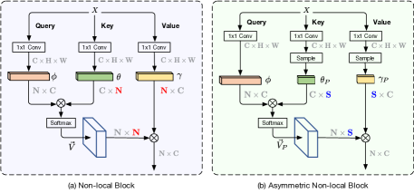
Figure 1: Architecture of a standard non-local block (a) and the asymmetric non-local block (b). $N=H\cdot W$ while $S\ll N$.

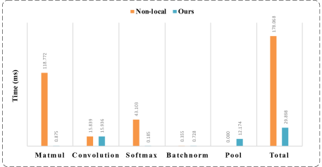
Figure 2: GPU time ( $\geq 1$ ms) comparison of different operations between a generic non-local block and our APNB. The last bin denotes the sum of all the time costs. The size of the inputs for these two blocks is $256\times 128$.

In [33], Wang et al. combined CNNs and traditional non-local means [2] to compose a network module named non-local block in order to leverage features from all locations in an image. This module improves the performance of existing methods [33]. However, the prohibitive computational cost and vast GPU memory occupation hinder its usage in many real applications. The architecture of a common non-local block [33] is depicted in Fig. 1(a). The block first calculates the similarities of all locations between each other, requiring a matrix multiplication of computational complexity $\mathcal{O}(CH^{2}W^{2})$, given an input feature map with size $C\times H\times W$. Then it requires another matrix multiplication of computational complexity $\mathcal{O}(CH^{2}W^{2})$ to gather the influence of all locations to themselves. Concerning the high complexity brought by the matrix multiplications, we are interested in this work if there are efficient ways to solve this without sacrificing the performance.

We notice that as long as the outputs of the key branch and value branch hold the same size, the output size of the non-local block remains unchanged. Considering this, if we could sample only a few representative points from key branch and value branch, it is possible that the time complexity is significantly decreased without sacrificing the performance. This motivation is demonstrated in Fig. 1 when changing a large value ${\color[rgb]{1,0,0}N}$ in the key branch and value branch to a much smaller value ${\color[rgb]{0,0,1}S}$ (From (a) to (b)).

In this paper, we propose a simple yet effective non-local module called Asymmetric Pyramid Non-local Block (APNB) to decrease the computation and GPU memory consumption of the standard non-local module [33] with applications to semantic segmentation. Motivated by the spatial pyramid pooling [12, 16, 47] strategy, we propose to embed a pyramid sampling module into non-local blocks, which could largely reduce the computation overhead of matrix multiplications yet provide substantial semantic feature statistics. This spirit is also related to the sub-sampling tricks [33] (e.g., max pooling). Our experiments suggest that APNB yields much better performance than those sub-sampling tricks with a decent decrease of computations. To better illustrate the boosted efficiency, we compare the GPU times of APNB and a standard non-local block in Fig. 2, averaging the running time of 10 different runs with the same configuration. Our APNB largely reduces the time cost on matrix multiplications, thus being nearly 6 times faster than a non-local block.

Besides, we also adapt APNB to fuse the features of different stages of a deep network, which brings a considerable improvement over the baseline model. We call the adapted block as Asymmetric Fusion Non-local Block (AFNB). AFNB calculates the correlations between every pixel of the low-level and high-level feature maps, yielding a fused feature with long range interactions. Our network is built based on a standard ResNet-FCN model by integrating APNB and AFNB together.

The efficacy of the proposed network is evaluated on Cityscapes [9], ADE20K [50] and PASCAL Context [21], achieving the state-of-the-art performance 81.3%, 45.24% and 52.8%, respectively. In terms of time and space efficiency, APNB is around 6 times faster than a non-local block on a GPU while 28 times smaller in GPU running memory occupation for a $256\times 128$ input.

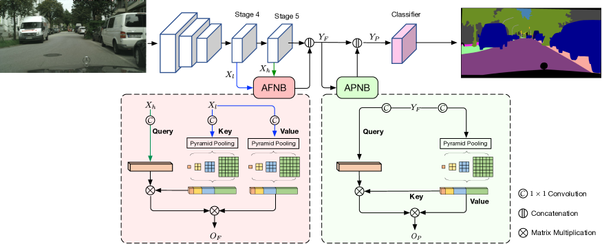
Figure 3: Overview of the proposed Asymmetric Non-local Neural Network. In our implementation, the key branch and the value branch in APNB share the same $1\times 1$ convolution and sampling module, which decreases the number of parameters and computation without sacrificing the performance.

2 Related Work

In this section, we briefly review related works about semantic segmentation or scene parsing. Recent advances focus on exploring the context information and can be roughly categorized into five directions:

Encoder-Decoder. A encoder generally reduces the spatial size of feature maps to enlarge the receptive field. Then the encoded codes are fed to the decoder, which is responsible for recovering the spatial size of the prediction maps. Long et al. [26] and Noh et al. [22] used deconvolutions to perform the decoding pass. Ronneberger et al. [25] introduced skip-connections to bridge the encoding features to their corresponding decoding features, which could enrich the segmentation output with more details. Zhang et al. [43] introduced a context encoding module to predict semantic category importance and selectively strengthen or weaken class-specific feature maps.

CRF. As a frequently-used operation that could leverage context information in machine learning, Conditional Random Field [15] meets its new opportunity in combining with CNNs for semantic segmentation [4, 5, 6, 49, 31]. CRF-CNN [49] adopted this strategy, making the deep network end-to-end trainable. Chandra et al. [4] and Vemulapalli et al. [31] integrated Gaussian Conditional Random Fields into CNNs and achieved relatively good results.

Different Convolutions. Chen et al. [5, 6] and Yu et al. [40] adapted generic convolutions to dilated ones, making the networks sensitive to global context semantics and thus improves the performance. Peng et al. [24] found large kernel convolutions help relieve the contradiction between classification and localization in segmentation.

Spatial Pyramid Pooling. Inspired by the success of spatial pyramid pooling in object detection [12], Chen et al. [6] replaced the pooling layers with dilated convolutions of different sampling weights and built an Atrous Spatial Pyramid Pooling layer (ASPP) to account for multiple scales explicitly. Chen et al. [8] further combined ASPP and the encoder-decoder architecture to leverage the advantages of both and boost the performance considerably. Drawing inspiration from [16], PSPNet [47] conducted spatial pyramid pooling after a specific layer to embed context features of different scales into the networks. Recently, Yang et al. [36] pointed out the ASPP layer has a restricted receptive field and adapted ASPP to a densely connected version, which helps to overcome such limitation.

Non-local Network. Recently, researchers [20, 33, 47] noticed that skillful leveraging the long range dependencies brings great benefits to semantic segmentation. Wang et al. [33] proposed a non-local block module combining non-local means with deep networks and showcased its efficacy for segmentation.

Different from these works, our network uniquely incorporates pyramid sampling strategies with non-local blocks to capture the semantic statistics of different scales with only a minor budget of computation, while maintaining the excellent performance as the original non-local modules.

3 Asymmetric Non-local Neural Network

In this section, we firstly revisit the definition of non-local block [33] in Sec. 3.1, then detail the proposed Asymmetrical Pyramid Non-local Block (APNB) and Asymmetrical Fusion Non-local Block (AFNB) in Sec. 3.2 and Sec. 3.3, respectively. While APNB aims to decrease the computational overhead of non-local blocks, AFNB improves the learning capacity of non-local blocks thereby improving the segmentation performance.

3.1 Revisiting Non-local Block

A typical non-local block [33] is shown in Fig. 1. Consider an input feature $X\in\mathcal{R}^{C\times H\times W}$, where $C$, $W$, and $H$ indicate the channel number, spatial width and height, respectively. Three $1\times 1$ convolutions $W_{\phi}$, $W_{\theta}$, and $W_{\gamma}$ are used to transform $X$ to different embeddings $\phi\in{R}^{\hat{C}\times H\times W}$, $\theta\in\mathcal{R}^{\hat{C}\times H\times W}$ and $\gamma\in\mathcal{R}^{\hat{C}\times H\times W}$ as

$$\phi=W_{\phi}(\mathcal{X}),~{}~{}\theta=W_{\theta}(\mathcal{X}),~{}~{}\gamma=W_{\gamma}(\mathcal{X}),$$ (1)

where $\hat{C}$ is the channel number of the new embeddings. Next, the three embeddings are flattened to size $\hat{C}\times N$, where $N$ represents the total number of the spatial locations, that is, $N=H\cdot W$. Then, the similarity matrix $V\in\mathcal{R}^{N\times N}$ is calculated by a matrix multiplication as

$$V=\phi^{\mathrm{T}}\times\theta.$$ (2)

Afterward, a normalization is applied to $V$ to get a unified similarity matrix as

$$\vec{V}=f(V).$$ (3)

According to [33], the normalizing function $f$ can take the form from $\mathrm{softmax}$, $\mathrm{rescaling}$, and $\mathrm{none}$. We choose $\mathrm{softmax}$ here, which is equivalent to the self-attention mechanism and proved to work well in many tasks such as machine translation [30] and image generation [44]. For every location in $\gamma$, the output of the attention layer is

$$O=\vec{V}\times\gamma^{\mathrm{T}},$$ (4)

where $O\in\mathcal{R}^{N\times\hat{C}}$. By referring to the design of the non-local block, the final output is given by

$$Y=W_{o}(O^{\mathrm{T}})+X\ \mathrm{or}\ Y=\mathrm{cat}(W_{o}(O^{\mathrm{T}}),X),$$ (5)

where $W_{o}$, also implemented by a $1\times 1$ convolution, acts as a weighting parameter to adjust the importance of the non-local operation w.r.t. missing the original input $X$ and moreover, recovers the channel dimension from $\hat{C}$ to $C$.

3.2 Asymmetric Pyramid Non-local Block

The non-local network is potent to capture the long range dependencies that are crucial for semantic segmentation. However, the non-local operation is very time and memory consuming compared to normal operations in the deep neural network, e.g., convolutions and activation functions.

Motivation and Analysis. By inspecting the general computing flow of a non-local block, one could clearly find that Eq. (2) and Eq. (4) dominate the computation. The time complexities of the two matrix multiplications are both $\mathcal{O}(\hat{C}N^{2})=\mathcal{O}(\hat{C}H^{2}W^{2})$. In semantic segmentation, the output of the network usually has a large resolution to retain detailed semantic features [6, 47]. That means $N$ is large (for example in our training phase, $N=96\times 96=9216$). Hence, the large matrix multiplication is the main cause of the inefficiency of a non-local block (see our statistic in Fig. 2).

A more straightforward pipeline is given as

$$\underbrace{\mathcal{R}^{{N}\times\hat{C}}\times\mathcal{R}^{\hat{C}\times{\color[rgb]{1,0,0}N}}}_{Eq.\eqref{matmul1}}\rightarrow\underbrace{\mathcal{R}^{{N}\times{\color[rgb]{1,0,0}N}}\times\mathcal{R}^{{\color[rgb]{1,0,0}N}\times\hat{C}}}_{Eq.\eqref{matmul2}}\rightarrow\mathcal{R}^{N\times\hat{C}}.$$ (6)

We hold a key yet intuitive observation that by changing ${\color[rgb]{1,0,0}N}$ to another number ${\color[rgb]{0,0,1}S}$ (${\color[rgb]{0,0,1}S}\ll{\color[rgb]{1,0,0}N}$), the output size will remain the same, as

$$\mathcal{R}^{{N}\times\hat{C}}\times\mathcal{R}^{\hat{C}\times{\color[rgb]{0,0,1}S}}\rightarrow\mathcal{R}^{{N}\times{\color[rgb]{0,0,1}S}}\times\mathcal{R}^{{\color[rgb]{0,0,1}S}\times\hat{C}}\rightarrow\mathcal{R}^{N\times\hat{C}}.$$ (7)

Returning to the design of the non-local block, changing ${\color[rgb]{1,0,0}N}$ to a small number ${\color[rgb]{0,0,1}S}$ is equivalent to sampling several representative points from $\theta$ and $\gamma$ instead of feeding all the spatial points, as illustrated in Fig. 1. Consequently, the computational complexity could be considerably decreased.

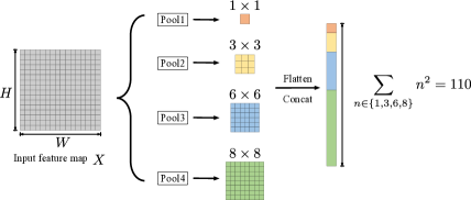
Figure 4: Demonstration of the pyramid max or average sampling process.

Solution. Based on the above observation, we propose to add sampling modules $\mathcal{P}_{\theta}$ and $\mathcal{P}_{\gamma}$ after $\theta$ and $\gamma$ to sample several sparse anchor points denoted as $\theta_{P}\in\mathcal{R}^{\hat{C}\times{\color[rgb]{0,0,1}S}}$ and $\gamma_{P}\in\mathcal{R}^{\hat{C}\times{\color[rgb]{0,0,1}S}}$, where ${\color[rgb]{0,0,1}S}$ is the number of sampled anchor points. Mathematically, this is computed by

$$\theta_{P}=\mathcal{P}_{\theta}(\theta),~{}~{}\gamma_{P}=\mathcal{P}_{\gamma}(\gamma).$$ (8)

The similarity matrix $V_{P}$ between $\phi$ and the anchor points $\theta_{P}$ is thus calculated by

$$V_{P}=\phi^{\mathrm{T}}\times\theta_{P}.$$ (9)

Note that $V_{P}$ is an asymmetric matrix of size $N\times{\color[rgb]{0,0,1}S}$. $V_{P}$ then goes through the same normalizing function as a standard non-local block, giving the unified similarity matrix $\vec{V}_{P}$. And the attention output is acquired by

$$O_{P}=\vec{V}_{P}\times{\gamma_{P}}^{\mathrm{T}},$$ (10)

where the output is in the same size as that of Eq. (4). Following non-local blocks, the final output $Y_{P}$ is given as

$$Y_{P}=\mathrm{cat}(W_{o}({O_{P}}^{\mathrm{T}}),X).$$ (11)

The time complexity of such an asymmetric matrix multiplication is only $\mathcal{O}(\hat{C}NS)$, significantly lower than $\mathcal{O}(\hat{C}N^{2})$ in a standard non-local block. It is ideal that ${\color[rgb]{0,0,1}S}$ should be much smaller than ${\color[rgb]{1,0,0}N}$. However, it is hard to ensure that when ${\color[rgb]{0,0,1}S}$ is small, the performance would not drop too much in the meantime.

As discovered by previous works [16, 47], global and multi-scale representations are useful for categorizing scene semantics. Such representations can be comprehensively carved by Spatial Pyramid Pooling [16], which contains several pooling layers with different output sizes in parallel. In addition to this virtue, spatial pyramid pooling is also parameter-free and very efficient. Therefore, we embed pyramid pooling in the non-local block to enhance the global representations while reducing the computational overhead.

By doing so, we now arrive at the final formulation of Asymmetric Pyramid Non-local Block (APNB), as given in Fig. 3. As can be seen, our APNB derives from the design of a standard non-local block [33]. A vital change is to add a spatial pyramid pooling module after $\theta$ and $\gamma$ respectively to sample representative anchors. This sampling process is clearly depicted in Fig. 4, where several pooling layers are applied after $\theta$ or $\gamma$ and then the four pooling results are flattened and concatenated to serve as the input to the next layer. We denote the spatial pyramid pooling modules as $\mathcal{P}_{\theta}^{n}$ and $\mathcal{P}_{\gamma}^{n}$, where the superscript $n$ means the width (or height) of the output size of the pooling layer (empirically, the width is equal to the height). In our model, we set $n\subseteq\{1,3,6,8\}$. Then the total number of the anchor points is

$$S=110=\sum_{n\in\{1,3,6,8\}}n^{2}.$$ (12)

As a consequence, the complexity of our asymmetric matrix multiplication is only

$$T=\frac{S}{N}$$ (13)

times of the complexity of the non-local matrix multiplication. When $H=128$ and $W=256$, the asymmetrical matrix multiplication saves us $\frac{256\times 128}{110}\approx 298$ times of computation (see the results in Fig. 2). Moreover, the spatial pyramid pooling gives sufficient feature statistics about the global scene semantic cues to remedy the potential performance deterioration caused by the decreased computation. We will analyze this in our experiments.

3.3 Asymmetric Fusion Non-local Block

Fusing features of different levels are helpful to semantic segmentation and object tracking as hinted in [16, 18, 26, 41, 46, 51]. Common fusing operations such as addition/concatenation, are conducted in a pixel-wise and local manner. We provide an alternative that leverages long range dependencies through a non-local block to fuse multi-level features, called Fusion Non-local Block.

A standard non-local block only has one input source while FNB has two: a high-level feature map $X_{h}\in\mathcal{R}^{C_{h}\times N_{h}}$ and a low-level feature map $X_{l}\in\mathcal{R}^{C_{l}\times N_{l}}$. $N_{h}$ and $N_{l}$ are the numbers of spatial locations of $X_{h}$ and $X_{l}$, respectively. $C_{h}$ and $C_{l}$ are the channel numbers of $X_{h}$ and $X_{l}$, respectively. Likewise, $1\times 1$ convolutions $W_{\phi}^{h}$, $W_{\theta}^{l}$ and $W_{\gamma}^{l}$ are used to transform $X_{h}$ and $X_{l}$ to embeddings ${\phi}_{h}\in\mathcal{R}^{\hat{C}\times N_{h}}$, ${\theta}_{l}\in\mathcal{R}^{\hat{C}\times N_{l}}$ and ${\gamma}_{l}\in\mathcal{R}^{\hat{C}\times N_{l}}$ as

$${\phi}_{h}=W_{\phi}^{h}(\mathcal{X}_{h}),\ {\theta}_{l}=W_{\theta}^{l}(\mathcal{X}_{l}),\ {\gamma}_{l}=W_{\gamma}^{l}(\mathcal{X}_{l}).$$ (14)

Then, the similarity matrix $V_{F}\in\mathcal{R}^{N_{h}\times N_{l}}$ between ${\phi}_{h}$ and ${\theta}_{l}$ is computed by a matrix multiplication

$$V_{F}={{\phi}_{h}}^{\mathrm{T}}\times{\theta}_{l}.$$ (15)

We also put a normalization upon $V_{F}$ resulting in a unified similarity matrix $\vec{V}_{F}\in\mathcal{R}^{N_{h}\times N_{l}}$. Afterward, we integrate $\vec{V}_{F}$ with $\gamma_{l}$ through a similar matrix multiplication as Eq. (4) and Eq. (10), written as

$$O_{F}=\vec{V}_{F}\times{\gamma}_{l}^{\mathrm{T}}.$$ (16)

The output $O_{F}\in\mathcal{R}^{N_{h}\times\hat{C}}$ reflects the bonus of $X_{l}$ to $X_{h}$, which are carefully selected from all locations in $X_{l}$. Likewise, $O_{F}$ is fed to a $1\times 1$ convolution to recover the channel number to $C_{h}$. Finally, we have the output as

$$Y_{F}=\mathrm{cat}(W_{o}({O_{F}}^{\mathrm{T}}),X_{h}).$$ (17)

Similar to the adaption of APNB w.r.t. missing the generic non-local block, incorporating spatial pyramid pooling into FNB could derive an efficient Asymmetric Fusion Non-local Block (AFNB), as illustrated in Fig. 3. Inheriting from the advantages of APNB, AFNB is more efficient than FNB without sacrificing the performance.

3.4 Network Architecture

The overall architecture of our network is depicted in Fig. 3. We choose ResNet-101 [13] as our backbone network following the choice of most previous works [38, 47, 48]. We remove the last two down-sampling operations and use the dilation convolutions instead to hold the feature maps from the last two stages $\frac{1}{8}$ of the input image. Concretely, all the feature maps in the last three stages have the same spatial size. According to our experimental trials, we fuse the features of $\mathrm{Stage4}$ and $\mathrm{Stage5}$ using AFNB. The fused features are thereupon concatenated with the feature maps after $\mathrm{Stage5}$, avoiding situations that AFNB could not produce accurate strengthened features particularly when the training just begins and degrades the overall performance. Such features, full of rich long range cues from different feature levels, serve as the input to APNB, which then help to discover the correlations among pixels. As done for AFNB, the output of APNB is also concatenated with its input source. Note that in our implementation for APNB, $W_{\theta}$ and $W_{\gamma}$ share parameters in order to save parameters and computation, following the design of [42]. This design doesn’t decrease the performance of APNB. Finally, a classifier is followed up to produce channel-wise semantic maps that later receive their supervisions from the ground truth maps. Note we also add another supervision to $\mathrm{Stage4}$ following the settings of [47], as it is beneficial to improve the performance.

4 Experiments

To evaluate our method, we carry out detailed experiments on three semantic segmentation datasets: Cityscapes [9], ADE20K [50] and PASCAL Context [21]. We have more competitive results on NYUD-V2 [29] and COCO-Stuff-10K [3] in the supplementary materials.

4.1 Datasets and Evaluation Metrics

Cityscapes [9] is particularly created for scene parsing, containing 5,000 high quality finely annotated images and 20,000 coarsely annotated images. All images in this dataset are shot on streets and of size $2048\times 1024$. The finely annotated images are divided into 2,975/500/1,525 splits for training, validation and testing, respectively. The dataset contains 30 classes annotations in total while only 19 classes are used for evaluation.

ADE20K [50] is a large-scale dataset used in ImageNet Scene Parsing Challenge 2016, containing up to 150 classes. The dataset is divided into 20K/2K/3K images for training, validation, and testing, respectively. Different from Cityscapes, both scenes and stuff are annotated in this dataset, adding more challenge for participated methods.

PASCAL Context [21] gives the segmentation labels of the whole image from PASCAL VOC 2010, containing 4,998 images for training and 5,105 images for validation. We use the 60 classes (59 object categories plus background) annotations for evaluation.

Evaluation Metric. We adopt Mean IoU (mean of class-wise intersection over union) as the evaluation metric for all the datasets.

4.2 Implementation Details

Training Objectives. Following [47], our model has two supervisions: one after the final output of our model while another at the output layer of $\mathrm{Stage4}$. Therefore, our loss function is composed by two cross entropy losses as

$$\mathcal{L}=\mathcal{L}_{\mathrm{final}}+\lambda\mathcal{L}_{\mathrm{Stage4}}.$$ (18)

For $\mathcal{L}_{\mathrm{final}}$, we perform online hard pixel mining, which excels at coping with difficult cases. $\lambda$ is set to 0.4.

Training Settings. Our code is based on an open source repository for semantic segmentation [37] using PyTorch 1.0 framework [23]. The backbone network ResNet-101 is pretrained on the ImageNet [10]. We use Stochastic Gradient Descent (SGD) to optimize our network, in which we set the initial learning rate to 0.01 for Cityscapes and PASCAL Context and 0.02 for ADE20K. During training, the learning rate is decayed according to the “poly” leaning rate policy, where the learning rate is multiplied by $1-(\frac{\mathrm{iter}}{\mathrm{max\_iter}})^{\mathrm{power}}$ with $\mathrm{power}=0.9$. For Cityscapes, we randomly crop out high-resolution patches $769\times 769$ from the original images as the inputs for training [7, 47]. While for ADE20K and PASCAL Context, we set the crop size to $520\times 520$ and $480\times 480$, respectively [43, 47]. For all datasets, we apply random scaling in the range of [0.5, 2.0], random horizontal flip and random brightness as additional data augmentation methods. Batch size is 8 in Cityscapes experiments and 16 in the other datasets. We choose the cross-GPU synchronized batch normalization in [43] or apex to synchronize the mean and standard-deviation of batch normalization layer across multiple GPUs. We also apply the auxiliary loss $\mathcal{L}_{\mathrm{Stage4}}$ and online hard example mining strategy in all the experiments as their effects for improving the performance are clearly discussed in previous works [47]. We train on the training set of Cityscapes, ADE20K and PASCAL Context for 60K, 150K, 28K iterations, respectively. All the experiments are conducted using $8\times$ Titan V GPUs.

Inference Settings. For the comparisons with state-of-the-art methods, we apply multi-scale whole image and left-right flip testing for ADE20K and PASCAL Context while multi-scale sliding crop and left-right flip testing for the Cityscapes testing set. For quick ablation studies, we only employ single scale testing on the validation set of Cityscapes by feeding the whole original images.

4.3 Comparisons with Other Methods

4.3.1 Efficiency Comparison with Non-local Block

As discussed in Sec. 3.2, APNB is much more efficient than a standard non-local block. We hereby give a quantitative efficiency comparison between our APNB and a generic non-local block in the following aspects: GFLOPs, GPU memory (MB) and GPU computation time (ms). In our network, non-local block/APNB receives a $96\times 96$ (1/8 of the $769\times 769$ input image patch) feature map during training while $256\times 128$ (1/8 of the $2048\times 1024$ input image) during single scale testing for Cityscapes dataset. Hence, we give relevant statistics of the two sizes. The testing environment is identical for these two blocks, that is, a Titan Xp GPU under CUDA 9.0 without other ongoing programs. Note our APNB has four extra adaptive average pooling layers to count as opposed to the non-local block while other parts are entirely identical. The comparison results are given in Tab. 2. Our APNB is superior to the non-local block in all aspects. Enlarging the input size will give a further edge to our APNB because in Eq. (13), $N$ grows quadratically while $S$ remains unchanged.

Besides the comparison of the single block efficiency, we also provide the whole network efficiency comparison with the two most advanced methods, PSANet [48] and DenseASPP [36], in terms of inference time (s), GPU occupation with batch size set to 1 (MB) and the number of parameters (Million). According to Tab. 2, though our inference time and parameter number are larger than DenseASPP [36], the GPU memory occupation is obviously smaller. We attribute this to the different backbone networks: ResNet comparatively contains more parameters and layers while DenseNet is more GPU memory demanding. When comparing with the previous advanced method PSANet [48], which shares the same backbone network with us, our model is more advantageous in all aspects. This verifies our network is superior because of the effectiveness of APNB and AFNB rather than just having more parameters than previous works.

Method	Input size	GFLOPs	GPU memory	GPU time
NB	$96\times 96$	58.0	609	19.5
APNB	$96\times 96$	15.5 ($\downarrow$ 42.5)	150 ($\downarrow$ 459)	12.4 ($\downarrow$ 7.1)
NB	$256\times 128$	601.4	7797	179.4
APNB	$256\times 128$	43.5 ($\downarrow$ 557.9)	277 ($\downarrow$ 7520)	30.8 ($\downarrow$ 148.6)

Table 1: Computation and memory statistics comparisons between non-local block and our APNB. The channel numbers of the input feature maps $X$ is $C=2048$ and of the embeddings $\phi,\phi_{P}$ etc. is $\hat{C}=256$, respectively. Batch size is 1. The lower values, the better.

Method	Backbone	Inf. time (s)	Mem. (MB)	# Param (M)
DenseASPP [36]	DenseNet-161	0.568	7973	35.63
PSANet [48]	ResNet-101	0.672	5233	102.66
Ours	ResNet-101	0.611	3375	63.17

Table 2: Time, parameter and GPU memory comparisons based on the whole networks. Inf. time, Mem., # Param mean inference time, GPU memory occupation and number of parameters, respectively. Results are averaged from feeding ten 2048 $\times$ 1024 images.

4.3.2 Performance Comparisons

Cityscapes. To compare the performance on the test set of Cityscapes with other methods, we directly train our asymmetric non-local neural network for 120K iterations with only the finely annotated data, including the training and validation sets. As shown in Tab. 3, our method outperforms the previous state-of-the-art methods, attaining the performance of 81.3%. We give several typical qualitative comparisons with other methods in Fig. 5. DeepLab-V3 [7] and PSPNet [47] are somewhat troubled with local inconsistency on large objects like truck (first row), fence (second row) and building (third row) etc. while our method isn’t. Besides, our method performs better for very slim objects like the pole (fourth row) as well.

Method	Backbone	Val	mIoU (%)
DeepLab-V2 [6]	ResNet-101		70.4
RefineNet [18]	ResNet-101	✓	73.6
GCN [24]	ResNet-101	✓	76.9
DUC [32]	ResNet-101	✓	77.6
SAC [45]	ResNet-101	✓	78.1
ResNet-38 [34]	WiderResNet-38		78.4
PSPNet [47]	ResNet-101		78.4
BiSeNet [38]	ResNet-101	✓	78.9
AAF [14]	ResNet-101	✓	79.1
DFN [39]	ResNet-101	✓	79.3
PSANet [48]	ResNet-101	✓	80.1
DenseASPP [36]	DenseNet-161	✓	80.6
Ours	ResNet-101	✓	81.3

Table 3: Comparisons on the test set of Cityscapes with the state-of-the-art methods. Note that the Val column indicates whether including the finely annotated validation set data of Cityscapes for training.

ADE20K. As is known, ADE20K is challenging due to its various image sizes, lots of semantic categories and the gap between its training and validation set. Even under such circumstance, our method achieves better results than EncNet [43]. It is noteworthy that our result is better than PSPNet [47] even when it uses a deeper backbone ResNet-269.

Method	Backbone	mIoU (%)
RefineNet [18]	ResNet-152	40.70
UperNet [35]	ResNet-101	42.65
DSSPN [17]	ResNet-101	43.68
PSANet [48]	ResNet-101	43.77
SAC [45]	ResNet-101	44.30
EncNet [43]	ResNet-101	44.65
PSPNet [47]	ResNet-101	43.29
PSPNet [47]	ResNet-269	44.94
Ours	ResNet-101	45.24

Table 4: Comparisons on the validation set of ADE20K with the state-of-the-art methods.

PASCAL Context. We report the comparison with state-of-the-art methods in Tab. 5. It can be seen that our model achieves the state-of-the-art performance of 52.8%. This result firmly suggests the superiority of our method.

Method	Backbone	mIoU (%)
FCN-8s [26]	–	37.8
Piecewise [19]	–	43.3
DeepLab-V2 [6]	ResNet-101	45.7
RefineNet [18]	ResNet-152	47.3
PSPNet [47]	ResNet-101	47.8
CCL [11]	ResNet-101	51.6
EncNet [43]	ResNet-101	51.7
Ours	ResNet-101	52.8

Table 5: Comparisons on the validation set of PASCAL Context with the state-of-the-art methods.

4.4 Ablation Study

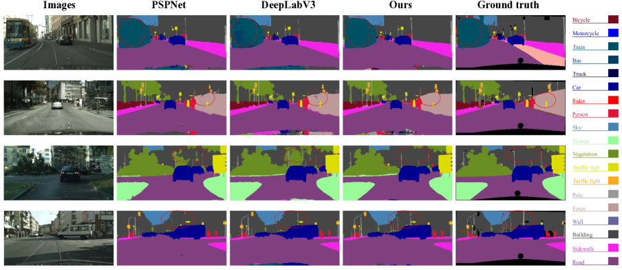
Figure 5: Qualitative comparisons with DeepLab-V3 [7] and PSPNet [47]. The red circles mark where our model is particularly superior to other methods.

Method	mIoU (%)
Baseline	75.8
+ NB	78.4
+ APNB	78.6
+ Common fusion	76.5
+ FNB	77.3
+ AFNB	77.1
+ Common fusion + NB	79.0
+ FNB + NB	79.7
+ AFNB + APNB (Full)	79.9

Table 6: Ablation study on the validation set of Cityscapes about APNB and AFNB. “+ $Module$” means add “$Module$” to the Baseline model.

In this section, we give extensive experiments to verify the efficacy of our main method. We also give several design choices and show their influences on the results. All the following experiments adopt ResNet-101 as the backbone, trained on the fine-annotated training set of Cityscapes for 60K iterations.

Efficacy of the APNB and AFNB. Our network has two prominent components: APNB and AFNB. The following will evaluate the efficacy of each and the integration of both. The Baseline network is basically a FCN-like ResNet-101 network with a deep supervision branch. By adding a non-local block (+ NB) before the classifier to the Baseline model, the performance is improved by 2.6% (75.8% $\rightarrow$ 78.4%), as shown in Tab. 6. By replacing the normal non-local block with our APNB (+ APNB), the performance is slightly better (78.4% $\rightarrow$ 78.6%).

When adding a common fusion module (+ Common Fusion) from $\mathrm{Stage4}$ to $\mathrm{Stage5}$: $\mathrm{Stage5}+\mathrm{ReLU(BatchNorm(Conv(Stage4)))}$ to Baseline model, we also achieve a good improvement compared to the Baseline (75.8% $\rightarrow$ 76.5%). This phenomenon verifies the usefulness of the strategy that fuses the features from the last two stages. Replacing the common fusion module with our proposed Fusion Non-local Block (+ FNB), the performance is further boosted at 0.8% (76.5% $\rightarrow$ 77.3%). Likewise, changing FNB to AFNB (+ AFNB) reduces the computation considerably at the cost of a minor performance decrease (77.3% $\rightarrow$ 77.1%).

To study whether the fusion strategy could further boost the highly competitive + NB model, we add Common fusion to + NB model (+ Common fusion + NB) and achieve 0.6% performance improvement (78.4% $\rightarrow$ 79.0%). Using both the fusion non-local block and typical non-local block (+ FNB + NB) can improve the performance of 79.7%. Using the combination of APNB and AFNB, namely our asymmetric non-local neural network (+ AFNB + APNB (Full) in Fig. 3), achieves the best performance of 79.9%, demonstrating the efficacy of APNB and AFNB.

Selection of Sampling Methods. As discussed in Sec. 3.2, the selection of the sampling module has a great impact on the performance of APNB. Normal sampling strategies include: max, average and random. When integrated into spatial pyramid pooling, there goes another three strategies: pyramid max, pyramid average and pyramid random. We thereupon conduct several experiments to study their effects by combining them with APNB. As shown in Tab. 7, average sampling performs better than max and random sampling, which conforms to the conclusion drawn in [47]. We reckon it is because the resulted sampling points are more informative by receiving the provided information of all the input locations inside the average sampling kernel, when compared to the other two. This explanation could also be transferred to pyramid settings. Comparing average sampling and pyramid sampling under the same number of anchor points (third row vs. the last row), we can surely find pyramid pooling is a very key factor that contributes to the significant performance boost.

Influence of the Anchor Points Numbers. In our case, the output sizes of the pyramid pooling layers determine the total number of anchor points, which influence the efficacy of APNB. To investigate the influence, we perform the following experiments by altering the pyramid average pooling output sizes: $(1,2,3,6)$, $(1,3,6,8)$ and $(1,4,8,12)$. As shown in Tab. 7, it is clear that more anchor points improve the performance with the cost of increasing computation. Considering this trade-off between efficacy and efficiency, we opt to choose $(1,3,6,8)$ as our default setting.

Sampling method	$n$	${\color[rgb]{0,0,1}S}$	mIoU (%)
random	15	225	78.2
max	15	225	78.1
average	15	225	78.4
pyramid random	1,2,3,6	50	78.8
pyramid max	1,2,3,6	50	79.1
pyramid average	1,2,3,6	50	79.3
pyramid average	1,3,6,8	110	79.9
pyramid average	1,4,8,12	225	80.1

Table 7: Ablation study on the validation set of Cityscapes in terms of sampling methods and anchor point number. “$n$” column represents the output width/height of a pooling layer. Note when implementing random and pyramid random, we use the $\mathrm{numpy.random.choice}$ function to randomly sample $n^{2}$ anchor points from all possible locations. “$S$” column means the total number of the anchor points.

5 Conclusion

In this paper, we propose an asymmetric non-local neural network for semantic segmentation. The core contribution of asymmetric non-local neural network is the asymmetric pyramid non-local block, which can dramatically improve the efficiency and decrease the memory consumption of non-local neural blocks without sacrificing the performance. Besides, we also propose asymmetric fusion non-local block to fuse features of different levels. The asymmetric fusion non-local block can explore the long range spatial relevance among features of different levels, which demonstrates a considerable performance improvement over a strong baseline. Comprehensive experimental results on the Cityscapes, ADE20K and PASCAL Context datasets show that our work achieves the new state-of-the-art performance. In the future, we will apply asymmetric non-local neural networks to other vision tasks.

Appendix A Quantitative comparisons on COCO-Stuff-10K and NYUD-V2

Following the training and evaluation protocols of DeepLab-V2 [6] and RefineNet [18], our method achieves competitive results on the two datasets using single scale whole image testing, as shown in Tab. 8. As NYUD-V2 [29] is a small benchmark and COCO-Stuff-10K is quite challenging and large, these results further verify the effectiveness of our method on both small and large benchmarks.

Method	Backbone	mIoU (%)	Method	Backbone	mIoU (%)
RefineNet [18]	ResNet-101	33.6	Piecewise [19]	VGG16	40.6
CCL [11]	ResNet-101	35.7	RefineNet [18]	ResNet-101	43.6
Ours	ResNet-101	37.2	Ours	ResNet-101	44.4

Table 8: Comparisons on COCO-Stuff-10K (Left) and NYUD-V2 (Right) datasets. Results of the competing methods are taken from their papers.

Appendix B More ablation results

Qualitative comparisons. We also give the qualitative comparisons of our Full (+ AFNB + APNB) method with other variants of our model in Fig. 6. In summary, our Full method shows the best semantic consistency and the least inconsistency artifacts while +AFNB and +APNB fail in some cases. The results also indicate AFNB and APNB is complementary to each other and the combination of them is beneficial to improve the performance.

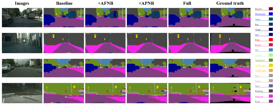
Figure 6: Qualitative comparisons among Full model and other variants of our model. The red circles indicate where Full model is superior to other model variants.

Selection of the fusing layers. Fusing features from multi-levels is effective in many computer vision tasks. However, it still requires a lot of trials to find a good combination of the fusing layers. For semantic segmentation, the last several layers of the network contain plenty of features with semantic information, which is critical for better performance. Hence, we only combine the features from the shallow layers to the deep layers in a top-down manner. The responses are summed up if a certain layer receives more than two fusion invitations. The results are listed in Tab. 9. An obvious conclusion is that fusing only the features of $\mathrm{Stage4}$ and $\mathrm{Stage5}$ brings a considerable improvement while keep fusing more layers will only hurt the performance.

We conclude a possible intuitive reason: features from the early stages are generic to most tasks, while the last two are task-specific. Therefore, merging the features of the last several stages is more effective for a specific task. In the supplementary materials, we compare the feature visualizations of the outputs of all 5 stages of network trained on segmentation benchmark Cityscapes [9] and of that trained on classification benchmark ImageNet [10], using the same backbone network ResNet-101 to demonstrate our guess.

As can be seen in Fig. 7, we compare the feature visualizations of the outputs of all 5 stages of network trained on segmentation benchmark Cityscapes [9] (Lower) and of that trained on classification benchmark ImageNet [10] (Upper), using the same backbone network ResNet-101. Comparing the two networks’ feature visualizations of the same stage, the features are quite similar in the first three stages while differs hugely in the last two. This observation accord with our guess. Note our experiment results partially conforms to the conclusions in ExFuse [46], further validating the effectiveness of fusing only the last two stages.

Method	Fusing layers	mIoU (%)
Baseline	–	75.8
AFNB	4 & 5	77.1
AFNB	3 & 5, 4 & 5	76.7
AFNB	2 & 5, 3 & 5, 4 & 5	76.2

Table 9: Ablation study on the validation set of Cityscapes in terms of the selection of layers to be fused. “4 & 5” means fusing the features of $\mathrm{Stage4}$ and $\mathrm{Stage5}$. Others likewise.

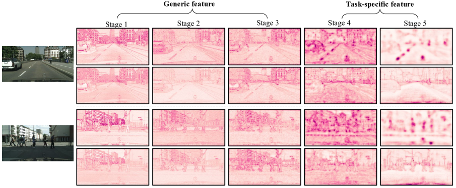
Figure 7: Feature visualization of different stages on ResNet-101. The Upper row represents visualizations from network trained on classification dataset ImageNet [10]. The Lower row represents visualizations from network trained on scene segmentation dataset Cityscapes [9].

Appendix C Discussions

We’ve conducted extensive experiments to summarize some experiences about semantic segmentation. As known, deep networks are fantastic tools but also need very careful tuning. The tuning process is extremely painful when it comes to semantic segmentation as there are many factors and the training process is very time and resources consuming. So we plan to share some experiences to the interested readers as references. But please do note these experiences are not as thorough as those in the main draft and it’s very possible that some may not suit your cases.

• We found the types of graphic cards, pytorch versions, CUDA versions and NVIDIA driver versions may influence the performances. In our case, we found the same model trained on a workstation with 8 $\times$ Titan V is around 0.5 mIoU better than it trained on another machine with 8 $\times$ Titan Xp.

• The architecture of AFNB needs careful modifications to make AFNB work better. For example, we found adding a batch normalization layer after $W_{o}$ helps a lot when using AFNB alone while may not help on the Full model. We suspect there is a theoretical reason here and we’re working to solve this issue. However, we found APNB is quite stable across a variaty of architectures.

• It seems that learning rate is important for segmentation models because we observe that the performance is boosted tremendously in the last 1/4 of training iterations. We also found that changing the initial learning rate has a great impact on the performance. We strongly suggest those, who are new to this task, refer to the learning rate configurations of the published methods that are mostly similar to your own method in architecture.

• Using larger training iterations while keeping other configurations identical doesn’t always improve the performance. In fact, changing training iterations is related to change the learning rate during training as we mainly adopt poly learning decay method in semantic segmentation.

References

- [1] Vijay Badrinarayanan, Alex Kendall, and Roberto Cipolla. Segnet: A deep convolutional encoder-decoder architecture for image segmentation. IEEE Trans. Pattern Anal. Mach. Intell., 39(12):2481–2495, 2017.
- [2] Antoni Buades, Bartomeu Coll, and Jean-Michel Morel. A non-local algorithm for image denoising. In Proc. CVPR, pages 60–65, 2005.
- [3] Holger Caesar, Jasper R. R. Uijlings, and Vittorio Ferrari. Coco-stuff: Thing and stuff classes in context. In Proc. CVPR, pages 1209–1218, 2018.
- [4] Siddhartha Chandra and Iasonas Kokkinos. Fast, exact and multi-scale inference for semantic image segmentation with deep gaussian crfs. In Proc. ECCV, pages 402–418, 2016.
- [5] Liang-Chieh Chen, George Papandreou, Iasonas Kokkinos, Kevin Murphy, and Alan L. Yuille. Semantic image segmentation with deep convolutional nets and fully connected crfs. In Proc. ICLR, 2015.
- [6] Liang-Chieh Chen, George Papandreou, Iasonas Kokkinos, Kevin Murphy, and Alan L. Yuille. Deeplab: Semantic image segmentation with deep convolutional nets, atrous convolution, and fully connected crfs. IEEE Trans. Pattern Anal. Mach. Intell., 40(4):834–848, 2018.
- [7] Liang-Chieh Chen, George Papandreou, Florian Schroff, and Hartwig Adam. Rethinking atrous convolution for semantic image segmentation. CoRR, abs/1706.05587, 2017.
- [8] Liang-Chieh Chen, Yukun Zhu, George Papandreou, Florian Schroff, and Hartwig Adam. Encoder-decoder with atrous separable convolution for semantic image segmentation. In Proc. ECCV, pages 833–851, 2018.
- [9] Marius Cordts, Mohamed Omran, Sebastian Ramos, Timo Rehfeld, Markus Enzweiler, Rodrigo Benenson, Uwe Franke, Stefan Roth, and Bernt Schiele. The cityscapes dataset for semantic urban scene understanding. In Proc. CVPR, pages 3213–3223, 2016.
- [10] Jia Deng, Wei Dong, Richard Socher, Li-Jia Li, Kai Li, and Fei-Fei Li. Imagenet: A large-scale hierarchical image database. In Proc. CVPR, pages 248–255, 2009.
- [11] Henghui Ding, Xudong Jiang, Bing Shuai, Ai Qun Liu, and Gang Wang. Context contrasted feature and gated multi-scale aggregation for scene segmentation. In Proc. CVPR, pages 2393–2402, 2018.
- [12] Kaiming He, Xiangyu Zhang, Shaoqing Ren, and Jian Sun. Spatial pyramid pooling in deep convolutional networks for visual recognition. IEEE Trans. Pattern Anal. Mach. Intell., 37(9):1904–1916, 2015.
- [13] Kaiming He, Xiangyu Zhang, Shaoqing Ren, and Jian Sun. Deep residual learning for image recognition. In Proc. CVPR, pages 770–778, 2016.
- [14] Tsung-Wei Ke, Jyh-Jing Hwang, Ziwei Liu, and Stella X. Yu. Adaptive affinity fields for semantic segmentation. In Proc. ECCV, pages 605–621, 2018.
- [15] John D. Lafferty, Andrew McCallum, and Fernando C. N. Pereira. Conditional random fields: Probabilistic models for segmenting and labeling sequence data. In Proc. ICML, pages 282–289, 2001.
- [16] Svetlana Lazebnik, Cordelia Schmid, and Jean Ponce. Beyond bags of features: Spatial pyramid matching for recognizing natural scene categories. In Proc. CVPR, pages 2169–2178, 2006.
- [17] Xiaodan Liang, Hongfei Zhou, and Eric Xing. Dynamic-structured semantic propagation network. In Proc. CVPR, pages 752–761, 2018.
- [18] Guosheng Lin, Anton Milan, Chunhua Shen, and Ian D. Reid. Refinenet: Multi-path refinement networks for high-resolution semantic segmentation. In Proc. CVPR, pages 5168–5177, 2017.
- [19] Guosheng Lin, Chunhua Shen, Anton van den Hengel, and Ian D. Reid. Efficient piecewise training of deep structured models for semantic segmentation. In Proc. CVPR, pages 3194–3203, 2016.
- [20] Wei Liu, Andrew Rabinovich, and Alexander C. Berg. Parsenet: Looking wider to see better. CoRR, abs/1506.04579, 2015.
- [21] Roozbeh Mottaghi, Xianjie Chen, Xiaobai Liu, Nam-Gyu Cho, Seong-Whan Lee, Sanja Fidler, Raquel Urtasun, and Alan Yuille. The role of context for object detection and semantic segmentation in the wild. In Proc. CVPR, 2014.
- [22] Hyeonwoo Noh, Seunghoon Hong, and Bohyung Han. Learning deconvolution network for semantic segmentation. In Proc. ICCV, pages 1520–1528, 2015.
- [23] Adam Paszke, Sam Gross, Soumith Chintala, Gregory Chanan, Edward Yang, Zachary DeVito, Zeming Lin, Alban Desmaison, Luca Antiga, and Adam Lerer. Automatic differentiation in pytorch. 2017.
- [24] Chao Peng, Xiangyu Zhang, Gang Yu, Guiming Luo, and Jian Sun. Large kernel matters - improve semantic segmentation by global convolutional network. In Proc. CVPR, pages 1743–1751, 2017.
- [25] Olaf Ronneberger, Philipp Fischer, and Thomas Brox. U-net: Convolutional networks for biomedical image segmentation. In Proc. MICCAI, pages 234–241, 2015.
- [26] Evan Shelhamer, Jonathan Long, and Trevor Darrell. Fully convolutional networks for semantic segmentation. IEEE Trans. Pattern Anal. Mach. Intell., 39(4):640–651, 2017.
- [27] Mennatullah Siam, Sara Elkerdawy, Martin Jägersand, and Senthil Yogamani. Deep semantic segmentation for automated driving: Taxonomy, roadmap and challenges. In Proc. ITSC, pages 1–8, 2017.
- [28] Mennatullah Siam, Mostafa Gamal, Moemen Abdel-Razek, Senthil Yogamani, Martin Jägersand, and Hong Zhang. A comparative study of real-time semantic segmentation for autonomous driving. In CVPR workshop, pages 587–597, 2018.
- [29] Nathan Silberman, Derek Hoiem, Pushmeet Kohli, and Rob Fergus. Indoor segmentation and support inference from RGBD images. In Proc. ECCV, pages 746–760, 2012.
- [30] Ashish Vaswani, Noam Shazeer, Niki Parmar, Jakob Uszkoreit, Llion Jones, Aidan N. Gomez, Lukasz Kaiser, and Illia Polosukhin. Attention is all you need. In Proc. NeurIPS, pages 6000–6010, 2017.
- [31] Raviteja Vemulapalli, Oncel Tuzel, Ming-Yu Liu, and Rama Chellappa. Gaussian conditional random field network for semantic segmentation. In Proc. CVPR, pages 3224–3233, 2016.
- [32] Panqu Wang, Pengfei Chen, Ye Yuan, Ding Liu, Zehua Huang, Xiaodi Hou, and Garrison W. Cottrell. Understanding convolution for semantic segmentation. In Proc. WACV, pages 1451–1460, 2018.
- [33] Xiaolong Wang, Ross B. Girshick, Abhinav Gupta, and Kaiming He. Non-local neural networks. In Proc. CVPR, pages 7794–7803, 2018.
- [34] Zifeng Wu, Chunhua Shen, and Anton van den Hengel. Wider or deeper: Revisiting the resnet model for visual recognition. CoRR, abs/1611.10080, 2016.
- [35] Tete Xiao, Yingcheng Liu, Bolei Zhou, Yuning Jiang, and Jian Sun. Unified perceptual parsing for scene understanding. In Proc. ECCV, pages 432–448, 2018.
- [36] Maoke Yang, Kun Yu, Chi Zhang, Zhiwei Li, and Kuiyuan Yang. Denseaspp for semantic segmentation in street scenes. In Proc. CVPR, pages 3684–3692, 2018.
- [37] Ansheng You, Xiangtai Li, Zhen Zhu, and Yunhai Tong. Torchcv: A pytorch-based framework for deep learning in computer vision. https://github.com/donnyyou/torchcv, 2019.
- [38] Changqian Yu, Jingbo Wang, Chao Peng, Changxin Gao, Gang Yu, and Nong Sang. Bisenet: Bilateral segmentation network for real-time semantic segmentation. In Proc. ECCV, pages 334–349, 2018.
- [39] Changqian Yu, Jingbo Wang, Chao Peng, Changxin Gao, Gang Yu, and Nong Sang. Learning a discriminative feature network for semantic segmentation. In Proc. CVPR, pages 1857–1866, 2018.
- [40] Fisher Yu and Vladlen Koltun. Multi-scale context aggregation by dilated convolutions. CoRR, abs/1511.07122, 2015.
- [41] Fisher Yu, Dequan Wang, Evan Shelhamer, and Trevor Darrell. Deep layer aggregation. In Proc. CVPR, pages 2403–2412, 2018.
- [42] Yuhui Yuan and Jingdong Wang. Ocnet: Object context network for scene parsing. CoRR, abs/1809.00916, 2018.
- [43] Hang Zhang, Kristin J. Dana, Jianping Shi, Zhongyue Zhang, Xiaogang Wang, Ambrish Tyagi, and Amit Agrawal. Context encoding for semantic segmentation. In Proc. CVPR, pages 7151–7160, 2018.
- [44] Han Zhang, Ian J. Goodfellow, Dimitris N. Metaxas, and Augustus Odena. Self-attention generative adversarial networks. In Proc. ICML, pages 7354–7363, 2019.
- [45] Rui Zhang, Sheng Tang, Yongdong Zhang, Jintao Li, and Shuicheng Yan. Scale-adaptive convolutions for scene parsing. In Proc. ICCV, pages 2050–2058, 2017.
- [46] Zhenli Zhang, Xiangyu Zhang, Chao Peng, Xiangyang Xue, and Jian Sun. Exfuse: Enhancing feature fusion for semantic segmentation. In Proc. CVPR, pages 273–288, 2018.
- [47] Hengshuang Zhao, Jianping Shi, Xiaojuan Qi, Xiaogang Wang, and Jiaya Jia. Pyramid scene parsing network. In Proc. CVPR, pages 6230–6239, 2017.
- [48] Hengshuang Zhao, Yi Zhang, Shu Liu, Jianping Shi, Chen Change Loy, Dahua Lin, and Jiaya Jia. Psanet: Point-wise spatial attention network for scene parsing. In Proc. ECCV, pages 270–286, 2018.
- [49] Shuai Zheng, Sadeep Jayasumana, Bernardino Romera-Paredes, Vibhav Vineet, Zhizhong Su, Dalong Du, Chang Huang, and Philip H. S. Torr. Conditional random fields as recurrent neural networks. In Proc. ICCV, pages 1529–1537, 2015.
- [50] Bolei Zhou, Hang Zhao, Xavier Puig, Sanja Fidler, Adela Barriuso, and Antonio Torralba. Scene parsing through ADE20K dataset. In Proc. CVPR, pages 5122–5130, 2017.
- [51] Yu Zhou, Xiang Bai, Wenyu Liu, and Longin Jan Latecki. Similarity fusion for visual tracking. International Journal of Computer Vision, 118(3):337–363, 2016.
- [52] Yuyin Zhou, Zhe Li, Song Bai, Chong Wang, Xinlei Chen, Mei Han, Elliot Fishman, and Alan Yuille. Prior-aware neural network for partially-supervised multi-organ segmentation. In Proc. ICCV, 2019.
- [53] Yuyin Zhou, Yan Wang, Peng Tang, Song Bai, Wei Shen, Elliot Fishman, and Alan Yuille. Semi-supervised 3d abdominal multi-organ segmentation via deep multi-planar co-training. In Proc. WACV, pages 121–140, 2019.