On the effects of an impurity in an Ising-$XXZ$ diamond chain on the thermal entanglement, on the quantum coherence and on the quantum teleportation

Abstract

The effects of an impurity plaquette on the thermal quantum correlations measurement by the concurrence, on the quantum coherence quantified by the recently proposed $l_{1}$-norm of coherence and on the quantum teleportation in a Ising-$XXZ$ diamond chain are discussed. Such an impurity is formed by the $XXZ$ interaction between the interstitial Heisenberg dimers and the nearest-neighbor Ising coupling between the nodal and interstitial spins. All the interaction parameters are different from those of the rest of the chain. By tailoring them, the quantum entanglement and quantum coherence can be controlled and tuned. Therefore, the quantum resources -thermal entanglement and quantum coherence- of the model exhibit a clear performance improvement in comparison to the original model without impurities. We also demonstrate that the quantum teleportation can be tuned by its inclusion. The thermal teleportation is modified in significant way as well, and a strong increase in average fidelity is observed. We furnish the exact solution by the use of the transfer-matrix method.

I Introduction

The quantum resource theories st ; st-1 play a central role in the quantum information processing. In particular, quantum coherence and entanglement are resources for quantum technological applications i.e., quantum communication and quantum computation bra ; Bene ; amico . Recently, the role of the quantum coherence on Heisenberg spin models has been considered rada ; fan ; wei . Furthermore, recent research reveals that these resources have a close connection with each otheradesso . On the other hand, quantum entanglement is one of the most fascinating features of the quantum theory, and it has been regarded as an essential physical resource for quantum computation and quantum information. The Heisenberg chain is one of the simplest quantum system which exhibits entanglement. For this reason, the Heisenberg spin models have been extensively studied in condensed matter systemskam . Also, many schemes of teleportation via thermal entanglement states have been reportedyeo . In the context of the spin-1/2 Heisenberg model with a diamond chain structure, a novel class of the simplified versions of the so-called Ising-Heisenberg diamond chain was introduced in Ref. strec . The various thermodynamic properties of it have been extensively investigatedrojas . Recently, the thermal quantum entanglement in some exactly solvable Ising-Heisenberg diamond chains have been extensively analyzed and discussed moi ; cheng ; rojas-1 ; rojas-2 . More recently, Rojas $et\,al$ moi-1 discussed the entangled state teleportation through a couple of quantum channels composed of $XXZ$ dimers in an Ising-$XXZ$ diamond chain.

Impurities play an important role in solid state physics falk . Even a small defect may changes the physical properties of the quantum system. In recent years, the study of the spin chains with impurities has attracted much attention fuku ; xuchu , including the various kinds of the spin chains with a magnetic impurityfu . In Ref. rojas-3 , the tuning of the thermal entanglement in a Ising-$XXZ$ diamond chain with two impurities was addressed.

Motivated by these mentioned developments, the present work is addressed to a detailed investigation on the influence of an impurity plaquette inserted in an Ising-$XXZ$ diamond chain. Such an impurity spin is defined by a local change in the nearest-neighbor couplings. We will focus on the analysis of the thermal entanglement and on the quantum coherence in this impurity embedded environment. It is shown that the impurities parameters can generate a significant enhancement on the entanglement and on the quantum coherence. Besides, we study the teleportation of an unknown state using a couple of impure Heisenberg dimers embedded in an Ising-$XXZ$ diamond chain in thermal equilibrium as a quantum channel. The effects due to it as well as those due to the parameters of a Heisenberg interaction, an Ising interaction and magnetic fields in the fidelity and average fidelity are obtained analytically.

The organization of this article is as follows. In Sec. II we introduce the Ising-XXZ model with an impurity. In Sec.III, we obtain the exact solution of the model via the transfer-matrix approach and its dimer (two-qubit) reduced density operator. In Sec.IV, we discuss the thermal entanglement and quantum coherence of the impurity Heisenberg reduced density operator of the model. In Sec.V, we study the effects of the impurity parameters on teleportation scheme. We evaluate the fidelity and average fidelity. Finally, the concluding remarks are given in Sec. VI.

II The Model

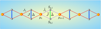
Figure 1: (Color online) A schematic representation of an Ising-$XXZ$ diamond chain with one impurity inserted in the $i$-th block of the primitive unit cell.

In this section, we introduce the hamiltonian of the spin-1/2 Ising-$XXZ$ model on a diamond chain with one plaquette impurity under an external magnetic field, $h$. The model consists on the interstitial Heisenberg spins $(S_{a,i},\>S_{b,i})$ and Ising spins $(\sigma_{i},\>\sigma_{i+1})$ located in the nodal site, as shown in Fig. 1. The total hamiltonian of the model may be written as

$$\mathcal{H}=\sum_{i=1}^{N}\mathcal{H}_{i},$$

where $\mathcal{H}_{i}=\mathcal{H}_{i}^{host}+\mathcal{H}_{i}^{imp},$ and the host hamiltonian $\mathcal{H}_{i}^{host}$ can be expressed as

$$\begin{array}[]{cl}\mathcal{H}_{i}^{host}=&J\left(\mathbf{S}_{a,i},\mathbf{S}_{b,i}\right)_{\Delta}+J_{1}\left(S_{a,i}^{z}+S_{b,i}^{z}\right)\left(\mu_{i}+\mu_{i+1}\right)\\ &-h\left(S_{a,i}^{z}+S_{b,i}^{z}\right)-\frac{h}{2}\left(\mu_{i}+\mu_{i+1}\right).\\ &\mathrm{for}\>i=1,2,\ldots,r-1,r+1,\ldots,N\end{array}$$

On the other hand, the impurity induced hamiltonian $\mathcal{H}_{i}^{imp}$, is defined by

$$\begin{array}[]{cl}\mathcal{H}_{i}^{imp}=&\widetilde{J}\left(\mathbf{S}_{a,i},\mathbf{S}_{b,i}\right)_{\widetilde{\Delta}}+\widetilde{J}_{1}\left(S_{a,i}^{z}+S_{b,i}^{z}\right)\left(\mu_{i}+\mu_{i+1}\right)\\ &-h\left(S_{a,i}^{z}+S_{b,i}^{z}\right)-\frac{h}{2}\left(\mu_{i}+\mu_{i+1}\right),\\ &\mathrm{for}\>i=r\;,\end{array}$$

where the parameters $J$ and $\Delta$ denote the $XXZ$ interaction within the Heisenberg dimer, the nodal-interstitial spins interaction are represented by the Ising-type exchanges $J_{1}$, $h$ denotes the longitudinal magnetic field in the $z$ direction and the impurity parameters are given by $\widetilde{J}=J\left(1+\alpha\right)$, $\widetilde{\Delta}=\Delta\left(1+\gamma\right)$ and $\widetilde{J}_{1}=J_{1}\left(1+\eta\right)$.

After straightforward calculations, the eigenvalues for the $XXZ$ dimer of the above host hamiltonian $\mathcal{H}_{i}^{host}$ can be obtained as

$$\mathcal{E}_{i1,i4}= \frac{J\Delta}{4}\pm\left(J_{1}\mp\frac{h}{2}\right)(\mu_{i}+\mu_{i+1})\mp h,$$

$$\mathcal{E}_{i2,i3}= -\frac{J\Delta}{4}\pm\frac{J_{1}}{2}-\frac{h}{2}(\sigma_{i}+\sigma_{i+1}),$$

where their corresponding eigenstates in terms of the standard basis $\{|00\rangle,|01\rangle,|10\rangle,|11\rangle\}$ are given, respectively, by

$$|\varphi_{i1}\rangle= |00\rangle_{i},$$ (1)

$$|\varphi_{i2}\rangle= \frac{1}{\sqrt{2}}\left(|01\rangle_{i}+|10\rangle_{i}\right),$$ (2)

$$|\varphi_{i3}\rangle= \frac{1}{\sqrt{2}}\left(|01\rangle_{i}-|10\rangle_{i}\right),$$ (3)

$$|\varphi_{i4}\rangle= |11\rangle_{i}\;.$$ (4)

Analogously to the impurity dimer, the eigenvalues of the $\mathcal{H}_{i}^{imp}$ are

$$\mathcal{\widetilde{E}}_{i1,i4}= \frac{\widetilde{J}\widetilde{\Delta}}{4}\pm\left(\widetilde{J}_{1}\mp\frac{h}{2}\right)(\mu_{i}+\mu_{i+1})\mp h,$$

$$\mathcal{\widetilde{E}}_{i2,i3}= -\frac{\widetilde{J}\widetilde{\Delta}}{4}\pm\frac{\widetilde{J}_{1}}{2}-\frac{h}{2}(\sigma_{i}+\sigma_{i+1}),$$

and the corresponding eigenstates are

$$|\widetilde{\varphi}_{i1}\rangle= |00\rangle_{i},$$ (5)

$$|\widetilde{\varphi}_{i2}\rangle= \frac{1}{\sqrt{2}}\left(|01\rangle_{i}+|10\rangle_{i}\right),$$ (6)

$$|\widetilde{\varphi}_{i3}\rangle= \frac{1}{\sqrt{2}}\left(|01\rangle_{i}-|10\rangle_{i}\right),$$ (7)

$$|\widetilde{\varphi}_{i4}\rangle= |11\rangle_{i}.$$ (8)

Here, $r=i$.

III The partition function and the density operator

In order to study the thermal entanglement, the quantum coherence and the quantum teleportation, we first must obtain a partition function for a diamond chain. This model can be solved exactly through the transfer-matrix approach baxter . In order to summarize this approach we will define the following operator, as a function of Ising spin particles $\mu_{i}$ and $\mu_{i+1}$,

$$\varrho(\mu_{i},\mu_{i+1})=\sum_{i=1}^{4}\mathrm{e}^{-\beta\mathcal{E}_{ij}(\mu_{i},\mu_{i+1})}|\varphi_{ij}\rangle\langle\varphi_{ij}|\;,$$ (9)

where $\beta=1/k_{B}T$, $k_{B}$ is the Boltzmann’s constant and $T$ is the absolute temperature.

Straightforwardly, we can obtain the Boltzmann factor by tracing out over the two-qubit operator,

$$w(\mu_{i},\mu_{i+1})=\mathrm{tr}_{ab}\left(\widetilde{\varrho}(\mu_{i},\mu_{i+1})\right)=\sum_{j=1}^{4}\mathrm{e}^{-\beta\mathcal{E}_{ij}(\mu_{i},\mu_{i+1})}\;.$$ (10)

The Boltzmann factor for an impurity is given by

$$\widetilde{w}(\mu_{i},\mu_{i+1})=\sum_{j=1}^{4}\mathrm{e}^{-\beta\mathcal{\widetilde{E}}_{ij}(\mu_{i},\mu_{i+1})}\;,$$

where $i=r$. The Ising-XXZ diamond chain partition function can be written in terms of the Boltzmann factors,

$$Z_{N}= \sum_{\{\mu\}}w(\mu_{1},\mu_{2})\ldots w(\mu_{r-1},\mu_{r})\widetilde{w}(\mu_{r},\mu_{r+1})\times$$

$$w(\mu_{r+1},\mu_{r+2})\ldots w(\mu_{N},\mu_{1})\;.$$ (11)

Using the transfer-matrix notation, we can write the partition function of the diamond chain straightforwardly by $Z_{N}=\mathrm{tr}\left(\widetilde{W}W^{N-1}\right),$ where the transfer-matrix is expressed as

$$W=\left[\begin{array}[]{cc}w(\frac{1}{2},\frac{1}{2})&w(\frac{1}{2},-\frac{1}{2})\\ w(-\frac{1}{2},\frac{1}{2})&w(-\frac{1}{2},-\frac{1}{2})\end{array}\right]\;.$$ (12)

A similar formula can also be derived for the transfer-matrix $\widetilde{W}$ for the impurity case, namely

$$\widetilde{W}=\left[\begin{array}[]{cc}\widetilde{w}(\frac{1}{2},\frac{1}{2})&\widetilde{w}(\frac{1}{2},-\frac{1}{2})\\ \widetilde{w}(-\frac{1}{2},\frac{1}{2})&\widetilde{w}(-\frac{1}{2},-\frac{1}{2})\end{array}\right]\;.$$

In it, the transfer matrix elements are denoted by $w_{++}\equiv w(\frac{1}{2},\frac{1}{2})$, $w_{+-}\equiv w(\frac{1}{2},-\frac{1}{2})$ and $w_{--}\equiv w(-\frac{1}{2},-\frac{1}{2})$. After performing the diagonalization of the transfer matrix (12), the eigenvalues are found, that is,

$$\Lambda_{\pm}=\frac{w_{++}+w_{--}\pm Q}{2}\;.$$ (13)

It was assumed that $Q=\sqrt{\left(w_{++}-w_{--}\right)^{2}+4w_{+-}^{2}}$. Therefore, the partition function for finite chain under periodic boundary conditions is given by

$$Z_{N}=a\Lambda_{+}^{N-1}+d\Lambda_{-}^{N-1}\;,$$ (14)

where

$$\begin{array}[]{cc}a=&\frac{4w_{+-}\widetilde{w}_{+-}+\left(w_{++}-w_{--}\right)\left(\widetilde{w}_{++}-\widetilde{w}_{--}\right)+Q\left(\widetilde{w}_{++}+\widetilde{w}_{--}\right)}{2Q},\\ d=&\frac{-4w_{+-}\widetilde{w}_{+-}-\left(w_{++}-w_{--}\right)\left(\widetilde{w}_{++}-\widetilde{w}_{--}\right)+Q\left(\widetilde{w}_{++}+\widetilde{w}_{--}\right)}{2Q}\;.\end{array}$$

In the thermodynamic limit, the partition function will be simplified. Thus we obtain $Z_{N}=a\Lambda_{+}^{N-1}$. Now, we are interested in the thermal quantum correlations and in the quantum teleportation. To reach out our goal it is essential to obtain the reduced density operators $\widetilde{\rho}$ of the dimer Heisenberg impurity.

III.1 Two-qubit operator

In order to calculate the thermal average of the two-qubit operator corresponding to an impurity, also called reduced two-qubit density operator, we will use the approach recently studied in Ref. rojas-3 . This way, we will define the operator $\widetilde{\varrho}$ for an impurity as a function of the Ising particles $\mu_{r}$ and $\mu_{r+1}$, that is,

$$\widetilde{\varrho}(\mu_{r},\mu_{r+1})=\left[\begin{array}[]{cccc}\widetilde{\varrho}_{1,1}&0&0&0\\ 0&\widetilde{\varrho}_{2,2}&\widetilde{\varrho}_{2,3}&0\\ 0&\widetilde{\varrho}_{2,3}&\widetilde{\varrho}_{2,2}&0\\ 0&0&0&\widetilde{\varrho}_{4,4}\end{array}\right]\;,$$ (15)

where the elements of the two-qubit operator are given by

$$\widetilde{\varrho}_{1,1}(\mu_{r},\mu_{r+1})= \mathrm{e}^{-\beta\mathcal{\widetilde{E}}_{r1}(\mu_{r},\mu_{r+1})},$$

$$\widetilde{\varrho}_{2,2}(\mu_{r},\mu_{r+1})= \frac{1}{2}\left(\mathrm{e}^{-\beta\mathcal{\widetilde{E}}_{r2}(\mu_{r},\mu_{r+1})}+\mathrm{e}^{-\beta\mathcal{\widetilde{E}}_{r3}(\mu_{r},\mu_{r+1})}\right),$$

$$\widetilde{\varrho}_{2,3}(\mu_{r},\mu_{r+1})= \frac{1}{2}\left(\mathrm{e}^{-\beta\mathcal{\widetilde{E}}_{r2}(\mu_{r},\mu_{r+1})}-\mathrm{e}^{-\beta\mathcal{\widetilde{E}}_{r3}(\mu_{r},\mu_{r+1})}\right),$$

$$\widetilde{\varrho}_{4,4}(\mu_{r},\mu_{r+1})= \mathrm{e}^{-\beta\mathcal{\widetilde{E}}_{r4}(\mu_{r},\mu_{r+1})}\;.$$

The thermal average for each two-qubit Heisenberg operator will be used to construct the reduced density operator.

III.2 The reduced density operator for the impurity

The elements of the reduced density operator, $\widetilde{\rho}_{k,l}$, for an impurity localized in the $r$th block (unit cell), can be defined by

$$\widetilde{\rho}_{k,l}= \frac{1}{Z_{N}}\sum_{\{\mu\}}w(\mu_{1},\mu_{2})\ldots w(\mu_{r-1},\mu_{r})\widetilde{\varrho}_{k,l}(\mu_{r},\mu_{r+1})\times$$

$$w(\mu_{r+1},\mu_{r+2})\ldots w(\mu_{N},\mu_{1})\;.$$ (16)

Using the transfer-matrix approach, $\widetilde{\rho}_{k,l}$ can be alternatively rewritten as

$$\tilde{\rho}_{k,l}=\frac{1}{Z_{N}}\mathrm{tr}\left(W^{r-1}\widetilde{P}_{k,l}W^{N-r}\right)=\frac{1}{Z_{N}}\mathrm{tr}\left(\widetilde{P}_{k,l}W^{N-1}\right)\;,$$ (17)

where

$$\widetilde{P}_{k,l}=\left[\begin{array}[]{cc}\widetilde{\varrho}_{k,l}(\tfrac{1}{2},\tfrac{1}{2})&\widetilde{\varrho}_{k,l}(\tfrac{1}{2},-\tfrac{1}{2})\\ \widetilde{\varrho}_{k,l}(-\tfrac{1}{2},\tfrac{1}{2})&\widetilde{\varrho}_{k,l}(-\tfrac{1}{2},-\tfrac{1}{2})\end{array}\right],$$ (18)

and $\widetilde{\varrho}_{k,l}(++)\equiv\widetilde{\varrho}_{k,l}(\frac{1}{2},\frac{1}{2})$, $\widetilde{\varrho}_{k,l}(+-)\equiv\widetilde{\varrho}_{k,l}(\frac{1}{2},-\frac{1}{2})$, $\widetilde{\varrho}_{k,l}(-+)\equiv\widetilde{\varrho}_{k,l}(-\frac{1}{2},\frac{1}{2})$, $\widetilde{\varrho}_{k,l}(--)\equiv\widetilde{\varrho}_{k,l}(-\frac{1}{2},-\frac{1}{2})$. The unitary transformation that diagonalizes the transfer matrix $W$ is determined by $U$, which is given by

$$U=\left[\begin{array}[]{cc}\Lambda_{+}-w_{--}&\Lambda_{-}-w_{--}\\ w_{+-}&w_{+-}\end{array}\right],$$ (21)

and

$$U^{-1}=\left[\begin{array}[]{cc}\frac{1}{Q}&-\frac{\Lambda_{-}-w_{--}}{Qw_{+-}}\\ -\frac{1}{Q}&\frac{\Lambda_{+}-w_{--}}{Qw_{+-}}\end{array}\right]\;.$$ (24)

Finally, the individual matrix elements reduced density operator on the impurity defined in Eq.(16) must be expressed by

$$\widetilde{\rho}_{k,l}=\tfrac{\mathrm{tr}\left(U^{-1}\widetilde{P}_{k,l}U\left[\begin{smallmatrix}\Lambda_{+}^{N-1}&0\\ 0&\Lambda_{-}^{N-1}\end{smallmatrix}\right]\right)}{a\Lambda_{+}^{N-1}+d\Lambda_{-}^{N-1}}\;.$$ (25)

This result is valid for arbitrary number $N$ of cells in the diamond chain. In the thermodynamic limit, ($N\rightarrow\infty$), the reduced density operator elements, after some algebraic manipulation, becomes

$$\widetilde{\rho}_{k,l}= \frac{\mathcal{A}_{k,l}+\mathcal{B}_{k,l}}{\mathcal{M}}\;,$$

where

$$\begin{array}[]{cl}\mathcal{A}_{k,l}=&Q\left[\widetilde{\varrho}_{k,l}(++)+\widetilde{\varrho}_{k,l}(--)\right]+4w_{+-}\widetilde{\varrho}_{k,l}(+-),\\ \mathcal{B}_{k,l}=&\left[\widetilde{\varrho}_{k,l}(++)-\widetilde{\varrho}_{k,l}(--)\right]\left(w_{++}-w_{--}\right),\\ \mathcal{M}=&Q\left(\widetilde{w}_{++}+\widetilde{w}_{--}\right)+4w_{+-}\widetilde{w}_{+-}+\\ &+\left(\widetilde{w}_{++}-\widetilde{w}_{--}\right)\left(w_{++}-w_{--}\right)\;.\end{array}$$

All the elements of the reduced density operator due to the impurity immersed on a diamond chain are

$$\widetilde{\rho}(T)=\left[\begin{array}[]{cccc}\widetilde{\rho}_{1,1}&0&0&0\\ 0&\widetilde{\rho}_{2,2}&\widetilde{\rho}_{2,3}&0\\ 0&\widetilde{\rho}_{2,3}&\widetilde{\rho}_{2,2}&0\\ 0&0&0&\widetilde{\rho}_{4,4}\end{array}\right]\;.$$ (26)

It is worth to notice that, such an impurity reduced density operator is the thermal average two-qubit Heisenberg operator, immersed in the diamond chain and it can be verified that ${\rm tr}(\widetilde{\rho})=1$.

IV The thermal entanglement and the quantum coherence of the two-qubit Heisenberg impurity

In this section, we aim to study the impurity effects of our model on the thermal entanglement and on the quantum coherence. The quantum entanglement is a special type of correlation, which only arises in quantum systems. In order to measure the entanglement of the anisotropic Heisenberg qubits in the Ising-Heisenberg model on a diamond chain, we study the concurrence (entanglement) of the two-qubits Heisenberg (dimer), which interacts with two nodal Ising spins. We use Wootters concurrence $\mathcal{C}$ to measure the entanglement hill ; woo , that is,

$$\mathcal{C}(\rho)=\mathrm{max}\{\sqrt{\lambda_{1}}-\sqrt{\lambda_{2}}-\sqrt{\lambda_{3}}-\sqrt{\lambda_{4}},0\}\;,$$ (27)

where the parameters $\lambda_{i}$ $\left(i=1,2,3,4\right)$ are eigenvalues in the decreasing order of the operator $R$, which is given by

$$R=\rho\cdot\left(\sigma^{y}\otimes\sigma^{y}\right)\cdot\rho^{*}\cdot\left(\sigma^{y}\otimes\sigma^{y}\right)\;.$$ (28)

$\rho^{*}$ denotes the complex conjugate of matrix $\rho$. In our model, substituting the Eq. (26) in the Eq. (28), we get the concurrence of two-qubits Heisenberg impurity,

$$\mathcal{C}(\widetilde{\rho})=2\mathrm{max}\{|\widetilde{\rho}_{2,3}|-\sqrt{\widetilde{\rho}_{1,1}\widetilde{\rho}_{4,4}},0\}\;.$$ (29)

The thermal entanglement in a Ising-$XXZ$ diamond chain was addressed in Ref. moi . In it, the effects on the thermal entanglement in an exactly solvable Ising-$XXZ$ diamond chain were investigated. In the present work, we are interested in investigating the effects on thermal entanglement, the quantum coherence as well as the quantum teleportation caused by the impure dimer isolated on an Ising-$XXZ$ diamond chain.

On the other hand, the quantum coherence is a useful resource for the quantum information processing task. Here, we will employ the $l_{1}$-normbaum measure, defined as

$$C_{l_{1}}(\rho)=\underset{i\neq j}{\sum}|\rho_{ij}|\;.$$

The corresponding $l_{1}$-norm of the quantum coherence of the impure dimer described by the reduced density operator, $\widetilde{\rho}(T)$(Eq.26), is given by

$$C_{l_{1}}=2|\widetilde{\rho}_{2,3}|.$$

IV.1 Concurrence

From now on, we will plot curves of the original model with solid lines, while that for the Ising-$XXZ$ diamond chain with one impurity, we will use dashed lines. Also, we set the parameters of the impurity as $\alpha=0$, $\gamma=0.8$ and $\eta=-0.8$. In Fig. 2(a), the thermal concurrence, $\mathcal{C}$, as a function of the temperature $T/J$ is depicted for $\Delta=1$ (Ising-$XXX$ isotropic model) and for several values of the magnetic field, $h/J$. It is shown that, for the weak magnetic fields $h/J$, the concurrence in the dimer with an impurity is maximally entangled, in contrast to the model without impurity in which it is partially entangled. So, the behavior of the concurrence is more robust in the presence of an impurity. For strong magnetic fields, the concurrence is null for low temperatures in this case. However, with the temperature increasing, we have a sudden birth of entanglement until the maximum value $\mathcal{C}\approx 0.22$ is reached. Then, it completely disappears in the threshold temperature, $T/J\approx 1.12$. It should be noticed that, in this case, the model without impurity is partially entangled at low temperatures, in contrast for the case with higher temperatures, where the impurity enhances the thermal entanglement. In Fig. 2(b), we plot the concurrence $\mathcal{C}$ as a function of temperature $T/J$ for the anisotropic parameter $\Delta=1.3$ and for several values of the magnetic field. For weak magnetic field and for the temperature $0\leqslant T/J\lesssim 0.2$, the behavior of thermal entanglement is maximum for both models. When the temperature increases it is possible to observe the strong influence of the impurity. The entanglement is more robust and the threshold temperature increases in the model with the impurity, reaching the value $T/J\approx 1.26$. For strong magnetic fields, the concurrence disappears for the impurity case. One can observe that, as the temperature increases, for the phenomenon of the entanglement, a sudden birth occurs and the concurrence reaches the value $\mathcal{C}\approx 0.26$. Then, it suddenly disappears at $T/J\approx 1.26$. Furthermore, it can be seen that the threshold temperature is improved for various values of magnetic field in the Ising-$XXZ$ diamond chain with impurity.

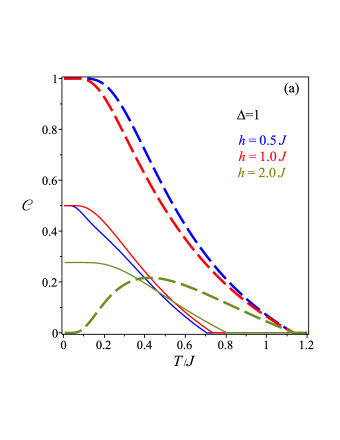
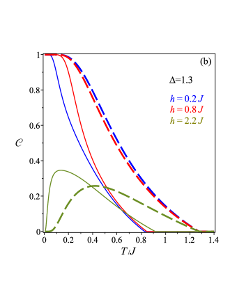
Figure 2: (Color online) The concurrence $\mathcal{C}$ as a function of $T/J$, with $J_{1}/J=1$. For the model Ising-$XXZ$ without impurities (solid curve), we have $\alpha=0$, $\gamma=0$ and $\eta=0$. With an impurity(dashed curve), we fixed $\alpha=0$, $\gamma=0.8$ and $\eta=-0.8$. (a) $\Delta=1.0$ . (b) $\Delta=1.3$.

IV.2 The $l_{1}$-norm of coherence

In order to illustrate the quantum coherence in our model, the $l_{1}$-norm $\mathcal{C}_{l_{1}}$ versus the temperature $T/J$ is plotted in Fig. 3 for different values of the magnetic field and for the anisotropic parameter $\Delta=1$ and $\Delta=1.3$, respectively. In Fig. 3(a), we observe a dramatic increase in the $l_{1}$-norm $\mathcal{C}_{l_{1}}$ for weak magnetic fields, when the impurity is included in the model. For the strong magnetic field case, $h/J=2.0$, the impurity diamond chain has a singular behavior in the quantum coherence. For low temperatures, the quantum coherence is null. Suddenly, the system increases the coherence, reaching the value $\mathcal{C}_{l_{1}}\approx 0.25$ and decreasing monotonically as soon as the $T/J$ increases. In Fig. 3(b), the results of $\mathcal{C}_{l_{1}}$ indicate that, for low temperatures, the quantum coherence is maximum, that is, $\mathcal{C}_{l_{1}}=1.0$, for both models. However, for the higher temperature, the quantum coherence with impurity is more robust for the weak magnetic field case in comparison to that without it. On the other hand, for strong magnetic fields, the quantum coherence behavior is very similar to that of the concurrence: at first, it is null and soon a sudden birth occurs until it reaches the value $\mathcal{C}_{l_{1}}\approx 0.28$. Soon after, it monotonically decreases with the increasing of the temperature. It is interesting to notice that both the concurrence and the quantum coherence have the same behavior at low temperatures, but when the temperature increases, the quantum coherence happens to predominate over the quantum entanglement(see Fig. 2 and Fig. 3).

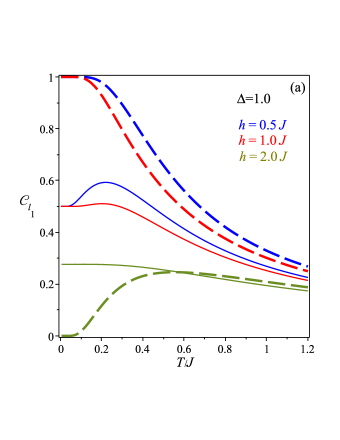
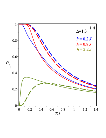
Figure 3: (Color online) The $l_{1}$-norm of coherence $\mathcal{C}_{l_{1}}$ as a function of temperature $T/J$ for $J_{1}/J=1.0$ and different values of the magnetic field $h$. (a) $\Delta=1.0$. (b) $\Delta=1.3$. The impurity parameters are set to $\alpha=0$, $\gamma=0.8$ and $\eta=-0.8$.

IV.3 Threshold temperature

We now investigated the effects of the temperature on the behavior of the thermal concurrence and on the quantum coherence with the presence of a strong external magnetic field. Figures 2 and 3 show an unusual behavior in the concurrence and in the quantum coherence ($l_{1}$-norm) for strong magnetic fields ($h/J=2.0$ and $h/J=2.2$). In Fig. 4, we display the phase diagram of the entangled region (E) and the disentagled region (D), as a function of both the anisotropy parameter $\Delta$ and the threshold temperature $T_{th}/J$ for some values of the magnetic field and the fixed value $J_{1}/J=1$. Also, we set the parameters of the impurity as $\alpha=0$, $\gamma=0.8$ and $\eta=-0.8$. Here, the threshold temperature, delimits the regime of the entangled spins (finite concurrence) and the disentangled spins (vanishing concurrence). The entangled region (E) is the entangled state in the quantum ferrimagnetic phase, which was denoted by $ENQ$, while the disentangled region (D) is the unentangled ferromagnetic state which is denoted by $UFM$ (see Ref. moi ). It is observed from Fig. 4 (a), for strong magnetic field ($h/J=2.0$), the re-entrant behavior of the thermal entanglement when the anisotropy parameter ($\Delta=1$) is sufficiently close but slightly below the ground-state boundary between the $ENQ$ and $UFM$ phases (see Ref. moi ). Under this condition, the concurrence/coherence starts from zero (see blue dashed line) in $UFM$ phase (disentangled), then it transits from the disentagled state to the entangled one in the $ENQ$ phase, that is, an increase in the temperature makes the system thermally entangled(the sudden emergence of quantum coherence) to finally return to the non-entangled $UFM$ phase. In Fig.4 (b), we display the phase diagram for both the entangled region and the disentangled one as a function of the anisotropy parameter and the threshold temperature, for a fixed value of the magnetic field $h/J=2.2$ and $\Delta=1.3$. In this figure, the green dashed line shows the transition going from the disentangled region to the entangled one, and then back to the former(D-E-D). This transition is made possible solely due to the re-entrance of the impurity bipartite entanglement.

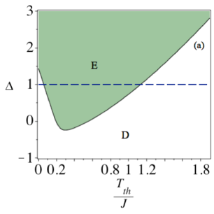
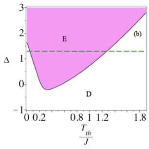
Figure 4: (Color online) The concurrence $\mathcal{C}$ depending on the anisotropy parameter and threshold temperature, when $J_{1}/J=1$ and $\alpha=0$, $\gamma=0.8$ and $\eta=-0.8$. (a) $h/J=2.0$ and $\Delta=1.0$ (blue dashed line). (b) $h/J=2.2$ and $\Delta=1.3$ (green dashed line).

V The thermal entangled teleportation

In this section, we implement teleportation throughout an entanglement mixed state; it can be regarded as a general depolarizing channel bo ; peres and we investigate the influence of the impurity of the Ising-$XXZ$ diamond chain on the quantum teleportation. We study the quantum teleportation via entangled states of a couple of impurity Heisenberg dimer in the Ising-$XXZ$ diamond chain. We consider two qubits in an arbitrary unknown state $|\psi_{in}\rangle$ as a input, that is,

$$|\psi_{in}\rangle=\cos\left(\frac{\theta}{2}\right)|10\rangle+e^{i\phi}\sin\left(\frac{\theta}{2}\right)|01\rangle\;,$$

where $0\leqslant\theta\leqslant\pi$ and $0\leqslant\phi\leqslant 2\pi$. Here, $\theta$ describes an arbitrary state and $\phi$ is the corresponding phase of this state. In the density operator formalism, the concurrence $\mathcal{C}_{in}$ of the input state, $\rho_{in}=|\psi_{in}\rangle\langle\psi_{in}|$, can be written as

$$\mathcal{C}_{in}=2|e^{i\phi}\sin\left(\frac{\theta}{2}\right)\cos\left(\frac{\theta}{2}\right)|=|\sin(\theta)|\;.$$

When the quantum state $\rho_{in}$, which is depicted in Fig. 5, is teleported via the mixed channel $\widetilde{\rho}_{ch}$, the output replica state $\widetilde{\rho}_{out}$ can be obtained by applying a joint measurement and the local unitary transformation to the input state $\rho_{in}$bo ; peres ,

$$\widetilde{\rho}_{out}=\sum_{i,j=\left\{0,x,y,z\right\}}p_{i}p_{j}\left(\sigma_{i}\otimes\sigma_{j}\right)\rho_{in}\left(\sigma_{i}\otimes\sigma_{j}\right)\;,$$

in which $p_{i}=tr\left[E^{i}\widetilde{\rho}_{ch}\right]$, $E^{0}=|\Psi^{-}\rangle\langle\Psi^{-}|$, $E^{1}=|\Phi^{-}\rangle\langle\Phi^{-}|$, $E^{2}=|\Phi^{+}\rangle\langle\Phi^{+}|$ and $E^{3}=|\Psi^{+}\rangle\langle\Psi^{+}|$, where $|\Phi^{\pm}\rangle=\frac{1}{\sqrt{2}}\left(|00\rangle\pm|11\rangle\right)$ and $|\Psi^{\pm}\rangle=\frac{1}{\sqrt{2}}\left(|01\rangle\pm|10\rangle\right)$ are Bell states. Here, we consider the density operator channel as $\widetilde{\rho}_{ch}\equiv\widetilde{\rho}(T)$.

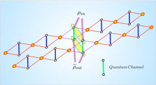
Figure 5: The schematic representation for the teleportation of the input state $\rho_{in}$, through a couple of independent impurity Heisenberg dimers (green lines) in an Ising-$XXZ$ diamond chain. The teleported output state is denoted by $\widetilde{\rho}_{out}$.

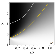
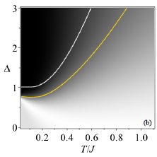
Figure 6: (Color online) The density plot of the average fidelity $F_{A}$ as a function of $\Delta$ versus $T/J$. (a) $h/J=0$. (b) $h/J=1.0$. In these figures, the yellow solid curve is the contour for $F_{A}=2/3$ in the model with impurity and white one corresponds to the model without it. The black(white) region corresponds to $F_{A}=1(0)$ and the gray regions indicate an average fidelity, $0<F_{A}<1$.

The output density operator $\widetilde{\rho}_{out}$ is described by

$$\widetilde{\rho}_{out}=\left[\begin{array}[]{cccc}c&0&0&0\\ 0&f&\Xi&0\\ 0&\Xi&g&0\\ 0&0&0&c\end{array}\right]\;.$$ (30)

The elements of the operators can be expressed as

$$\begin{array}[]{cl}c=&2\widetilde{\rho}_{2,2}\left(\widetilde{\rho}_{1,1}+\widetilde{\rho}_{4,4}\right),\\ f=&\left(\widetilde{\rho}_{1,1}+\widetilde{\rho}_{4,4}\right)^{2}\cos^{2}\left(\frac{\theta}{2}\right)+4\widetilde{\rho}_{2,2}^{\,2}\sin^{2}\left(\frac{\theta}{2}\right),\\ g=&4\widetilde{\rho}_{2,2}^{\,2}\cos^{2}\left(\frac{\theta}{2}\right)+\left(\widetilde{\rho}_{1,1}+\widetilde{\rho}_{4,4}\right)^{2}\sin^{2}\left(\frac{\theta}{2}\right),\\ \Xi=&2e^{i\phi}\widetilde{\rho}_{2,3}^{\,2}\sin\theta\;.\end{array}$$

By using the Eq. (30) in the definition of concurrence, Eq. (27), we obtain the output concurrence $\mathcal{C}_{out}(\widetilde{\rho})$ which is given by

$$\mathcal{C}_{out}(\widetilde{\rho})=2max\left\{2\widetilde{\rho}_{2,3}^{\,2}\mathcal{C}_{in}-2|\widetilde{\rho}_{2,2}||\widetilde{\rho}_{1,1}-\widetilde{\rho}_{4,4}|,0\right\}.$$

More recently, the teleportation of the same entangled state was studied in this model without any impurities moi-1 .

VI The Fidelity of entanglement teleportation

In this section, we mainly focus on how much entanglement is teleported. The fidelity between $\rho_{in}$ and $\rho_{out}$ characterizes the quality of the teleported state. The fidelity is defined by Joz ; shu

$$F=\langle\psi_{in}|\rho_{out}|\psi_{in}\rangle\;.$$

After some algebra, one finds

$$F=\frac{\sin^{2}\theta}{2}\left[\left(\widetilde{\rho}_{1,1}+\widetilde{\rho}_{4,4}\right)^{2}+4\widetilde{\rho}_{2,3}^{\,2}-4\widetilde{\rho}_{2,2}^{\,2}\right]+4\widetilde{\rho}_{2,2}^{\,2}.$$ (31)

The average fidelity $F_{A}$ of teleportation can be formulated as

$$F_{A}=\frac{1}{4\pi}\intop_{0}^{2\pi}d\phi\intop_{0}^{\pi}F\sin\theta d\theta\;.$$

According to the Eq.(31), one can get the analytic expression for $F_{A}$ as follows,

$$F_{A}=\frac{1}{3}\left[\left(\widetilde{\rho}_{1,1}+\widetilde{\rho}_{4,4}\right)^{2}+4\widetilde{\rho}_{2,3}^{\,2}-4\widetilde{\rho}_{2,2}^{\,2}\right]+4\widetilde{\rho}_{2,2}^{\,2}\;.$$ (32)

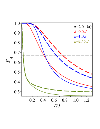
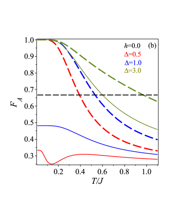
Figure 7: (Color online) The average fidelity of the teleportation $F_{A}$ is plotted against the temperature $T/J$. We consider $\alpha=0.0$, $\gamma=0.8$, $\eta=-0.8$ and $J_{1}/J=1.0$. (a) $\Delta=2.0$. (b) $h/J=0$. Horizontal dashed line indicates the $2/3$ constant line.

The average fidelity $F_{A}$ is dependent on the quantum channel parameters. In order to transmit the input state $|\psi_{in}\rangle$ with better fidelity than any classical communication protocol, $F_{A}$ must be greater than $2/3$. Taking into account the effects of an impurity on the fidelity of entanglement teleportation, we compare it with that given in the original modelmoi-1 . In Fig. 6, we illustrate the density plot of the average fidelity $F_{A}$ as a function of $T/J$ and $\Delta$, for the two fixed values of the magnetic field $h/J=0$ and $h/J=1.0$, respectively. The black region corresponds to the maximum average fidelity ($F_{A}=1$), while that the white one corresponds to $F_{A}=0$. In addition, the white (yellow) curve is used to represent the surrounding. The dark region ($F_{A}>2/3$) surrounded by curve white(yellow) indicates where the quantum teleportation will become successful, whereas the outside means that the quantum teleportation fails to be observed in the without(with) impurity case, respectively. In the Fig. 6(a), it is depicted the density plot of $F_{A}$ versus $\Delta$ and $T/J$, for the null magnetic field. As can be observe in it, a wide region where the teleportation of information is successful beyond the allowed region (limited for white curve) in the impurity free case. This means that the introduction of impurities allow the efficiency enhancement of the quantum teleportation. It is also observed that the quantum teleportation of the isotropic model ($\Delta=1$) is only possible at $T=0$, whereas in the presence of impurity it is possible for $T\geqslant 0$. In Fig. 6 (b), we have the density plot $F_{A}$ as a function of $\Delta$ and $T/J$, now for magnetic field $h/J=1.0$. In it, we also observe an enhancement in the efficiency of the average fidelity due to the inserted impurity. This increase is indicated by the region contorted by both the white and yellow curves. In addition, in order to understand the effects of the magnetic field $h/J$ and the anisotropic parameters $\Delta$ on the average fidelity, in Fig. 7, we plot $F_{A}$ as a function of the temperature $T/J$ under the conditions $\Delta=2.0$ and $h/J=0$, respectively. In Fig. 7(a), we fixed the anisotropic parameter as $\Delta=2.0$. From it, it is easy to see that they can enhance the average fidelity for weak magnetic fields. For higher magnetic fields and low temperatures the effect of the impurity on the teleportation of information does not occurs. On the other hand, in Fig. 7 (b), we fixed $h/J=0$ and we notice that for either $\Delta=0.5$ or $\Delta=1.0$, the average fidelity $F_{A}$ remains below $2/3$, making it impossible to the existence of the quantum teleportation of the information. However, when we consider the inclusion of impurity, we have a dramatic increase of such a quantity and, at low temperatures, it reaches its maximum and soon afterwards decreases monotonically as soon as the temperature increases. Taking into account the strong anisotropy ($\Delta=3.0$), the average fidelity is the same as that without impurity in low temperatures, but by increasing the temperature, we observe a clear advantage of the our model with impurity over the case without it. These results show that we can get a significant enhancement of the fidelity by the inclusion of impurities in the structure of the model.

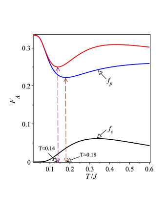
Figure 8: (Color online) The average fidelity of the teleportation $F_{A}$, $f_{p}$, $f_{c}$ as a function of the temperature $T/J$ for the original model ($\alpha=0$, $\gamma=0$, $\eta=0$) with $J_{1}/J=1.0$, $h=0$ and $\Delta=0.5$. Magenta vertical dashed line indicates the minimum of the average fidelity and the brown vertical dashed line indicate the minimum of the term $f_{p}$.

Finally, in the Fig. 7(b), the average fidelity exhibits intriguing non-monotonous temperature dependence for $\Delta=0.5$ in the classical communication region (red line). In order to understand this behavior of the average fidelity, we rewrite Eq.(32) as $F_{A}=f_{p}+f_{c}$, where

$$\begin{array}[]{cl}f_{p}=&\frac{1}{3}\left[\left(\rho_{1,1}+\rho_{4,4}\right)^{2}+8\rho_{2,2}^{\,2}\right],\\ f_{c}=&\frac{4}{3}\rho_{2,3}^{\,2}.\end{array}$$

The term $f_{p}$ is a function of the elements of the population of the density operator, while the term $f_{c}$ is a function of the quantum coherence one. In Fig. 8 , we observed the term $f_{p}$ decays to a minimum at $T/J\approx 0.18$, whereas the term $f_{c}$ is initially null from $T=0$ to $T\approx 0.05$, then it increases the quantum coherence $f_{c}$ at a rate greater than decay of therm $f_{p}$. This way, the average fidelity reaches the minimum at $T\approx 0.14$, increases until reaching a maximum and then decreases monotonically. The curves of the average fidelity show similar behavior in $0<\Delta<1$.

VII Concluding remarks

In summary, we have investigated the effects due to the inclusion of an impurity plaquette on the spin-1/2 Ising-$XXZ$ diamond chain. The concurrence and $l_{1}$-norm of the coherence is chosen as the measurement of the thermal quantum correlation and they are obtained by means of the transfer-matrix approach. We found that such a inclusion in the system can induces a significant enhancement on the thermal entanglement and on the quantum coherence. It is found that the concurrence is more robust for low magnetic field. For strong magnetic fields, we observed a sudden birth of the entanglement. Similarly, this behavior also appeared in the quantum coherence. We have also discussed the teleportation of the two-qubits in an arbitrary state through a couple of quantum channel composed by impurity Heisenberg dimers in an infinite Ising-$XXZ$ diamond chain. We observe how the teleportation of information is successful beyond the allowed region in the impurity free case. So, we showed that the average fidelity of teleportation could be enhanced for some suitable impurity parameters. The influence of the impurity is more evident in the average fidelity when we consider the null magnetic field. We saw that it is possible to teleport information in a wide range of anisotropic models. This is impossible in the model without any impurity. As a final word, we state that considerable enhancement of the teleportation can be achieved by tuning the strength of the impurity parameters. This can be used locally to control the quantum resources and the quantum teleportation of the information, unlike the original model where it is globally done.

References

• (1) A. Streltsov, H. Kampermann, S. Wolk, M. Gessner, D. Bru$\mathfrak{\beta}$, New J. Phys. 20, 053058 (2018).
• (2) A. Streltsov, G. Adesso, M. B. Plenio, Rev. Mod. Phys. 89, 041003 (2017).
• (3) C. H. Bennett, G. Brassard, C. Crepeau, C. Jozsa, A. Peres, W. K. Wootters, Phys. Rev. Lett. 70, 1895 (1993).
• (4) C. H. Bennett and D. P. Di Vincenzo, Nature 404, 247 (2000).
• (5) L. Amico, R. Fazio, A. Osterloh, V. Vedral, Rev. Mod. Phys. 80, 517 (2008).
• (6) C. Radhakrishnan, M. Parthasarathy, S. Jambulingam, T. Byrnes, Sci. Rep. 7, 13865 (2017).
• (7) G. Karpat, B. Γ‡akmak, F. Fanchini, Phys. Rev. B 90, 104431 (2014).
• (8) W. Wu, J. Xu, Phys. Lett. A 381, 239 (2017).
• (9) A. Streltsov, U. Singh, H. S. Dhar, M. N. Bera, G. Adesso, Phys. Rev. Lett. 115, 020403 (2015).
• (10) G. L. Kamta, A. F. Starace, Phys. Rev. Lett. 88, 107901 (2002); M. C. Amesen, S. Bose, V. Vedral, Phys. Rev. Lett. 87, 017901 (2001); X. G. Wang, Phys. Rev. A, 64, 012313 (2001); J. Maziero, H. C. Guzman, L. C. CΓ©leri, M. S. Sarandy, R. M. Serra, Phys. Rev. A 82, 012106 (2010); B. Γ‡akmak, G. Karpat, F. F. Fanchini, Entropy 17, 790 (2015); J. Maziero, H. Guzman, L. CΓ©leri, M. Sarandy, R. Serra, Phys. Rev A 82, 012106 (2010).
• (11) Y. Yeo, Phys Rev. A, 66, 062312 (2002); G. F. Zhang, Phys. Rev. A 75, 034304 (2007).
• (12) H. Kikuchi, Y. Fujii, M. Chiba, S. Mitsudo, T. Idehara, Physica B 329, 967 (2003).
• (13) M. Jascur, J. Strecka, J. Magn. Magn. Matter. 272, 984 (2004); O. Rojas, S. M. de Souza, V. Ohanyan, M. Khurshudyan, Phys. Rev. B 83, 094430 (2011).
• (14) O. Rojas, S. M. de Souza, V. Ohanyan, M. Khurshudyan, Phys. Rev. B 83, 094430 (2011); L. GΓ‘lisovΓ‘, Phys. Status Solidi B 250, 187 (2013); O. Rojas, S. M. de Souza, Phys. Lett. A 375, 1295 (2011).
• (15) O. Rojas, M. Rojas, N. S. Ananikian, S. M. de Souza, Phys. Rev. A 86, 042330 (2012).
• (16) W. W. Cheng, X. Y. Wang, Y. B. Sheng, L. Y. Gong, S. M. Yhao, J. M. Liu, Sci. Rep. 7, 42360 (2017).
• (17) J. Torrico, M. Rojas, S. M. de Souza, O. Rojas, N. S. Ananikian, Europhys. Lett. 108, 50007 (2014); J. Torrico, M. Rojas, M. S. S. Pereira, J. Strecka, M. L. Lyra, Phys. Rev. B 93, 014428 (2016).
• (18) O. Rojas, M. Rojas, S. M. de Souza, J. Torrico, J. Strecka, M. L. Lyra, Physica A 486, 367 (2017).
• (19) M. Rojas, S. M. de Souza, Onofre Rojas, Ann. Phys. 377, 506 (2017).
• (20) H. Falk, Phys. Rev. 151, 304 (1966); J. Stolze, M. Vogel, Phys. Rev. B 61, 4026 (2000).
• (21) T. Fukuhara, A. Kantian, M. Endres, M. Cheneau, P. Schau$\beta$, S. Hild, D. Bellem, U. Schollw$\ddot{o}$ck, T. Giamarchi, C. Gross, I. Bloch, S. Kuhr, Nature Physics 9, 235 (2013).
• (22) X. Huang, T. Si, Z. Yang, Physica B 462, 25 (2015); X. Xi, S. Hao, W. Chen, R. Yue, Phys. Lett. 297, 291 (2002); T. J. G. Apollaro, F. Plastina, L. Banchi, A. Cuccoli, R. Vaia, P. Verrucchi, M. Paternostro, Phys. Rev. A 88, 052336 (2013).
• (23) H. Fu, A. I. Solomon, X. Wang, J. Phys. A: Math. Gen. 35, 4293 (2002); W. W. Cheng, Y. X. Huang, T. K. Liu, H. Li, Physica E 39, 150 (2007); S. Li, J. Xu, Phys Lett. A 334, 109 (2005).
• (24) I. M. Carvalho, O. Rojas, S. M. de Souza, M. Rojas, Quantum Inf. Process. 18, 134 (2019).
• (25) R. J. Baxter, Exactly Solved Models in Statistical Mechanics. Academic, New York (1982).
• (26) S. Hill, W. K. Wootters, Phys. Rev. Lett. 78, 5022 (1997).
• (27) W. K. Wootters, Phys. Rev. Lett. 80, 2245 (1998).
• (28) T. Baumgratz, M. Cramer, M. B. Plenio, Phys. Rev. Lett. 113, 140401 (2014).
• (29) G. Bowen, S. Bose, Phys. Rev. Lett. 87, 267901 (2001).
• (30) A. Peres, Phys. Rev. Lett. 77, 1413 (1996).
• (31) R. Jozsa, J. Mod. Opt. 41, 2315 (1994).
• (32) B. Shumacher, Phys. Rev. A 54, 2614 (1996).