Rotating and non-rotating AdS black holes in $f({\mathcal{T}})$ gravity non-linear electrodynamics

Abstract

We derive new exact charged $d$-dimensional black hole solutions for quadratic teleparallel equivalent gravity, $f({\mathcal{T}})=a_{0}+a_{1}{\mathcal{T}}+a_{2}{\mathcal{T}}^{2}$, where $\mathcal{T}$ is the torsion scalar, in the case of non-linear electrodynamics. We give a specific form of electromagnetic function and find out the form of the unknown functions that characterize the vielbeins in presence of the electromagnetic field. It is possible to show that the black holes behave asymptotically as AdS solutions and contain, in addition to the monopole and quadrupole terms, other higher order terms whose source is the non-linear electrodynamics field. We calculate the electromagnetic Maxwell field and show that our d-dimensional black hole solutions coincide with the previous obtained one Awad et al. (2017). The structure of the solutions show that there is a central singularity that is much mild in comparison with the respective one in General Relativity. Finally, the thermodynamical properties of the solutions are investigated by calculating the entropy, the Hawking temperature, the heat capacity, and other physical quantities. The most important result of thermodynamics is that the entropy is not proportional to the area of the black hole. This inanition points out that we must have a constrain on the quadrupole term to get a positive entropy otherwise we get a negative value.

I Introduction

Understanding of the gravitational interaction at large scales is considered a main issue of theoretical physics and cosmology Farrugia et al. (2016). For example, Einstein’s General Relativity (GR) is not able to explain the accelerated expansion epoch of our universe Riess et al. (1998); Perlmutter et al. (1999); Hinshaw et al. (2013); Eisenstein et al. (2005); Wang (2008). This issue can be solved in the framework of GR if some cosmic flow, having exotic properties, is assumed, the so-called dark energy, or a cosmological constant is involved into the field equation Peebles and Ratra (2003). Moreover, the rotation curves of spiral galaxy are out the domain of validity of GR unless one assumes the existence of cold and pressureless dark matter Binney and Tremaine (1987).

Despite of this state of art, GR has achieved brilliant successes in many aspects like solar system dynamics, gravitational wave detection, relativistic stellar structure up to cosmology Will (2014). Einstein’s GR has a question mark when it is confronted with large scales or when quantization is taken into account. Therefore, there is the necessity for a self-consistent theory that is capable of describing the gravitational interaction ranging from quantum to cosmic scales and coinciding with GR in the limits where it is successful.

According to this philosophy, there are several proposals to extend or modify GR in view of obtaining a self-consistent theory at any scale. The so called $f(R)$ gravity is one of these proposal. Here $R$ is the Ricci scalar and, for $f(R)=R$, its Lagrangian corresponds to the Hilbert-Einstein Lagrangian and GR is recovered Capozziello and Francaviglia (2008). In some sense, $f(R)$ gravity is the minimal extension of GR. Another proposal is $f({\mathcal{T}})$ gravity in which ${\mathcal{T}}$ represents torsion scalar. Also in this case, for $f({\mathcal{T}})={\mathcal{T}}$, the theory reduces to the so called Teleparallel Equivalent General Relativity (TEGR) which is constructed by the Weitzenböck geometry and it is endowed with a nonsymmetric connection, characterized by no curvature and non-vanishing torsion de Andrade et al. (2000); Nashed (2018); Aldrovandi et al. (2003); Maluf (2013). The TEGR torsion tensor plays the dynamical role of curvature and the vielbein plays the role of metric tensor, that is the gravitational potentials. Einstein used TEGR theory to construct a unification between gravitational and electromagnetism fields Unzicker and Case (2005); Nashed (2003); de Andrade and Pereira (1997); Maluf (2013). Although, TEGR is constructed using a different geometry from that of GR based on Riemann geometry, that is the Weitzenböck geometry, TEGR and GR are completely equivalent from a dynamical point of view. However, assuming generic functions $f(R)$ and $f(\mathcal{T})$, they are inequivalent Mai and Lü (2017); Ferraro and Fiorini (2008); Fiorini and Ferraro (2009). Therefore, those theories are interesting and can be considered to solve the problems of dark energy and dark matter Cardone et al. (2012); Myrzakulov (2011); Nashed and El Hanafy (2017); Yang (2011); Bengochea (2011); Bamba et al. (2010); Karami and Abdolmaleki (2013); Dent et al. (2011); Cai et al. (2011); Capozziello et al. (2011); Bamba et al. (2013); Camera et al. (2014); Nashed (2015, 2013a); Shirafuji et al. (1996). In this study, we are considering $f({\mathcal{T}})$ gravitational theories.

There are many applications of $f({\mathcal{T}})$ in solar system as well as in cosmological frame. For example, exact solutions, black hole solutions and stellar models are discussed in Wang (2011); Ferraro and Fiorini (2011); Nashed et al. (2019); Iorio et al. (2015); Nashed and Capozziello (2018); Awad et al. (2018); González et al. (2012); Awad et al. (2019); Hanafy and Nashed (2017); Iorio et al. (2016); Junior et al. (2015, 2015, 2015); Awad et al. (2018); Harko et al. (2014); Capozziello et al. (2013); Rodrigues et al. (2013); Nashed (2013b, 2010); Junior et al. (2015); Bejarano et al. (2015). Spherically symmetric solutions with constant torsion scalar have been derived in Gamal (2012); Nashed (2014). In the solar system, it is possible to obtain a weak field solution Iorio and Saridakis (2012) for the form $f({\mathcal{T}})={\mathcal{T}}+\alpha{\mathcal{T}}^{2}$ for which the authors constrain the dimensional parameter $\alpha$ Xie and Deng (2013). $f({\mathcal{T}})$ has extra degrees of freedom which are related to the non-invariance of the theory under local Lorentz transformations. Recently, an invariant $f({\mathcal{T}})$ gravitational theory under local Lorentz transformation has been derived Tamanini and Böhmer (2012). In the frames of cosmology and spherically symmetric geometry, it is shown that the diagonal ansatz is not a suitable vielbein to be used Ruggiero and Radicella (2015). A non diagonal spherically symmetric vielbein has been applied to the field equations of $f({\mathcal{T}})$ gravity and a weak field solution has been obtained Iorio et al. (2015). Recently, new charged black holes for quadratic and cubic form of $f({\mathcal{T}})$ have been derived using flat horizons spacetimes Awad et al. (2017); Nashed and Saridakis (2019). It is the purpose of the present paper to study the effect of the non-linear electrodynamics in $f({\mathcal{T}})$ gravity on a cylindrical spacetime. This approach could have interesting physical applications both for gravitational and electromagnetic fields.

The layout of the paper is the following: In Section II we summarize $f({\mathcal{T}})$ gravity and derive the field equations in presence of non-linear electrodynamics. In Section III we derive charged static AdS solutions, analyzing the structure of singularities. In Section IV we obtain charged rotating AdS solution in non-linear electrodynamics in the context of $f({\mathcal{T}})$ gravity. Section V is devoted to thermodynamics considering entropy, Hawking temperature, heat capacity, Gibbs free energy. The most interesting feature of these calculations is the fact that the entropy is not proportional to the area of the black hole in addition to the possibility of negative values of entropy. Section VI is devoted to discussion and conclusions.

II Basic concepts of $f({\mathcal{T}})$ gravity

In Riemannian geometry, the metric of the spacetime has the form

$$ds^{2}:=g_{\mu\nu}dx^{\mu}dx^{\nu},$$ (1)

where $g_{\mu\nu}$ is a second order symmetric tensor. Using the vielbein one can write Eq. (1) as

$$ds^{2}:=g_{\mu\nu}dx^{\mu}dx^{\nu}=\eta_{ij}\vartheta^{i}\vartheta^{j},\quad\textrm{where}\quad\vartheta^{i}={h^{i}}_{\mu}dx^{\mu},$$ (2)

with $\eta_{ij}$ being the Minkowskian metric that is defined as: $\eta_{ij}=diag(-1,+1,+1,\cdots,+1)$ and ${h^{i}}_{\mu}$ is the covariant vielbein that satisfies the orthogonality conditions

$${h^{i}}_{\mu}{h_{j}}^{\mu}={\delta_{j}}^{i},\qquad\qquad{h^{i}}_{\mu}{h_{i}}^{\nu}={\delta_{\mu}}^{\nu}.$$ (3)

To construct a spacetime with vanishing curvature and a non-vanishing torsion one has to define the Weitzenböck connection which is

$${\Gamma^{\lambda}}_{\nu\mu}={h_{i}}^{\lambda}~{}\partial_{\mu}h^{i}{{}_{\nu}}=-h^{i}{{}_{\nu}}\partial_{\mu}{h_{i}}^{\lambda},\qquad\textrm{where}\qquad\partial_{\mu}=\frac{\partial}{\partial x^{\mu}}.$$ (4)

Using Eq. (4), the torsion and contorsion tensors are

$${T^{\alpha}}_{\mu\nu}:={\Gamma^{\alpha}}_{\nu\mu}-{\Gamma^{\alpha}}_{\mu\nu},\qquad\qquad{\gamma^{\mu\nu}}_{\alpha}:=-\frac{1}{2}\left({T^{\mu\nu}}_{\alpha}-{T^{\nu\mu}}_{\alpha}-{T_{\alpha}}^{\mu\nu}\right).$$ (5)

From Eqs. (5), one can define the superpotential tensor

$${S^{\lambda\mu}}_{\nu}=\frac{1}{2}\left({\gamma^{\mu\nu}}_{\alpha}+\delta^{\mu}_{\alpha}{T^{\beta\nu}}_{\beta}-\delta^{\nu}_{\alpha}{T^{\beta\mu}}_{\beta}\right).$$ (6)

From Eqs. (5) and (6) the torsion scalar is provided as

$${\mathcal{T}}:={T^{\alpha}}_{\mu\nu}{S_{\alpha}}^{\mu\nu}.$$ (7)

The Lagrangian of TEGR theory is constructed from the torsion scalar given by Eq. (7).

Let us now consider $f({\mathcal{T}})$ gravity minimally coupled with non-linear electrodynamics. Thence, the action of this theory is given by

$${\mathcal{L}}:=\frac{1}{2\kappa}\int|h|f({\mathcal{T}})~{}d^{d}x+\int|h|{\mathcal{L}({\mathcal{F}})}~{}d^{d}x,$$ (8)

with $|h|=\sqrt{-g}=\det\left({h^{a}}_{\mu}\right)$ being the determinant of the metric and $\kappa$ a dimensional constant with the form $\kappa=2(d-3)\Omega_{d-1}G_{d}$, with $G_{d}$ being the Newtonian gravitational constant in $d$-dimensions and $\Omega_{d-1}$ a $(d-1)$-dimensional unitary volume whit the form

$$\Omega_{d-1}=\frac{2\pi^{(d-1)/2}}{\Gamma((d-1)/2)},$$ (9)

where $\Gamma$ is the $\Gamma$-function (when $d=4$, it is $2(d-3)\Omega_{d1}=8\pi$). The electromagnetic Lagrangian ${\mathcal{L}({\mathcal{F}})}$ is gauge-invariant and depends on the invariant ${\mathcal{F}}$ defined as ${\mathcal{F}}=\frac{1}{4}{\mathcal{F}}_{\alpha\beta}{\mathcal{F}}^{\alpha\beta}$ Plebański (1970). The antisymmetric Faraday tensor is defined as

$${\mathcal{F}}_{\alpha\beta}={\mathcal{E}}_{\alpha,\beta}-{\mathcal{E}}_{\beta,\alpha},$$ (10)

where ${\mathcal{E}}_{\mu}$ is its gauge potential 1-form. In the Maxwell theory, the Lagrangian ${\mathcal{L}({\mathcal{F}})}$ is ${\mathcal{L}({\mathcal{F}})}=4\mathcal{F}$. Here, we consider a more general choice of the electromagnetic Lagrangian. From Action (8), the non-linear electrodynamics is described by nonlinear terms in ${\mathcal{F}}_{\alpha\beta}$ and its invariants. However, we can provide a dual representation in terms of an auxiliary field ${\mathcal{P}}_{\alpha\beta}$ . This method is proved to be highly benefit to derive exact solutions in GR, specifically for the electric case Ayon-Beato (1999); Salazar I. et al. (1987). The dual form can be obtained adopting the Legendre transformation below:

$${\mathcal{\aleph}}=2{\mathcal{F}}{\mathcal{L}}_{\mathcal{F}}-{\mathcal{L}},\quad\textrm{where}\qquad{\mathcal{L}}_{\mathcal{F}}=\frac{\partial{\mathcal{L}}}{\partial{\mathcal{F}}},$$ (11)

where ${\mathcal{\aleph}}$ is an arbitrary function depending on the invariant ${\mathcal{P}}$, defined as ${\mathcal{P}}=\frac{1}{4}{\mathcal{P}}_{\alpha\beta}{\mathcal{P}}^{\alpha\beta}$. From Eq. (11), non-linear electrodynamics can be recast in terms of ${\mathcal{P}}$ according to the formulas

$${\mathcal{P}}_{\mu\nu}={\mathcal{L}}_{\mathcal{F}}{\mathcal{F}}_{\mu\nu},\qquad\qquad{\mathcal{F}}_{\mu\nu}={\mathcal{\aleph}}_{\mathcal{P}}{\mathcal{P}}_{\mu\nu},\qquad\qquad{\mathcal{L}}=2{\mathcal{P}}{\mathcal{\aleph}}_{\mathcal{P}}-{\mathcal{\aleph}},$$ (12)

where the standard Maxwell theory is obtained for ${\mathcal{L}}_{F}=1$. As it is clear from the above equations, ${\mathcal{\aleph}}$ is a function of ${\mathcal{P}}$, where Ayon-Beato (1999); Salazar I. et al. (1987)

$${\mathcal{\aleph}}_{\mathcal{P}}=\frac{\partial{\mathcal{\aleph}}}{\partial{\mathcal{P}}}.$$

The variation of Lagrangian (8) with respect to the vielbeins leads to

$$\zeta^{\nu}{}_{\mu}={S_{\mu}}^{\rho\nu}\partial_{\rho}{\mathcal{T}}f_{\mathcal{T}T}+\left[h^{-1}{h^{i}}_{\mu}\partial_{\rho}\left(h{h_{i}}^{\alpha}{S_{\alpha}}^{\rho\nu}\right)-{T^{\alpha}}_{\lambda\mu}{S_{\alpha}}^{\nu\lambda}\right]f_{\mathcal{T}}-\frac{f}{4}\delta^{\nu}_{\mu}+\frac{1}{2}\kappa{{{\mathfrak{T}}^{{}^{{}^{{\!\!\!\!\scriptstyle{nlem}}}}}}}^{\nu}_{\mu}\equiv 0,$$ (13)

and the Maxwell equations for non-linear electrodynamics become Ayon-Beato (1999)

$$\partial_{\nu}\left(\sqrt{-g}{\mathcal{P}}^{\mu\nu}\right)=0.$$ (14)

The stress-energy tensor of non-linear electrodynamic is

$${{{\mathfrak{T}}^{{}^{{}^{{\!\!\!\!\scriptstyle{nlem}}}}}}}^{\nu}_{\mu}:=2({\mathcal{\aleph}}_{\mathcal{P}}{\mathcal{P}}_{\mu\alpha}{\mathcal{P}}^{\nu\alpha}-\delta_{\mu}^{\nu}[2{\mathcal{P}}{\mathcal{\aleph}}_{\mathcal{P}}-{\mathcal{\aleph}}]).$$ (15)

It is worth saying that Eq. (15) has a non-vanishing trace unlike the stress-energy tensor coincides with the Maxwell one. It is worth noticing that the electric field of linear electrodynamics is obtained as

$${\mathcal{E}}={\mathcal{F}}_{tr}={\mathcal{\aleph}}_{\mathcal{P}}{\mathcal{P}}_{tr}.$$ (16)

In this context, black hole solutions can be found.

III Anti-de-Sitter black hole solutions in non-linear electrodynamics

Let us search now for charged AdS black hole solutions in non-linear electrodynamics assuming, in general, $d$-dimensions in the framework of $f({\mathcal{T}})$ gravity. Using the following vierbein diagonal ansatz in $d$-dimensions ($t$, $r$, $\eta_{1}$, $\eta_{2}$, $\cdots$, $\eta_{n}$, $\xi_{1}$, $\xi_{2}$ $\cdots$ $\xi_{l}$), with $l=1,2\cdots$ $d-n-2$, in which $0\leq r<\infty$, $-\infty<t<\infty$, $0\leq\eta_{n}<2\pi$ and $-\infty<\xi_{k}<\infty$, we assume the vielbein Capozziello et al. (2013); Nashed and Saridakis (2019):

$$\left({h^{i}}_{\mu}\right)=\left(\sqrt{A(r)},\;\frac{1}{\sqrt{A(r)g(r)}},\;r,\;r,\;r\;\cdots\right)$$,

(17)

which corresponds to the metric

$$ds^{2}=-A(r)dt^{2}+\frac{1}{A(r)g(r)}dr^{2}+r^{2}\left(\sum_{i=1}^{n}d\eta^{2}_{i}+\sum_{l=1}^{d-n-2}d\xi_{l}^{2}\right),$$ (18)

where $A(r)$ and $g(r)$ are functions depending only on the radial coordinate $r$. Substituting the vielbein (17) into the torsion scalar in (7), we get

$${\mathcal{T}}=(d-2)\frac{A^{\prime}g}{r}+(d-2)(d-3)\frac{Ag}{r^{2}},$$ (19)

where $A^{\prime}(r)\equiv\frac{dA(r)}{dr}$ and $g^{\prime}(r)\equiv\displaystyle\frac{dg(r)}{dr}$. Finally, since the $f({\mathcal{T}})$ power law gravity seems the model with the best agreement with observational data Nesseris et al. (2013); Nunes et al. (2016); Basilakos et al. (2018), we will focus on the choice

$$f({\mathcal{T}})=a_{0}+a_{1}{\mathcal{T}}+a_{2}{\mathcal{T}}^{2},$$ (20)

where $a_{0}$, $a_{1}$ and $a_{2}$ are the model parameters.

III.1 Asymptotically static AdS black holes

Inserting the vielbein (17) into field Eqs. (13) and (14), we obtain the following non-vanishing components:

$$\zeta^{r}{}_{r}=2{\mathcal{T}}f_{\mathcal{T}}+2a_{0}-f-4\aleph=0,$$

$$\zeta^{\eta_{1}}{}_{\eta_{1}}=\zeta^{\eta_{2}}{}_{\eta_{2}}=\cdots\cdots=\zeta^{\eta_{n}}{}_{\eta_{n}}=\zeta^{\xi_{1}}{}_{\xi_{1}}=\zeta^{\xi_{2}}{}_{\xi_{2}}=\cdots\cdots=\zeta^{\xi_{d-n-2}}{}_{zeta_{d-n-2}}$$

$$=\frac{f_{{\mathcal{T}T}}[r^{2}{\mathcal{T}}+(d-3)A]{\mathcal{T}}^{\prime}}{r}+\frac{f_{\mathcal{T}}}{2r^{2}}\Biggl{\{}2r^{2}gA^{\prime\prime}+rg^{\prime}(2(d-3)A+rA^{\prime})+g(2(d-3)^{2}A+(3d-8)rA^{\prime})\Biggr{\}}-f+2a_{0}-4\aleph$$

$$+\frac{8q^{\prime}g\aleph^{\prime}}{q^{\prime}g^{\prime}+2gq^{\prime\prime}}=0,$$

$$\zeta^{t}{}_{t}=\frac{2(d-2)Agf_{{\mathcal{T}T}}{\mathcal{T}}^{\prime}}{r}+\frac{(d-2)f_{\mathcal{T}}}{r^{2}}\Biggl{\{}2[(d-3)Ag+rgA^{\prime}]+rAg^{\prime}\Biggr{\}}-f-4\aleph+2a_{0}=0,$$

where $q(r)\equiv q$ is the gauge 1-form of the non-linear electrodynamics that is defined as ${\mathcal{P}}_{tr}=q^{\prime}$ and $q^{\prime}=\frac{dq}{dr}$, $q^{\prime\prime}=\frac{d^{2}q}{dr^{2}}$. In the case of $f({\mathcal{T}})$ with the form given by (20), the above equations reduce to

$$\zeta^{r}{}_{r}=a_{1}{\mathcal{T}}+3a_{2}{\mathcal{T}}^{2}+a_{0}-4\aleph=0,$$ (22)

$$\zeta^{\eta_{1}}{}_{\eta_{1}}=\zeta^{\eta_{2}}{}_{\eta_{2}}=\cdots\cdots=\zeta^{\eta_{n}}{}_{\eta_{n}}=\zeta^{\xi_{1}}{}_{\xi_{1}}=\zeta^{\xi_{2}}{}_{\xi_{2}}=\cdots\cdots=\zeta^{\xi_{d-n-2}}{}_{\xi_{d-n-2}}$$

$$=\frac{2a_{2}[r^{2}{\mathcal{T}}+(d-3)A]{\mathcal{T}}^{\prime}}{r}+\frac{(a_{1}+2a_{2}{\mathcal{T}})}{2r^{2}}\Biggl{\{}2r^{2}gA^{\prime\prime}+rg^{\prime}(2(d-3)A+rA^{\prime})+g(2(d-3)^{2}A+(3d-8)rA^{\prime})\Biggr{\}}$$

$$-a_{1}{\mathcal{T}}-a_{2}{\mathcal{T}}^{2}+a_{0}-4\aleph+\frac{8q^{\prime}g\aleph^{\prime}}{q^{\prime}g^{\prime}+2gq^{\prime\prime}}=0,$$ (23)

$$\zeta^{t}{}_{t}=\frac{4a_{2}(d-2)Ag{\mathcal{T}}^{\prime}}{r^{2}}+\frac{(a_{1}+2a_{2}{\mathcal{T}})(d-2)}{r}\Biggl{\{}2[(d-3)Ag+rgA^{\prime}]+rAg^{\prime}\Biggr{\}}-{\mathcal{T}}-a_{2}{\mathcal{T}}^{2}-4\aleph+a_{0}=0,$$ (24)

where ${\mathcal{T}}^{\prime}\equiv d{\mathcal{T}}(r)/dr$ is calculated through (19).

We have to note that Eq. (22) is a second-order algebraic equation and it gives ${\mathcal{T}}={\mathcal{T}}_{0}=const$. On the other hand, Eq. (19) for ${\mathcal{T}}$ gives the solution

$$A(r)=\Lambda_{eff}r^{2}-\frac{m}{r^{d-3}},$$

where $m$ is a constant related to the mass, and the function $g(r)$ is obtained by (III.1) into (III.1). Eq. (24) gives

$$g(r)=q(r)=c\;,$$

$$\aleph(r)=\frac{a_{1}T_{0}+3a_{2}T_{0}{}^{2}+a_{0}}{4}\;.$$ (26)

In the above expressions the constant $\Lambda_{eff}$, is given by

$$\Lambda_{eff}=\frac{T_{0}}{3c}.$$ (27)

It is straightforward to see that this is an effective cosmological constant given by the torsion scalar.

The horizons of solution (III.1) is given by

$$m=\Lambda_{eff}r^{d-1},$$ (28)

which, in 4-dimensions, gives $m=\Lambda_{eff}r^{3}$.

Let us continue our analysis for the general case where the torsion scalar has non-trivial values. For a non-constant torsion scalar, we get the following solution:

$$A(r)=\frac{1}{r^{d-3}}\Big{(}\int\Big{[}r^{4(d-2)}q^{\prime 3}c_{2}-\frac{a_{1}r^{3(d-2)}q^{\prime 2}}{2a_{2}(d-2)c_{1}}\Big{]}dr+c_{3}\Big{)},$$

$$\aleph(r)=\frac{1}{16a_{2}}[a_{1}{}^{2}-4a_{0}a_{2}-8(d-2)r^{d-2}q^{\prime}a_{1}a_{2}c_{1}c_{2}+12(d-2)^{2}r^{2(d-2)}q^{\prime 2}a_{2}{}^{2}c_{1}{}^{2}c_{2}{}^{2}],$$

$$g(r)=\frac{c_{1}}{q^{\prime 2}r^{2(d-2)}},\qquad q(r)=q(r),$$ (29)

where $c_{i}$, $i=1\cdots 3$ are integration constants. We can assume a given form for the arbitrary function $\aleph(r)$ and calculate the other functions from it. So let us fix the arbitrary function to have the form

$$\aleph(r)=-\frac{Psech^{2}(\frac{q_{1}}{(d-3)mr^{d-3}})}{r^{2(d-2)}}.$$ (30)

It is worth noticing that, in case $d=4$, Eq. (30) is identical to that given in Ayon-Beato (1999). Using Eq. (30) in (III.1) we get

$$A(r)=-\frac{1}{r^{d-3}}\Big{\{}\int\frac{1}{216(d-2)^{3}r^{2(d-2)}a_{2}{}^{3}c_{1}{}^{3}c_{2}{}^{2}(1+e^{\frac{2q_{1}}{(d-3)mr^{d-3}}})^{3}}\Big{[}2a_{1}r^{d-2}[e^{\frac{2q_{1}}{(d-3)mr^{d-3}}}+1]$$

$$-\sqrt{\mathfrak{N}r^{2(d-2)}e^{\frac{4q_{1}}{(d-3)mr^{d-3}}}+2[\mathfrak{N}r^{2(d-2)}-96Pa_{2}]e^{\frac{2q_{1}}{(d-3)mr^{d-3}}}+\mathfrak{N}r^{2(d-2)}}\Big{]}^{2}\Big{[}a_{1}r^{d-2}[e^{\frac{2q_{1}}{(d-3)mr^{d-3}}}+1]$$

$$+\sqrt{\mathfrak{N}r^{2(d-2)}e^{\frac{4q_{1}}{(d-3)mr^{d-3}}}+2[\mathfrak{N}r^{2(d-2)}-96Pa_{2}]e^{\frac{2q_{1}}{(d-3)mr^{d-3}}}+\mathfrak{N}r^{2(d-2)}}\Big{]}dr+c_{3}\Big{\}},$$

$$g(r)=\frac{36(d-2)^{2}a_{2}{}^{2}r^{2(d-2)}c_{1}{}^{3}c_{2}{}^{2}(1+e^{\frac{2q_{1}}{(d-3)mr^{d-3}}})^{2}}{[2a_{1}r^{(d-2)}[e^{\frac{2q_{1}}{(d-3)mr^{d-3}}}+1]-\sqrt{\mathfrak{N}r^{2(d-2)}e^{\frac{4q_{1}}{(d-3)mr^{d-3}}}+2[\mathfrak{N}r^{2(d-2)}-96Pa_{2}]e^{\frac{2q_{1}}{(d-3)mr^{d-3}}}+\mathfrak{N}r^{2(d-2)}}]^{2}},$$

$$q(r)=\int\frac{2a_{1}r^{d-2}[e^{\frac{2q_{1}}{(d-3)mr^{d-3}}}+1]-\sqrt{\mathfrak{N}r^{2(d-2)}e^{\frac{4q_{1}}{(d-3)mr^{d-3}}}+2[\mathfrak{N}r^{2(d-2)}-96Pa_{2}]e^{\frac{2q_{1}}{(d-3)mr^{d-3}}}+\mathfrak{N}r^{2(d-2)}}}{6(d-2)r^{2(d-2)}a_{2}c_{1}c_{2}(1+e^{\frac{2q_{1}}{(d-3)mr^{d-3}}})}dr+c_{3},$$

where $\mathfrak{N}=(a_{1}{}^{2}+12a_{0}a_{2})$.

Now if we assume the constraint $\mathfrak{N}=0$, i.e., ${\displaystyle a_{0}=-\frac{a_{1}{}^{2}}{12a_{2}}}$, in Eq. (22) we get the same solution given by Eq. (III.1) except the arbitrary function $\aleph(r)$ which takes the form

$$\aleph(r)=\frac{(a_{1}-3(d-2)r^{(d-2)}q^{\prime}a_{2}c_{1}c_{2})^{2}}{12a_{2}}.$$ (32)

Considering the function (30) in (32), we get

$$A(r)=\Lambda_{eff}r^{2}-\frac{4(d-3)^{2}mq^{2}P}{(d-2)a_{1}{}^{2}c_{1}r^{d-2}q_{1}{}^{2}[e^{\frac{2q_{1}}{(d-3)mr^{d-3}}}+1]^{2}}\Big{(}2\sqrt{3P|a_{2}|}e^{\frac{q_{1}}{(d-3)mr^{d-3}}}[q_{1}\{e^{\frac{2q_{1}}{(d-3)mr^{d-3}}}-1\}+[1+e^{\frac{2q_{1}}{(d-3)mr^{d-3}}}](d-2)mr^{d-3})]$$

$$+3a_{1}q_{1}r^{d-2}[e^{\frac{2q_{1}}{(d-3)mr^{d-3}}}+1]\Big{)}+\frac{q^{2}}{(d-2)a_{1}{}^{2}c_{1}}\int\frac{8(d-3)^{2}P\sqrt{3P|a_{2}|}(q_{1}{}^{2}-(d-2)m^{2}r^{2(d-3)})e^{\frac{q_{1}}{(d-3)mr^{d-3}}}}{q_{1}{}^{2}r^{2(d-2)}[e^{\frac{2q_{1}}{(d-3)mr^{d-3}}}+1]}dr+\frac{c_{3}}{r^{d-3}},$$

$$\approx\Lambda_{eff}r^{2}-\frac{M}{r^{d-3}}+\frac{Q^{2}}{r^{2(d-3)}}+\frac{Q_{1}{}^{4}}{r^{(3d-8)}}+\frac{Q_{2}{}^{4}}{r^{4(d-3)}}+\cdots,$$

$$g(r)=\frac{a_{1}{}^{2}c_{1}r^{2(d-2)}[e^{\frac{2q_{1}}{(d-3)mr^{d-3}}}+1]^{2}}{q^{2}(d-3)^{2}\{a_{1}r^{d-2}[e^{\frac{2q_{1}}{(d-3)mr^{d-3}}}+1]-4\sqrt{3P|a_{2}|}e^{\frac{q_{1}}{(d-3)mr^{d-3}}}\}^{2}}$$

$$\approx\frac{c_{1}}{(d-3)^{2}q^{2}}\Big{[}1+\frac{4(d-3)^{2}\sqrt{3P|a_{2}|}}{a_{1}r^{d-2}}-\frac{2q_{1}{}^{2}\sqrt{3P|a_{2}|}}{a_{1}(d-3)^{2}m^{2}r^{3d-8}}-\frac{36Pa_{2}}{a_{1}{}^{2}r^{2(d-2)}}+\cdots,$$ (33)

$$q(r)=\int\frac{a_{1}r^{d-2}[e^{\frac{2q_{1}}{(d-3)mr^{d-3}}}+1]-4e^{\frac{q_{1}}{(d-3)mr^{d-3}}}\sqrt{3P|a_{2}|}}{3(d-2)r^{2(d-2)}a_{2}c_{1}c_{2}(1+e^{\frac{2q_{1}}{(d-3)mr^{d-3}}})}dr+c_{3}$$

$$\approx c_{3}+\frac{q}{r^{d-3}}-\frac{2(d-3)\sqrt{3|a_{2}|P}q}{a_{1}(2d-5)r^{2d-5}}+\frac{\sqrt{3|a_{2}|P}qq_{1}{}^{2}}{(d-3)(4d-11)a_{1}m^{2}r^{4d-11}}+\cdots,$$

where $\Lambda=-\frac{a_{1}{}^{3}}{54(d-1)(d-2)^{3}a_{2}{}^{3}c_{1}{}^{3}c_{2}{}^{2}}$, $q=-\frac{a_{1}}{3(d-2)(d-3)a_{2}c_{1}c_{2}}$, $M=c_{3}-\frac{6(d-3)^{2}Pq^{2}}{q_{1}a_{1}c_{1}(d-2)}$, $Q^{2}=\frac{6(d-3)Pq^{2}}{a_{1}c_{1}(d-2)}$, $Q_{1}{}^{4}=-\frac{8(d-3)^{2}Pq^{2}\sqrt{3P|a_{2}|}}{c_{1}(d-2)(2d-5)}$ and $Q_{2}{}^{4}=-\frac{2Pq_{1}{}^{2}q^{2}}{m^{2}a_{1}c_{1}(d-2)(d-3)}$. Using Eq. (16) we get the linear electrodynamics in the following form

$${\mathcal{E}}(r)=\frac{\phi}{r^{d-3}}+\frac{6\phi^{2}(d-2)(d-3)^{2}\sqrt{3|a_{2}|P}}{a_{1}r^{(2d-5)}(2d-5)}+\frac{q_{1}{}^{2}\phi^{2}(2d-5)}{m^{2}r^{3(d-3)}(d-3)}+\cdots,$$ (34)

where $\phi=-\frac{1}{3(d-2)(d-3)}$. To get this result, we have put $2a_{2}c_{1}{}^{2}c_{2}=a_{1}{\mathcal{P}}$. It is interesting to note that Eq. (34) coincides with that given in Awad et al. (2017) for $q_{1}=0$. The parameter $q_{1}$ is responsible for deviations from linear electrodynamics as Eq. (30) indicates. It is straightforward to show that, from (30) for $q_{1}=0$, we return to Maxwell electrodynamics and, for $q_{1}\neq 0$, we have non-linear electrodynamics. Explicitly, the effect of parameter $q_{1}$ appears in Eq. (34) showing that the gauge potential is different from the one presented in Awad et al. (2017).

If we calculate the invariants of the black hole solution (III.1), we get the same asymptotic behavior presented in Awad et al. (2017); Nashed and Saridakis (2019). These invariants show that there is a singularity at $r=0$. Approaching to $r=0$, these invariants assume the form $(K,R_{\mu\nu}R^{\mu\nu})\sim\sqrt[3]{r^{-4(d-2)}}$, and $(R,{\mathcal{T}})\sim\sqrt[3]{r^{-2(d-2)}}$, differently to the black holes of Maxwell electrodynamics in either GR or TEGR theories which have the forms $(K,R_{\mu\nu}R^{\mu\nu})\sim r^{-2d}$ and $(R,{\mathcal{T}})\sim r^{-d}$, respectively. The above results indicate in a clear way that the singularity of the non-linear charged black hole is milder than the one emerging in GR and TEGR for the charged case.

Finally, if we calculate the energy of solution (III.1) we get the same formula presented in Awad et al. (2017); Nashed and Saridakis (2019) up to the leading order, i.e. $E=\frac{(d-2)M}{4(d-3)G_{d}}$.In other words, this feature assures the consistency of the solution.

IV Rotating black holes in Maxwell-$f(T)$ gravity

Let us derive now rotating black hole solutions satisfying the field equations of the above (20) $f({\mathcal{T}})$ gravity. We start assuming the above static solution as a constraint. Taking into account the following transformations :

$$\bar{\eta}_{i}=-\Xi~{}{\eta_{i}}+\frac{n_{i}}{l^{2}}~{}t,\qquad\qquad\qquad\bar{t}=\Xi~{}t-\sum\limits_{i=1}^{\omega}n_{i}~{}\eta_{i},$$ (35)

with $n_{i}$ are rotation parameters (their number is $\omega=\lfloor(d-1)/2\rfloor$ where $\lfloor...\rfloor$ marks the integer part), and where we can define a parameter $\lambda$ connected to the $\Lambda_{eff}$ of the static solution through

$$\lambda=-\frac{(d-2)(d-1)}{2\Lambda_{eff}}.$$ (36)

Additionally, $\Xi$ is defined as

$$\Xi:=\sqrt{1-\sum\limits_{j=1}^{{\omega}}\frac{n_{j}{}^{2}}{\lambda^{2}}}.$$ (37)

Adopting the transformations (35) to the (17), we obtain

$$\left({h^{i}}_{\mu}\right)=\left(\begin{array}[]{cccccccccccccc}\Xi\sqrt{A(r)}&0&-n_{1}\sqrt{A(r)}&-n_{2}\sqrt{A(r)}\cdots&-n_{\omega}\sqrt{A(r)}&0&0&\cdots&0\\[5.0pt] 0&\frac{1}{\sqrt{A(r)g(r)}}&0&0\cdots&0&0&0&\cdots&0\\[5.0pt] \frac{n_{1}r}{\lambda^{2}}&0&-\Xi r&0\cdots&0&0&0&\cdots&0\\[5.0pt] \frac{n_{2}r}{\lambda^{2}}&0&0&-\Xi r\cdots&0&0&0&\cdots&0\\[5.0pt] \vdots&\vdots&\vdots&\vdots&\vdots&\vdots&\vdots&\cdots&\vdots\\[5.0pt] \frac{n_{\omega}r}{\lambda^{2}}&0&0&0\cdots&-\Xi r&0&0&\cdots&0\\[5.0pt] 0&0&0&0\cdots&0&r&0&\cdots&0\\[5.0pt] 0&0&0&0\cdots&0&0&r&\cdots&0\\[5.0pt] 0&0&0&0\cdots&0&0&0&\cdots&r\\ \end{array}\right),$$ (47)

where $A(r)$ and $g(r)$ are given in (III.1). Hence, for the electromagnetic potential (III.1) we get

$$\bar{q}(r)=-q(r)\left[\sum\limits_{j=1}^{\omega}n_{j}d\bar{\eta}_{j}-\Xi d\bar{t}\right].$$ (49)

We have to note here that transformation (35) does not alter local spacetime properties, however it changes global properties (see Lemos (1995)). This feature comes out from the fact that it mixes compact and noncompact coordinates. As a consequence, vielbeins (17) and (47) can be locally transformed into each other but this property does not hold globally Lemos (1995); Awad (2003).

According to the vielbein (47), the metric can be written as

$$ds^{2}=-A(r)\left[\Xi d{\bar{t}}-\sum\limits_{i=1}^{\omega}n_{i}d{\bar{\phi}}\right]^{2}+\frac{dr^{2}}{A(r)g(r)}+\frac{r^{2}}{\lambda^{4}}\sum\limits_{i=1}^{\omega}\left[n_{i}d{\bar{t}}-\Xi\lambda^{2}d{\bar{\phi}}_{i}\right]^{2}+r^{2}d\xi_{k}^{2}+\frac{r^{2}}{\lambda^{2}}\sum\limits_{i<j}^{\omega}\left(n_{i}d{\bar{\phi}}_{j}-n_{j}d{\bar{\phi}}_{i}\right)^{2},$$ (50)

where $0\leq r<\infty$, $-\infty<t<\infty$, $0\leq\eta_{i}<2\pi$, $i=1,2\cdots\omega$ and $-\infty<\xi_{k}<\infty$. Here $d\xi_{k}^{2}$ is the Euclidean metric on $(d-\omega-2)$ dimensions and $k=1,2\cdots d-3$. It is worth mentioning that the static configuration (18) is recovered as a particular case of the above general metric as soon as the rotation parameters $n_{j}$ are going to zero. Furthermore, it is worth stressing that the line-element (50) is derived when the Minkowski metric (2) is written in cylindrical coordinates, that is

$$\left(\eta_{ij}\right)=\left(\begin{array}[]{cccccccccccccc}-1&0&0&0&0&0&0&0&0&\cdots&0\\[5.0pt] 0&1&0&0&0&0&0&0&0&\cdots&0\\[5.0pt] 0&0&1+\frac{n_{\omega}{}^{2}}{\lambda^{2}\Xi^{2}}&-\frac{n_{\omega}n_{1}}{l^{2}\Xi^{2}}&-\frac{n_{\omega}n_{2}}{\lambda^{2}\Xi^{2}}&\cdots&-\frac{n_{\omega}n_{\omega-1}}{l^{2}\Xi^{2}}&0&0&\cdots&0\\[5.0pt] 0&0&-\frac{n_{\omega}n_{1}}{\lambda^{2}\Xi^{2}}&1+\frac{n_{\omega-1}{}^{2}}{l^{2}\Xi^{2}}&-\frac{n_{\omega-1}n_{1}}{\lambda^{2}\Xi^{2}}&\cdots&-\frac{n_{\omega-1}n_{\omega-2}}{\lambda^{2}\Xi^{2}}&0&0&\cdots&0\\[5.0pt] \vdots&\vdots&\vdots&\vdots&\vdots&\vdots&\vdots&\cdots&\vdots\\[5.0pt] 0&0&-\frac{n_{\omega}a_{\omega-1}}{\lambda^{2}\Xi^{2}}&-\frac{n_{\omega-1}n_{\omega-2}}{\lambda^{2}\Xi^{2}}&-\frac{n_{\omega-2}n_{\omega-3}}{\lambda^{2}\Xi^{2}}&\cdots&1+\frac{n_{1}{}^{2}}{\lambda^{2}\Xi^{2}}&0&0&\cdots&0\\[5.0pt] 0&0&0&0&0&\cdots&0&1&0&\cdots&0\\[5.0pt] 0&0&0&0&0&\cdots&0&0&1&\cdots&0\\[5.0pt] 0&0&0&0&0&\cdots&0&0&0&\cdots&1\\ \end{array}\right).$$ (60)

Here, the interesting feature is that the torsion components are vanishing.

V Thermodynamical stability and Phase Transitions

Black hole thermodynamics is a fundamental subject in physics, because it investigates the relation between gravitational and quantum regimes and it is strictly related to the thorny problem of quantum gravity. In general, there are two main approaches to deal with black hole thermodynamics: The first has been proposed by Gibbons and Hawking Hunter (1999); Hawking et al. (1999), studies the thermal properties of Schwarzschild solution by applying the Euclidean continuation. The second method identifies the gravitational surface and defines the temperature of black holes Bekenstein (1972, 1973); Gibbons and Hawking (1977).

In this study, we are going to apply the second approach to understand the thermodynamics of the AdS black hole, derived in Eq. (III.1), and then to study its stability by calculating the heat capacity and the Gibbs free energy. The black hole (III.1) is characterized by the mass, $M$, the charges (monopole, $Q$, dipole and higher order, $Q_{1}$ and $Q_{2}$) and also by a cosmological constant $\Lambda_{eff}$.

To calculate the horizons of solution (III.1), we have to put the function $A(r)=0$. The plot of Fig.1 0(a) shows the two roots of $A(r)$ which determines, respectively, the event horizon $r_{b}$ and the cosmological horizon $r_{c}$ of the solution (III.1) when the dimensional parameter $a_{2}$ has a negative value. However, when $a_{2}$ has a positive value, we have only one horizon as Fig.1 0(a) shows. In $4$-dimensions, solutions with two horizons can be obtained for Schwarzschild-de Sitter and Kerr-Schild black holes Dymnikova (1996, 2002, 2018), for Reissner-–Nordström black holes Ghaderi and Malakolkalami (2016), for minimal model of regular black holes Hayward (2006), and for spherically symmetric Bardeen black holes of non-commutative geometry Kim et al. (2008); Myung et al. (2009); Nicolini et al. (2006); Sharif and Javed (2011).

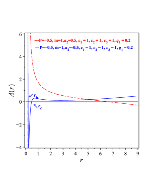
(a)  The function A(r) via the radial coordinate

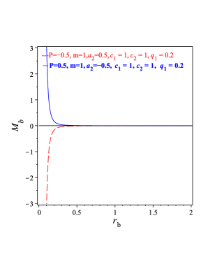
(b)  The horizon mass-radius relation

Figure 1: Schematic plot of horizons of solution (III.1). The plot of Fig.1 0(a) shows the black hole event horizon, $r_{b}$, and the cosmological horizon, $r_{c}$, while of Fig.1 0(b) shows the horizon-mass radius relation. Here we take $d=4$ and $a_{1}=1$.

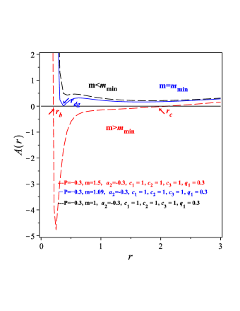
(a)  Possible horizons of the solution (III.1)

(b)  Horizon temperature–radius relation

Figure 2: Schematic plots of the degenerate horizons of solution (III.1): 1(a) The plot of $A(r)$ shows the black hole event horizon, $r_{b}$, and the cosmological horizon, $r_{c}$, where $m>m_{min}$. At $m=m_{min}$ ($r_{b}=r_{c}$), the black hole has a degenerate horizon at $r_{dg}$. Otherwise, $m<m_{min}$ the black hole is naked; 1(b) the temperature vanishes on the horizon radius $r_{b}$. Here we take $d=4$.

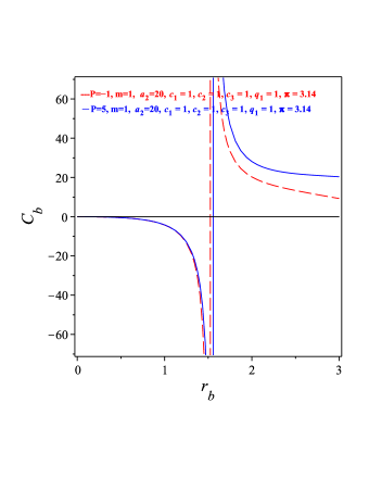
(a)  Horizon heat capacity–radius relation of black hole (III.1)

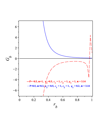
(b)  Gibbs free energy–radius relation of black hole (III.1)

Figure 3: Schematic plot of the heat capacity shows the locally unstable event horizon which is characterized by the negative $C_{h}<0$. Also, the plot shows a second-order phase transition as $C_{h}$ diverges; 2(b) shows free energy of black hole (III.1).

The Bekenstein-Hawking entropy for $f({\mathcal{T}})$ gravity can be defined as Miao et al. (2011)

$$S(r_{b})=\frac{1}{4}Af_{\mathcal{T}}=\pi r_{b}{}^{2}f_{\mathcal{T}},$$ (62)

where $r_{b}$ is the event horizon in Planck units and $A$ is the event horizon area. Using Eq. (III.1) in (62), we get

$$S(r_{b})\approx\frac{r_{b}{}^{d-2}\Omega_{d-2}}{6}\left[a_{1}-\frac{2\sqrt{3P|a_{2}|}}{r_{b}{}^{d-2}}+\frac{q_{1}{}^{2}\sqrt{3P|a_{2}|}}{(d-3)^{2}m^{2}r_{b}{}^{3d-8}}+O\Big{(}\frac{1}{r_{b}{}^{2(d-1)}}\Big{)}+\cdots\right],$$ (63)

where $\Omega_{d-2}$ is the volume of the unit $(d-2)$-sphere. Eq. (63) shows that, if we neglect the higher order terms of ${\mathcal{O}}\Big{(}\frac{1}{r_{b}{}^{2(d-1)}}\Big{)}$, the term $\left(a_{1}-\frac{2\sqrt{3P|a_{2}|}}{r_{b}{}^{d-2}}+\frac{q_{1}{}^{2}\sqrt{3P|a_{2}|}}{(d-3)^{2}m^{2}r_{b}{}^{3d-8}}\right)$ must be positive in order to have a positive entropy. This leads to $q_{1}\geq\frac{\pm mr_{h}{}^{d-3}\sqrt{x(2x-a_{1}r_{h}{}^{d-2})}}{x}$ and $x>\frac{a_{1}r_{b}{}^{d-2}}{2}$ where $x=\sqrt{3P|a_{2}|}$, otherwise we have a negative entropy.

The thermodynamical stability is related to the heat capacity $C_{b}$. In particular wth the sign of this quantity. Below, we will take into account the thermal stability of the black holes via their heat capacity Nouicer (2007); Dymnikova and Korpusik (2011); Chamblin et al. (1999)

$$C_{b}=\frac{dE_{b}}{dT_{b}}=\frac{\partial m}{\partial r_{b}}\left(\frac{\partial T}{\partial r_{b}}\right)^{-1},$$ (64)

where $E_{b}$ is the energy. If $C_{b}>0$ ($C_{b}<0$), the black hole is stable (unstable) from thermodynamical point of view. To better understand this phenomenon, let us assume that, due to thermal fluctuations, the black hole absorbs more radiation than it emits. When this happens, its heat capacity is positive. According to this situation, the black hole mass increases. On the other hand, if the black hole emits more radiation than it absorbs, the heat capacity becomes negative. In this situation, the black hole mass decreases and it can completely evaporate. In conclusion, black holes with negative heat capacities are unstable from a thermodynamical point of view.

In order to calculate Eq. (64), we have to derive the formulae of $M_{b}\equiv M(r_{b})$ and $T_{b}\equiv T(r_{b})$. Firstly, we calculate the black hole mass within an even horizon $r_{b}$. We set $A(r_{b})=0$, then we obtain

$${M_{b}}_{{}_{{}_{{}_{{}_{\tiny Eq.(\ref{df55})}}}}}=r_{b}{}^{d-3}\left(\Lambda_{eff}r_{b}{}^{2}+\frac{Q^{2}}{r_{b}{}^{2(d-3)}}+\frac{Q_{1}{}^{4}}{r_{b}{}^{(3d-8)}}+\frac{Q_{2}{}^{4}}{r_{b}{}^{4(d-3)}}+\cdots\right).$$ (65)

The above equation shows that the total mass of the black hole is given by a function of the charge and the horizon radius. It is straightforward to calculate the degenerate horizon by the condition $\partial M_{h}/\partial r_{b}=0$, which gives

$$r_{dg}=\pm\frac{(6a_{2}P)^{1/6}\sqrt{(3q_{1}{}^{2}a_{1}+4m^{2}\sqrt{3P|a_{2}|}+q_{1}\sqrt{a_{1}}\sqrt{9a_{1}q_{1}{}^{2}+24m^{2}\sqrt{3P|a_{2}|}})^{3/2}-2\sqrt{6}(m^{4}Pa_{2})^{1/3}}}{\sqrt{a_{1}}m^{1/3}(3a_{1}q_{1}{}^{2}+4m^{2}\sqrt{3P|a_{2}|}+q_{1}\sqrt{a1}\sqrt{9a_{1}q_{1}{}^{2}+24m^{2}\sqrt{3P|a_{2}|}})^{1/6}},$$

in $4$ dimensions. As seen from Eq. (65) and Fig.2 1(a), the horizon mass–radius relation is given by

$$M(r_{b}\rightarrow 0)\rightarrow\infty,\qquad\qquad M(r_{b}\rightarrow\infty)\rightarrow\infty.$$ (66)

The Hawking temperature of black holes is derived by requiring no singularity at the horizon of the Euclidean sector of solutions. Furthermore, it is possible to obtain the temperature related with the outer event horizon $r=r_{b}$ as Hawking (1975)

$$T=\frac{\kappa}{2\pi},\qquad\qquad\kappa=\frac{A^{\prime}(r_{b})}{2}.$$ (67)

where $\kappa$ is the surface gravity. The Hawking temperature associated with the black hole solution (III.1) is

$${T_{b}}_{{}_{{}_{{}_{{}_{\tiny Eq.(\ref{df55})}}}}} = \frac{1}{4\pi}\Bigg{\{}(d-1)r_{b}\Lambda_{eff}-\frac{(d-3)Q^{2}}{r_{b}^{2d-5}}-\frac{(2d-5)Q_{1}{}^{4}}{r_{b}{}^{(3d-7)}}+\frac{3(d-3)Q_{2}{}^{4}}{r_{b}{}^{(4d-11)}}+\cdots\Bigg{\}},$$

where ${T_{b}}$ is calculated at the event horizon. In Fig.2 1(b), it is shown that the horizon temperature $T_{h}$ is zero at the degenerate horizon $r_{b}=r_{dg}$. For $r_{b}<r_{dg}$, the horizon temperature evolves below the absolute zero giving rise to an ultra-cold black hole. As pointed out in Davies (1977), there is no reason from thermodynamical point of view to prevent a black hole temperature to go under absolute zero. In this case, the black hole would become a naked singularity. In the range $r_{b}>r_{dg}$, the horizon temperature is positive. Considering also gravitational effects, we obtain that, for some high temperature $T_{max}$, the radiation becomes unstable and the collapse starts Hawking and Page (1983). As a consequence, the AdS solution is stable only for $T<T_{max}$. Above $T_{max}$, only the heavy black holes reach stable configurations Hawking and Page (1983).

Let us now calculate the heat capacity $C_{b}h$ horizon and substitute Eqs. (65) and (V) into Eq. (64). We have

$${C_{b}}_{{}_{{}_{{}_{{}_{\tiny Eq.(\ref{df55})}}}}}\approx-4\pi r_{b}{}^{2}-\frac{288\pi(d-2)\alpha P}{r_{b}{}^{d-2}}+\frac{576\pi(d-2)\alpha P\sqrt{3P|\alpha|}}{r_{b}{}^{2(d-2)}}+\frac{288\pi(2d-5)\alpha q_{1}{}^{2}P}{(d-3)^{2}m^{2}r_{b}{}^{(3d-8)}}.$$ (69)

In Fig.3 2(a), it is shown that the heat capacity is negative for $r_{b}<r_{dg}$ and positive for $r_{b}>r_{dg}$. Always considering Fig.3 2(a), a characteristic of the heat capacity is a second-order phase transition at $r_{c}$ whereas the heat capacity shows an infinite discontinuity.

The Grand Canonical Ensemble free energy, that is the Gibbs free energy, is defined as Kim and Kim (2012)

$$G(r_{b})=M(r_{b})-T(r_{b})S(r_{b}),$$ (70)

where $M(r_{b})$, $T(r_{b})$ and $S(r_{b})$ are the mass, the temperature and the entropy of the black hole at the event horizon, respectively. Using Eqs. (62), (65) and (V) in Eq. (70), we get

$${G_{b}}_{{}_{{}_{{}_{{}_{\tiny Equation(\ref{df55})}}}}}=r_{b}{}^{d-3}\left(\Lambda_{eff}r_{b}{}^{2}+\frac{Q^{2}}{r_{b}{}^{2(d-3)}}+\frac{Q_{1}{}^{4}}{r_{b}{}^{(3d-8)}}+\frac{Q_{2}{}^{4}}{r_{b}{}^{4(d-3)}}+\cdots\right)+\Omega_{d-2}\Big{(}\frac{q^{2}r_{b}{}^{d-1}(d-3)^{2}}{144(c-2)c_{1}\alpha}-\frac{q^{2}r_{b}(d-3)^{2}\sqrt{3P|\alpha|}}{72(d-2)c_{1}\alpha}$$

$$+\frac{P}{36(d-2)^{3}c_{1}r_{b}^{d-3}}+\frac{q^{2}\sqrt{3P|\alpha|}}{144m^{2}(d-2)r_{b}^{2d-7}c_{1}\alpha}-\frac{5(d-3)^{2}Pq^{2}\sqrt{3P|\alpha|}}{6(d-2)r_{b}^{2b-5}c_{1}\alpha}\Big{)}.$$ (71)

It is worth noticing that, as soon as the charge parameter $q_{1}\rightarrow 0$, the Gibbs free energy derived from Eqs. (III.1) is coincident with that in Altamirano et al. (2014). The Gibbs energy of our solution is represented in Fig.3 2(b) for some values of model parameters.

VI Discussion and conclusions

In this paper, we have investigated the effect of the non-linear electrodynamics on modified TEGR theory. To this aim, we derived the charged non-linear electrodynamics field equations for $f({\mathcal{T}})$ gravity. They reduce to the well known form of Maxwell field equations assuming some constrains on the arbitrary functions. Applying these field equations to cylindrical coordinates in $d$–dimensions, we got a closed system of non-linear differential equations. In this framework, we obtained black hole solutions. The most interesting feature of thes black hole solutions is that they behave as AdS solutions generalizing the black hole solutions derived in Awad et al. (2017). This generalization comes from the contribution of the parameter included in the arbitrary function (30). If this parameter set equal to zero we return to the black black hole presented in Awad et al. (2017). The contributions of non-linear electrodynamics clearly emerge in the above black holes discriminating the solutions with respect to the standard Maxwell field. Our black holes keep all the features of the black holes derived in Awad et al. (2017), i.e., they shows a central singularity, that is softer in comparison with the standard GR and TEGR cases. The rotating black hole solutions can be achieved by a suitable coordinate transformation.

More information on the black hole (III.1) is obtained by its thermodynamical properties. The most important feature in $f({\mathcal{T}})$ gravity is that entropy is not always proportional to the horizon area Cvetič et al. (2002); Nojiri et al. (2001). It is possible to show that, for constraints on the parameter $q_{1}$ characterizing the arbitrary function of the non-linear electrodynamics, one has a positive entropy. On the other hand, there are some regions of parameter $q_{1}$ where entropy is negative Cvetič et al. (2002); Nojiri and Odintsov (2002, 2017); Clunan et al. (2004). Negative entropy is a familiar feature in gravitational theories: several black hole solutions have negative entropy, e.g. charged Gauss-Bonnet AdS black holes Cvetič et al. (2002); Nojiri et al. (2002); Nojiri and Odintsov (2002, 2017). Our results indicate that negative entropies may be explained as a region where the parameter $q_{1}$ values have entered into an un-allowed region, or into a regime where there is a phase transition. The gravitational entropy of non-trivial solutions in $f({\mathcal{T}})$ gravity will be the subject of future researches.

Furthermore, the heat capacity of black hole (III.1) has been derived and we have shown that there is a locally unstable event horizon characterized by $C_{b}<0$. Furthermore there is a second-order phase transition at $r_{b}$ whereas the heat capacity is characterized by an infinite discontinuity. Finally, the heat capacity of our black hole has a stable event horizon which is characterized by a positive value, i.e., $C_{b}>0$ for which $r_{b}>r_{dg}$. Finally, we have derived the Gibbs free energy showing that the black hole solution (III.1) has always a positive value of this quantity for some constrains on the parameter as Fig.3 2(b) shows. In a forthcoming study, possible astrophysical applications of these solutions will be considered.

References

- Awad et al. (2017) A. M. Awad, S. Capozziello, and G. G. L. Nashed, “D-dimensional charged Anti-de-Sitter black holes in gravity,” Journal of High Energy Physics 7, 136 (2017), arXiv:1706.01773 [gr-qc] .
- Farrugia et al. (2016) G. Farrugia, J. L. Said, and M. L. Ruggiero, “Solar System tests in gravity,” Phys. Rev. D 93, 104034 (2016), arXiv:1605.07614 [gr-qc] .
- Riess et al. (1998) A. G. Riess et al. (Supernova Search Team), “Observational evidence from supernovae for an accelerating universe and a cosmological constant,” Astron. J. 116, 1009–1038 (1998), arXiv:astro-ph/9805201 [astro-ph] .
- Perlmutter et al. (1999) S. Perlmutter, G. Aldering, G. Goldhaber, R. A. Knop, P. Nugent, P. G. Castro, S. Deustua, S. Fabbro, A. Goobar, D. E. Groom, I. M. Hook, A. G. Kim, M. Y. Kim, J. C. Lee, N. J. Nunes, R. Pain, C. R. Pennypacker, R. Quimby, C. Lidman, R. S. Ellis, M. Irwin, R. G. McMahon, P. Ruiz-Lapuente, N. Walton, B. Schaefer, B. J. Boyle, A. V. Filippenko, T. Matheson, A. S. Fruchter, N. Panagia, H. J. M. Newberg, W. J. Couch, and T. S. C. Project, “Measurements of and from 42 High-Redshift Supernovae,” Astrophys. J. 517, 565–586 (1999), astro-ph/9812133 .
- Hinshaw et al. (2013) G. Hinshaw, D. Larson, E. Komatsu, D. N. Spergel, C. L. Bennett, J. Dunkley, M. R. Nolta, M. Halpern, R. S. Hill, N. Odegard, L. Page, K. M. Smith, J. L. Weiland, B. Gold, N. Jarosik, A. Kogut, M. Limon, S. S. Meyer, G. S. Tucker, E. Wollack, and E. L. Wright, “Nine-year Wilkinson Microwave Anisotropy Probe (WMAP) Observations: Cosmological Parameter Results,” apjs 208, 19 (2013), arXiv:1212.5226 .
- Eisenstein et al. (2005) D. J. Eisenstein et al. (SDSS), “Detection of the Baryon Acoustic Peak in the Large-Scale Correlation Function of SDSS Luminous Red Galaxies,” Astrophys. J. 633, 560–574 (2005), arXiv:astro-ph/0501171 [astro-ph] .
- Wang (2008) Y. Wang, “Model-independent distance measurements from gamma-ray bursts and constraints on dark energy,” Phys. Rev. D 78, 123532 (2008), arXiv:0809.0657 .
- Peebles and Ratra (2003) P. J. Peebles and B. Ratra, “The cosmological constant and dark energy,” Reviews of Modern Physics 75, 559–606 (2003), astro-ph/0207347 .
- Binney and Tremaine (1987) J. Binney and S. Tremaine, Princeton, NJ, Princeton University Press, 1987, 747 p. (1987).
- Will (2014) C. M. Will, “Was Einstein Right? A Centenary Assessment,” arXiv e-prints (2014), arXiv:1409.7871 [gr-qc] .
- Capozziello and Francaviglia (2008) S. Capozziello and M. Francaviglia, “Extended theories of gravity and their cosmological and astrophysical applications,” General Relativity and Gravitation 40, 357–420 (2008), arXiv:0706.1146 .
- de Andrade et al. (2000) V. C. de Andrade, L. C. T. Guillen, and J. G. Pereira, “Teleparallel Gravity: An Overview,” arXiv General Relativity and Quantum Cosmology e-prints (2000), gr-qc/0011087 .
- Nashed (2018) Gamal Nashed, “Charged and Non-Charged Black Hole Solutions in Mimetic Gravitational Theory,” Symmetry 10, 559 (2018).
- Aldrovandi et al. (2003) R. Aldrovandi, J. G. Pereira, and K. H. Vu, “Selected Topics in Teleparallel Gravity,” arXiv General Relativity and Quantum Cosmology e-prints (2003), gr-qc/0312008 .
- Maluf (2013) J. W. Maluf, “The teleparallel equivalent of general relativity,” Annalen der Physik 525, 339–357 (2013), arXiv:1303.3897 [gr-qc] .
- Unzicker and Case (2005) A. Unzicker and T. Case, “Translation of Einstein’s Attempt of a Unified Field Theory with Teleparallelism,” ArXiv Physics e-prints (2005), physics/0503046 .
- Nashed (2003) Gamal G. L. Nashed, “Stability of the vacuum nonsingular black hole,” Chaos Solitons Fractals 15, 841 (2003), arXiv:gr-qc/0301008 [gr-qc] .
- de Andrade and Pereira (1997) V. C. de Andrade and J. G. Pereira, “Gravitational Lorentz force and the description of the gravitational interaction,” Phys. Rev. D 56, 4689–4695 (1997), gr-qc/9703059 .
- Mai and Lü (2017) Z.-F. Mai and H. Lü, “Black holes, dark wormholes, and solitons in gravities,” Phys. Rev. D 95, 124024 (2017), arXiv:1704.05919 [hep-th] .
- Ferraro and Fiorini (2008) R. Ferraro and F. Fiorini, “Born-Infeld gravity in Weitzenböck spacetime,” Phys. Rev. D 78, 124019 (2008), arXiv:0812.1981 [gr-qc] .
- Fiorini and Ferraro (2009) F. Fiorini and R. Ferraro, “a Type of Born-Infeld Regular Gravity and its Cosmological Consequences,” International Journal of Modern Physics A 24, 1686–1689 (2009), arXiv:0904.1767 [gr-qc] .
- Cardone et al. (2012) V. F. Cardone, N. Radicella, and S. Camera, “Accelerating f(T) gravity models constrained by recent cosmological data,” Phys. Rev. D 85, 124007 (2012), arXiv:1204.5294 .
- Myrzakulov (2011) R. Myrzakulov, “Accelerating universe from gravity,” European Physical Journal C 71, 1752 (2011), arXiv:1006.1120 [gr-qc] .
- Nashed and El Hanafy (2017) G. G. L. Nashed and W. El Hanafy, “Analytic rotating black hole solutions in -dimensional gravity,” Eur. Phys. J. C77, 90 (2017), arXiv:1612.05106 [gr-qc] .
- Yang (2011) R.-J. Yang, “New types of f( T) gravity,” European Physical Journal C 71, 1797 (2011), arXiv:1007.3571 [gr-qc] .
- Bengochea (2011) G. R. Bengochea, “Observational information for theories and dark torsion,” Physics Letters B 695, 405–411 (2011), arXiv:1008.3188 [astro-ph.CO] .
- Bamba et al. (2010) K. Bamba, C.-Q. Geng, and C.-C. Lee, “Generic feature of future crossing of phantom divide in viable gravity models,” jcap 11, 001 (2010), arXiv:1007.0482 .
- Karami and Abdolmaleki (2013) K. Karami and A. Abdolmaleki, “ modified teleparallel gravity as an alternative for holographic and new agegraphic dark energy models,” Research in Astronomy and Astrophysics 13, 757-771 (2013), arXiv:1009.2459 [gr-qc] .
- Dent et al. (2011) J. B. Dent, S. Dutta, and E. N. Saridakis, “ gravity mimicking dynamical dark energy. Background and perturbation analysis,” jcap 1, 009 (2011), arXiv:1010.2215 [astro-ph.CO] .
- Cai et al. (2011) Y.-F. Cai, S.-H. Chen, J. B. Dent, S. Dutta, and E. N. Saridakis, “Matter bounce cosmology with the gravity,” Classical and Quantum Gravity 28, 215011 (2011), arXiv:1104.4349 [astro-ph.CO] .
- Capozziello et al. (2011) S. Capozziello, V. F. Cardone, H. Farajollahi, and A. Ravanpak, “Cosmography in gravity,” Phys. Rev. D 84, 043527 (2011), arXiv:1108.2789 [astro-ph.CO] .
- Bamba et al. (2013) K. Bamba, S. D. Odintsov, and D. Sáez-Gómez, “Conformal symmetry and accelerating cosmology in teleparallel gravity,” Phys. Rev. D 88, 084042 (2013), arXiv:1308.5789 [gr-qc] .
- Camera et al. (2014) S. Camera, V. F. Cardone, and N. Radicella, “Detectability of torsion gravity via galaxy clustering and cosmic shear measurements,” Phys. Rev. D 89, 083520 (2014), arXiv:1311.1004 .
- Nashed (2015) G. L. Nashed, “FRW in quadratic form of gravitational theories,” Gen. Rel. Grav. 47, 75 (2015), arXiv:1506.08695 [gr-qc] .
- Nashed (2013a) G. G. L. Nashed, “Spherically symmetric charged-dS solution in gravity theories,” Phys. Rev. D 88, 104034 (2013a), arXiv:1311.3131 [gr-qc] .
- Shirafuji et al. (1996) T. Shirafuji, G. G. Nashed, and K. Hayashi, “Energy of General Spherically Symmetric Solution in the Tetrad Theory of Gravitation,” Progress of Theoretical Physics 95, 665–678 (1996), gr-qc/9601044 .
- Wang (2011) T. Wang, “Static solutions with spherical symmetry in theories,” Phys. Rev. D 84, 024042 (2011), arXiv:1102.4410 [gr-qc] .
- Ferraro and Fiorini (2011) R. Ferraro and F. Fiorini, “Spherically symmetric static spacetimes in vacuum gravity,” Phys. Rev. D 84, 083518 (2011), arXiv:1109.4209 [gr-qc] .
- Nashed et al. (2019) G. G. L. Nashed, W. El Hanafy, and Kazuharu Bamba, “Charged rotating black holes coupled with nonlinear electrodynamics Maxwell field in the mimetic gravity,” JCAP 1901, 058 (2019), arXiv:1809.02289 [gr-qc] .
- Iorio et al. (2015) L. Iorio, N. Radicella, and M. L. Ruggiero, “Constraining gravity in the solar system,” Journal of Cosmology and Astroparticle Physics 2015, 021–021 (2015).
- Nashed and Capozziello (2018) G. G. L. Nashed and S. Capozziello, “Charged Anti-de Sitter BTZ black holes in Maxwell- gravity,” Int. J. Mod. Phys. A33, 1850076 (2018), arXiv:1710.06620 [gr-qc] .
- Awad et al. (2018) A. Awad, W. El Hanafy, G.G.L. Nashed, and Emmanuel N. Saridakis, “Phase portraits of general cosmology,” Journal of Cosmology and Astroparticle Physics 2018, 052–052 (2018).
- González et al. (2012) P. A. González, E. N. Saridakis, and Y. Vásquez, “Circularly symmetric solutions in three-dimensional teleparallel, and Maxwell- gravity,” Journal of High Energy Physics 7, 53 (2012), arXiv:1110.4024 [gr-qc] .
- Awad et al. (2019) A. M. Awad, G. G. L. Nashed, and W. El Hanafy, “Rotating charged ads solutions in quadratic gravity,” The European Physical Journal C 79, 668 (2019).
- Hanafy and Nashed (2017) W. El Hanafy and G.G.L. Nashed, “Generic phase portrait analysis of finite-time singularities and generalized teleparallel gravity,” Chinese Physics C 41, 125103 (2017).
- Iorio et al. (2016) L. Iorio, M. L. Ruggiero, N. Radicella, and E. N. Saridakis, “Constraining the Schwarzschild de Sitter solution in models of modified gravity,” Physics of the Dark Universe 13, 111 – 120 (2016).
- Junior et al. (2015) E. L. B. Junior, M. E. Rodrigues, and M. J.S. Houndjo, “Born-infeld and charged black holes with non-linear source in gravity,” Journal of Cosmology and Astroparticle Physics 2015, 037–037 (2015).
- Harko et al. (2014) T. Harko, F. S. N. Lobo, G. Otalora, and E. N. Saridakis, “ gravity and cosmology,” Journal of Cosmology and Astroparticle Physics 2014, 021–021 (2014).
- Capozziello et al. (2013) S. Capozziello, P. A. Gonzalez, E.l N. Saridakis, and Y. Vasquez, “Exact charged black-hole solutions in D-dimensional gravity: torsion vs curvature analysis,” JHEP 02, 039 (2013), arXiv:1210.1098 [hep-th] .
- Rodrigues et al. (2013) M. E. Rodrigues, M. J. S. Houndjo, J. Tossa, D. Momeni, and R. Myrzakulov, “Charged black holes in generalized teleparallel gravity,” jcap 11, 024 (2013), arXiv:1306.2280 [gr-qc] .
- Nashed (2013b) G. G. L. Nashed, “A special exact spherically symmetric solution in gravity theories,” General Relativity and Gravitation 45, 1887–1899 (2013b), arXiv:1502.05219 [gr-qc] .
- Nashed (2010) G. G. L. Nashed, “Stationary axisymmetric solutions and their energy contents in teleparallel equivalent of Einstein theory,” apss 330, 173–181 (2010), arXiv:1503.01379 [gr-qc] .
- Junior et al. (2015) E. L. B. Junior, M. E. Rodrigues, and M. J. S. Houndjo, “Regular black holes in gravity through a nonlinear electrodynamics source,” jcap 10, 060 (2015), arXiv:1503.07857 [gr-qc] .
- Bejarano et al. (2015) C. Bejarano, R. Ferraro, and M. J. Guzmán, “Kerr geometry in gravity,” European Physical Journal C 75, 77 (2015), arXiv:1412.0641 [gr-qc] .
- Gamal (2012) G. L. N. Gamal, “Spherically Symmetric Solutions on a Non-Trivial Frame in Theories of Gravity,” Chinese Physics Letters 29, 050402 (2012), arXiv:1111.0003 [physics.gen-ph] .
- Nashed (2014) G. G. L. Nashed, “Schwarzschild solution in extended teleparallel gravity,” EPL (Europhysics Letters) 105, 10001 (2014), arXiv:1501.00974 [gr-qc] .
- Iorio and Saridakis (2012) L. Iorio and E. N. Saridakis, “Solar system constraints on gravity,” mnras 427, 1555–1561 (2012), arXiv:1203.5781 [gr-qc] .
- Xie and Deng (2013) Y. Xie and X.-M. Deng, “ gravity: effects on astronomical observations and Solar system experiments and upper bounds,” mnras 433, 3584–3589 (2013), arXiv:1312.4103 [gr-qc] .
- Tamanini and Böhmer (2012) N. Tamanini and C. G. Böhmer, “Good and bad tetrads in gravity,” Phys. Rev. D 86, 044009 (2012), arXiv:1204.4593 [gr-qc] .
- Ruggiero and Radicella (2015) M. L. Ruggiero and N. Radicella, “Weak-field spherically symmetric solutions in gravity,” Phys. Rev. D 91, 104014 (2015), arXiv:1501.02198 [gr-qc] .
- Iorio et al. (2015) L. Iorio, N. Radicella, and M. L. Ruggiero, “Constraining gravity in the Solar System,” jcap 8, 021 (2015), arXiv:1505.06996 [gr-qc] .
- Nashed and Saridakis (2019) G. G. L. Nashed and E. N. Saridakis, “Rotating AdS black holes in Maxwell- gravity,” Class. Quant. Grav. 36, 135005 (2019), arXiv:1811.03658 [gr-qc] .
- Plebański (1970) J. Plebański, Lectures on non-linear electrodynamics: an extended version of lectures given at the Niels Bohr Institute and NORDITA, Copenhagen, in October 1968 (NORDITA, 1970).
- Ayon-Beato (1999) E. Ayon-Beato, “New regular black hole solution from nonlinear electrodynamics,” Physics Letters B 464, 25–29 (1999), hep-th/9911174 .
- Salazar I. et al. (1987) H. Salazar I., A. García D., and J. Plebański, “Duality rotations and type D solutions to Einstein equations with nonlinear electromagnetic sources,” Journal of Mathematical Physics 28, 2171–2181 (1987).
- Nesseris et al. (2013) S. Nesseris, S. Basilakos, E. N. Saridakis, and L. Perivolaropoulos, “Viable models are practically indistinguishable from CDM,” Phys. Rev. D 88, 103010 (2013), arXiv:1308.6142 [astro-ph.CO] .
- Nunes et al. (2016) R. C. Nunes, S. Pan, and E. N. Saridakis, “New observational constraints on gravity from cosmic chronometers,” jcap 8, 011 (2016), arXiv:1606.04359 [gr-qc] .
- Basilakos et al. (2018) S. Basilakos, S. Nesseris, F. K. Anagnostopoulos, and E. N. Saridakis, “Updated constraints on models using direct and indirect measurements of the Hubble parameter,” jcap 8, 008 (2018), arXiv:1803.09278 .
- Lemos (1995) J. P. S. Lemos, “Cylindrical black hole in general relativity,” Phys. Lett. , 46–51 (1995), arXiv:gr-qc/9404041 [gr-qc] .
- Awad (2003) Adel M. Awad, “Higher dimensional charged rotating solutions in (A)dS space-times,” Class. Quant. Grav. 20, 2827–2834 (2003), arXiv:hep-th/0209238 [hep-th] .
- Hunter (1999) C. J. Hunter, “The Action of instantons with nut charge,” Phys. Rev. , 024009 (1999), arXiv:gr-qc/9807010 [gr-qc] .
- Hawking et al. (1999) S. W. Hawking, C. J. Hunter, and Don N. Page, “Nut charge, anti-de Sitter space and entropy,” Phys. Rev. , 044033 (1999), arXiv:hep-th/9809035 [hep-th] .
- Bekenstein (1972) J. D. Bekenstein, “Black holes and the second law,” Lett. Nuovo Cim. 4, 737–740 (1972).
- Bekenstein (1973) Jacob D. Bekenstein, “Black holes and entropy,” Phys. Rev. , 2333–2346 (1973).
- Gibbons and Hawking (1977) G. W. Gibbons and S. W. Hawking, “Cosmological Event Horizons, Thermodynamics, and Particle Creation,” Phys. Rev. , 2738–2751 (1977).
- Dymnikova (1996) I. Dymnikova, “De Sitter-Schwarzschild Black Hole:. its Particlelike Core and Thermodynamical Properties,” International Journal of Modern Physics D 5, 529–540 (1996).
- Dymnikova (2002) I. Dymnikova, “Cosmological term as a source of mass,” Class. Quant. Grav. 19, 725–740 (2002), arXiv:gr-qc/0112052 [gr-qc] .
- Dymnikova (2018) I. Dymnikova, “Generic Features of Thermodynamics of Horizons in Regular Spherical Space-Times of the Kerr-Schild Class,” Universe 4, 63 (2018).
- Ghaderi and Malakolkalami (2016) K. Ghaderi and B. Malakolkalami, “Thermodynamics of the Schwarzschild and the Reissnerï¿œNordstrï¿œm black holes with quintessence,” Nucl. Phys. , 10–18 (2016).
- Hayward (2006) S. A. Hayward, “Formation and evaporation of regular black holes,” Phys. Rev. Lett. 96, 031103 (2006), arXiv:gr-qc/0506126 [gr-qc] .
- Kim et al. (2008) W. Kim, H. Shin, and M. Yoon, “Anomaly and Hawking radiation from regular black holes,” J. Korean Phys. Soc. 53, 1791–1796 (2008), arXiv:0803.3849 [gr-qc] .
- Myung et al. (2009) Y. Soo Myung, Y.-Wan Kim, and Y.-Jai Park, “Thermodynamics of regular black hole,” Gen. Rel. Grav. 41, 1051–1067 (2009), arXiv:0708.3145 [gr-qc] .
- Nicolini et al. (2006) P. Nicolini, A. Smailagic, and E. Spallucci, “Noncommutative geometry inspired Schwarzschild black hole,” Phys. Lett. , 547–551 (2006), arXiv:gr-qc/0510112 [gr-qc] .
- Sharif and Javed (2011) M. Sharif and Wajiha Javed, “Thermodynamics of a Bardeen black hole in noncommutative space,” Can. J. Phys. 89, 1027–1033 (2011), arXiv:1109.6627 [gr-qc] .
- Miao et al. (2011) R.-X. Miao, M. Li, and Y.-G. Miao, “Violation of the first law of black hole thermodynamics in gravity,” jcap 11, 033 (2011), arXiv:1107.0515 [hep-th] .
- Nouicer (2007) K. Nouicer, “Black holes thermodynamics to all order in the Planck length in extra dimensions,” Class. Quant. Grav. 24, 5917–5934 (2007), [Erratum: Class. Quant. Grav.24,6435(2007)], arXiv:0706.2749 [gr-qc] .
- Dymnikova and Korpusik (2011) I. Dymnikova and M. Korpusik, “Thermodynamics of regular cosmological black holes with the de sitter interior,” Entropy 13, 1967–1991 (2011).
- Chamblin et al. (1999) A. Chamblin, R. Emparan, C. V. Johnson, and R. C. Myers, “Charged AdS black holes and catastrophic holography,” Phys. Rev. , 064018 (1999), arXiv:hep-th/9902170 [hep-th] .
- Hawking (1975) S. W. Hawking, “Particle Creation by Black Holes,” Euclidean quantum gravity, Commun. Math. Phys. 43, 199–220 (1975), [,167(1975)].
- Davies (1977) P. C. W. Davies, “Thermodynamics of Black Holes,” Proc. Roy. Soc. Lond. , 499–521 (1977).
- Hawking and Page (1983) S. W. Hawking and Don N. Page, “Thermodynamics of Black Holes in anti-De Sitter Space,” Commun. Math. Phys. 87, 577 (1983).
- Kim and Kim (2012) W. Kim and Y. Kim, “Phase transition of quantum-corrected Schwarzschild black hole,” Physics Letters B 718, 687–691 (2012), arXiv:1207.5318 [gr-qc] .
- Altamirano et al. (2014) N. Altamirano, D. Kubizňák, R. Mann, and Z. Sherkatghanad, “Thermodynamics of Rotating Black Holes and Black Rings: Phase Transitions and Thermodynamic Volume,” Galaxies 2, 89–159 (2014), arXiv:1401.2586 [hep-th] .
- Cvetič et al. (2002) M. Cvetič, S. Nojiri, and S. D. Odintsov, “Black hole thermodynamics and negative entropy in de sitter and anti-de sitter einstein-gauss-bonnet gravity,” Nuclear Physics B 628, 295–330 (2002), hep-th/0112045 .
- Nojiri et al. (2001) S. Nojiri, S. D. Odintsov, and S. Ogushi, “Holographic Entropy and Brane FRW Dynamics from AdS Black Hole in d5 Higher Derivative Gravity,” International Journal of Modern Physics A 16, 5085–5099 (2001), hep-th/0105117 .
- Nojiri and Odintsov (2002) S. Nojiri and S. D. Odintsov, “(Anti-)de Sitter black holes in higher derivative gravity and dual conformal field theories,” Phys. Rev. D 66, 044012 (2002), hep-th/0204112 .
- Nojiri and Odintsov (2017) S. Nojiri and S. D. Odintsov, “Regular multihorizon black holes in modified gravity with nonlinear electrodynamics,” Phys. Rev. D 96, 104008 (2017), arXiv:1708.05226 [hep-th] .
- Clunan et al. (2004) T. Clunan, S. F. Ross, and D. J. Smith, “On Gauss Bonnet black hole entropy,” Classical and Quantum Gravity 21, 3447–3458 (2004), gr-qc/0402044 .
- Nojiri et al. (2002) S. Nojiri, S. D. Odintsov, and S. Ogushi, “Graviton correlator and metric perturbations in a de Sitter brane-world,” Phys. Rev. D 66, 023522 (2002), hep-th/0202098 .