PAC-Bayes with Backprop

Abstract

We explore the family of methods ‘PAC-Bayes with Backprop’ (PBB) to train probabilistic neural networks by minimizing PAC-Bayes bounds. We present two training objectives, one derived from a previously known PAC-Bayes bound, and a second one derived from a novel PAC-Bayes bound. Both training objectives are evaluated on MNIST and on various UCI data sets. Our experiments show two striking observations: we obtain competitive test set error estimates ($\sim 1.4\%$ on MNIST) and at the same time we compute non-vacuous bounds with much tighter values ($\sim 2.3\%$ on MNIST) than previous results. These observations suggest that neural nets trained by PBB may lead to self-bounding learning, where the available data can be used to simultaneously learn a predictor and certify its risk, with no need to follow a data-splitting protocol.

1 Introduction

In a probabilistic neural network the weights are random outcomes of a probability distribution, rather than having fixed deterministic values. For instance this may be realized by injecting noise into the components of a fixed architecture. The justification is that a probabilistic neural network may lead to better predictions, overcoming the limited generalization ability of a single weight vector (Neal [1993]). Other arguments in favour of weight randomization might be enforcing or studying robustness properties (Noy and Crammer [2014], Blundell et al. [2015], Zhang et al. [2019]), and making available better tools for the design and analysis of learning algorithms.

In this paper we take on probabilistic neural networks from a PAC-Bayes point of view. We focus on the family of methods ‘PAC-Bayes with Backprop’ (PBB) which derives training objectives based on PAC-Bayes upper bounds on the risk. The notable contributions of Dziugaite and Roy [2017, 2018] showed that exploring this approach is totally worth the while. Computational considerations aside, a clear advantage of PBB methods is being an instance of learning with guarantees: When training neural nets by PBB methods the output of the optimization process is a (randomized) predictor and simultaneously a risk certificate that guarantees its performance on unseen examples. Naturally, learning with guarantees per se will not impress until the values of the reported risk certificates match or closely follow the error estimates calculated on a test set, so that the former can be considered to be informative of the performance on unseen examples.

The results presented in this paper indicate a positive step towards learning with guarantees. We report experimental results on MNIST with two training objectives. The first training objective follows the PAC-Bayes-$\lambda$ bound of Thiemann et al. [2017]. The second training objective comes from what we call the PAC-Bayes-quadratic bound, whose derivation involves solving a quadratic inequality, hence the name. Our conclusions from these experiments are (1) that PBB methods achieve competitive (e.g. comparable to Blundell et al. [2015]’s) test set error estimates ($\sim 0.014$ on MNIST), while (2) the minimal value of the upper bound that we achieve ($\sim 0.023$ on MNIST) is a significant improvement over previous (e.g. Dziugaite and Roy [2017, 2018]’s) results, i.e. we further close the gap between the risk bound certificate and the test set risk estimate.

Our contributions:

1. Proposing two new training objectives for NNs: one derived from the PAC-Bayes-lambda bound, and one derived from the novel PAC-Bayes-quadratic bound.

2. Connecting Blundell et al. [2015]’s training method, which achieved competitive test set performance, to PAC-Bayes methods, which additionally produce a risk certificate and overcome some limitations of the former method, while also achieving competitive test set error estimates.

3. Demonstrating via experimental results that the family of methods ”PAC-Bayes with Backprop” might be able to achieve self-bounding learning: obtaining competitive test set error estimates and simultaneously computing non-vacuous bounds with much tighter values than previous works.

We would also like to highlight the elegant simplicity of the training methods we present here: our results are achieved with the classical fixed ‘data-free’ priors and classical SGD optimization (in contrast, Dziugaite and Roy [2018] used a special kind of data-dependent priors, and optimization via SGLD). Besides, our methods do not involve tampering with the training objective (in contrast, Blundell et al. [2015] used a “KL killing trick” by inserting a tunable parameter in their objective). This does not imply that extra resources do not have a valuable effect, but rather makes the point that it is indeed worthwhile studying simple methods, not just to understand their scope but also to more accurately assess the real value added by the extra resources.

Another set of experiments was run on five UCI datasets with the same two training objectives as our experiments on MNIST, again showing tightness of the gap between risk certificate and test set risk estimate. However, some initial experiments (not reported here) on CIFAR-10 gave risk certificates of three times the corresponding test set error estimate, which indicates that more needs to be done before ‘self-bounding learning’ can really be claimed.

The rest of this paper is organized as follows. In Section 2 we briefly recall some notions of the supervised learning framework, mainly to set the notation used later. Then in Section 3 we discuss the PAC-Bayes framework and two PAC-Bayes bounds. Section 4 presents two training objectives derived from the PAC-Bayes bounds. Section 5 discusses Blundell et al. [2015]’s objective. In Section 6 we presents our experimental results for both methods. We conclude and discuss future research directions in Section 7. Appendix A displays two KL divergence formulas for convenience. Appendix B presents the results of another set of experiments on some UCI data sets.

2 Generalization through risk upper bounds

In the context of supervised learning, an algorithm that trains a neural network receives a finite list of training examples and produces a weight vector $w\in\mathcal{W}\subset\mathbb{R}^{p}$ which will be used to predict the label of unseen examples. The ultimate goal is for the algorithm to find a weight that generalizes well, meaning that the decisions arrived at by using the learned $w$ should give rise to a small loss on unseen examples. Turning this into precise statements requires some formalizations, briefly discussed next. The experienced readers should feel free to skip the next couple of paragraphs which aim to recall these formalizations as well as setting the notation for the rest of the paper.

The training algorithm receives a size-$n$ list of labelled examples $Z_{1:n}=(Z_{1},\ldots,Z_{n})$, where the examples $Z_{i}$ are randomly drawn from a space $\mathcal{Z}$ according to an unknown underlying probability distribution $P\in M_{1}(\mathcal{Z})$. The form of the example space in supervised learning is $\mathcal{Z}=\mathcal{X}\times\mathcal{Y}$ with $\mathcal{X}\subset\mathbb{R}^{d}$ and $\mathcal{Y}\subset\mathbb{R}$, each example being a pair $Z_{i}=(X_{i},Y_{i})$ consisting of an input $X_{i}$ and its corresponding label $Y_{i}$. A space $\mathcal{W}$ encompasses all possible weight vectors, and it is understood that each possible weight vector $w\in\mathcal{W}$ maps to a function $h_{w}:\mathcal{X}\to\mathcal{Y}$ that will assign a label $h_{w}(X)\in\mathcal{Y}$ to each new input $X\in\mathcal{X}$. While statistical inference is largely concerned with learning properties of the unknown data-generating distribution, the main focus of machine learning is on the quality of predictors, measured by the expected loss on unseen examples, also called the risk:

$$L(w)=\operatorname{\mathbb{E}}[\ell(w,Z)]=\int_{\mathcal{Z}}\ell(w,z)P(dz)\,.$$ (1)

Here $\ell:\mathcal{W}\times\mathcal{Z}\to[0,\infty)$ is a fixed loss function. With these components, regression is defined as the problem when $\mathcal{Y}=\mathbb{R}$ and the loss function is the squared loss $\ell(w,z)=(y-h_{w}(x))^{2}$, while binary classification is defined with $\mathcal{Y}=\{0,1\}$ (or $\mathcal{Y}=\{-1,+1\}$) and setting the loss to the zero-one loss: $\ell(w,z)=\mathbb{I}[y\neq h_{w}(x)]$.

The goal of learning is to find a weight vector with small risk $L(w)$. Since the data-generating distribution $P$ is unknown, $L(w)$ is an unobservable objective. Replacing the expected loss with the average loss on the data gives rise to an observable objective called the empirical risk functional:

$$\hat{L}_{n}(w)=\hat{L}(w,Z_{1:n})=\frac{1}{n}\sum_{i=1}^{n}\ell(w,Z_{i})\,.$$ (2)

In practice, the minimization of $\hat{L}$ is often done with some version of gradient descent. Since the zero-one loss gives rise to a piecewise constant loss function, in classification it is common to replace it with a smooth(er) loss, such as the cross-entropy loss, while changing the range of $h_{w}$ to $[0,1]$.

Under certain conditions, minimizing the empirical risk leads to a weight that is guaranteed to have a small risk. Examples of such conditions are when the set of functions $\{h_{w}\,:\,w\in\mathbb{R}^{p}\}$ representable has a small capacity relative to the sample size or the map that produces the weights given the data is stable, or the same map is implicitly constructed by an algorithm such as stochastic gradient descent (see e.g. Bottou [2012] and references). However, oftentimes minimizing the empirical risk can lead to a situation when the risk of the learned weight is larger than desired – a case of overfitting. To prevent overfitting, various methods are commonly used. These include complexity regularization, early stopping, injecting noise in various places into the learning process, etc (e.g. Srivastava et al. [2014], Wan et al. [2013], Caruana et al. [2001], Hinton and van Camp [1993]).

An alternative to these is to minimize a surrogate objective which is guaranteed to give an upper bound on the risk. As long as the upper bound is tight and the optimization gives rise to a small value for the surrogate objective, the user can be sure that the risk will also be small: In this sense, overfitting is automatically prevented, while we also automatically get a self-bounded method in the sense of Freund [1998] (see also Langford and Blum [2003]). In this paper we follow this last approach, with two specific training objectives derived from corresponding PAC-Bayes bounds, which we introduce in the next section.

3 Two PAC-Bayes bounds

Probabilistic neural networks are realized as probability distributions over the weight space. While a classical neural network learns a data-dependent weight vector $\hat{w}$, a probabilistic neural network learns a data-dependent distribution over weights, say $Q\in M_{1}(\mathcal{W})$, and makes randomized predictions according to this distribution. To make a prediction on a fresh example $X$ the randomized predictor draws a weight vector $W$ at random according to $Q$ and applies $h_{W}$ to $X$: Each new prediction requires a fresh draw. In this case the performance measures are lifted by averaging with respect to the randomizing distribution. The average empirical loss is $Q[\hat{L}_{n}]=\int_{\mathcal{W}}\hat{L}_{n}(w)Q(dw)$ and the average population loss is $Q[L]=\int_{\mathcal{W}}L(w)Q(dw)$.

Given two probability distributions $Q,Q^{\prime}\in M_{1}(\mathcal{W})$, the Kullback-Leibler (KL) divergence from $Q$ and $Q^{\prime}$, also known as relative entropy, is defined as follows:

$$\vspace{-4mm}\operatorname{KL}(Q\|Q^{\prime})=\int_{\mathcal{W}}\log\Bigl{(}\frac{dQ}{dQ^{\prime}}\Bigr{)}\,dQ\,.\vspace{-4mm}$$

Here $dQ/dQ^{\prime}$ denotes the Radon-Nikodym derivative. Clearly the KL gives a finite value when $Q$ is absolutely continuous with respect to $Q^{\prime}$. For Bernoulli distributions with parameters $q$ and $q^{\prime}$ we will write $\operatorname{kl}(q\|q^{\prime})=q\log(\frac{q}{q^{\prime}})+(1-q)\log(\frac{1-q}{1-q^{\prime}})$, also called the binary KL divergence.

The PAC-Bayes-kl theorem (Langford and Seeger [2001], Seeger [2002], Maurer [2004]) concludes that, with high probability, the binary KL from $Q[\hat{L}_{n}]$ and $Q[L]$ is upper bounded as follows:

$$\operatorname{kl}(Q[\hat{L}_{n}]\|Q[L])\leq\frac{\operatorname{KL}(Q\|Q^{0})+\log(\frac{2\sqrt{n}}{\delta})}{n}\,.$$

Inversion of the binary KL divergence based on the inequality $\operatorname{kl}(\hat{p}\|p)\geq(p-\hat{p})^{2}/(2p)$ valid for $\hat{p}<p$ (see e.g. [Boucheron et al., 2013, Lemma 8.4]) then gives:

$$Q[L]-Q[\hat{L}_{n}]\leq\sqrt{2Q[L]\frac{\operatorname{KL}(Q\|Q^{0})+\log(\frac{2\sqrt{n}}{\delta})}{n}}\,.$$ (3)

On the one hand, solving the quadratic inequality (3) for $\sqrt{Q[L]}$ leads to the following bound:

Theorem 1.

For any $n$, for any $P\in M_{1}(\mathcal{X})$, for any $Q^{0}\in M_{1}(\mathcal{W})$, for any loss function with range $[0,1]$, for any $\delta\in(0,1)$, with probability $\geq 1-\delta$ over size-$n$ i.i.d. samples, simultaneously for all $Q\in M_{1}(\mathcal{W})$ we have

$$Q[L]\leq\left(\sqrt{Q[\hat{L}_{n}]+\frac{\operatorname{KL}(Q\|Q^{0})+\log(\frac{2\sqrt{n}}{\delta})}{2n}}+\sqrt{\frac{\operatorname{KL}(Q\|Q^{0})+\log(\frac{2\sqrt{n}}{\delta})}{2n}}\right)^{2}\,.$$ (4)

On the other hand, using (3) combined with the inequality $\sqrt{ab}\leq\tfrac{1}{2}(\lambda a+\frac{b}{\lambda})$ valid for all $\lambda>0$, plus some derivations, leads to the PAC-Bayes-$\lambda$ bound of Thiemann et al. [2017]:

Theorem 2.

For any $n$, for any $P\in M_{1}(\mathcal{X})$, for any $Q^{0}\in M_{1}(\mathcal{W})$, for any loss function with range $[0,1]$, for any $\delta\in(0,1)$, with probability $\geq 1-\delta$ over size-$n$ i.i.d. samples, simultaneously for all $Q\in M_{1}(\mathcal{W})$ and $\lambda\in(0,2)$ we have

$$Q[L]\leq\frac{Q[\hat{L}_{n}]}{1-\lambda/2}+\frac{\operatorname{KL}(Q\|Q^{0})+\log(2\sqrt{n}/\delta)}{n\lambda(1-\lambda/2)}\,.$$ (5)

Notice that the conclusion of both theorems is an upper bound on $Q[L]$ that holds simultaneously for all distributions $Q$ over weights, with high probability (over samples). The relevant case, of course, is when $Q$ is a data-dependent distribution, i.e. $Q$ learned from training data. On the other hand, in this context $Q^{0}$ is a fixed ‘data-free’ distribution, external to the training process.

Below in Section 4 we discuss two training objectives derived from these two bounds. Notice that there are many other PC-Bayes bounds available in the literature (references), which readily lead to corresponding training objectives.

4 Two PAC-Bayes with Backprop (PBB) objectives

The essential idea of “PAC-Bayes with Backprop” (PBB) is to train a probabilistic neural network by minimizing an upper bound on the risk, specifically, a PAC-Bayes bound. Here we present two training objectives, derived from Eq. 5 and Eq. 4 respectively.

Notice that the PAC-Bayes bounds (Theorem 2 and Theorem 1) require bounded losses, while neural network classifiers are trained to minimize the cross-entropy loss, which is unbounded. Hence in the experiments (below) we enforced an upper bound on the cross-entropy loss by lower-bounding the network probabilities by a value $p_{\mathrm{min}}>0$, so that the probabilities passed to the cross-entropy loss are $\max\{p_{\mathrm{min}},p_{\mathrm{net}}\}$, where $p_{\mathrm{net}}$ are the probabilities calculated by the network. Using a surrogate loss, like the cross-entropy loss, is beneficial for making the error surface better behaved (continuous and piecewise differentiable), while it introduces a mismatch between the actual target (i.e. the misclassification loss) and the optimization objective.

The optimization objective derived from Theorem 1 is:

$$f_{\mathrm{quad}}(Q)=\left(\sqrt{Q[\hat{L}_{n}]+\frac{\operatorname{KL}(Q\|Q^{0})+\log(\frac{2\sqrt{n}}{\delta})}{2n}}+\sqrt{\frac{\operatorname{KL}(Q\|Q^{0})+\log(\frac{2\sqrt{n}}{\delta})}{2n}}\right)^{2}\,.$$ (6)

The optimization objective derived from Theorem 2 is:

$$f_{\mathrm{lamb}}(Q)=\frac{Q[\hat{L}_{n}]}{1-\lambda/2}+\frac{\operatorname{KL}(Q\|Q^{0})+\log(2\sqrt{n}/\delta)}{n\lambda(1-\lambda/2)}\,.$$ (7)

Optimization of Eq. 7 is by alternating minimization with respect to $\lambda$ and $Q$, similar to the procedure Thiemann et al. [2017] used in their experiments with SVMs. By choosing $Q$ appropriately, we use the pathwise gradient estimator as done by Blundell et al. [2015].

For the sake of clarification, we are not claiming to be the first to train a probabilistic neural network by minimizing a PAC-Bayes bound. However, as will be demonstrated below, our experiments based on the two training objectives above lead to (1) test set performance comparable to that of Blundell et al. [2015], while (2) computing non-vacuous bounds with tighter values than those obtained by Dziugaite and Roy [2017, 2018]. We do claim that our contributions are significant.

5 The Bayes by Backprop (BBB) objective

The ‘Bayes by backprop’ of Blundell et al. [2015] is inspired by a variational Bayes argument, which, in our notation, leads to the objective

$$f(Q)=Q[\hat{L}_{n}]+\eta\,\frac{\operatorname{KL}(Q\|Q^{0})}{n}\,,$$ (8)

where $Q^{0}$ plays the role of a prior distribution over the weights and $\eta>0$, a hyperparameter, is introduced in a heuristic manner to make the method more flexible. Note in particular that the variational Bayes argument gives $\eta=1$. When $\eta$ is treated as a tuning parameter, the method can be interpreted as searching in “KL balls” centered at $Q^{0}$ of various radii. Thus, the KL term then plays the role of penalizing the complexity of the model space searched. Blundell et al. [2015] propose to optimize this objective (for a fixed $\eta$) using stochastic gradient descent (SGD), which randomizes over both mini-batches (randomly selected subsamples of the training examples, Bottou [2012]) and also over the weights and uses the so-called pathwise gradient estimate (Price [1958], Jankowiak and Obermeyer [2018]). This latter assumes that $Q=Q_{\theta}$ for $\theta\in\mathbb{R}^{k}$ with some $k>0$ is such that sampling from it can be accomplished by a smooth $\theta$-dependent transformation of a random variable sampled from a fixed distribution $P_{0}$ while the density of $Q_{\theta}$ (with respect to some fixed reference measure) is also available in closed form. They propose to choose $P_{0}$ to be $p$-wise independent distribution and the transformation to act affine linearly component by component and argue that the resulting procedure has a computational cost similar to backpropagation – hence the name of their method. The hyperparameter $\eta>0$ is chosen using a validation set, which is also often used to select the best performing model among those that were produced during the course of running SGD (as opposed to using the model obtained when the optimization procedure finishes).

6 Experiments

We empirically evaluated the training objectives $f_{\mathrm{lamb}}$ and $f_{\mathrm{quad}}$ of Eq. 7 and Eq. 6, respectively, on MNIST and on various UCI data sets (Dua and Graff [2017]). Both training objectives pb_lambda ($f_{\mathrm{lamb}}$) and pb_quad ($f_{\mathrm{quad}}$) were compared with the BBB objective (Blundell et al. [2015]) and with vanilla SGD with momentum optimizer, see results in Fig. 2.

We studied the effect of Gaussian and Laplace distributions over the model weights on MNIST for both our training objectives, using the same experimental setup as described in Section 6.2. Our prior distributions $Q^{0}$ were centered at the randomly initialized model weights. The posterior distribution $Q$ is the same kind as the prior in each case. Fig. 1 displays plots for the risk upper bounds and the normalized KL divergence ($\operatorname{KL}(Q\|Q^{0})/n_{\text{train}}$). We note that ‘pb_quad’ with Laplace noise achieves minimum value of the risk upper bound and normalized KL. However, the test errors of ‘pb_lambda’ and ‘pb_quad’ with either distribution were similar.

In all the experiments on various data sets we performed a grid sweep over all the hyper parameters and then selected the run with the best risk upper bound. Model weights were initialized randomly from a truncated Gaussian distribution with standard deviation set to $1/\sqrt{n_{\mathrm{in}}}$, where $n_{\mathrm{in}}$ is the dimension of the inputs to a particular layer. Our prior distributions $Q^{0}$ were centered at the randomly initialized weights. We did a grid sweep over the prior distribution scale parameter with standard deviation values in $[0.1,0.09,0.08,0.07,0.06,0.05,4\mathrm{e}-2,3\mathrm{e}-2,2\mathrm{e}-2,1\mathrm{e}-2,5\mathrm{e}-3,1\mathrm{e}-3]$. The variance of the posterior distribution was initialized to the same value as the prior distribution variance. We observed that higher variance leads to instability during training and lower variance does not explore the weight space. In all experiments we used SGD with momentum optimizer for training and performed a grid sweep over learning rate in $[1\mathrm{e}-3,5\mathrm{e}-3,1\mathrm{e}-2]$ and momentum in $[0.95,0.99]$. We found that learning rates higher than $1\mathrm{e}-2$ caused divergence in training and learning rates lower than $5\mathrm{e}-3$ converged slowly. We performed experiments using the cross entropy loss function during training, for which we enforced boundedness by restricting the minimum probability, and we did a grid sweep over $p_{\mathrm{min}}$ in the range $[1\mathrm{e}-2,1\mathrm{e}-3,1\mathrm{e}-4,1\mathrm{e}-5,1\mathrm{e}-8,1\mathrm{e}-16]$. Values higher than $1\mathrm{e}-2$ distorts the input to loss function and leads to higher training loss. Whereas lower values did not seem to have any impact on training. The lambda value in $f_{\mathrm{lamb}}$ was optimized using alternate minimization using SGD with fixed learning rate of $1\mathrm{e}-4$. Notice that BBB requires an additional sweep over a KL trade-off coefficient, which was done with values in $[1\mathrm{e}-6,1\mathrm{e}-5,\ldots,1\mathrm{e}-1]$, see Blundell et al. [2015]. For BBB and our methods the predictions were obtained using the randomly sampled model weights.

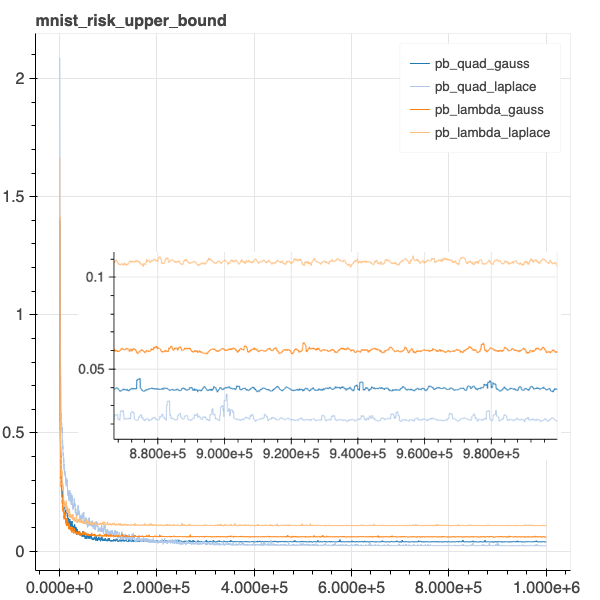
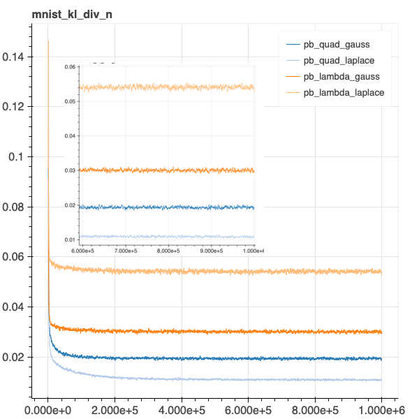
Figure 1: Objectives ‘pb_lambda’ and ‘pb_quad’ with Gauss and Laplace distributions. Plots for risk upper bound and normalized KL divergence ($\operatorname{KL}(Q\|Q^{0})/n_{\text{train}}$) vs training iterations for MNIST. The KL divergence starts at $0.0$, increases quickly and then starts decreasing later in the training.

6.1 The choice of the prior distribution

As pointed out above, our prior distributions (Laplace or Gauss) were centered at the randomly initialized weights. The attentive reader may object that, according to the usual PAC-Bayes theorems in the literature, priors are supposed to be non-random. To clarify, PAC-Bayes bounds require the prior to be a ‘data-free’ (i.e. non data-dependent) distribution. The randomness in the initialization of the weights is external to the training process, hence it is of the ‘data-free’ kind. This justifies that using priors centered at the randomly initialized weights is perfectly valid. Our choice of priors centred at the randomly initialized weights was motivated by observations of Zhang et al. [2019] indicating that post-training re-initialization of many weights has little effect on prediction performance. Subsequently we heard from Dziugaite and Roy [2017] that they used the same choice before.

6.2 Experiments on MNIST

For experiments on MNIST we trained a feed forward neural network with 3 hidden layers, with 600 units and ReLU activations in each hidden layer. We trained our models using standard MNIST dataset split of 50000 training examples and 10000 test examples. We ran all experiments for $1$ million training iterations. We observe from Fig. 2 that the methods converge around $100000$ iterations. We ran the experiments longer to check if the KL divergence can be minimized further. We used training batch size of $256$ for all the experiments.

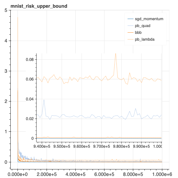
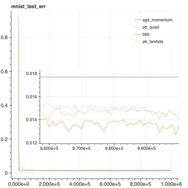
Figure 2: Plots for training objectives and test errors vs the training iterations for MNIST.

On Fig. 2 we report the test error and the risk upper bound as a function on the number of training iterations. Our methods ‘pb_lambda’ and ‘pb_quad’ achieve similar test accuracy at the end of training compared to BBB and SGD with momentum baseline. The $\eta$ parameter in BBB which is of $O(1\mathrm{e}-5)$ makes the KL divergence component of the loss insignificant compared to train loss. Thus in case of BBB we see marginal decrease in the KL divergence during the course of training and the solution it returns is expected to be similar to that returned with the SGD with momentum baseline. The best test error achieved by our methods 0.014 is comparable to the risk upper bound of 0.02 at the end of training. This is a significant improvement with respect to previously computed non-vacuous bounds. Also we note that for ‘pb_lambda’ method the $\lambda$ value start at $1$ and decreases to $0.5$ and starts increasing again after around $150000$ iterations to finally reach a value of $0.75$.

6.3 Comparison to Dziugaite and Roy [2018]

We are not the first to propose training methods or risk certificates for neural networks based on PAC-Bayes bounds. Langford and Caruana [2001] developed a method to train a stochastic neural network by randomizing the weights with Gaussian noise (adjusted via a sensitivity analysis) and computed an upper bound on the error using a PAC-Bayes bound. They run experiments on a UCI data set and a synthetic data set, and also pointed that the PAC-Bayes approach might be more fruitful for computing non-vacuous bounds. Dziugaite and Roy [2017] derived a training objective from a similar PAC-Bayes bound to train a stochastic neural network with Gaussian randomization, and computed non-vacuous bounds on a ‘Binary MNIST’ dataset. London [2017] approached the generalization of stochastic neural networks by a stability-based PAC-Bayes analysis, and run experiments on CIFAR-10. Other efforts showing further evidence in favour of the PAC-Bayes approach for neural networks are e.g. Neyshabur et al. [2017a, b], and Pitas et al. [2017].

Method	Test Error	Risk upper bound
Dziugaite and Roy [2018] ($\tau=3\mathrm{e}+3$)	0.12	0.21
Dziugaite and Roy [2018] ($\tau=1\mathrm{e}+5$)	0.06	0.65
Lever et al. [2013] ($\tau=3\mathrm{e}+3$)	0.12	0.26
Lever et al. [2013] ($\tau=1\mathrm{e}+5$)	0.06	1
PBB	0.014	0.023

Table 1: Test set error / Risk upper bound for standard MNIST dataset.

Usually, as we also noticed, the problem is that the KL term tends to dominate and most of the work in training is targeted at reducing it. To address this issue distribution-dependent (Lever et al. [2013]) or data-dependent (Dziugaite and Roy [2018]) priors can be used. The latter derived a novel PAC-Bayes bound under differentially private (or, distributionally stable) priors and proposed a procedure to minimize the terms in the bound in connection to training neural networks. While there is no fully rigorous argument for backing up their finite-time procedure, an asymptotic argument is available. What makes their work especially relevant to us is that they also provide results of experiments on standard multiclass MNIST. The values in Table 1 were reported by them. We compare our results (PBB) with the best value they achieved on the test error and risk upper bound.

The parameter $\tau$ in their setting controls the temperature of a Gibbs distribution. In the table we display only the two values of their $\tau$ parameter which achieve best test error and risk upper bound. Notice that our method did not use data-dependent priors, while Dziugaite and Roy [2018] used data-dependent priors. The rows ‘Lever et al. [2013]’ display values achieved by minimizing a PAC-Bayes bound that uses a different approach to relate the priors to the data, namely, the priors used by Lever et al. [2013] were distribution-dependent (see also Lever et al. [2010]). The method based on the PAC-Bayes bound of Lever et al. [2013] was implemented for neural networks by Dziugaite and Roy [2018] and used as a baseline to contrast the experimental results.

It is interesting to compare our results with the values obtained by other methods in table above. We note that Dziugaite and Roy [2018]’s best values correspond to test accuracy of 94% or 93% while in those cases their bound values, although non-vacuous, were far from tight. On the other hand the tightest value of their bound only gives an 88% accuracy. By contrast, our method PBB achieves close to 98.6% test accuracy (or 0.014 test error) even without using a data-dependent prior. At the same time, as noted above, our optimal upper bound value (0.023) is much tighter than theirs (0.21).

6.4 Comparison to Dziugaite and Roy [2017]

To compare our results with Dziugaite and Roy [2017]’s results we also run experiments on their ‘Binary MNIST’ dataset where digits $0-4$ were mapped to class $0$ and digits $5-9$ were mapped to class $1$. We implemented the network architecture which achieved the best test error in their setting.

Method	Test error	Risk upper bound
Dziugaite and Roy [2017]	0.013	0.201
PBB	0.015	0.022

Table 2: Test set error / Risk upper bound for ‘Binary MNIST’ dataset.

From the results in Table 2 we note that we achieve similar test set accuracy, while the minimal value of our risk upper bound is significantly tighter, i.e. our method PBB further tightens the gap between the risk certificate (upper bound) and the risk estimate evaluated on a test set.

7 Conclusion and Future Work

We explored the ‘PAC-Bayes with Backprop’ (PBB) methods to train probabilistic neural networks. The take-home message is that these training methods are derived from sound theoretical foundations, and output models that come with a performance guarantee at no extra cost, since PBB training objectives are based on PAC-Bayes bounds which upper bound the risk. This is an improvement over methods derived heuristically rather than from theoretically justified arguments, and over methods that do not include a risk certificate that is valid on unseen examples.

We presented two PBB training objectives. As far as we are aware, we are the first to use these objectives for neural network training. The results of our experiments on MNIST have showed that these two PBB objectives give predictors with competitive test set performance and with computed non-vacuous bounds that are significantly improved compared to previous results. This indicates that PBB methods look promising for achieving self-bounding learning, since the values of the risk certificates output by the training methods are close to the values of the test set error estimates. Additional experiments on some UCI data sets confirm these observations.

However, since the results of initial experiments on CIFAR-10 showed risk certificates with values not as close to the test set error estimate as in the MNIST or UCI experiments, more needs to be done before ‘self-bounding learning’ can really be claimed. We found that the biggest issue when using PBB is the KL term. In particular this is noticeable for larger networks. Besides the obvious choice of smaller networks, some ideas to deal with this issue in future work are e.g. coupling of weights to reduce the number of terms in the KL, using hierarchical priors (mixture over networks of different sizes), or using data-dependent priors. We believe that these combinations may have the chance of giving tight bounds and simultaneously achieving state-of-the-art test set performance.

Appendix A KL formulas: Laplace versus Gauss

The Laplace density with mean parameter $\mu\in\mathbb{R}$ and variance $b>0$ is the following:

$$p(x)=(2b)^{-1}\exp\bigl{(}-\frac{|x-\mu|}{b}\bigr{)}\,.$$

The KL divergence for two Laplace distributions is as follows:

$$\operatorname{KL}(\operatorname{Lap}(\mu_{1},b_{1})\|\operatorname{Lap}(\mu_{0},b_{0}))=\log(\frac{b_{0}}{b_{1}})+\frac{|\mu_{1}-\mu_{0}|}{b_{0}}+\frac{b_{1}}{b_{0}}e^{-|\mu_{1}-\mu_{0}|/b_{1}}-1\,.$$ (9)

For comparison, recall that the Gaussian density with mean parameter $\mu\in\mathbb{R}$ and variance $b>0$ has the following form:

$$p(x)=(2\pi b)^{-1/2}\exp\bigl{(}-\frac{(x-\mu)^{2}}{2b}\bigr{)}\,.$$

The KL divergence for two Gaussian distributions is as follows:

$$\operatorname{KL}(\operatorname{Gauss}(\mu_{1},\sigma_{1}^{2})\|\operatorname{Gauss}(\mu_{0},\sigma_{0}^{2}))=\frac{1}{2}\Bigl{(}\log(\frac{b_{0}}{b_{1}})+\frac{(\mu_{1}-\mu_{0})^{2}}{b_{0}}+\frac{b_{1}}{b_{0}}-1\Bigr{)}\,.$$ (10)

Appendix B Experiments on some UCI data sets

For experiments on UCI datasets we trained a feed forward neural network with ReLU activations in each hidden layer, with 64 units in the first hidden layer and 32 units in the second hidden layer, followed by an output layer. We performed experiments on 5 different UCI datasets. We ran all experiments for $30000$ training iterations. We used training batch size of $256$ for all the experiments.

UCI dataset	pb_lambda	pb_quad	bbb	sgd_momentum
MUSHROOM	0.0 / 0.0	0.0 / 0.0	0.0	0.0
BREAST	0.047 / 0.051	0.029 / 0.134	0.047	0.065
AvsB	0.0 / 0.013	0.0 / 0.052	0.0	0.0
IONOSPHERE	0.110 / 0.224	0.117 / 0.420	0.145	0.110
SKIN	0.001 / 0.001	0.001 / 0.001	0.002	0.002

Table 3: Test set error / Risk upper bound for UCI datasets.

In Table 3 we list the test error / risk upper bound for various methods. We note that both ‘pb_lambda’ and ‘pb_quad’ obtain similar test accuracy to that of BBB and SGD with momentum baselines. Also the risk upper bounds are comparable to the test errors. We would like to emphasize that BBB uses cross-validation over $\eta$ in Eq. 8 to obtain good performance, while ‘pb_lambda’ automatically tunes the coefficient $\lambda$ which controls the weight of the various components in the objective function.

References

- Blundell et al. [2015] Charles Blundell, Julien Cornebise, Koray Kavukcuoglu, and Daan Wierstra. Weight uncertainty in neural networks. In 32nd International Conference on Machine Learning, pages 1613–1622, 2015.
- Bottou [2012] Léon Bottou. Stochastic gradient descent tricks. In Neural networks: Tricks of the trade, pages 421–436. Springer, 2012.
- Boucheron et al. [2013] Stéphane Boucheron, Gábor Lugosi, and Pascal Massart. Concentration inequalities: A nonasymptotic theory of independence. Oxford university press, 2013.
- Caruana et al. [2001] Rich Caruana, Steve Lawrence, and C Lee Giles. Overfitting in neural nets: Backpropagation, conjugate gradient, and early stopping. In Advances in Neural Information Processing Systems, pages 402–408, 2001.
- Dua and Graff [2017] Dheeru Dua and Casey Graff. UCI Machine Learning Repository, 2017. URL http://archive.ics.uci.edu/ml.
- Dziugaite and Roy [2017] Gintare Karolina Dziugaite and Daniel M. Roy. Computing Nonvacuous Generalization Bounds for Deep (Stochastic) Neural Networks with Many More Parameters than Training Data. In UAI, 2017.
- Dziugaite and Roy [2018] Gintare Karolina Dziugaite and Daniel M Roy. Data-dependent PAC-Bayes priors via differential privacy. In Advances in Neural Information Processing Systems, pages 8430–8441, 2018.
- Freund [1998] Yoav Freund. Self bounding learning algorithms. In Proceedings of the eleventh annual conference on Computational Learning Theory, pages 247–258. ACM, 1998.
- Hinton and van Camp [1993] Geoffrey E Hinton and Drew van Camp. Keeping neural networks simple. In International Conference on Artificial Neural Networks, pages 11–18. Springer, 1993.
- Jankowiak and Obermeyer [2018] Martin Jankowiak and Fritz Obermeyer. Pathwise Derivatives Beyond the Reparameterization Trick. arXiv:1806.01851, 2018.
- Langford and Blum [2003] John Langford and Avrim Blum. Microchoice bounds and self bounding learning algorithms. Machine Learning, 51(2):165–179, 2003.
- Langford and Caruana [2001] John Langford and Rich Caruana. (Not) bounding the true error. In Advances in Neural Information Processing Systems, pages 809–816, 2001.
- Langford and Seeger [2001] John Langford and Matthias Seeger. Bounds for averaging classifiers. Technical Report CMU-CS-01-102, Carnegie Mellon University, 2001.
- Lever et al. [2010] Guy Lever, François Laviolette, and John Shawe-Taylor. Distribution-dependent PAC-Bayes priors. In International Conference on Algorithmic Learning Theory, pages 119–133. Springer, 2010.
- Lever et al. [2013] Guy Lever, François Laviolette, and John Shawe-Taylor. Tighter PAC-Bayes bounds through distribution-dependent priors. Theoretical Computer Science, 473:4–28, 2013.
- London [2017] Ben London. A PAC-Bayesian analysis of randomized learning with application to stochastic gradient descent. In Advances in Neural Information Processing Systems, pages 2931–2940, 2017.
- Maurer [2004] Andreas Maurer. A note on the PAC Bayesian theorem. arXiv:cs/0411099, 2004.
- Neal [1993] Radford M Neal. Bayesian Learning via Stochastic Dynamics. In Advances in Neural Information Processing Systems, pages 475–482, 1993.
- Neyshabur et al. [2017a] Behnam Neyshabur, Srinadh Bhojanapalli, David McAllester, and Nati Srebro. Exploring generalization in deep learning. In Advances in Neural Information Processing Systems, pages 5947–5956, 2017a.
- Neyshabur et al. [2017b] Behnam Neyshabur, Srinadh Bhojanapalli, and Nathan Srebro. A PAC-Bayesian approach to spectrally-normalized margin bounds for neural networks. arXiv:1707.09564, 2017b.
- Noy and Crammer [2014] Asaf Noy and Koby Crammer. Robust forward algorithms via PAC-Bayes and Laplace distributions. In Artificial Intelligence and Statistics, pages 678–686, 2014.
- Pitas et al. [2017] Konstantinos Pitas, Mike Davies, and Pierre Vandergheynst. PAC-Bayesian Margin Bounds for Convolutional Neural Networks. arXiv:1801.00171, 2017.
- Price [1958] Robert Price. A useful theorem for nonlinear devices having Gaussian inputs. IRE Transactions on Information Theory, 4(2):69–72, 1958.
- Seeger [2002] Matthias Seeger. PAC-Bayesian Generalization Error Bounds for Gaussian Process Classification. Journal of Machine Learning Research, 3:233–269, 2002.
- Shalev-Shwartz and Ben-David [2014] Shai Shalev-Shwartz and Shai Ben-David. Understanding Machine Learning. Cambridge University Press, Cambridge, 2014.
- Srivastava et al. [2014] Nitish Srivastava, Geoffrey Hinton, Alex Krizhevsky, Ilya Sutskever, and Ruslan Salakhutdinov. Dropout: a simple way to prevent neural networks from overfitting. Journal of Machine Learning Research, 15(1):1929–1958, 2014.
- Thiemann et al. [2017] Niklas Thiemann, Christian Igel, Olivier Wintenberger, and Yevgeny Seldin. A strongly quasiconvex PAC-Bayesian bound. In International Conference on Algorithmic Learning Theory, pages 466–492, 2017.
- Wan et al. [2013] Li Wan, Matthew Zeiler, Sixin Zhang, Yann Le Cun, and Rob Fergus. Regularization of neural networks using dropconnect. In International Conference on Machine Learning, pages 1058–1066, 2013.
- Zhang et al. [2019] Chiyuan Zhang, Samy Bengio, and Yoram Singer. Are All Layers Created Equal? arXiv:1902.01996, 2019.