Expected path length on random manifolds

Abstract

Manifold learning seeks a low dimensional representation that faithfully captures the essence of data. Current methods can successfully learn such representations, but do not provide a meaningful set of operations that are associated with the representation. Working towards operational representation learning, we endow the latent space of a large class of generative models with a random Riemannian metric, which provides us with elementary operators. As computational tools are unavailable for random Riemannian manifolds, we study deterministic approximations and derive tight error bounds on expected distances.
Key words: random fields, random metrics on manifolds, Gaussian process latent variable models, expected curve length.

1 Introduction

Manifold learning is one of the cornerstones of unsupervised learning. Classical methods such as Isomap [31], Locally linear embeddings [29], Laplacian eigenmaps [4] and more [30, 11] all seek a low dimensional embedding of high dimensional data that preserves prespecified aspects of data. Probabilistic methods often view the data manifold as governed by a latent variable along with a generative model that describes how the latent manifold is to be embedded in the data space. The common theme is the quest for a low dimensional representation that faithfully captures the data.

Ideally, we want an operational representation, that is we want to be able to make mathematically meaningful calculations with respect to the learned representation. It has been argued [17] that a good representation should at least support the following:

• Interpolation: given two points, a natural unique interpolating curve that follows the manifold should exist.

• Distances: the distance between two points should be well defined and informally reflect the amount of energy required to transform one point to another.

• Measure: the representation should be equipped with a measure under which integration is well defined for all points on the manifold.

These are elementary requirements of a representation, but most nonlinear manifold learning schemes do not imply or provide such operations.

In the sequel we will use the following notation. We denote by $Z$ the $d$-dimensional representation or latent space, which is learned from data in the observation space $X$. Latent points are denoted $z_{i}\in Z$, while corresponding observations are $x_{i}\in X$.

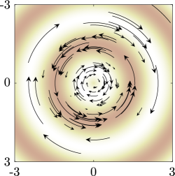
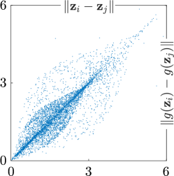
Figure 1: Reparametrizations illustrated. Left: A “swirling” transformation of the latent space $Z$. Right: Pair wise distances between points before and after reparametrization; clearly the Euclidean distances change with reparametrizations.

Embedding methods seek a low dimensional embedding $z_{1:N}=\{z_{1},\ldots,z_{N}\}\subset Z$ of the data $x_{1:N}\subset X$. These methods fundamentally only describe the data manifold at the points where data is observed and nowhere else. As such, the low dimensional embedding space is only well defined at $z_{1:N}$. It is common to treat the low dimensional embedding space as equipped with the Euclidean metric, but this is generally a post hoc assumption with limited grounding in the embedding method. Fundamentally, the learned representation space is a discrete space that does not lend itself to continuous interpolations. Likewise, the most natural measure will only assign mass to the points $z_{1:N}$, and any associated distribution will be discrete. It is not clear how this can naturally lead to an operational representation.

Generative models estimate a set of low dimensional latent variables $z_{1:N}$ along with a suitable mapping $f:Z\rightarrow X$ such that $f(z)\approx x$. It is, again, common to treat the latent space $Z$ together with the Euclidean metric. However, this assumption is unwarranted. As an example, consider the variational autoencoder (VAE) [22, 28], which seeks a representation in which $z_{1:N}$ follow a unit Gaussian distribution. Now consider a 2-dimensional latent space and the transformation $g(z)=R_{\theta}z$, where $R_{\theta}$ is a linear transformation that rotates points by $\theta(z)=\sin(\pi\|z\|)$. This is a smooth invertible transformation with the property that $z\sim\mathcal{N}(0,I)\Rightarrow g(z)\sim\mathcal{N}(0,I)$; see Fig. 1. If the latent variables $z_{1:N}$ and the mapping $f$ is an optimal VAE, then $g(z_{1:N})$ and $f\circ g^{-1}$ is equally optimal. Yet, the latent spaces $Z$ and $g(Z)$ are quite different; Fig. 1 shows the Euclidean distances between pairs of points of the latent space before and after applying $g$, for samples drawn from a unit Gaussian. Clearly, the transformed latent space is significantly different from the original space. As the VAE provides no guarantees as to which latent space is recovered, we must be careful when relying on the Euclidean latent space: distances between points are effectively arbitrary, as are straight line interpolations. Ideally, we want a representation that is invariant under such transformations, but current models do not have such properties.

In this paper, we consider probabilistic latent variable models on the form $x=f(z)$ where $f$ is a smooth stochastic process. The latent space can then be endowed with a random Riemannian metric to ensure that the learned latent representation is operational as defined above. We consider a deterministic approximation to the random Riemannian metric, and provide tight approximation bounds for expected distances (Proposition 4.6). The approximation is good when the data is high dimensional, which is often the case in machine learning applications. The analysis justifies the use of deterministic approximations, which in turn lead to computationally tractable algorithms.

The paper is structured to first provide a short primer on (deterministic) Riemannian geometry (Sec. 2). We then extend this class of geometries to the stochastic setting (Sec. 3), and provide our main theoretical contributions (Sec. 4) that analyze to which extend stochastic manifolds are well approximated by deterministic ones. Our analysis holds for any smooth stochastic generative process, which we exemplify (Sec. 5) with Gaussian process latent variable models [24].

2 Riemannian manifolds

A $d$-dimensional manifold $\mathcal{M}$ embedded in $\mathbb{R}^{n}$ with $d<n$ is a topological space in which each point $x\in\mathcal{M}$ has a neighborhood that is homeomorphic to $\mathbb{R}^{d}$ [15]. We may think of $\mathcal{M}$ as a smooth (nonlinear) surface in space that does not self intersect or change dimensionality. At each point $x\in\mathcal{M}\subseteq\mathbb{R}^{n}$ we have the tangent space $T_{x}\mathcal{M}$ of $\mathcal{M}$ at $x$ which may be seen as a linear approximation of $\mathcal{M}$ near $x$. In Fig. 2 a 2-dimensional manifold embedded in $\mathbb{R}^{3}$ is shown together with part of a tangent space.

Figure 2: Image of an embedded manifold $\mathcal{M}$ and the tangent space $T_{x}\mathcal{M}$ at a point $x\in\mathcal{M}$.

Let $f:Z\to\mathcal{M}\subseteq\mathbb{R}^{n}$ be a parametrization of an open subset $f(Z)\subseteq\mathcal{M}$ defined on some open subset $Z\subseteq\mathbb{R}^{d}$. A Riemannian metric on $Z$ is an inner product $\langle\cdot,\cdot\rangle_{z}$ on the tangent spaces $T_{z}Z\cong T_{z}\mathbb{R}^{d}$ which varies smoothly from point to point. Here, smooth means infinitely differentiable. Such a metric may be given by a positive definite $(d\times d)$-matrix $M_{z}$ which depends smoothly on $z\in Z$. The induced inner product is then $\langle v,w\rangle_{z}=v^{T}M_{z}w$ for $v,w\in T_{z}\mathbb{R}^{d}$ seen as column vectors.

Consider the standard inner product between points in $\mathbb{R}^{n}$, $\langle x,x^{\prime}\rangle=\sum_{i=1}^{n}x_{i}x_{i}^{\prime}$ where $x=(x_{1},\dots,x_{n})$ and $x^{\prime}=(x_{1}^{\prime},\dots,x_{n}^{\prime})$. Let $z\in Z$ and let $\Delta_{1},\Delta_{2}\in U\subset\mathbb{R}^{d}$ where $U$ is an open ball centered at the origin such that $z+U\subseteq Z$. Then we can compute the inner product of $\Delta_{1}$ and $\Delta_{2}$ at $z$ using the Taylor expansion of $f$. Consider the scalar product $\langle f(z+\Delta_{1})-f(z),f(z+\Delta_{2})-f(z)\rangle$, and the linear part of it in $\Delta_{1}$ and $\Delta_{2}$ which we denote by $\langle f(z+\Delta_{1})-f(z),f(z+\Delta_{2})-f(z)\rangle_{0}$. Then

$$\langle f(z+\Delta_{1})-f(z),f(z+\Delta_{2})-f(z)\rangle_{0}=$$

$$\langle f(z)+J_{f}(z)\Delta_{1}-f(z),f(z)+J_{f}(z)\Delta_{2}-f(z)\rangle=$$

$$\langle J_{f}(z)\Delta_{1},J_{f}(z)\Delta_{2}\rangle=\Delta_{1}^{\top}J_{f}(z)^{\top}\mkern-1.5muJ_{f}(z)\Delta_{2},$$

where $J_{f}(z)$ is the $n\times d$ Jacobian matrix of $f$ at $z$. The $d\times d$ symmetric positive definite matrix $M_{z}=J_{f}(z)^{\top}\mkern-1.5muJ_{f}(z)$ defines a Riemannian metric on $Z$ induced by $f$ which is called the pullback metric. Note that the pullback metric corresponds to the Riemannian metric on $\mathcal{M}$ induced by the inner product in the ambient space $\mathbb{R}^{n}$, which does not depend on the choice of parametrization $f$. In this way, the pullback metric avoids the parametrization issue discussed in the opening section.

Distances & interpolants. The length of a smooth curve $c:[a,b]\rightarrow Z$ under the local inner product is

$$\mathcal{L}(c)=\int_{a}^{b}\sqrt{\dot{c}_{t}^{\top}M_{c_{t}}\dot{c}_{t}}\mathrm{d}t,$$

where $c_{t}=c(t)$ and $\dot{c}_{t}=\partial_{t}c(t)$ is the curve and its derivative, respectively. Natural interpolants (geodesics) can then be defined as length minimizing curves connecting two points. The length of such a curve is a natural distance measure along the manifold. Unfortunately, minimizing curve length gives rise to a poorly determined optimization problem as the length of a curve is independent of the parametrization. The following proposition provides remedy [15]:

Proposition 2.1.

Let $c:[a,b]\rightarrow Z$ be a smooth curve that (locally) minimizes the curve energy

$$\mathcal{E}(c) =\frac{1}{2}\int_{a}^{b}\dot{c}_{t}^{\top}M_{c_{t}}\dot{c}_{t}\mathrm{d}t.$$ (1)

Then $c$ has constant velocity and is locally length-minimizing.

Integration. Given a function $h:\mathbb{R}^{n}\rightarrow\mathbb{R}$ and an open subset $\Omega\subseteq Z$ we can integrate $h$ over $f(\Omega)$ as [26]

$$\int_{f(\Omega)}h(x)\mathrm{d}x =\int_{\Omega}h(f(z))\sqrt{\det(M_{z})}\mathrm{d}z.$$

The quantity $\sqrt{\det(M_{z})}$ is known as the Riemannian volume measure and is akin to the Jacobian determinant in the change of variables theorem.

Relation to latent variable models. As stated in the introduction, we are concerned with latent variable models $x=f(z)$, where $f$ is a smooth stochastic process. The above constructions assume that $f$ is deterministic. In this case, Riemannian geometry provides us with the tools to make the representation operational as defined in the introduction. This paper is concerned with extending Riemannian geometry to the stochastic domain in order to provide operational representations in latent variable models. To make the resulting constructions practical, we will further show how the stochastic geometry can be approximated well by deterministic geometries that lend themselves to computations.

3 Stochastic Riemannian geometry

In this section we establish the basic definitions in the area of random manifolds. To the best of our knowledge this is a fairly unexplored topic and in our opinion it deserves more attention. Related work has been done in the area of random fields, see for instance [1]. To illustrate the concepts the definitions are followed by some elementary examples.

We start by defining random metrics.

Definition 3.1.

Let $Z\subseteq\mathbb{R}^{d}$ be an open subset. A random (or stochastic) Riemannian metric is a matrix-valued random field on $Z$ whose sample paths are Riemannian metrics. We also refer to $Z$ equipped with the random metric as a random manifold.

The stochastic Riemannian metrics considered in this paper are induced by a stochastic process $f:Z\to\mathbb{R}^{n}$ for some $n$, where $Z\subseteq\mathbb{R}^{d}$ is an open subset. More precisely, $f$ is a random field in the sense of [1]. In our examples we will have $Z=\mathbb{R}^{d}$ but it is useful to keep in mind that the parametrization may not be defined on the whole of $\mathbb{R}^{d}$. Now, in order for $f$ to induce a random metric it must satisfy some differentiability conditions. One option is to require that any sample path from $f$ is smooth. In that case we say that $f$ is smooth. If in addition the sample paths $s:Z\to\mathbb{R}^{n}$ are such that the Jacobian matrix $J_{s}$ has full rank everywhere, $f$ is called a stochastic immersion. This implies that $s$ is locally injective and that $s(Z)\subseteq\mathbb{R}^{n}$ is an immersed submanifold. A stochastic immersion whose sample paths are injective is called a stochastic embedding. In this case the sample paths $s:Z\to\mathbb{R}^{n}$ are embedded submanifolds $s(Z)\subseteq\mathbb{R}^{n}$. As such, $s(Z)$ has an induced Riemannian metric from the ambient space $\mathbb{R}^{n}$ and this defines a stochastic Riemannian metric on $Z$. Another point of view of the basic objects is thus as random embedded submanifolds of $\mathbb{R}^{n}$. These submanifolds all have the same constant topology and smooth structure induced by $Z$ and hence from an intrinsic point of view, the random aspect of these manifolds is confined to the Riemannian metric. If the conditions to be a stochastic immersion or embedding are only true with probability 1 we can modify the process by restricting to the measure 1 subset of the probability space where the requirements are fulfilled.

As in the deterministic case, the metric on $Z$ induced by $f$ is given by the pullback metric

$$M=J_{f}^{T}J_{f},$$

where $J_{f}$ is the Jacobian of $f$. In accordance with the definition of stochastic Riemannian metrics, $M$ is a matrix-valued stochastic process parametrized by $Z$.

If it exists, we may also consider the expected metric on $Z$ which is given by the mean value $\mathbb{E}(M)=\mathbb{E}(J_{f}^{T}J_{f})$.

Definition 3.2.

Let $f:Z\to\mathbb{R}^{n}$ be a stochastic immersion such that all the entries of the matrix $\mathbb{E}(M)=\mathbb{E}(J_{f}^{T}J_{f})$ are finite smooth functions. We then refer to $\mathbb{E}(M)$ as the expected metric. It defines a Riemannian metric on $Z$ making it into a Riemannian manifold which is called the mean manifold.

Note that the mean manifold is typically not given by the mean value of $f$, that is the map $\mathbb{E}(f):Z\to\mathbb{R}^{n}:z\mapsto\mathbb{E}(f(z))$. The expected metric has been previously studied for the Gaussian process latent variable model [32], and the variational autoencoder [2].

Remark 3.3.

The requirement that a stochastic process $f:Z\to\mathbb{R}^{n}$ has smooth sample paths with probability 1 is not always straightforward to verify. An alternative assumption that is relatively easy to check is that $f$ is differentiable in mean square, see [1]. We say that $f$ is mean square smooth if $f$ has mean square derivatives of any order. Let $J_{f}$ denote the mean square Jacobian of a mean square smooth process with smooth covariance function. The expected metric may be considered in this setting as well, assuming that $\mathbb{E}(M)=\mathbb{E}(J_{f}^{T}J_{f})$ has full rank. The main result of this paper, Proposition 4.6, compares expected length on random manifolds to length in the expected metric. This result holds both in the smooth and mean square smooth setting.

Example 3.4.

A significant special case is a Gaussian process or Gaussian random field

$$f:\mathbb{R}^{d}\to\mathbb{R}^{n}:q\mapsto(f_{1}(q),\dots,f_{n}(q)),$$

with $d\leq n$. Here, the components $f_{i}:\mathbb{R}^{d}\to\mathbb{R}$ are Gaussian processes, which means that the vector $(f_{i}(q_{1}),\dots,f_{i}(q_{r}))$ is Gaussian for any $q_{1},\dots,q_{r}\in\mathbb{R}^{d}$. In fact, that $f:\mathbb{R}^{d}\to\mathbb{R}^{n}$ is a Gaussian process means that $\sum_{i=1}^{n}\alpha_{i}f_{i}$ is a Gaussian process for all $\alpha_{1},\dots,\alpha_{n}\in\mathbb{R}$. We will be concerned with the case where the random vectors $(f_{i}(q_{1}),\dots,f_{i}(q_{r}))$ and $(f_{j}(q_{1}),\dots,f_{j}(q_{r}))$ are independent for $i\neq j$ and all $q_{1},\dots,q_{r}\in\mathbb{R}^{d}$. The distribution of $(f_{i}(q_{1}),\dots,f_{i}(q_{r}))$ is determined by the mean function $\mu_{i}:\mathbb{R}^{d}\to\mathbb{R}:p\mapsto\mathbb{E}(f_{i}(p))$ and the covariance function $k_{i}:\mathbb{R}^{d}\times\mathbb{R}^{d}\to\mathbb{R}:(p,q)\mapsto\mathbb{E}((f_{i}(p)-\mu_{i}(p))(f_{i}(q)-\mu_{i}(q)))$. If $k_{i}$ and $\mu_{i}$ are real analytic functions, then $f_{i}$ is mean square smooth. This can be seen from the criterion (1.4.9) in [1]. Moreover, for any column vector $v\in\mathbb{R}^{d}$,

$$v^{T}\mathbb{E}(J_{f}^{T}J_{f})v=\mathbb{E}(v^{T}J_{f}^{T}J_{f}v)=\mathbb{E}(||J_{f}v||^{2})=\sum_{i=1}^{n}\mathbb{E}(\nabla f_{i}\cdot v)^{2}+\sum_{i=1}^{n}\operatorname{var}(\nabla f_{i}\cdot v),$$

and $\mathbb{E}(\nabla f_{i}\cdot v)=\nabla\mu_{i}\cdot v$. Hence $\mathbb{E}(J_{f}^{T}J_{f})$ has full rank for example if $\mu=(\mu_{1},\dots,\mu_{n})$ is locally injective or $\nabla f_{i}$ has non-degenerate covariance matrix for some $i$.

For Gaussian processes in machine learning, see [24, 27, 32] and in particular the Gaussian process latent variable model.

Example 3.5.

Another special case to keep in mind which is particularly simple is a stochastic embedding $f(x)=L(g(x))$, where $g:\mathbb{R}^{d}\to\mathbb{R}^{m}$ a deterministic smooth injection and $L:\mathbb{R}^{m}\to\mathbb{R}^{n}$ is a random matrix with $n\leq m$. Consider the case where $L$ is given by a distribution on $\operatorname{SO}(\mathbb{R}^{m},\mathbb{R}^{n})$, that is any sample of $L$ has orthonormal rows. Let $W$ be the span of the rows of $L$ and fix coordinates on $W$ given by the rows of $L$ as a basis. In this way, $f$ can be seen as a random projection of the deterministic manifold $g(\mathbb{R}^{d})\subseteq\mathbb{R}^{m}$ into $W$. Note that if $n<m$, this can be viewed as random dimensionality reduction. See [7] for a survey on the topic of random projections in machine learning. In this context it is relevant to recall the Johnson-Lindenstrauss lemma. Roughly speaking, given a finite set $E\subset\mathbb{R}^{m}$, distances in $E$ are well preserved by a random projection $\mathbb{R}^{m}\to\mathbb{R}^{n}$ if $n$ is big enough. See for example [10] for background on the Johnson-Lindenstrauss lemma. In the same spirit one can show that distances along the submanifold $g(\mathbb{R}^{d})\subseteq\mathbb{R}^{m}$ are well preserved under similar circumstances [3, 8, 14, 19, 23, 33].

Example 3.6.

Consider a simple random manifold given by a stochastic embedding

$$f:\mathbb{R}^{d}\to\mathbb{R}^{n}:z\mapsto(f_{1}(z),\dots,f_{n}(z)),$$

where $f_{i}=\mu_{i}+\epsilon_{i}\sigma_{i}$ for smooth functions $\mu_{i},\sigma_{i}:\mathbb{R}^{d}\to\mathbb{R}$ and random variables $\epsilon_{i}$ with $\mathbb{E}(\epsilon_{i})=0$ and $\mathbb{E}(\epsilon_{i}^{2})=1$. Let $\mu:\mathbb{R}^{d}\to\mathbb{R}^{n}:z\mapsto(\mu_{1}(z),\dots,\mu_{n}(z))$, $\sigma:\mathbb{R}^{d}\to\mathbb{R}^{n}:z\mapsto(\sigma_{1}(z),\dots,\sigma_{n}(z))$ and define

$$e=\begin{pmatrix}\epsilon_{1}&0&0&\ldots&0\\ 0&\epsilon_{2}&0&\ldots&0\\ &&\vdots&\\ 0&0&0&\ldots&\epsilon_{n}\end{pmatrix}.$$

Then $f=\mu+e\sigma$, where the product $e\sigma$ is matrix multiplication and $\mu$ and $\sigma$ are viewed as column vectors. Note that $\mathbb{E}(e)=0$ and $\mathbb{E}(e^{2})=\operatorname{Id}_{\mathbb{R}^{n}}$, that is $\mathbb{E}(e)$ is the zero matrix and $\mathbb{E}(e^{2})$ the identity matrix on $\mathbb{R}^{n}$. For the Jacobian of $f$ we get $J_{f}=J_{\mu}+eJ_{\sigma}$ and hence

$$M=J_{f}^{T}J_{f}=(J_{\mu}+eJ_{\sigma})^{T}(J_{\mu}+eJ_{\sigma})=J_{\mu}^{T}J_{\mu}+J_{\mu}^{T}eJ_{\sigma}+J_{\sigma}^{T}eJ_{\mu}+J_{\sigma}^{T}e^{2}J_{\sigma}.$$

Therefore $\mathbb{E}(J_{f}^{T}J_{f})=J_{\mu}^{T}J_{\mu}+J_{\mu}^{T}\mathbb{E}(e)J_{\sigma}+J_{\sigma}^{T}\mathbb{E}(e)J_{\mu}+J_{\sigma}^{T}\mathbb{E}(e^{2})J_{\sigma}=J_{\mu}^{T}J_{\mu}+J_{\sigma}^{T}J_{\sigma}$. This is also the metric on $\mathbb{R}^{d}$ induced by the embedding $g:\mathbb{R}^{d}\to\mathbb{R}^{2n}=\mathbb{R}^{n}\times\mathbb{R}^{n}$ given by

$$g:\mathbb{R}^{d}\to\mathbb{R}^{n}\times\mathbb{R}^{n}:z\mapsto(\mu(z),\sigma(z)).$$

The metric induced by $g$ has been studied empirically for variational autoencoders [2]. We see in this example how the mean manifold $g(\mathbb{R}^{d})\subseteq\mathbb{R}^{2n}$ depends on both the mean value $\mu=\mathbb{E}(f)$ and the standard deviation map $\sigma$.

Another point of view is that $f=L\circ g$ where

$$L=(\operatorname{Id}_{\mathbb{R}^{n}}|\;e)$$

is the random $(n\times 2n)$-matrix given by stacking the columns of the matrices $\operatorname{Id}_{\mathbb{R}^{n}}$ and $e$ side by side. This is a special case of the random manifolds considered in Ex. 3.5. In connection with Ex. 3.7 below we note that $\mathbb{E}(L^{T}L)=\operatorname{Id}_{\mathbb{R}^{2n}}$.

Example 3.7.

Recall Ex. 3.5 and random manifolds given by $f=L\circ g$ where $g:\mathbb{R}^{d}\to\mathbb{R}^{m}$ is an embedding and $L:\mathbb{R}^{m}\to\mathbb{R}^{n}$ is a random matrix. Assume that $\mathbb{E}(L^{T}L)$ has finite entries and full rank. We shall see that, similarly to Ex. 3.6, the mean manifold is essentially the manifold $g(\mathbb{R}^{d})\subseteq\mathbb{R}^{m}$. Since $\mathbb{E}(L^{T}L)$ is symmetric we may diagonalize $\mathbb{E}(L^{T}L)$ with an orthogonal $(m\times m)$-matrix $P$, that is $\mathbb{E}(L^{T}L)=P^{T}DP$ where $D$ is diagonal. Since $\mathbb{E}(L^{T}L)$ is positive definite we can take the square roots of the eigenvalues on the diagonal of $D$ to obtain a diagonal matrix $\sqrt{D}$. In this case the stochastic metric is $M=J_{f}^{T}J_{f}=J_{g}^{T}L^{T}LJ_{g}$ and the mean metric is $\mathbb{E}(M)=J_{g}^{T}\mathbb{E}(L^{T}L)J_{g}$. Hence the mean manifold is induced by the embedding $\mathbb{R}^{d}\to\mathbb{R}^{m}:z\mapsto\sqrt{D}Pg(z)$, which is just the manifold $g(\mathbb{R}^{d})\subseteq\mathbb{R}^{m}$ up to a change of coordinates. In contrast consider $\mathbb{E}(f):\mathbb{R}^{d}\to\mathbb{R}^{n}$, and note that $\mathbb{E}(f)=\mathbb{E}(L)\circ g$. The image of $\mathbb{E}(f)$ is thus the image of the embedded mean manifold $\sqrt{D}Pg(\mathbb{R}^{d})\subseteq\mathbb{R}^{m}$ under the linear map $\mathbb{E}(L)(\sqrt{D}P)^{-1}:\mathbb{R}^{m}\to\mathbb{R}^{n}$.

3.1 Expected length versus the expected metric

Let $Z\subseteq\mathbb{R}^{d}$ be an open subset. We will now explore the topic of shortest paths on a random manifold induced by a stochastic immersion $f:Z\to\mathbb{R}^{n}$ with expected metric $\mathbb{E}(M)$. In order to talk about expected length of curves on the random manifold we need that $f$ is measurable when viewed as a map $\Omega\times Z\to\mathbb{R}^{n}$, where $\Omega$ is a probability space. Here, $Z$ and $\mathbb{R}^{n}$ are endowed with the Lebesgue measure and $\Omega\times Z$ with the product measure. Now let $c:[a,b]\rightarrow Z$ denote a smooth immersed curve and consider its stochastic immersion $f\circ c$ in $\mathbb{R}^{n}$. We stress that $c$ is a deterministic curve in $Z$, while $f\circ c$ is a random curve in $\mathbb{R}^{n}$. The energy of $c$, defined as in Eq. 1, is a random quantity and it is natural to consider its expectation with respect to the random metric. Since the energy integrand is positive, Tonelli’s Theorem tells us that the expected energy $\epsilon(c)$ is given by

$$\epsilon(c) =\mathbb{E}(\mathcal{E}(c))=\frac{1}{2}\mathbb{E}\left(\int_{a}^{b}\dot{c}_{t}^{\top}M_{c_{t}}\dot{c}_{t}\mathrm{d}t\right)$$

$$=\frac{1}{2}\int_{a}^{b}\dot{c}_{t}^{\top}\mathbb{E}(M_{c_{t}})\dot{c}_{t}\mathrm{d}t.$$

This implies that a curve $c$ with minimal expected energy over the stochastic manifold is a geodesic under the deterministic Riemannian metric $\mathbb{E}(M)$.

We can understand a curve with minimal expected energy in more explicit terms as follows. Let $u_{t}=\mathbb{E}(\|\dot{c}_{t}\|)$ and $v_{t}=1$ denote two functions over the interval $[a,b]$; here we use the shorthand notation $\|\dot{c}_{t}\|=\sqrt{\dot{c}_{t}^{\top}M_{c_{t}}\dot{c}_{t}}$. The Cauchy-Schwartz inequality then gives

$$\left(\int_{a}^{b}\mathbb{E}(\|\dot{c}_{t}\|)\mathrm{d}t\right)^{2} \leq\int_{a}^{b}\mathbb{E}(\|\dot{c}_{t}\|)^{2}\mathrm{d}t\cdot\int_{a}^{b}\mathrm{d}t$$

$$=(b-a)\int_{a}^{b}\mathbb{E}(\|\dot{c}_{t}\|)^{2}\mathrm{d}t.$$

Let $l(c)\!=\!\mathbb{E}(\mathcal{L}(c))$ denote the expected length of $c$. Then

$$\int_{a}^{b}\mathbb{E}(\|\dot{c}_{t}\|)^{2}\mathrm{d}t \geq\frac{l^{2}(c)}{b-a}.$$ (2)

Equality is achieved when $u_{t}$ and $v_{t}$ are parallel, that is when $\mathbb{E}(\|\dot{c}_{t}\|)$ is constant. If the curve is regular in the sense that the expected speed $\mathbb{E}(\|\dot{c}_{t}\|)$ is non-zero for all $t$, then we can always reparametrize $c_{t}$ to have constant expected speed and achieve equality in Eq. 2. Since $\operatorname{var}(\|\dot{c}_{t}\|)=\mathbb{E}(\|\dot{c}_{t}\|^{2})-\mathbb{E}(\|\dot{c}_{t}\|)^{2}$, we see that

$$\int_{a}^{b}\!\mathbb{E}(\|\dot{c}_{t}\|)^{2}\mathrm{d}t =\int_{a}^{b}\!\mathbb{E}(\|\dot{c}_{t}\|^{2})\mathrm{d}t-\int_{a}^{b}\operatorname{var}(\|\dot{c}_{t}\|)\mathrm{d}t$$

$$=2\epsilon(c)-\int_{a}^{b}\operatorname{var}(\|\dot{c}_{t}\|)\mathrm{d}t.$$

Assuming that the curve has constant expected speed, we then get

$$\epsilon(c) =\frac{l^{2}(c)}{2(b-a)}+\frac{1}{2}\int_{a}^{b}\operatorname{var}(\|\dot{c}_{t}\|)\mathrm{d}t.$$

Minimizing expected curve energy, thus, does not always minimize the expected curve length. Rather, this balances the minimization of expected curve length and the minimization of curve variance.

4 Expected length in high codimension

Let $Z\subseteq\mathbb{R}^{d}$ be an open subset and $f:Z\to\mathbb{R}^{n}$ a stochastic immersion with expected metric $\mathbb{E}(M)$. Any smooth curve $c:[0,1]\to Z$ gives rise to a random curve $f\circ c:[0,1]\to\mathbb{R}^{n}$. In this section we continue to examine the relationship between the expected length of random curves and the length with respect to the expected metric. More precisely, we show that length with respect to the expected metric is a good approximation for expected length in high ambient dimension $n$. Assuming independence of the components of $f\circ c$ we could apply a version of the central limit theorem such as the Berry-Esseen theorem to this problem, see for example [12]. We found it more convenient to take a direct approach via the Taylor expansion of the norm of velocity vectors. See also [21, 5] and Chapter 27 of [9] for approximation results in the same vein.

4.1 Expected norm of high dimensional vectors

We will consider a sequence $W_{n}$ of random vectors in $\mathbb{R}^{n}$. This means that for each integer $1\leq n$ we have an $\mathbb{R}^{n}$-valued random variable $W_{n}$. Consider the norm $w_{n}=||W_{n}||$. Assume that $w_{n}^{2}$ has first and second moments and put $m_{n}=\sqrt{\mathbb{E}(w_{n}^{2})}$ and $\Sigma_{n}=\sqrt{n\cdot\operatorname{var}(w_{n}^{2})}$. We say that $m_{n}$ is bounded away from 0 if there is a constant $0<b$ such that $b<m_{n}$ for all $n$. For $1\leq k$, let $\mu_{k}(w_{n}^{2})=\mathbb{E}((w_{n}^{2}-m_{n}^{2})^{k})$ denote the $k$-th central moment of $w_{n}^{2}$.

Definition 4.1.

We call a sequence $W_{n}$ as above balanced if $m_{n}$ is bounded away from 0 and $m_{n}$, $n^{2}\mu_{3}(w_{n}^{2})$ and $n^{2}\mu_{4}(w_{n}^{2})$ are bounded sequences.

Suppose that $W_{n}$ is balanced. We shall see that $\Sigma_{n}$ is a bounded sequence. Let $Z_{n}=n(w_{n}^{2}-m_{n}^{2})^{2}$ and let $\mathcal{X}_{n}$ be the indicator function for the event $\{Z_{n}<1\}$. We know that $\mathbb{E}(Z_{n}^{2})=n^{2}\mu_{4}(w_{n}^{2})$ is bounded and need to show that $n\mu_{2}(w_{n}^{2})=\mathbb{E}(Z_{n})$ is bounded. This follows from $\mathbb{E}(Z_{n})\leq 1+\mathbb{E}(Z_{n}(1-\mathcal{X}_{n}))\leq 1+\mathbb{E}(Z_{n}^{2})$.

Remark 4.2.

Consider the cubic Taylor polynomial of $\sqrt{x}$ around $x=1$, $P(x)=1+\frac{1}{2}(x-1)-\frac{1}{8}(x-1)^{2}+\frac{1}{16}(x-1)^{3}$. We will show that $|\sqrt{x}-P(x)|\leq\frac{5}{16}(x-1)^{4}$ for all $x\geq 0$. Let $y=\sqrt{x}$ and put $Q(y)=P(y^{2})-y$. Since $16Q(y)=(y-1)^{4}(y^{2}+4y+5)$, we have that $Q(y)\geq 0$ for $y\geq 0$. Hence $P(x)-\sqrt{x}\geq 0$ for $x\geq 0$. Let $R(y)=\frac{5}{16}(y^{2}-1)^{4}-P(y^{2})+y$. Since $16R(y)=y(y-1)^{4}(5y^{3}+20y^{2}+29y+16)\geq 0$ for $y\geq 0$, we have that $\frac{5}{16}(x-1)^{4}\geq P(x)-\sqrt{x}$ for $x\geq 0$.

Proposition 4.3.

Let $W_{n}$ be a balanced sequence of vectors. Then

$$\mathbb{E}(w_{n})=m_{n}-\frac{\Sigma_{n}^{2}}{8n\cdot m_{n}^{3}}+\mathcal{O}(n^{-2}).$$

Proof.

We will first prove the statement assuming that $m_{n}=1$ for all $n$. In this case we need to show that $\mathbb{E}(w_{n})-(1-\Sigma_{n}^{2}/8n)=\mathcal{O}(n^{-2})$. Let $P(x)=1+\frac{1}{2}(x-1)-\frac{1}{8}(x-1)^{2}+\frac{1}{16}(x-1)^{3}$ be the cubic Taylor polynomial of $\sqrt{x}$ around $x=1$ and note that $\mathbb{E}(P(w_{n}^{2}))=1-\Sigma_{n}^{2}/8n+\frac{1}{16}\mu_{3}(w_{n}^{2})$. Since by assumption $\mu_{3}(w_{n}^{2})=\mathcal{O}(n^{-2})$, it is enough to show that $\mathbb{E}(w_{n})-\mathbb{E}(P(w_{n}^{2}))=\mathcal{O}(n^{-2})$. Note that

$$|\mathbb{E}(w_{n})-\mathbb{E}(P(w_{n}^{2}))|=|\mathbb{E}(w_{n}-P(w_{n}^{2}))|\leq\mathbb{E}(|w_{n}-P(w_{n}^{2})|).$$

Also, $|\sqrt{x}-P(x)|\leq\frac{5}{16}(x-1)^{4}$ for all $x\geq 0$ by Remark 4.2. Hence $|w_{n}-P(w_{n}^{2})|\leq(w_{n}^{2}-1)^{4}$ and by assumption we have $\mathbb{E}((w_{n}^{2}-1)^{4})=\mathcal{O}(n^{-2})$. It follows that $\mathbb{E}(|w_{n}-P(w_{n}^{2})|)\leq\mathbb{E}((w_{n}^{2}-1)^{4})=\mathcal{O}(n^{-2})$.

Now consider the general case of a balanced sequence $W_{n}$ and let $m_{n}$ and $\Sigma_{n}$ denote the corresponding sequences associated to $W_{n}$. Since $W_{n}/m_{n}$ is balanced, $\mathbb{E}(||W_{n}/m_{n}||^{2})=1$ for all $n$ and $n\cdot\operatorname{var}(||W_{n}/m_{n}||^{2})=\Sigma_{n}^{2}/m_{n}^{4}$, we have by above that

$$\mathbb{E}(w_{n}/m_{n})=1-\frac{\Sigma_{n}^{2}/m_{n}^{4}}{8n}+\mathcal{O}(n^{-2}).$$

But $m_{n}$ is bounded and so the claim follows by multiplying by $m_{n}$. ∎

Remark 4.4.

Suppose that $W_{n}$ is balanced. Since $\Sigma_{n}$ is bounded and $m_{n}$ bounded away from 0 we have that $\limsup_{n\to\infty}\Sigma_{n}<\infty$ and $\liminf_{n\to\infty}m_{n}>0$. Let $A,b\in\mathbb{R}$ be such that $A>\limsup_{n\to\infty}\Sigma_{n}$ and $0<b<\liminf_{n\to\infty}m_{n}$. Then, by Proposition 4.3,

$$0\leq m_{n}-\mathbb{E}(w_{n})\leq\frac{A^{2}}{8n\cdot b^{3}},$$ (3)

for large enough $n$. In particular, if $\Sigma_{n}\to\Sigma$ and $m_{n}\to m$ with $\Sigma,m\in\mathbb{R}$, then Eq. 3 holds for any $A>\Sigma$ and $0<b<m$. In this case we also have that

$$\lim_{n\to\infty}\mathbb{E}(w_{n})=\lim_{n\to\infty}m_{n}$$ (4)

and Proposition 4.3 gives some additional information concerning the rate of convergence. Note also that $\operatorname{var}(w_{n})=m_{n}^{2}-\mathbb{E}(w_{n})^{2}\to 0$ for balanced $W_{n}$.

4.2 Normed sequences of independent random variables

For $k\geq 1$ and a random variable $Y$ with first moment $\mathbb{E}(Y)$, let $\mu_{k}(Y)=\mathbb{E}((Y-\mathbb{E}(Y))^{k})$ denote the $k$-th central moment. Now consider a sequence $X_{1},X_{2},\dots$ of independent random variables and let

$$W_{n}=(X_{1}/\sqrt{n},\dots,X_{n}/\sqrt{n})$$

be the corresponding normalized sequence of vectors. We say that the sequence $X_{1},X_{2},\dots$ has bounded moments if the moments $\mathbb{E}(X_{i}^{k})$ form a bounded sequence for any $k\geq 1$. This implies that the central moments $\mu_{k}(X_{i})$ are bounded as well. Let $w_{n}=||W_{n}||$. The definition of a balanced sequence of vectors $W_{n}$ is motivated by this setup since, for instance, in this case $m_{n}^{2}=\mathbb{E}(w_{n}^{2})=\frac{1}{n}\sum_{i=1}^{n}\mathbb{E}(X_{i}^{2})$ is bounded if the sequence $X_{1},X_{2},\dots$ has bounded moments. Similarly, $\Sigma_{n}^{2}=n\cdot\operatorname{var}(w_{n}^{2})=n\cdot\frac{1}{n^{2}}\sum_{i=1}^{n}\operatorname{var}(X_{i}^{2})$ is bounded in this case.

Lemma 4.5.

Let $X_{1},X_{2},\dots$ be independent with bounded moments. If $m_{n}$ is bounded away from 0 then $W_{n}=(X_{1}/\sqrt{n},\dots,X_{n}/\sqrt{n})$ is balanced.

Proof.

We need to show that $n^{2}\mu_{3}(w_{n}^{2})$ and $n^{2}\mu_{4}(w_{n}^{2})$ are bounded. Note that $n^{2}\mu_{3}(w_{n}^{2})=n^{2}\mu_{3}(\frac{1}{n}\sum_{i=1}^{n}X_{i}^{2})=\frac{1}{n}\sum_{i=1}^{n}\mu_{3}(X_{i}^{2})$, which is bounded. Similarly,

$$n^{2}\mu_{4}(w_{n}^{2})=\frac{1}{n^{2}}\mu_{4}(\sum_{i=1}^{n}X_{i}^{2})=\frac{1}{n^{2}}\sum_{i=1}^{n}\mu_{4}(X_{i}^{2})+\frac{6}{n^{2}}\sum_{i<j}\mu_{2}(X_{i}^{2})\mu_{2}(X_{j}^{2}),$$

which is bounded as well. ∎

4.3 Expected length of curves

Consider a sequence of stochastic processes $f_{1},f_{2},\dots$ defined on $[0,1]$ such that for any $t\in[0,1]$, $f^{\prime}_{1}(t),f^{\prime}_{2}(t),\dots$ are independent. Let

$$\phi_{n}:[0,1]\to\mathbb{R}^{n}:t\mapsto(f_{1}(t)/\sqrt{n},\dots,f_{n}(t)/\sqrt{n})$$

and assume that $\phi_{n}$ is a stochastic immersion or a mean square smooth process on $(0,1)$. As in Sec. 3.1, we also assume that $\phi_{n}$ has an expected metric and is measurable when seen as a map $\Omega\times[0,1]\to\mathbb{R}^{n}$, where $\Omega$ is a probability space. Furthermore, suppose that the sequence $f_{1}^{\prime},f_{2}^{\prime},\dots$ has uniformly bounded moments in the sense that for any $k\geq 1$, there is a constant $C_{k}$ such that $|\mathbb{E}(f_{i}^{\prime}(t)^{k})|\leq C_{k}$ for all $i$ and $t\in[0,1]$. Let $w_{n}(t)=||\phi^{\prime}_{n}(t)||$, $m_{n}(t)=\sqrt{\mathbb{E}(w_{n}^{2}(t))}$ and $\Sigma_{n}(t)=\sqrt{n\cdot\operatorname{var}(w_{n}^{2}(t))}$. Then $\sup_{n,t}\Sigma_{n}(t)<\infty$. Furthermore, we assume that $m_{n}$ is uniformly bounded away from 0, meaning that $0<\inf_{n,t}m_{n}(t)$. Let $L_{n}$ denote the length of $\phi_{n}$ in the expected metric and $l_{n}$ the expected length of $\phi_{n}$. In other words

$$L_{n}=\int_{0}^{1}\mathbb{E}(||\phi_{n}^{\prime}(t)||^{2})^{1/2}\;\mathrm{d}t,\quad l_{n}=\mathbb{E}(\int_{0}^{1}||\phi_{n}^{\prime}(t)||\;\mathrm{d}t)=\int_{0}^{1}\mathbb{E}(||\phi_{n}^{\prime}(t)||)\;\mathrm{d}t.$$ (5)

Let $\sup_{n,t}\Sigma_{n}(t)<A$ and $0<b<\inf_{n,t}m_{n}(t)$. By Lemma 4.5 and Eq. 3, for any $t\in[0,1]$ there is a $N_{t}>0$ such that $m_{n}(t)-\mathbb{E}(w_{n}(t))\leq A^{2}/(8n\cdot b^{3})$ for all $n>N_{t}$. In fact, due to the uniform bounds on the moments $\mathbb{E}(f_{i}^{\prime}(t)^{k})$ we have that for large enough $n$, $m_{n}(t)-\mathbb{E}(w_{n}(t))\leq A^{2}/(8n\cdot b^{3})$ for all $t\in[0,1]$.

Proposition 4.6.

With $\sup_{n,t}\Sigma_{n}(t)<A$ and $0<b<\inf_{n,t}m_{n}(t)$,

$$0\leq\frac{L_{n}-l_{n}}{L_{n}}\leq\frac{A^{2}}{8nb^{4}},$$

for large enough $n$.

Proof.

Since for large enough $n$, $0\leq m_{n}(t)-\mathbb{E}(w_{n}(t))\leq A^{2}/(8n\cdot b^{3})$ for all $t\in[0,1]$, integrating both sides over $[0,1]$ gives $0\leq L_{n}-l_{n}\leq A^{2}/(8nb^{3})$. Divide by $b$ and note that $b<L_{n}$ for all $n$. ∎

This result implies that in high codimension we can minimize expected energy instead of minimizing expected length. A curve minimizing expected energy can be found by computing the expected metric and using standard tools from differential geometry to recover a geodesic associated with this metric. It it interesting to note that the length in the expected metric bounds the expected length from above. Consequently, by minimizing expected energy we minimize an upper bound on expected length. Such notions are standard in variational inference [6].

Remark 4.7.

Expected speed and expected length of random curves are quite natural quantities to consider. For instance, minimal expected length is an interesting candidate for a distance measure along random manifolds. What about simply taking the expectation value $\mathbb{E}(\phi_{n})$ component wise and considering the length of this curve? This seems natural enough but is not enough to capture the notion of expected length. The velocity of the curve $\mathbb{E}(\phi_{n})$ at $t\in[0,1]$ is $||\mathbb{E}(\phi^{\prime}_{n}(t))||$. Let $t\in[0,1]$ and assume for simplicity that $\mathbb{E}(||\phi^{\prime}_{n}(t)||)$ converges as $n\to\infty$. By Remark 4.4, $\mathbb{E}(||\phi^{\prime}_{n}(t)||^{2})$ converges as well and

$$\lim_{n\to\infty}\mathbb{E}(||\phi^{\prime}_{n}(t)||^{2})=\lim_{n\to\infty}\mathbb{E}(||\phi^{\prime}_{n}(t)||)^{2}.$$

Also, $\mathbb{E}(||\phi^{\prime}_{n}(t)||^{2})=\frac{1}{n}\sum_{i}\mathbb{E}(f^{\prime 2}_{i}(t))=\frac{1}{n}\sum_{i}\operatorname{var}(f^{\prime}_{i}(t))+||\mathbb{E}(\phi^{\prime}_{n}(t))||^{2}$. Thus,

$$\lim_{n\to\infty}||\mathbb{E}(\phi^{\prime}_{n}(t))||\neq\lim_{n\to\infty}\mathbb{E}(||\phi^{\prime}_{n}(t)||)$$

unless $\frac{1}{n}\sum_{i}\operatorname{var}(f^{\prime}_{i}(t))\to 0$ as $n\to\infty$.

5 Gaussian processes

We will now have a closer look at the case of Gaussian processes [27].

5.1 Definitions

For a smooth function $h:\mathbb{R}^{d}\to\mathbb{R}:(p_{1},\dots,p_{d})\mapsto h(p_{1},\dots,p_{d})$ we will use the notation

$$h_{p_{i_{1}},\dots,p_{i_{j}}}=\frac{\partial^{j}h}{\partial p_{i_{1}}\dots\partial p_{i_{j}}},$$

where $i_{1},\dots,i_{j}\in\{1,\dots,d\}$. A Gaussian process $f:\mathbb{R}^{d}\to\mathbb{R}$ is a stochastic process such that for any $q_{1},\dots,q_{r}\in\mathbb{R}^{d}$, $(f(q_{1}),\dots,f(q_{r}))$ is a Gaussian vector. The distribution of the vector $(f(q_{1}),\dots,f(q_{r}))$ is determined by the mean function $\mu=\mathbb{E}(f):\mathbb{R}^{d}\to\mathbb{R}:p\mapsto\mathbb{E}(f(p))$ and covariance function

$$k:\mathbb{R}^{d}\times\mathbb{R}^{d}\to\mathbb{R}:(p,q)\mapsto\operatorname{covar}(f(p),f(q)).$$

The function $k$ is also known as the kernel of $f$. We will assume that $\mu$ and $k$ are real analytic functions. As explained in Ex. 3.4, this implies that $f$ is mean square smooth. For such a Gaussian process $f:\mathbb{R}^{d}\to\mathbb{R}$, the partial derivative $f_{p_{i}}$ with respect to $p_{i}$ for $i\in\{1_{,}\dots,d\}$ is a Gaussian process with mean function $\mu_{p_{i}}$ and kernel $k_{p_{i},q_{i}}$. More generally, for $p,q\in\mathbb{R}^{d}$, $f_{p_{i}}(p)$ and $f_{p_{j}}(q)$ have covariance

$$\operatorname{covar}(f_{p_{i}}(p),f_{p_{j}}(q))=k_{p_{i},q_{j}}(p,q),$$

see [27]. Gaussian processes $f_{1},\dots,f_{m}:\mathbb{R}^{d}\to\mathbb{R}$ are independent if

$$(f_{1}(q_{1}),\dots,f_{1}(q_{r})),\dots,(f_{m}(q_{1}),\dots,f_{m}(q_{r}))$$

are independent for all $q_{1},\dots,q_{r}\in\mathbb{R}^{d}$. A Gaussian process $f:\mathbb{R}^{d}\to\mathbb{R}^{m}:p\mapsto(f_{1}(p),\dots,f_{m}(p))$ is a stochastic process such that $\sum_{i=1}^{m}\alpha_{i}f_{i}$ is a Gaussian process for all $\alpha_{1},\dots,\alpha_{m}\in\mathbb{R}$. We will call such a process symmetric if $f_{1},\dots,f_{m}$ are independent and all have the same kernel.

5.2 Gaussian process latent variable models

Gaussian processes are used in machine learning in the context of Gaussian process latent variable models (GPLVMs), see [24, 27, 32]. In GPLVMs we consider a Gaussian process prior $F:\mathbb{R}^{d}\to\mathbb{R}^{m}$ which is symmetric, has zero mean and whose kernel is of a particular form, depending on finitely many hyper parameters. A common choice is a Radial Basis Function (RBF) kernel

$$K(p,q)=\sigma_{0}^{2}e^{-\frac{1}{2l^{2}}||p-q||^{2}}$$

with variance $\sigma_{0}^{2}$ and length scale $l>0$. Another example is the linear covariance case where the kernel is given by the Euclidean scalar product: $K(p,q)=p^{T}q$ where $p,q\in\mathbb{R}^{d}$ are seen as column vectors. In this case, the GPLVM reduces to probabilistic principal component analysis [24]. Typically, the data is assumed to be observed with additive iid Gaussian noise with variance $\sigma_{1}^{2}$, which introduces one more hyper parameter for the model. Given a finite set of data points $Y\subset\mathbb{R}^{m}$ we solve a maximum likelihood type problem to compute the hyper parameters of the model as well as a set of latent points $X\subseteq\mathbb{R}^{d}$ corresponding to the data. This can be done for example using the software package [16]. Combined with Gaussian process regression, the result is a Gaussian process posterior $f:\mathbb{R}^{d}\to\mathbb{R}^{m}:p\mapsto f(p)=(f_{1}(p),\dots,f_{m}(p))$ which fits the data. The process $f$ is a symmetric Gaussian process with mean and kernel given below.

For matrices $A\in\mathbb{R}^{d\times r}$ and $B\in\mathbb{R}^{d\times s}$ with columns $A=(a_{1},\dots,a_{r})$ and $B=(b_{1},\dots,b_{s})$ we will use $K(A,B)$ to denote the matrix given by $\{K(A,B)\}_{i,j}=K(a_{i},b_{j})$. Assume that the data points are distinct, let $N=|X|=|Y|$ be the number of data points and consider $Y\in\mathbb{R}^{m\times N}$ and $X\in\mathbb{R}^{d\times N}$. Let $R(X)=(K(X,X)+\sigma_{1}^{2}\operatorname{Id}_{\mathbb{R}^{N}})$ and assume that $R(X)$ is invertible. This is the case if the kernel $K$ is positive definite in the sense that $K(X,X)$ is positive definite, or $K$ is semi-positive definite and $\sigma_{1}\neq 0$. The mean $\mu$ and kernel $k$ of the posterior process are then given by $\mu(p)=YR(X)^{-T}K(X,p)$ and $k(p,q)=K(p,q)-K(p,X)R(X)^{-1}K(X,q)$, see [27] for details.

Let $f:\mathbb{R}^{d}\to\mathbb{R}^{m}$ be the posterior of a GPLVM. If the kernel of the prior is real analytic then so is the kernel and mean of $f$ and hence $f$ is mean square smooth. Let $J_{f}$ denote the mean square Jacobian. For $p\in\mathbb{R}^{d}$, the metric induced by $f$ at $p$ is $J_{f}(p)^{T}J_{f}(p)$, which follows a non-central Wishart distribution, see [25].

Example 5.1.

Consider a GPLVM $f:\mathbb{R}^{d}\to\mathbb{R}^{m}$ with prior kernel $K(p,q)=p^{T}q$ where $p,q\in\mathbb{R}^{d}$ are column vectors. As we shall see, the expected metric is a constant matrix in this case. This means that the mean manifold is flat and that geodesics are straight lines for this choice of kernel for the prior. Let $\mu=\mathbb{E}(f):\mathbb{R}^{d}\to\mathbb{R}^{m}$ and note that $\mu(p)=YR(X)^{-T}X^{T}p$ with notation as above. Hence $\mathbb{E}(J_{f})=J_{\mu}=YR(X)^{-T}X^{T}$ is constant. Differentiating the posterior kernel we get that the expected metric is given by

$$\mathbb{E}(J_{f}^{T}J_{f})=\mathbb{E}(J_{f})^{T}\mathbb{E}(J_{f})+m\cdot(\operatorname{Id}_{d}-XR(X)^{-1}X^{T}).$$

5.2.1 Empirical illustration

Consider the posterior process $f:\mathbb{R}^{d}\to\mathbb{R}^{m}$ of a GPLVM with $f(p)=(f_{1}(p),\dots,f_{m}(p))$ and its projections $\Phi_{n}:\mathbb{R}^{d}\to\mathbb{R}^{n}:p\mapsto(f_{1}(p),\dots,f_{n}(p))$ for $n\leq m$. Given a curve $c:[0,1]\to\mathbb{R}^{d}$ we acquire a sequence of Gaussian curves $\phi_{n}=\Phi_{n}\circ c:[0,1]\to\mathbb{R}^{n}$ up to $n=m$.

Example 5.2.

To illustrate the results of Sec. 4.3, consider the 120$\times$120-pixel image of a bird in Fig. 3(a). Images of this resolution may be seen as points in $\mathbb{R}^{m}$, where $m=120^{2}=14400$. We produce a sequence of $N$ points in $\mathbb{R}^{m}$ by rotating the image (using interpolation) by an angle $2\pi k/N$ for $k=0,\dots,N-1$, see Fig. 3.

(a)

(b)

(c)

(d)

(e)

(f)

(g)

Figure 3: A rotated image.

Feeding these to a GPLVM with RBF kernel and $d$-dimensional latent space we obtain a Gaussian process $f:\mathbb{R}^{d}\to\mathbb{R}^{m}$ together with a sequence of $N$ latent points $X\subset\mathbb{R}^{d}$. For any $n\leq m$ we have a Gaussian process $\Phi_{n}:\mathbb{R}^{d}\to\mathbb{R}^{n}$ given by projection onto the $n$ first coordinates.

Let $c:[0,1]\to\mathbb{R}^{d}$ be the line segment joining the first two points of $X$ and put $\phi_{n}=\Phi_{n}\circ c$. Let $l_{n}$ and $L_{n}$ be given as in Eq. 5. Using [16] with $d=6$ and $N=100$ we have estimated $l_{n}$ and $L_{n}$ empirically by sampling the posterior process. Fig. 4(a) displays the relative error $(L_{n}-l_{n})/L_{n}$ as a function of data dimension $n$. We have also included the graph of a reference function $h(n)=A^{2}/(8nb^{4})$ for empirical estimates of constants $A$ and $b$ as in Proposition 4.6. The difference between $(L_{n}-l_{n})/L_{n}$ and $h(n)$ is plotted in Fig. 4(b). This illustrates Proposition 4.6 as the theory matches the empirical study.

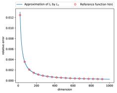
(a) Plots of $(L_{n}-l_{n})/L_{n}$ and $h(n)$.

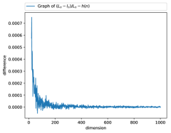
(b) Plot of $(L_{n}-l_{n})/L_{n}-h(n)$.

Figure 4:

6 Concluding remarks

Starting from the goal of learning an operational representation, we have studied a general class of generative latent variable models $x=f(z)$, where $f$ is a smooth stochastic process. The latent space can here be endowed with a random Riemannian metric, such that elementary operations (interpolations, distances, integration, etc.) can be defined in a way that is invariant to reparametrizations of the model.

Mathematically, this is a natural approach, but it does not lend itself easily to computations as computational tools do not exist for working with random Riemannian manifolds. In this paper we have provided a deterministic approximation to this large class of random Riemannian metrics, and provided tight approximation bounds. In particular, it is worth noting that the bound is very tight when data is high dimensional, which is the common case for machine learning. Within this deterministic approximation, we can apply standard tools for computations over Riemannian manifolds [18, 20, 13], and thereby realize the idea of operational representation learning.

References

- [1] R. J. Adler and J. E. Taylor. Random Fields and Geometry. Springer, 2007 edition, 2007.
- [2] G. Arvanitidis, L. K. Hansen, and S. Hauberg. Latent space oddity: on the curvature of deep generative models. International Conference on Learning Representations (ICLR), 2018.
- [3] R. G. Baraniuk and M. B. Wakin. Random projections of smooth manifolds. Foundations of Computational Mathematics, 9:51–77, 2009.
- [4] Mikhail Belkin and Partha Niyogi. Laplacian Eigenmaps for Dimensionality Reduction and Data Representation. Neural Computation, 15(6):1373–1396, June 2003.
- [5] G. Biau and D. M. Mason. High-dimensional p-norms. arXiv:1311.0587, 2013.
- [6] David M Blei, Alp Kucukelbir, and Jon D McAuliffe. Variational inference: A review for statisticians. Journal of the American Statistical Association, 112(518):859–877, 2017.
- [7] Avrim Blum. Random projection, margins, kernels, and feature-selection. In Craig Saunders, Marko Grobelnik, Steve Gunn, and John Shawe-Taylor, editors, Subspace, Latent Structure and Feature Selection, pages 52–68. Springer Berlin Heidelberg, 2006.
- [8] Kenneth L. Clarkson. Tighter bounds for random projections of manifolds. In Proceedings of the Twenty-fourth Annual Symposium on Computational Geometry, SCG ’08, pages 39–48, New York, NY, USA, 2008. ACM.
- [9] H. Cramér. Mathematical methods of statistics. Asia Publishing House, 1962.
- [10] Sanjoy Dasgupta and Anupam Gupta. An elementary proof of a theorem of Johnson and Lindenstrauss. Random Structures & Algorithms, 22(1):60–65, 2003.
- [11] David L. Donoho and Carrie Grimes. Hessian eigenmaps: Locally linear embedding techniques for high-dimensional data. Proceedings of the National Academy of Sciences, 100(10):5591–5596, 2003.
- [12] Carl-Gustav Esseen. On the remainder term in the central limit theorem. Ark. Mat., 8(1):7–15, 11 1969.
- [13] Oren Freifeld, Søren Hauberg, and Michael J. Black. Model transport: Towards scalable transfer learning on manifolds. In Proceedings IEEE Conf. on Computer Vision and Pattern Recognition (CVPR), Columbus, Ohio, USA, June 2014.
- [14] Yoav Freund, Sanjoy Dasgupta, Kabra Mayank, and Nakul Verma. Learning the structure of manifolds using random projections. In J. C. Platt, D. Koller, Y. Singer, and S. T. Roweis, editors, Advances in Neural Information Processing Systems 20, pages 473–480. Curran Associates, Inc., 2008.
- [15] Sylvestre Gallot, Dominique Hulin, and Jacques Lafontaine. Riemannian geometry, volume 3. Springer, 1990.
- [16] GPy. GPy: A Gaussian process framework in python. http://github.com/SheffieldML/GPy, 2012.
- [17] S. Hauberg. Only bayes should learn a manifold (on the estimation of differential geometric structure from data). arXiv:1806.04994, 2018.
- [18] Søren Hauberg, Oren Freifeld, and Michael J. Black. A geometric take on metric learning. In P. Bartlett, F.C.N. Pereira, C.J.C. Burges, L. Bottou, and K.Q. Weinberger, editors, Advances in Neural Information Processing Systems (NIPS) 25, pages 2033–2041. MIT Press, 2012.
- [19] Chinmay Hegde, Michael Wakin, and Richard Baraniuk. Random projections for manifold learning. In J. C. Platt, D. Koller, Y. Singer, and S. T. Roweis, editors, Advances in Neural Information Processing Systems 20, pages 641–648. Curran Associates, Inc., 2008.
- [20] Philipp Hennig and Søren Hauberg. Probabilistic solutions to differential equations and their application to Riemannian statistics. In Proceedings of the 17th international Conference on Artificial Intelligence and Statistics (AISTATS), volume 33, 2014.
- [21] R. A. Khan. Approximation for the expectation of a function of the sample mean. Statistics, 38:117–122, 2004.
- [22] Diederik P Kingma and Max Welling. Auto-Encoding Variational Bayes. In Proceedings of the 2nd International Conference on Learning Representations (ICLR), 2014.
- [23] Subhaneil Lahiri, Peiran Gao, and Surya Ganguli. Random projections of random manifolds. arXiv:1607.04331, 07 2016.
- [24] Neil Lawrence. Probabilistic non-linear principal component analysis with Gaussian process latent variable models. J. Mach. Learn. Res., 6:1783–1816, December 2005.
- [25] R. J. Muirhead. Aspects of Multivariate Statistical Theory. Wiley, 2005.
- [26] Xavier Pennec. Intrinsic Statistics on Riemannian Manifolds: Basic Tools for Geometric Measurements. Journal of Mathematical Imaging and Vision, 25(1):127–154, July 2006.
- [27] C. E. Rasmussen and C. K. I. Williams. Gaussian Processes for Machine Learning. The MIT Press, 2006.
- [28] Danilo Jimenez Rezende, Shakir Mohamed, and Daan Wierstra. Stochastic backpropagation and approximate inference in deep generative models. In Eric P. Xing and Tony Jebara, editors, Proceedings of the 31st International Conference on Machine Learning, volume 32 of Proceedings of Machine Learning Research, pages 1278–1286. PMLR, 2014.
- [29] Sam T Roweis and Lawrence K Saul. Nonlinear dimensionality reduction by locally linear embedding. Science, 290(5500):2323–2326, 2000.
- [30] Bernhard Schölkopf, Alexander Smola, and Klaus-Robert Müller. Kernel principal component analysis. In Advances in Kernel Methods - Support Vector Learning, pages 327–352, 1999.
- [31] Joshua B Tenenbaum, Vin De Silva, and John C Langford. A global geometric framework for nonlinear dimensionality reduction. Science, 290(5500):2319–2323, 2000.
- [32] Alessandra Tosi, Søren Hauberg, Alfredo Vellido, and Neil D. Lawrence. Metrics for probabilistic geometries. In The Conference on Uncertainty in Artificial Intelligence (UAI), Quebec, Canada, July 2014.
- [33] N. Verma. A note on random projections for preserving paths on a manifold. UC San Diego, Tech. Report CS2011-0971, 2011.