Analytical results for the distribution of shortest path lengths in directed random networks that grow by node duplication

Abstract

We present exact analytical results for the distribution of shortest path lengths (DSPL) in a directed network model that grows by node duplication. Such models are useful in the study of the structure and growth dynamics of gene regulatory networks and scientific citation networks. Starting from an initial seed network, at each time step a random node, referred to as a mother node, is selected for duplication. Its daughter node is added to the network and duplicates each outgoing link of the mother node with probability $p$. In addition, the daughter node forms a directed link to the mother node itself. Thus, the model is referred to as the corded directed-node-duplication (DND) model. In this network not all pairs of nodes are connected by directed paths, in spite of the fact that the corresponding undirected network consists of a single connected component. More specifically, in the large network limit only a diminishing fraction of pairs of nodes are connected by directed paths. To calculate the DSPL between those pairs of nodes that are connected by directed paths we derive a master equation for the time evolution of the probability $P_{t}(L=\ell)$, $\ell=1,2,\dots$, where $\ell$ is the length of the shortest directed path. Solving the master equation, we obtain a closed form expression for $P_{t}(L=\ell)$. It is found that the DSPL at time $t$ consists of a convolution of the initial DSPL $P_{0}(L=\ell)$, with a Poisson distribution and a sum of Poisson distributions. The mean distance ${\mathbb{E}}_{t}[L|L<\infty]$ between pairs of nodes which are connected by directed paths is found to depend logarithmically on the network size $N_{t}$. However, since in the large network limit the fraction of pairs of nodes that are connected by directed paths is diminishingly small, the corded DND network is not a small-world network, unlike the corresponding undirected network.

1 Introduction

The increasing interest in the field of complex networks in recent years is motivated by the realization that a large variety of systems and processes in physics, chemistry, biology, engineering, and society can be usefully described by network models Albert2002 ; Caldarelli2007 ; Havlin2010 ; Newman2010 ; Estrada2011b ; Barrat2012 . These models consist of nodes and edges, where the nodes represent physical objects, while the edges represent the interactions between them. A common feature of complex networks is the small-world property, namely the fact that the mean distance and the diameter scale like $\ln N$, where $N$ is the network size Milgram1967 ; Watts1998 ; Chung2002 ; Chung2003 . Many of these networks are scale-free, which means that they exhibit power-law degree distributions Barabasi1999 ; Jeong2000 ; Krapivsky2000 ; Krapivsky2001 ; Vazquez2003 . The most highly connected nodes, called hubs, play a dominant role in dynamical processes on these networks. Moreover, it was shown that scale-free networks are generically ultrasmall, namely their mean distance and diameter scale like $\ln\ln N$ Cohen2003 .

While pairs of adjacent nodes exhibit direct interactions, the interactions between most pairs of nodes are indirect, and are mediated by intermediate nodes and edges. Pairs of nodes may be connected by many different paths. The shortest among these paths are of particular importance because they are likely to provide the fastest and strongest interactions. Therefore, it is of much interest to study the distribution of shortest path lengths (DSPL) between pairs of nodes in different types of networks. The DSPL is of great importance for the temporal evolution of dynamical processes Barrat2012 , such as signal propagation in genetic regulatory networks Giot2003 ; Maayan2005 , navigation Dijkstra1959 ; Delling2009 and epidemic spreading Satorras2015 . Central measures of the DSPL such as the mean distance and extremal measures such as the diameter were studied Watts1998 ; Bollobas2001 ; Durrett2007 ; Fronczak2004 ; Newman2001b ; Hartmann2017 . However, apart from a few studies Newman2001 ; Dorogotsev2003 ; Blondel2007 ; Hofstad2007 ; Esker2008 ; Shao2008 ; Shao2009 , the DSPL has not attracted nearly as much attention as the degree distribution. Recently, an analytical approach was developed for calculating the DSPL Katzav2015 in the Erdős-Rényi (ER) network Erdos1959 ; Erdos1960 ; Erdos1961 , which is the simplest mathematical model of a random network. More general formulations were later developed Nitzan2016 ; Melnik2016 , for the broader class of configuration model networks Newman2001 ; Molloy1995 ; Molloy1998 .

To gain insight into the structure of complex networks, it is useful to study the growth dynamics that gives rise to these structures. In general, it appears that many of the networks encountered in biological, ecological and social systems grow step by step, by the addition of new nodes and their attachment to existing nodes. A common feature of these growth processes is the preferential attachment mechanism, in which the likelihood of an existing node to gain a link to the new node is proportional to its degree. It was shown that growth models based on preferential attachment give rise to scale-free networks, which exhibit power-law degree distributions Albert2002 ; Barabasi1999 . The effect of node duplication (ND) processes on network structure was studied using an undirected network growth model in which at each time step a random node, referred to as a mother node, is selected for duplication and its daughter node duplicates each link of the mother node with probability $p$ Bhan2002 ; Kim2002 ; Chung2003b ; Krapivsky2005 ; Ispolatov2005 ; Ispolatov2005b ; Bebek2006 ; Li2013 . In this model the daughter node does not form a link to the mother node, and thus in the following it is referred to as the uncorded ND model. It was shown that for $0<p<1/2$ the resulting network exhibits a power law degree distribution of the form

$$P(K=k)\sim k^{-\gamma}.$$ (1)

For $0<p<1/e$, where $e$ is the base of the natural logarithm, the exponent is given by the nontrivial solution of the equation $\gamma=3-p^{\gamma-2}$, while for $1/e\leq p<1/2$ it takes the value $\gamma=2$ Ispolatov2005 . For $1/2\leq p\leq 1$ the degree distribution does not converge to an asymptotic form.

Recently, a different variant of an undirected node duplication model was introduced and studied Lambiotte2016 ; Bhat2016 . In this model, referred to as the corded ND model, at each time step a random mother node, M, is selected for duplication. The daughter node, D, is added to the network. It forms an undirected link to its mother node, M, and is also connected with probability $p$ to each neighbor of M. It was shown that for $0<p<1/2$ the corded ND model generates a sparse network, while for $1/2\leq p\leq 1$ the model gives rise to a dense network in which the mean degree increases with the network size Lambiotte2016 ; Bhat2016 . For $0<p<1/2$ the degree distribution of this network follows a power-law distribution, given by Eq. (1), where the exponent $\gamma$ is given by the non-trivial solution of the equation $\gamma=1+p^{-1}-p^{\gamma-2}$ Lambiotte2016 ; Bhat2016 . In the limit of $p\rightarrow 0$, the exponent diverges like $\gamma\sim 1/p$. This model is suitable for the description of acquaintance networks, in which a newcomer who has a friend in the community becomes acquainted with other members Toivonen2009 . Unlike the uncorded ND model, the formation of triadic closures is built-in to the dynamics of the corded ND model. This means that once the daughter node forms a link to a neighbor of the mother node, it completes a triangle in which the mother, neighbor and daughter nodes are all connected to each other. The formation of triadic closures is an essential property of the dynamics of social networks Granovetter1973 . The formation of triadic closures is in sharp contrast to configuration model networks, which exhibit a local tree-like structure. Interestingly, many empirical networks exhibit a high abundance of triangles, both in undirected networks Newman2001b and in directed networks, where most triangles form feed-forward loops (FFLs), while triangular feedback loops are rare Milo2002 ; Alon2006 . Unlike configuration model networks Newman2001 ; Molloy1995 ; Molloy1998 , which may include small, isolated components, the corded ND network consists of a single connected component. Therefore, it does not exhibit a percolation transition.

In a recent paper, we studied the DSPL of the (undirected) corded ND network Steinbock2017 . Focusing on the sparse network regime of $0<p<1/2$, we derived a master equation for the time evolution of the probabilities $P_{t}(L=\ell)$, where $\ell=1,2,\dots$ is the distance between a pair of nodes and $t$ is the time. Solving the master equation we obtained an expression for $P_{t}(L=\ell)$, which consists of two convolution-like sums. The first sum emanates from the DSPL of the seed network $P_{0}(L=\ell)$, while the second sum involves a discrete exponential function. We calculated the mean distance $\langle L\rangle_{t}$, and the diameter, $\Delta_{t}$, and showed that in the long-time limit they scale like $\ln t$, namely the corded ND network is a small-world network Milgram1967 ; Watts1998 ; Chung2002 ; Chung2003 .

In a more recent paper we introduced a directed version of the corded node duplication network model and studied its in-degree and out-degree distributions Steinbock2018 . This model is referred to as the corded directed node duplication (DND) model. At each time step a random mother node is chosen for duplication. The daughter node forms a directed link to the mother node and with probability $p$ to each outgoing neighbor of the mother node. This model may be useful in the study of gene regulatory networks. These are directed networks that evolve by gene duplication Ohno1970 ; Teichmann2004 . It also describes the structure and dynamics of scientific citation networks Redner1998 ; Redner2005 ; Radicchi2008 ; Golosovsky2012 ; Golosovsky2017a ; Golosovsky2017b , in which the nodes represent papers, while the links represent citations. Scientific citation networks are directed networks, with links pointing from the later (citing) paper to the earlier (cited) paper. A paper A, citing an earlier paper B, often also cites one or several papers C, which were cited in B Peterson2010 . The resulting network module is a triangle, or triadic closure, which includes three directed links, from A to B, from B to C and from A to C and thus resembles the FFL structure. However, the links of this module point backwards, and thus it may be more suitable to refer to it as a feed-backward loop (FBL). The functionality of FBLs is different from that of FFLs. FFLs typically appear in information processing networks, enabling the interference between signals propagating along two different paths. In contrast, FBLs track the source of the cited information both directly and indirectly via an intermediate reference point. Due to the directionality of the links, each node exhibits both an in-degree, which is the number of incoming links and an out-degree which is the number of outgoing links. Therefore, the degree distribution consists of two separate distributions, namely the distribution $P_{t}(K_{\rm in}=k)$ of in-degrees and the distribution $P_{t}(K_{\rm out}=k)$ of out-degrees, at time $t$. These two distributions are related to each other by the constraint that their means must be equal, namely $\langle K_{\rm in}\rangle_{t}=\langle K_{\rm out}\rangle_{t}$. We obtained exact analytical results for the in-degree distribution and the out-degree distribution of the corded DND network Steinbock2018 . It was found that the in-degrees follow a shifted power-law distribution while the out-degrees follow a narrow distribution that converges to a Poisson distribution in the sparse network limit and to a Gaussian distribution in the dense network limit. Since the network is directed not all pairs of nodes are connected by directed paths even though the corresponding undirected network consists of a single connected component. We also obtained analytical results for the distribution of the number of upstream nodes $P_{t}(N_{\rm up}=n)$, and for the distribution of the number of downstream nodes $P_{t}(N_{\rm down}=n)$, and show that $\langle N_{\rm up}\rangle=\langle N_{\rm down}\rangle$ are logarithmic in the network size. This means that in the large network limit only a diminishing fraction of pairs of nodes are connected by directed paths.

In this paper we present exact analytical results for the DSPL of the corded DND network. In order to calculate the DSPL we derive a master equation for the time evolution of the probability $P_{t}(L=\ell)$ that the shortest directed path from a random node $i$ to a random node $j$ at time $t$ is of length $\ell$, where the probability that there is no directed path from $i$ to $j$ is given by $P_{t}(L=\infty)$. Solving the master equation we obtain a closed form analytical expression for the DSPL, which consists of two terms. The first term is a convolution of the initial DSPL $P_{0}(L=\ell)$, with a Poisson distribution, while the second term is a sum of Poisson distributions. The mean distance ${\mathbb{E}}_{t}[L|L<\infty]$, between pairs of nodes that are connected by directed paths, is found to be logarithmic in the network size $N_{t}$. However, in the large network limit the fraction of pairs of nodes that are connected by directed paths is diminishingly small. Therefore, the corded DND network is not a small-world network, unlike the corresponding undirected network.

The paper is organized as follows. In Sec. 2 we present the corded DND model. In Sec. 3 we consider the distribution of degeneracy levels, $P(G=g)$, of the shortest paths between random pairs of nodes. In Sec. 4 we analyze the effect of these degeneracies on the DSPL. In Sec. 5 we provide a closed form analytical expression for $P_{t}(L=\ell)$, using a slightly approximated version of the master equation. The mean distance is calculated in Sec. 6 and the variance of the DSPL is evaluated in Sec. 7. The results are discussed in Sec. 8 and summarized in Sec. 9. In Appendix A we consider the set of canonical downstream configurations, which is used in the analysis of the degeneracies of shortest paths. In Appendix B we present the master equation for the temporal evolution of the degeneracy distribution $P_{t}(G=g)$, truncated at $g=2$ and evaluate the rate of congergence to the asymptotic form. In Appendix C we present the exact form of the master equation for the DSPL, and its time dependent solution, without the approximation used in Sec. 5.

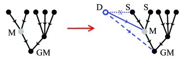
Figure 1: Illustration of the corded DND model. A random node, referred to as a mother node, M (gray circle) is selected for duplication. The newly formed daughter node, D (empty circle) deterministically acquires a directed link (solid line) to the mother node. It also acquires, with probability $p$, a directed link (dashed line) to each one of the outgoing neighbors of M. In this example, D forms a directed link to its grandmother node, denoted by GM. The model does not allow D to form links to its sister nodes, denoted by S, because they are incoming neighbors rather than outgoing neighbors of M.

2 The corded directed node duplication model

In the corded DND model, at each time step during the growth phase of the network, a random node, referred to as a mother node, is selected for duplication. The daughter node is added to the network, forming a directed link to the mother node. Also, with probability $p$, it forms a directed link to each outgoing neighbor of the mother node (Fig. 1). The growth process starts from an initial seed network of $N_{0}=s$ nodes. Thus, the network size after $t$ time steps is $N_{t}=t+s$. In Fig. 2 we present two instances of the corded DND network, of size $N_{t}=50$, which were formed around the same backbone tree. Both networks were grown from a seed network of size $s=2$, with $p=0.2$ [Fig. 2(a)] and $p=0.5$ [Fig. 2(b)]. Thus, each network instance includes $N_{t}-1=49$ deterministic links (solid lines). The network of Fig. 2(b) is denser and includes $39$ probabilistic links (dashed lines), compared to $19$ probabilistic links in Fig. 2(a).

Upon formation, the in-degree of the daughter node is zero. The incoming links are gradually formed as the daughter node matures. Since the mother node at time $t$ is selected randomly from all the $N_{t}$ nodes in the network, its in-degree is effectively drawn from the in-degree distribution $P_{t}(K_{\rm in}=k)$. The mother node gains an incoming link from the daughter node, thus its in-degree increases by $1$. The daughter node gains one outgoing link to the mother node, and with probability $p$ it duplicates outgoing links of the mother node. Thus, in the case that all the outgoing links of the mother node are duplicated, the out-degree of the daughter node becomes $k_{\rm out}^{\rm D}=k_{\rm out}^{\rm M}+1$. In the case that none of the outgoing links of the mother node are duplicated the out-degree of the daughter node becomes $k_{\rm out}^{\rm D}=1$.

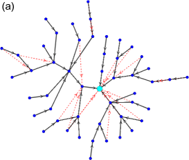
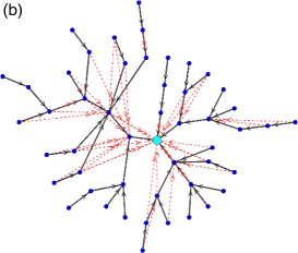
Figure 2: Two instances of corded DND networks of size $N=50$, with $p=0.2$ (a) and $p=0.5$ (b). Both networks were grown from a seed network that consists of two nodes connected by a directed link. For the sake of comparison, both instances are formed around the same backbone tree (solid lines). The sink node, which can be reached from all the other nodes in the network via directed paths is shown by a large circle. The probabilistic links (dashed lines) essentially decorate the tree. Increasing $p$ makes the network denser.

In order to obtain a network that consists of a single connected component, it is required that the seed network consist of a single connected component. The size of the seed network is denoted by $s$. Since the corded DND model generates oriented networks with no bidirectional edges, we restrict the analysis to seed networks in which a pair of nodes cannot be connected in both directions. Moreover, we consider only acyclic seed networks, namely networks that do not include any directed cycles. Finally, we focus on seed networks that include a single sink node, namely a node that has only incoming links and no outgoing links. The sink node can be reached via directed paths from all the nodes in the seed network. The in-degree distribution of the seed network is denoted by $P_{0}(K_{\rm in}=k)$ and its out-degree distribution is denoted by $P_{0}(K_{\rm out}=k)$. Clearly, the mean of the in-degree distribution and the mean of the out-degree distribution are equal to each other. We thus denote $\langle K\rangle_{0}=\langle K_{\rm in}\rangle_{0}=\langle K_{\rm out}\rangle_{0}$.

The DSPL of the seed network is denoted by $P_{0}(L=\ell)$, $\ell=1,2,\dots,s-1$. The probability that a random pair of nodes $i$ and $j$, in the seed network, are connected by a directed path from $i$ to $j$ is denoted by

$$P_{0}(L<\infty)=\sum_{\ell=1}^{s-1}P_{0}(L=\ell).$$ (2)

The complementary probability, $P_{0}(L=\infty)=1-P_{0}(L<\infty)$, is the probability that there is no directed path from $i$ to $j$. The mean distance between directed pairs of nodes in the seed network that are connected by directed paths is denoted by

$$\langle L\rangle_{0}=\frac{\sum\limits_{\ell=1}^{s-1}\ell P_{0}(L=\ell)}{P_{0}(L<\infty)}.$$ (3)

The DSPL and the mean in-degree (or out-degree) of the seed network are related by $P_{0}(L=1)=\langle K\rangle_{0}/(s-1)$. The probability $P_{0}(L=\ell)$ may take non-zero values for $\ell=1,2,\dots,\Delta_{0}$, where $\Delta_{0}$ is the diameter of the seed network, while $P_{0}(L=\ell)=0$ for $\ell\geq\Delta_{0}+1$. For seed networks of $s$ nodes, $\Delta_{0}$ may take values in the range $1\leq\Delta_{0}\leq s-1$.

To avoid memory effects, which may slow down the convergence to the asymptotic structure, it is often convenient to use a seed network that consists of a single node, namely $s=1$. For a seed network that consists of a single node the initial DSPL at $t=0$ is not defined. However, the DSPL becomes well defined at time $t=1$, when the network consists of a pair of connected nodes, whose DSPL is given by $P_{1}(L=\ell)=\delta_{\ell,1}/2$, where $\delta_{\ell,\ell^{\prime}}$ is the Kronecker delta, and $P_{1}(L=\infty)=1/2$, while its diameter is $\Delta_{1}=1$. Another interesting choice for the seed network is a linear chain of $s$ nodes, in which all the links are in the same direction. In this case, the initial DSPL is

$$P_{0}(L=\ell)=\frac{s-\ell}{s(s-1)},$$ (4)

for $\ell=1,2,\dots,s-1$ and $P_{0}(L=\infty)=1/2$. This choice captures the largest possible diameter in a seed network of $s$ nodes, namely $\Delta_{0}=s-1$. For simplicity, all the analytical results and the corresponding simulation results presented in the Figures below, were obtained for a seed network that consists of a linear chain with $s=2$, namely a pair of nodes with a single directed link between them.

The mother-daughter links in the corded DND network form a random directed tree structure, which serves as a backbone tree for the resulting network. The backbone tree is a random directed recursive tree Smythe1995 ; Drmota1997 ; Drmota2005 . To study its properties, one can take the limit of $p=0$, in which the corded DND network is reduced to the backbone tree.

3 The degeneracy of the shortest paths

Consider a pair of nodes $i$ and $j$ for which there is at least one directed path from $i$ to $j$. In the case that the shortest path from $i$ to $j$ is of length $\ell\geq 2$, this path may be unique or it may be degenerate. In the case that the shortest path is degenerate, there are at least two different paths of length $\ell$ from $i$ to $j$ (which may have overlapping segments). In particular, the degenerate paths may differ in the first step, starting from node $i$. Here we focus on the degeneracy of the first step, namely on the number of outgoing neighbors of $i$ which reside on shortest paths from $i$ to $j$. The number of such distinct neighbors is denoted by $g$. We denote the distribution of the degeneracy levels of the first steps of the shortest paths by $P(G=g)$, where $g=1,2,\dots$. In order to calculate the distribution $P(G=g)$ we follow the growth process of the network and consider the shortest path from the newly formed daughter node, D, to a randomly selected node T downstream of M. It is important to note that the distances $\ell_{\rm DT}$ between the daughter node, D, and all the accessible nodes, T, downstream of M are determined upon formation of the node D. This is due to the fact that nodes and edges which will be added later cannot form paths between D and T which are shorter than $\ell_{\rm DT}$. Moreover, unlike the case of the corded undirected ND model, they cannot even form additional paths of length $\ell_{\rm DT}$ between D and T. This means that the degeneracies of the shortest paths from D to all downstream nodes are also determined upon formation of D.

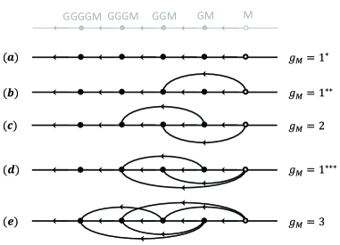
Figure 3: Illustration of possible network structures in the vicinity of a newly formed daughter node D and its mother node M. The grandmother (GM) node, the great-grandmother (GGM) node and two more generations are also marked downstream of M. The deterministic links are represented by straight horizontal arrows while the probabilistic links are represented by arcs. (a) A linear branch of the backbone tree (marked by $g_{\rm M}=1^{*}$), consisting of a succession of mother-daughter pairs connected by deterministic links and no probabilistic links. The nodes which are accessible from M reside downstream, on the left hand side. The degeneracy of the first step in the paths from M to all the nodes that are accessible from M along directed paths is $g=1$; (b) A configuration in which M forms a probabilistic path to GGM (marked by $g_{\rm M}=1^{**}$). The degeneracies of the downsteam paths from M are $g=1$. However, this configuration differs from the configuration shown in (a) in the sense that in a future step, when M will be selected for duplication, its daughter node D may acquire degeneracy $g=2$ by forming a probabilistic link to GM; (c) A configuration in which the degeneracy of the first step in the paths from M to GGGM and all downstream nodes is $g=2$ (marked by $g_{\rm M}=2$). (d) In this configuration (marked by $g_{\rm M}=1^{***}$), the degeneracy of the paths downstream of M is $g=1$. However, upon future duplication of M, its daughter node D may acquire a degeneracy of $g=3$ for their paths to GGGM and all downstream nodes, by forming probabilistic links to GM and GGM. (e) A configuration in which the degeneracy of the first step in the paths from M to GGGM and all its downstream nodes is $g=3$ (marked by $g_{\rm M}=3$).

In order to analyze the distribution of degeneracies, $P(G=g)$ we will first classify all the possible local configurations downstream of a random node $i$. These configurations determine the degeneracy of the paths from $i$ to all its downstream nodes. In Fig. 3 we present an illustration of the possible network structures in the downstream vicinity of a random node upon its selection as a mother node, M. The grandmother (GM) node and the great-grandmother (GGM) node, as well as two earlier generations (GGGM and GGGGM) are also marked downstream of M. The deterministic links are represented by straight horizontal arrows, pointing to the left. The probabilistic links are represented by arcs. More specifically, in Fig. 3(a) we present a linear branch of the backbone tree (marked by $g_{\rm M}=1^{*}$), consisting of a succession of mother-daughter pairs connected by deterministic links and no probabilistic links. The nodes which are accessible from M reside downstream, on the left hand side. The degeneracy of the first step in the paths from M to all the nodes which are accessible from M along directed paths is $g=1$; In Fig. 3(b) we present a configuration in which M forms a probabilistic path to GGM. The degeneracies of the directed paths from M to downsteam nodes is $g=1$. However, in this configuration (marked by $g_{\rm M}=1^{**}$), upon duplication of M, its daughter node, D, may acquire degeneracy $g=2$ by forming a probabilistic link to GM. In Fig. 3(c) we present a configuration in which the degeneracy of the first step in the paths from M to GGGM and all downstream nodes is $g=2$ (marked by $g_{\rm M}=2$). This is due to the fact that there are two different paths of length $\ell=2$ from M to GGGM, one path via GM and the other via GGM. In Fig. 3(d) we present a configuration (marked by $g_{\rm M}=1^{***}$), in which the degeneracy of the shortest paths to all the nodes that reside downstream of M is $g=1$. However, upon duplication of M, its daughter node D may acquire degeneracy of $g=3$ for the path to GGGM and all downstream nodes. In order to acquire such degeneracy, D should duplicate the links from M to GM and to GGM, but should not duplicate the link to GGGM. In general, the notation $g_{\rm M}=1^{**\dots*}$ represents configurations in which the degeneracy of the paths downstream of the mother node is $g=1$, while the number of stars represents the highest possible degeneracy of the paths downstream of the daughter node. In Fig. 3(e) we present a configuration in which the degeneracy of the shortest paths from M to GGGGM and all its downstream nodes is $g=3$ (marked by $g_{\rm M}=3$). This is due to the fact that there are three degenerate shortest paths of length $\ell=2$ from M to GGGGM: a path via GM, another path via GGM and a third path via GGGM.

In Fig. 4 we present the evolution of the local downstream configuration and the degeneracies of shortest paths, from a mother node M to its daughter node D, upon duplication of M. In the top line we show a random node, denoted by M, upon its selection for duplication. The deterministic link from the daughter node D to M is presented by a dashed line. The node D may form probabilistic links to the two outgoing neighbors of M, namely GM and GGM. Each one of the two links is formed with probability $p$, and thus there are four possible downstream configurations for D. In Fig 4(a) we present the case in which no probabilistic links were formed. The resulting degeneracy of the paths from D to all the downstream nodes is $g=1$. Therefore, with respect to the shortest paths and their degeneracies, this configuration is equivalent to $g_{\rm D}=1^{*}$ (Appendix A). In Fig. 4(b) we present the case in which the link to GM was duplicated, but the link to GGM was not duplicated. In this case the degeneracies of the shortest paths from D to GGM and all its downstream nodes is $g=2$ ($g_{D}=2$). In Fig. 4(c) we present the case in which the probabilistic links to both GM and GGM are formed. The resulting configuration is $g_{\rm D}=1^{***}$, in which the degeneracies of the shortest paths from D to all its downstream nodes are $g=1$, but its future offsprings may acquire a double or triple degeneracy. In Fig. 4(d) we show the case in which the link to GGM is duplicated, while the link to GM is not duplicated. In this case the degeneracies of the shortest paths from D to its downstream nodes is $g=1$ This configuration is equivalent to $g_{D}=1^{**}$ (Appendix A).

Figure 4: The evolution of the local downstream configuration and the degeneracies of shortest paths, from a mother node, M, to its daughter node D upon duplication of M. Top line: a random node, denoted by M, is selected for duplication. The deterministic link from the daughter node D to M is shown (dashed line). The node D may form probabilistic links to the two outgoing neighbors of M, referred to as GM and GGM. Each one of the two links is formed with probability $p$, and thus there are four possible downstream configurations for D. (a) None of the links are formed and the resulting degeneracy is $g=1$ (Configuration $g_{\rm D}=1^{*}$); (b) Only the link from D to GM is formed, giving rise to $g=2$ (Configuration $g_{\rm D}=2$); (c) Both links are formed and the resulting degeneracy is $g=1$ (configuration $g_{\rm D}=1^{***}$); (d) Only the link to GGM is formed and the resulting degeneracy is $g=1$ (configuration $g_{\rm D}=1^{**}$).

The probability distribution of the degeneracies of a randomly selected mother node, M, at time $t$, is given a vector of the form $\vec{P}_{t}^{\rm M}(G=g)$. The elements of this vector represent the probabilities of the downstream configurations of M, given by $g=1^{*},1^{**},2,1^{***},3,\dots,g_{\rm max}$, where $g_{\rm max}$ is the truncation degeneracy level. The transition probability from a configuration $g_{\rm M}$, of the mother node, to a configuration $g_{\rm D}$ of its daughter node, is denoted by $P(g_{\rm M}\rightarrow g_{\rm D})$. We present these transition probabilities in a matrix $T$, such that

$$\vec{P}_{t}^{\rm D}(G=g)=T\vec{P}_{t}^{\rm M}(G=g).$$ (5)

To demonstrate the dynamical evolution of the degeneracy we first consider a truncated set of equations, which includes only three configurations: $g=1^{*}$, $g=1^{**}$ and $g=2$. In this case, the probability distribution of the degeneracies of a randomly selected mother node M, at time $t$, is given by the vector

$$\vec{P}_{t}^{\rm M}(G=g)=\left[\begin{array}[]{l}P_{t}^{\rm M}(G=1^{*})\\ P_{t}^{\rm M}(G=1^{**})\\ P_{t}^{\rm M}(G=2)\end{array}\right].$$ (6)

The probability distribution of the daughter node is given by the corresponding vector $\vec{P}_{t}^{\rm D}(G=g)$. The $3\times 3$ transition matrix takes the form

$$T=\left[\begin{array}[]{ccc}1-p&(1-p)^{2}&(1-p)^{2}\\ p&p&2p(1-p)\\ 0&p(1-p)&p^{2}\end{array}\right].$$ (7)

Note that this matrix satisfies the condition $\sum_{i=1}^{3}T_{i,j}=1$ for $j=1$, $2$ and $3$, so probability is conserved. In order to truncate the equations, we use a closure condition in which the transition probability $T_{4,2}=P(1^{**}\rightarrow 1^{***})=p^{2}$ is added to $T_{2,2}=P(1^{**}\rightarrow 1^{**})$. Solving for the steady state of the equation $\vec{P}(G=g)=T\vec{P}(G=g)$, under the condition that $P(G=1^{*})+P(G=1^{**})+P(G=2)=1$, we obtain

$$P(G=1^{*}) = \frac{(1-p)^{2}}{1-p+p^{2}}$$

$$P(G=1^{**}) = \frac{p(1+p)}{(1+2p)(1-p+p^{2})}$$

$$P(G=2) = \frac{p^{2}}{(1+2p)(1-p+p^{2})}.$$ (8)

Summing up the contributions to $g=1$, using $P(G=1)=P(G=1^{*})+P(G=1^{**})$, we obtain

$$P(G=1) = \frac{1+p-2p^{2}+2p^{3}}{(1+2p)(1-p+p^{2})}$$

$$P(G=2) = \frac{p^{2}}{(1+2p)(1-p+p^{2})}.$$ (9)

Extending the analysis up to degeneracy $g=3$, the probability distribution of the degeneracies of all the nodes in the network at time $t$ is described by the vector

$$\vec{P}_{t}(G=g)=\left[\begin{array}[]{l}P_{t}(G=1^{*})\\ P_{t}(G=1^{**})\\ P_{t}(G=2)\\ P_{t}(G=1^{***})\\ P_{t}(G=3)\end{array}\right],$$ (10)

and the transition matrix takes the form

$$T=$$

$$\left[\begin{array}[]{ccccc}1-p&(1-p)^{2}&(1-p)^{2}&(1-p)^{3}&(1-p)^{3}\\ p&p(1-p)&2p(1-p)&p(1-p)^{2}&3p(1-p)^{2}\\ 0&p(1-p)&p^{2}&2p(1-p)^{2}&3p^{2}(1-p)\\ 0&p^{2}&0&p^{2}(2-p)&0\\ 0&0&0&p^{2}(1-p)&p^{3}\end{array}\right].$$ (16)

(17)

Solving for the asymptotic steady state solution of the degeneracy vector, given by $\vec{P}(G=g)=T\vec{P}(G=g)$, we obtain

$$P(G=1^{*})=\frac{(1-p)^{2}(1+3p+2p^{2}-2p^{4}-2p^{5}+p^{6})}{1+2p+p^{3}+p^{4}+2p^{5}+4p^{6}-p^{7}+p^{8}}$$

$$P(G=1^{**})=\frac{p(1+2p-2p^{3}-2p^{4}+p^{6})}{1+2p+p^{3}+p^{4}+2p^{5}+4p^{6}-p^{7}+p^{8}}$$

$$P(G=2)=\frac{p^{2}(1+p+p^{2}-p^{3}-p^{4}+2p^{5})}{1+2p+p^{3}+p^{4}+2p^{5}+4p^{6}-p^{7}+p^{8}}$$

$$P(G=1^{***})=\frac{p^{3}(1+2p+2p^{2}+p^{3})}{1+2p+p^{3}+p^{4}+2p^{5}+4p^{6}-p^{7}+p^{8}}$$

$$P(G=3)=\frac{p^{5}(1+p)}{1+2p+p^{3}+p^{4}+2p^{5}+4p^{6}-p^{7}+p^{8}}.$$

(18)

Summing up the three components which correspond to single degeneracy, we obtain the probability $P(G=1)=P(G=1^{*})+P(G=1^{**})+P(G=1^{***})$. The distribution of degeneracy levels at steady state is thus given by

$$P(G=1)=\frac{1+2p-p^{2}+2p^{5}+4p^{6}-3p^{7}+p^{8}}{1+2p+p^{3}+p^{4}+2p^{5}+4p^{6}-p^{7}+p^{8}}$$

$$P(G=2)=\frac{p^{2}(1+p+p^{2}-p^{3}-p^{4}+2p^{5})}{1+2p+p^{3}+p^{4}+2p^{5}+4p^{6}-p^{7}+p^{8}}$$

$$P(G=3)=\frac{p^{5}(1+p)}{1+2p+p^{3}+p^{4}+2p^{5}+4p^{6}-p^{7}+p^{8}}.$$

(19)

One can easily confirm that the probabilities in Eq. (19) satisfy the normalization condition, namely $P(G=1)+P(G=2)+P(G=3)=1$. In the limit of $p\ll 1$ Eq. (19) can be approximated by

$$P(G=1) = 1-p^{2}(1-p)+O(p^{4})$$

$$P(G=2) = p^{2}(1-p)+O(p^{4})$$

$$P(G=3) = p^{5}(1-p)+O(p^{7}).$$ (20)

This reflects the fact that the double degeneracy requires two probabilistic links while the triple degeneracy requires five probabilistic links. In both cases in order to maintain the degeneracy, the probabilistic link that would shorten the degenerate paths and remove the degeneracy should not form. This occurs with probability $1-p$.

4 The effect of the degeneracy on the DSPL

A node which resides at distance $\ell$ downstream of the mother node, may end up either at distance $\ell$ or at distance $\ell+1$ from the daughter node. To exemplify this property, consider a target node T at distance $\ell$ from the mother node M. A shortest path from M to T consists of a set of nodes ${\rm M},r_{1},r_{2},\dots,r_{\ell-1},{\rm T}$ in which subsequent nodes are connected by directed links. In the case that the link between M and $r_{1}$ is duplicated by D, the node T ends up at a distance $\ell$ from D, while in the case it is not duplicated, the node T ends up at distance $\ell+1$ from D. In the case that there is a single shortest path from M to T, the former scenario would occur with probability $p$ while the latter scenario would occur with probability $1-p$, namely

$$P_{t}^{\rm D}(L=\ell)=pP_{t}^{\rm M}(L=\ell)+(1-p)P_{t}^{\rm M}(L=\ell-1),$$ (21)

where $\ell\geq 2$. However, since shortest paths of lengths $\ell\geq 2$ from M to T may be degenerate, the calculation of $P_{t}^{\rm D}(L=\ell)$ requires a more careful attention. For $\ell\geq 3$ we express the DSPL between the daughter node D and the nodes that reside downstream of M in the form

$$P_{t}^{\rm D}(L=\ell)=\eta P_{t}^{\rm M}(L=\ell)+(1-\eta)P_{t}^{\rm M}(L=\ell-1).$$ (22)

where $0<\eta<1$. The case of $\ell=2$ is special in the sense that it combines the parameters $p$ and $\eta$. It takes the form

$$P_{t}^{\rm D}(L=2)=\eta P_{t}^{\rm M}(L=2)+(1-p)P_{t}^{\rm M}(L=1).$$ (23)

Apart from the special treatment of paths of lengths $1$ and $2$, it is assumed that $\eta=\eta(p)$ does not depend on the path length $\ell$.

In order to evaluate the parameter $\eta$, consider a random target node T, which is at distance $\ell$ from the mother node M. Here we are concerned with the degeneracy of the first step along the shortest paths. This degeneracy is given by the number of nearest neighbors of M which reside on at least one shortest path from M to T, and is denoted by $g$. Clearly, $g\leq k$, where $k$ is the degree of the mother node, M. In the case that node M is chosen for duplication, if none of the $g$ links of M which reside on shortest paths to T are duplicated, the distance between the daughter node D and T becomes $\ell+1$, while in the case that at least one of these $g$ edges is duplicated, the distance is $\ell$. Since each link of the mother node M is duplicated with probability $p$, the probability that none of them is duplicated is $(1-p)^{g}$. The probability that at least one of these $g$ links will be duplicated is $1-(1-p)^{g}$. Thus, the probability $\eta$ that at least one of the $g$ neighbors of the mother node M, which reside along shortest paths to T, are connected to the daughter node can be expressed by

$$\eta=1-\sum_{g=1}^{\infty}(1-p)^{g}P(G=g).$$ (24)

Inserting $P(G=g)$ for $g=1$ and $2$ from Eq. (9) into Eq. (24), we obtain

$$\eta=p+\frac{p^{3}(1-p)}{1+p-p^{2}+2p^{3}}.$$ (25)

Inserting $P(G=g)$ for $g=1$, $2$ and $3$, from Eq. (19) into Eq. (24), we obtain

$$\eta=p+\frac{(1-p)p^{3}\left(1+p+p^{2}+p^{3}+p^{5}\right)}{1+2p+p^{3}+p^{4}+2p^{5}+4p^{6}-p^{7}+p^{8}}.$$ (26)

In Fig. 5 we present the parameter $\eta$ as a function of $p$. The analytical results obtained from Eq. (25), which takes into account only single and double degeneracies, are shown by a dashed line. The results obtained from Eq. (26), which takes into account single, double and triple degeneracies, are shown by a solid line. The difference between the two curves is very small, indicating that the results are well converged and that the effect of higher order degeneracies is negligible. For small values of $p$, where most of the shortest paths are non-degenerate, $\eta$ is essentially equal to $p$. As $p$ is increased, the shortest paths are more likely to be degenerate. As a result, the probability $\eta$ becomes larger than $p$. In the limit of $p\rightarrow 1$ the two probabilities converge. The analytical results are found to be in very good agreement with the results obtained from computer simulations (symbols) for network sizes of $N_{t}=10^{2}$ ($\times$), $10^{4}$ ($+$) and $10^{6}$ ($\circ$).

Figure 5: The probability $\eta$ that the shortest path length from the daughter node D to any downstream node T is equal to the shortest path length from its mother node M to T, as a function of $p$. The analytical results obtained from Eq. (25), which takes into account only single and double degeneracies, are shown by a dashed line, while the results obtained from Eq. (26), which takes into account single, double and triple degeneracies, are shown by a solid line. The difference between the two curves is very small, indicating that the results are well converged and that the effect of higher order degeneracies is negligible. For small values of $p$, where the shortest paths are non-degenerate, $\eta$ is essentially equal to $p$. As $p$ is increased, the shortest paths are more likely to be degenerate. As a result, the probability $\eta$ becomes larger than $p$. In the limit of $p\rightarrow 1$ the two probabilities converge. The analytical results are found to be in very good agreement with the results obtained from computer simulations (symbols) for network sizes of $N_{t}=10^{2}$, $10^{4}$ and $10^{6}$.

5 The distribution of shortest path lengths

Consider an instance of the corded DND network. At time $t$ there are $N_{t}(N_{t}-1)$ directed pairs of nodes, in the network. The probability that the shortest directed path from a random node, $i$, to another random node $j$ is of length $\ell$ is denoted by $P_{t}(L=\ell)$, while the probability that there is no directed path from $i$ to $j$ is denoted by $P_{t}(L=\infty)$. The longest possible path in a network of $N_{t}$ nodes is of length $\ell_{\rm max}(t)=N_{t}-1$. Thus, the distribution $P_{t}(L=\ell)$ satisfies the normalization condition

$$\sum_{\ell=1}^{\ell_{\rm max}(t)}P_{t}(L=\ell)+P_{t}(L=\infty)=1.$$ (27)

In the analysis below it will be convenient to define

$$P_{t}(L<\infty)=1-P_{t}(L=\infty).$$ (28)

The probability that a randomly selected node cannot be reached via a directed path from M is denoted by $P_{t}^{\rm M}(L=\infty)$, while the probability that such a node cannot be reached via a directed path from D is denoted by $P_{t}^{\rm D}(L=\infty)$. Since the daughter node forms a directed link to the mother node, $P_{t}^{\rm D}(L=\infty)=P_{t}^{\rm M}(L=\infty)$. Since upon formation, D does not have any incoming links, it cannot be reached via a directed path from any one of the existing $N_{t}$ nodes in the network. After the incorporation of D into the network, the probability $P_{t+1}(L=\infty)$ is given by

$$P_{t+1}(L=\infty) = \frac{N_{t}(N_{t}-1)P_{t}(L=\infty)+N_{t}P_{t}^{\rm D}(L=\infty)}{N_{t}(N_{t}+1)}$$ (29)

$$+ \frac{1}{N_{t}+1}-\frac{1}{(N_{t}+1)^{2}},$$

where the last term accounts for the dilution of $P_{t+1}(L=\infty)$ by the deterministic link from D to M. Replacing $P_{t}^{\rm D}(L=\infty)$ by $P_{t}^{\rm M}(L=\infty)$ and using the fact that the mother node is randomly selected at time $t$, namely $P_{t}^{\rm M}(L=\infty)=P_{t}(L=\infty)$, and combining the last two terms on the right hand side of Eq. (29), we obtain

$$P_{t+1}(L=\infty)=\frac{N_{t}}{N_{t}+1}P_{t}(L=\infty)+\frac{N_{t}}{(N_{t}+1)^{2}}.$$ (30)

Subtracting $P_{t}(L=\infty)$ from both sides, expressing the difference on the left hand side as a derivative and using the relation $N_{t}=t+s$, we obtain

$$\frac{d}{dt}P_{t}(L=\infty)=-\frac{P_{t}(L=\infty)}{t+s+1}+\frac{t+s}{(t+s+1)^{2}}.$$ (31)

The solution of Eq. (31) is

$$P_{t}(L=\infty) = \frac{s+1}{t+s+1}P_{0}(L=\infty)+\frac{t}{t+s+1}$$ (32)

$$- \frac{1}{t+s+1}\ln\left(\frac{t+s+1}{s+1}\right).$$

For $t=0$ the last two terms on the right hand side of Eq. (32) vanish and $P_{t}(L=\infty)$ coincides with the corresponding probability for the seed network, which is given by $P_{0}(L=\infty)$. The complementary probability, $P_{t}(L<\infty)$, is given by

$$P_{t}(L<\infty) = \frac{s+1}{t+s+1}P_{0}(L<\infty)$$ (33)

$$+ \frac{1}{t+s+1}\ln\left(\frac{t+s+1}{s+1}\right).$$

In the long time limit, the first term of Eq. (33) declines faster than the second term and the effect of the seed network slowly vanishes. As $t\rightarrow\infty$ the probability $P_{t}(L<\infty)$ converges to its asymptotic form

$$P_{t}(L<\infty)\rightarrow\frac{1}{t+s+1}\ln(t+s+1)\rightarrow\frac{1}{t}\ln t.$$ (34)

Upon formation of the daughter node, it acquires an outgoing link to the mother node and with probability $p$ to each one of its outgoing neighbors. Therefore,

$$P_{t}^{\rm D}(L=1)=pP_{t}^{\rm M}(L=1)+\frac{1}{N_{t}+1}.$$ (35)

Since the mother node, M, is a randomly selected node at time $t$, one can replace the probability $P_{t}^{\rm M}(L=1)$ by $P_{t}(L=1)$. As a result, Eq. (35) is replaced by

$$P_{t}^{\rm D}(L=1)=pP_{t}(L=1)+\frac{1}{N_{t}+1}.$$ (36)

The case of paths of length $\ell=1$ is special in the sense that there is no degeneracy. Therefore, the parameter that appears in Eq. (36) and in the second term on the right hand side of Eq. (23) is $p$ rather than $\eta$. However, the replacement of $p$ by $\eta$ in these two equations greatly simplifies the analysis. The resulting equations are

$$P_{t}^{\rm D}(L=1)=\eta P_{t}(L=1)+\frac{1}{N_{t}+1}.$$ (37)

and

$$P_{t}^{\rm D}(L=2)=\eta P_{t}^{\rm M}(L=2)+(1-\eta)P_{t}^{\rm M}(L=1).$$ (38)

These equations provide a very good approximation for $P_{t}(L=\ell)$. This is due to a combination of two properties: (a) the probability $P_{t}(L=1)$ is of order $1/N_{t}$; and (b) The difference between $p$ and $\eta$ is of order $p^{3}(1-p)$, which is small for most values of $p$. For the sake or completeness, we present in Appendix C the exact master equation, in which $p$ is not replaced by $\eta$. In practice, it is found that the approximation gives rise to a slight deviation in $P_{t}(L=1)$ and $P_{t}(L=2)$, while the results for $P_{t}(L=\ell)$ are not affected in any noticeable way.

Incorporating the contribution of D to $P_{t+1}(L=1)$ we obtain

$$P_{t+1}(L=1)=\frac{N_{t}(N_{t}-1)P_{t}(L=1)+N_{t}P_{t}^{\rm D}(L=1)}{N_{t}(N_{t}+1)}.$$ (39)

Inserting $P_{t}^{\rm D}(L=1)$ from Eq. (37), we obtain

$$P_{t+1}(L=1) = \frac{N_{t}(N_{t}-1)P_{t}(L=1)+\eta N_{t}P_{t}(L=1)}{N_{t}(N_{t}+1)}$$ (40)

$$+ \frac{1}{(N_{t}+1)^{2}}.$$

Subtracting $P_{t}(L=1)$ from both sides, replacing the difference on the left hand side by a time derivative and replacing $N_{t}$ by $t+s$, we obtain

$$\frac{d}{dt}P_{t}(L=1) = -\left(\frac{2-\eta}{t+s+1}\right)P_{t}(L=1)$$ (41)

$$+ \frac{1}{(t+s+1)^{2}}.$$

The first term on the right hand side of Eq. (41) accounts for the probabilistic links from D to outgoing neighbors of M, while the second term accounts for the deterministic link from D to M. The solution of Eq. (41) is given by

$$P_{t}(L=1) = \frac{(s+1)^{1-\eta}}{(t+s+1)^{2-\eta}}\left[(s+1)P_{0}(L=1)-\frac{1}{1-\eta}\right]$$ (42)

$$+ \frac{1}{(1-\eta)(t+s+1)}.$$

At $t=0$ the probability $P_{t}(L=1)$ is reduced to $P_{0}(L=1)$. In the long time limit

$$P_{t}(L=1)\rightarrow\frac{1}{(1-\eta)(t+s-1)}\rightarrow\frac{1}{(1-\eta)t}.$$ (43)

For paths of lengths $\ell\geq 2$, the probability $P_{t}^{\rm D}(L=\ell)$ is given by Eq. (22). Replacing $P_{t}^{\rm M}(L=\ell)$ by $P_{t}(L=\ell)$ we obtain

$$P_{t}^{\rm D}(L=\ell)=\eta P_{t}(L=\ell)+(1-\eta)P_{t}(L=\ell-1).$$ (44)

After the node duplication step is completed, the DSPL at time $t+1$ is given by

$$P_{t+1}(L=\ell)=\frac{N_{t}(N_{t}-1)P_{t}(L=\ell)+N_{t}P_{t}^{\rm D}(L=\ell)}{N_{t}(N_{t}+1)}.$$ (45)

Inserting the expression for $P_{t}^{\rm D}(L=\ell)$ from Eq. (44), we obtain

$$P_{t+1}(L=\ell) = \frac{(N_{t}-1)P_{t}(L=\ell)+\eta P_{t}(L=\ell)}{N_{t}+1}$$ (46)

$$+ \frac{(1-\eta)P_{t}(L=\ell-1)}{N_{t}+1}.$$

Subtracting $P_{t}(L=\ell)$ from both sides of Eq. (46), replacing the difference on the left hand side by a time derivative, and replacing $N_{t}$ by $t+s$, we obtain

$$\frac{d}{dt}P_{t}(L=\ell) = -\left(\frac{2-\eta}{t+s+1}\right)P_{t}(L=\ell)$$ (47)

$$+ \left(\frac{1-\eta}{t+s+1}\right)P_{t}(L=\ell-1)$$

where $\ell\geq 2$. Summing up the equations for the time derivatives of $P_{t}(L=\infty)$ [Eq. (31)], $P_{t}(L=1)$ [Eq. (41)] and $P_{t}(L=\ell)$ for $\ell\geq 2$ [Eq. (47)], it is found that the right hand sides sum up to zero, namely the normalization of the DSPL is maintained.

The solution of Eq. (47), for $\ell\geq 2$, is given by

$$P_{t}(L=\ell) = \frac{1}{t_{s}^{2-\eta}}\sum_{\ell^{\prime}=1}^{\min\{\ell,\Delta_{0}\}}\frac{(1-\eta)^{\ell-\ell^{\prime}}}{(\ell-\ell^{\prime})!}(\ln t_{s})^{\ell-\ell^{\prime}}P_{0}(L=\ell^{\prime})$$ (48)

$$+ \frac{1}{(1-\eta)(s+1)t_{s}^{2-\eta}}\sum_{\ell^{\prime}=\ell}^{\infty}\frac{(1-\eta)^{\ell^{\prime}}}{\ell^{\prime}!}(\ln t_{s})^{\ell^{\prime}},$$

where $\Delta_{0}$ is the diameter of the seed network and

$$t_{s}=\frac{t+s+1}{s+1}.$$ (49)

The first term in Eq. (48) accounts for the DSPL of the seed network and for the directed paths that emerge between newly formed nodes to seed-network nodes. The second term in Eq. (48) accounts for the directed paths that emerge between pairs of nodes that form during the growth phase of the network. At $t=0$ the second term in Eq. (48) vanishes and the distribution $P_{t}(L=\ell)$ is reduced to the DSPL of the seed network, given by $P_{0}(L=\ell)$. As the network grows, the first term in Eq. (48), which captures the DSPL of the seed network, declines and the second term becomes dominant.

In conclusion, Eqs. (32), (42) and (48) provide a closed form expression for the DSPL of the directed corded DND network at time $t$ for any size and degree distribution of the seed network. Since not all pairs of nodes $i$ and $j$ are connected by directed paths from $i$ to $j$, it is convenient to introduce an adjusted form of the DSPL, which accounts only for the pairs of nodes which are connected by directed paths. It is denoted by

$$P_{t}^{\cal C}(L=\ell)=\frac{P_{t}(L=\ell)}{P_{t}(L<\infty)}.$$ (50)

In Fig. 6 we present the adjusted DSPL, denoted by $P_{t}^{\cal C}(L=\ell)$ vs. $\ell$ for an ensemble of corded DND networks of sizes $N_{t}=10^{2}$, $10^{4}$ and $10^{6}$, grown from a seed network of size $s=2$, with $p=0.2,0.4,0.6$ and $0.8$.

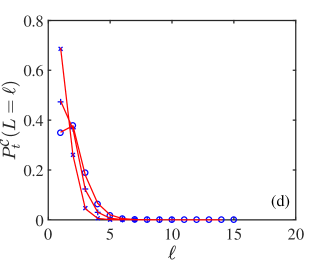
Figure 6: Analytical results (solid lines) for the distribution $P_{t}^{\cal C}(L=\ell)$ of the corded DND network with (a) $p=0.2$; (b) $p=0.4$; (c) $p=0.6$; and (d) $p=0.8$, for network sizes of $N_{t}=10^{2}$, $10^{4}$ and $10^{6}$. The analytical results are found to be in very good agreement with the results of computer simulations (symbols), obtained by averaging over $100$ network instances. As $p$ is increased, the distances become shorter and the DSPL becomes narrower.

6 The mean distance

The mean distance between pairs of nodes in the corded DND networks is obtained by averaging the path lengths among pairs of nodes $i$ and $j$, that are connected by directed paths from $i$ to $j$. It is given by

$${\mathbb{E}}_{t}[L|L<\infty]=\sum_{\ell\geq 1}\ell P_{t}^{\cal C}(L=\ell).$$ (51)

It can also be expressed in the form

$${\mathbb{E}}_{t}[L|L<\infty]=\frac{\sum\limits_{\ell\geq 1}\ell P_{t}(L=\ell)}{P_{t}(L<\infty)}.$$ (52)

Carrying up the summation in the numerator of Eq. (52) we obtain

$${\mathbb{E}}_{t}[L|L<\infty] = \frac{(s+1)P_{0}(L<\infty){\mathbb{E}}_{0}[L|L<\infty]}{(s+1)P_{0}(L<\infty)+\ln t_{s}}$$ (53)

$$+ \frac{\left[1+(1-\eta)(s+1)P_{0}(L<\infty)\right]\ln t_{s}}{(s+1)P_{0}(L<\infty)+\ln t_{s}}$$

$$+ \frac{(1-\eta)(\ln t_{s})^{2}}{2[(s+1)P_{0}(L<\infty)+\ln t_{s}]}$$

The first term on the right hand side of Eq. (53) accounts for the contribution of paths between pairs of nodes that reside on the seed network. The second term accounts for paths from nodes that formed during the growth phase to nodes in the seed network, while the third term accounts for paths between pairs of nodes that formed during growth. At $t=0$ the rescaled time is $t_{s}=1$ and $\ln t_{s}=0$. As a result, the initial value of ${\mathbb{E}}_{t}[L|L<\infty]$ is indeed ${\mathbb{E}}_{0}[L|L<\infty]$. The first term in Eq. (53) decreases monotonically as time proceeds, the second term initially increases and then starts to decrease, while the third term increases monotonically in time. In the long time limit the third term becomes dominant and

$${\mathbb{E}}_{t}[L|L<\infty]\rightarrow\frac{1-\eta}{2}\ln t.$$ (54)

In Fig. 7 we present the mean distance, ${\mathbb{E}}_{t}[L|L<\infty]$, as a function of the network size $N_{t}$, for $p=0.2,0.4,0.6$ and $0.8$. The analytical results, obtained from Eq. (53), where $\eta$ is taken from Eq. (26), are found to be in very good agreement with the results obtained from computer simulations (symbols).

Figure 7: Analytical results (solid lines) for the mean shortest path length ${\mathbb{E}}_{t}[L|L<\infty]$, of the corded DND network, as a function of network size $N_{t}$, obtained from Eq. (53), for $p=0.2$, $0.4$, $0.6$ and $0.8$. The analytical results are in very good agreement with the simulation results (symbols), confirming the logarithmic dependence of ${\mathbb{E}}_{t}[L|L<\infty]$ on the network size. As $p$ is increased, the network becomes more dense and the slope of ${\mathbb{E}}_{t}[L|L<\infty]$ as a function of $\ln N_{t}$ decreases. For clarity, we focus on network sizes in the range $10^{2}\leq N_{t}\leq 10^{6}$.

7 The variance of the DSPL

In order to obtain the variance of the DSPL, we need to calculate its second moment, which is given by

$${\mathbb{E}}_{t}[L^{2}|L<\infty]=\sum_{\ell\geq 1}\ell^{2}P_{t}^{\cal C}(L=\ell).$$ (55)

Carrying out the summations, we obtain

$${\mathbb{E}}_{t}[L^{2}|L<\infty] = \frac{(s+1)P_{0}(L<\infty){\mathbb{E}}_{0}[L^{2}|L<\infty]}{(s+1)P_{0}(L<\infty)+\ln t_{s}}$$ (56)

$$+ \frac{\left[1+(1-\eta)P_{0}(L<\infty)\right]\ln t_{s}}{(s+1)P_{0}(L<\infty)+\ln t_{s}}$$

$$+ \frac{2(1-\eta)P_{0}(L<\infty){\mathbb{E}}_{0}[L|L<\infty]\ln t_{s}}{(s+1)P_{0}(L<\infty)+\ln t_{s}}$$

$$+ \frac{(1-\eta)(5-2\eta)P_{0}(L<\infty)(\ln t_{s})^{2}}{2[(s+1)P_{0}(L<\infty)+\ln t_{s}]}$$

$$+ \frac{(1-\eta)^{2}(\ln t_{s})^{3}}{3[(s+1)P_{0}(L<\infty)+\ln t_{s}]}.$$

The first term on the right hand side of Eq. (56) accounts for paths between pairs of nodes that reside on the seed network. The second and third terms account for paths from nodes that form during growth and nodes in the seed network, while the last two terms account for paths between pairs of nodes that form during growth. Clearly, the initial value of the second moment at $t=0$ is given by ${\mathbb{E}}_{0}[L^{2}|L<\infty]$. As time proceeds the first term decreases monotonically, the second and third terms initially increase and then start to decrease, while the last two terms increase monotonically. In the long time limit

$${\mathbb{E}}_{t}[L^{2}|L<\infty]\rightarrow\frac{1}{3}(1-\eta)^{2}(\ln t)^{2}.$$ (57)

The variance of $P_{t}(L=\ell)$ is given by

$${\rm Var}_{t}(L)={\mathbb{E}}_{t}[L^{2}|L<\infty]^{2}-{\mathbb{E}}_{t}[L|L<\infty]^{2},$$ (58)

where ${\mathbb{E}}[L^{2}|L<\infty]$ is given by Eq. (56) and ${\mathbb{E}}[L|L<\infty]$ is given by Eq. (53). In the long time limit, the variance converges to

$${\rm Var}_{t}(L)=\frac{1}{12}(1-\eta)^{2}(\ln t)^{2}.$$ (59)

In Fig. 8 we present the variance, ${\rm Var}_{t}(L)$, of the DSPL of the corded DND network as a function of network size, $N_{t}$, for $p=0.2,0.4,0.6$ and $0.8$.. The analytical results (solid lines), obtained from Eq. (58), where $\eta$ is taken from Eq. (26), are found to be in good agreement with the results of numerical simulations (symbols), thus the logarithmic scaling is confirmed.

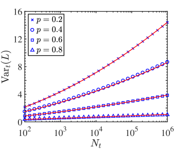
Figure 8: Analytical results (solid lines) for the variance ${\rm Var}_{t}(L)$, of the distribution $P_{t}^{\cal C}(L=\ell)$ of the corded DND network, as a function of network size $N_{t}$, obtained from Eq. (58) for $p=0.2$, $0.4$, $0.6$ and $0.8$. The analytical results are in very good agreement with the simulation results (symbols).

8 Discussion

In an earlier paper we studied the DSPL of a corded ND network model in which the links are undirected. Starting from a single-component seed network, the network maintains its single component structure. In this case any pair of nodes is connected by at least one path. We obtained exact analytical results for the DSPL of this network, which consists of two terms. The first term depends on the DSPL of the seed network and dominates the results at short times, while the second term is independent of the DSPL of the seed network and dominates the results at long times. It was found that the mean distance is given by $\langle L\rangle_{t}\simeq 2(1-\eta)\ln N_{t}$, which means that the resulting network is a small world network. The undirected ND network undergoes a phase transition at $p=1/2$, above which the network becomes extremely dense Lambiotte2016 ; Bhat2016 . As a result, for $p\rightarrow 1/2$ from below, the shortest paths become highly degenerate, in the sense that most pairs of nodes are connected by several shortest paths, which all have the same length.

The corded DND model differs from its undirected counterpart is several ways. Unlike the undirected model in which D may form probabilistic links to all the neighbors of M, in the directed model it may form (directed) probabilistic links only to the outgoing neighbors of M and not to the incoming neighbors of M. In the undirected network each pair of nodes is connected by at least one path. In contrast, from each node in the directed network one can access only older nodes which reside along the branch of the backbone tree which leads to the sink node. As a result, the probability that a random pair of nodes are connected by a directed path is $P_{t}(L<\infty)\simeq\ln N_{t}/N_{t}$. However, the mean distance between pairs of nodes which are connected by directed paths exhibits the same qualitative behavior as in the undirected network, namely ${\mathbb{E}}_{t}[L|L<\infty]\simeq[(1-\eta)/2]\ln N_{t}$.

The corded DND model may be useful in the study of scientific citation networks. In these networks each new paper emanates from one or more papers which were previously published in the literature. The earlier papers, which are cited in the new paper, are analogous to the mother node in the corded DND network. More specifically, each paper is represented by a node and each citation is represented by a directed link from the citing paper to the cited paper. The in-degree of each node is the number of citations received by the corresponding paper, while the out-degree is the number of papers that appear in the reference list at the end of the paper. Clearly, the out-degree of a paper is easily accessible and is fixed once the paper is published. In contrast, the in-degree of a paper is initially zero and it may grow as the paper gets cited by subsequent papers. The citations of each paper are spread throughout the scientific literature. Gathering this information requires an effort. It can be obtained from search engines such as the Institute of Scientific Information (ISI) Web of Knowledge and Google Scholar.

The corded DND model captures some essential properties of scientific citation networks. It is a directed network whose links point from the citing paper to the cited paper. The probabilistic links from the daughter node to outgoing neighbors of the mother node correspond to the fact that a citation of a paper is often accompanied by citations to some of the earlier papers that appear in its reference list. These probabilistic links also invoke the preferential attachment mechanism, because the probability of a node to receive such link is proportional to its in-degree. This is the mechanism that gives rise to the power-law tail of the in-degree distribution. The shift in the power-law degree distribution is due to the fact that the deterministic links are formed by random attachment with no preference to high degree nodes.

The corded DND network provides some insight on the structure of the scientific citation networks. In particular, it indicates that for a given paper, the typical number of papers that are connected to it by directed paths of citations (in the past or future) scales like $\ln N/N$, where $N$ is the network size. This implies that the scientific literature is highly fragmented in the sense that most pairs of papers are not connected via chains of citations and thus the network is not a small-world network. For those pairs of papers that are connected by chains of subsequent citations, the DSPL provides the breakdown into direct citations, indirect citations via a single intermediate paper and indirect citations of higher orders. This sheds new light on the way the impact of a paper may be evaluated, namely not only in terms of the direct citations but also in terms of the cumulative effect of all the secondary citations. Another aspect revealed by the model is that the structure of citation networks evolves slowly, with a typical time scale which is logarithmic in the network size. This is in spite of the random nature of the growth process. However, it should be emphasized that the corded DND model should be considered as a minimal model of citation networks. In more complete models a new paper may cite several ’mother nodes’ as well as some of the earlier papers cited in them. This would increase the number of directed paths but is not expected to change the qualitative properties of the network.

9 Summary

We obtained exact analytical results for the time dependent DSPL in a model of directed network that grows by a node duplication mechanism. In this model, at each time step a random mother node is duplicated. The daughter node acquires a directed link to the mother node, and with probability $p$ it acquires a directed link to each one of the outgoing neighbors of the mother node. To obtain the DSPL we derived a master equation for the time evolution of the probability $P_{t}(L=\ell)$. Finding an exact analytical solution of the master equation, we obtained a closed form expression for the DSPL, in which the probability $P_{t}(L=\ell)$ is expressed as a sum of two terms. The first term is a convolution between the DSPL of the seed network, $P_{0}(L=\ell)$, and a Poisson distribution. The second term is a sum of Poisson distributions. The expression for $P_{t}(L=\ell)$ is valid at all times and is not merely an asymptotic result. We calculated the mean distance between pairs of nodes that are connected by directed paths and showed that in the long time limit it scales like ${\mathbb{E}}_{t}[L|L<\infty]\simeq\frac{1-\eta}{2}\ln N_{t}$. Thus, the mean distance between pairs of nodes that are connected by directed paths scales logarithmically with the network size, as in small-world networks. However, the fraction of pairs of nodes that are connected by directed paths diminishes like $\ln N_{t}/N_{t}$ as the network size increases, while most pairs of nodes are not connected by directed paths. Therefore, the corded DND network is not a small-world network, unlike the corded undirected node duplication network.

Acknowledgements

This work was supported by the Israel Science Foundation grant no. 1682/18.

Author contribution statement

All three authors contributed at all stages of the project.

Appendix A Canonical set of configurations and the degeneracies of shortest paths

In the master equation, $\vec{P}_{t}^{\rm D}(G=g)=T\vec{P}_{t}^{\rm M}(G=g)$, that describes the evolution of the degeneracies of shortest paths from mother to daughter nodes, we use a canonical set of downstream configurations. The low level configurations in this set are shown in Fig. 3. In addition to the canonical configurations, the duplication step may lead to configurations which are not included in the canonical set. Each one of these configurations is equivalent to a specific canonical configuration in the sense that they both exhibit the same level of degeneracy of the shortest paths from the newly formed node, D, to upstream nodes. To illustrate this property, we present in Fig. 9(a) the configuration obtained upon duplication of a node, M, of configuration $g=1^{**}$, in which neither of the two outgoing links of M was duplicated. The degeneracy of the shortest paths from D to downstream nodes is $g=1$. Due to the shortcut from M to GGM, none of these shortest paths goes through GM. Therefore, the betweeness centrality of GM is $0$. Moreover, GM is not directly connected to D and thus it cannot gain new incoming links upon duplication of D. Thus, the node GM has no effect on the degeneracy of the shortest paths from D (and its descendants) to downstream nodes. It can thus be deleted, as shown in Fig. 9(a), giving rise to a canonical configuration of the form $g=1^{*}$. In Fig. 9(b) we present a configuration obtained from the duplication of a node M for which $g_{\rm M}=1^{**}$. In this case, the link to GGM was duplicated while the link to GM was not duplicated. In this case none of the shortest paths from D to upstream nodes go through GM and it can thus be deleted, giving rise to the canonical configuration $g_{\rm D}=1^{**}$.

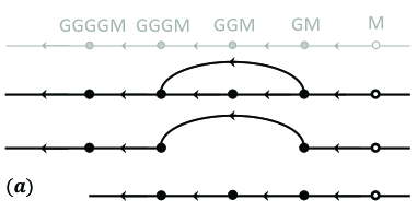
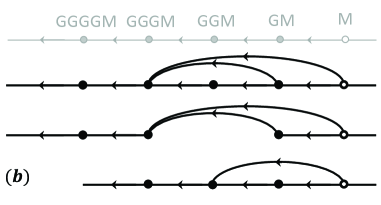
Figure 9: (a) The configuration obtained upon duplication of a node M of configuration $g_{\rm M}=1^{**}$, in which neither of the two outgoing links of M was duplicated. The degeneracy of the shortest paths from D to downstream nodes is $g=1$. Due to the shortcut from M to GGM, none of these shortest paths goes through GM. Moreover, GM is not directly connected to D and thus it cannot gain new incoming links upon duplication of D. Thus, the node GM has no effect on the degeneracy of the shortest paths from D (and its descendants) to downstream nodes. Thus, its deletion has no effect on these shortest paths and their degeneracies. The deletion of the node GM results in a canonical configuration of the form $g_{\rm D}=1^{*}$; (b) A configuration obtained from the duplication of a node M for which $g_{\rm M}=1^{**}$, where the link to GGM was duplicated while the link to GM was not duplicated. In this case none of the shortest paths from D to upstream nodes go through GM and it can thus be deleted, giving rise to the canonical configuration $g_{\rm D}=1^{**}$.

Appendix B Master equation for the degeneracies

In order to analyze the temporal evolution of the degeneracies, we derive below the master equation for the distribution of degeneracy levels. For simplicity, we consider the case of single and double degeneracies, in which the distribution $\vec{P}_{t}(G=g)$ is given by Eq. (6) and the transition matrix, $T$ is given by Eq. (7). The degeneracy distribution of the daughter node, which is formed at time $t$, is given by

$$P_{t}^{\rm D}(G=1^{*}) = (1-p)P_{t}^{\rm M}(G=1^{*})$$

$$+ (1-p)^{2}P_{t}^{\rm M}(G=1^{**})$$

$$+ (1-p)^{2}P_{t}^{\rm M}(G=2)$$

$$P_{t}^{\rm D}(G=1^{**}) = pP_{t}^{\rm M}(G=1^{*})+pP_{t}^{\rm M}(G=1^{**})$$

$$+ 2p(1-p)P_{t}^{\rm M}(G=2)$$

$$P_{t}^{\rm D}(G=2) = p(1-p)P_{t}^{\rm M}(G=1^{**})$$ (B.1)

$$+ p^{2}P_{t}^{\rm M}(G=2)$$

The degeneracy distribution at time $t+1$ is given by

$$\vec{P}_{t+1}(G=g)=\frac{N_{t}\vec{P}_{t}(G=g)+\vec{P}_{t}^{\rm D}(G=g)}{N_{t}+1},$$ (B.2)

where $g=1^{*},1^{**}$ and $2$. Inserting $\vec{P}_{t}^{\rm D}(G=g)$ from Eq. (B.1) into Eq. (B.2), subtracting $\vec{P}_{t}(G=g)$ from both sides and replacing the difference on the left hand side by a time derivative, we obtain

$$\frac{d}{dt}P_{t}(G=1^{*}) = \frac{-pP_{t}(G=1^{*})}{N_{t}+1}$$

$$+ \frac{(1-p)^{2}[P_{t}(G=1^{**})+P_{t}(G=2)]}{N_{t}+1}$$

$$\frac{d}{dt}P_{t}(G=1^{**}) = \frac{pP_{t}(G=1^{*})-(1-p)P_{t}(G=1^{**})}{N_{t}+1}$$

$$+ \frac{2p(1-p)P_{t}(G=2)}{N_{t}+1}$$

$$\frac{d}{dt}P_{t}(G=2) = \frac{p(1-p)P_{t}(G=1^{**})}{N_{t}+1}$$ (B.3)

$$- \frac{(1-p)^{2}P_{t}(G=2)}{N_{t}+1}.$$

The solution of this master equation is given by

$$P_{t}(G=1^{*}) = \frac{(1-p)^{2}}{1-p+p^{2}}+\frac{P_{0}(G=1^{*})}{t_{s}^{1-p+p^{2}}}$$

$$- \frac{(1-p)^{2}}{(1-p+p^{2})t_{s}^{1-p+p^{2}}}$$

$$P_{t}(G=1^{**}) = \frac{p(1+p)}{(1+2p)(1-p+p^{2})}$$

$$- \frac{(1-2p)P_{0}(G=1^{*})}{(2-3p)t_{s}^{1-p+p^{2}}}$$

$$+ \frac{(1-2p)(1-p)^{2}}{(2-3p)(1-p+p^{2})t_{s}^{1-p+p^{2}}}$$

$$+ \frac{(1-2p)P_{0}(G=1^{*})}{(2-3p)t_{s}^{1+p-2p^{2}}}+\frac{P_{0}(G=1^{**})}{t_{s}^{1+p-2p^{2}}}$$

$$- \frac{1+p-4p^{2}}{(1+2p)(2-3p)t_{s}^{1+p-2p^{2}}}$$

$$P_{t}(G=2) = \frac{p^{2}}{(1+2p)(1-p+p^{2})}$$ (B.4)

$$- \frac{(1-p)P_{0}(G=1^{*})}{(2-3p)t_{s}^{1-p+p^{2}}}$$

$$- \frac{(1-p)^{2}}{(1-p+p^{2})t_{s}^{1-p+p^{2}}}$$

$$+ \frac{1+p-4p^{2}}{(1+2p)(2-3p)t_{s}^{1+p-2p^{2}}}$$

$$- \frac{(1-2p)P_{0}(G=1^{*})}{(2-3p)t_{s}^{1+p-2p^{2}}}$$

$$- \frac{P_{0}(G=1^{**})}{t_{s}^{1+p-2p^{2}}}.$$

The convergence of the degeneracy distribution, $P_{t}(G=g)$ to its asymptotic form follows a power-law function of the time with the two exponents:

$$\alpha_{1} = 1-p+p^{2}$$

$$\alpha_{2} = 1+p-2p^{2}.$$ (B.5)

The degeneracy distribution at steady state conditions is given by

$$P(G=1^{*}) = \frac{(1-p)^{2}}{1-p+p^{2}}$$

$$P(G=1^{**}) = \frac{p(1+p)}{(1+2p)(1-p+p^{2})}$$

$$P(G=2) = \frac{p^{2}}{(1+2p)(1-p+p^{2})}.$$ (B.6)

The convergence rate to steady state is dominated by the smaller exponent among $\alpha_{1}$ and $\alpha_{2}$, namely $\alpha_{\rm min}=\min\{\alpha_{1},\alpha_{2}\}$. One can show that for $p<2/3$, $\alpha_{\rm min}=\alpha_{1}$, while for $p>2/3$, $\alpha_{\rm min}=\alpha_{2}$. The time its takes for the difference $\Delta P_{t}(G=g)=P_{t}(G=g)-P(G=g)$ to go down to $1/e$ of its initial value is given by

$$\tau=(s+1)\left[e^{1/\alpha_{\rm min}}-1\right].$$ (B.7)

In the limit of $p\rightarrow 1^{-}$ the exponent $\alpha_{2}$ satisfies $\alpha_{2}\rightarrow 0$. As a result, the convergence slows down as $p$ is increased towards $p=1$.

Appendix C Exact form of the master equation

In the derivation of the master equation for $P_{t}(L=\ell)$, where $\ell=1,2$, we used an approximation in which we replaced the probability $p$ by $\eta$ in Eqs. (37) and (38). Here we present the exact master equation, obtained from Eqs. (35) and (22), in case that $p$ is not replaced by $\eta$. In this case, the equation for $P_{t}(L=1)$ takes the form

$$\frac{d}{dt}P_{t}(L=1) = -\left(\frac{2-p}{t+s+1}\right)P_{t}(L=1)$$ (C.1)

$$+ \frac{1}{(t+s+1)^{2}},$$

which is similar to Eq. (41) except for the replacement of $\eta$ by $p$. The equation for $P_{t}(L=2)$ takes the form

$$\frac{d}{dt}P_{t}(L=2) = -\left(\frac{2-\eta}{t+s+1}\right)P_{t}(L=2)$$ (C.2)

$$+ \left(\frac{1-p}{t+s+1}\right)P_{t}(L=1),$$

which is similar to Eq. (47), except for the replacement of $\eta$ by $p$ in the second term on the right hand side. The time derivatives of $P_{t}(L=\ell)$ for $\ell\geq 3$ are given by Eq. (47) and the time derivative of $P_{t}(L=\infty)$ is given by Eq. (31). The solution for $P_{t}(L=1)$ is given by

$$P_{t}(L=1) = \frac{1}{t_{s}^{2-p}}\left[P_{0}(L=1)-\frac{1}{(1-p)(s+1)}\right]$$ (C.3)

$$+ \frac{1}{(1-p)(s+1)t_{s}},$$

which is similar to Eq. (42), except for the replacement of $\eta$ by $p$. The solution for $P_{t}(L=\ell)$, $\ell\geq 2$ is given by

$$P_{t}(L=\ell) = \frac{(1-p)}{t_{s}^{2-\eta}}\frac{(1-\eta)^{\ell-2}(\ln t_{s})^{\ell-1}}{(\ell-1)!}P_{0}(L=1)$$ (C.4)

$$+ \frac{1-p}{t_{s}^{2-\eta}}\left(\frac{1-\eta}{p-\eta}\right)^{\ell-2}\times$$

$$\ \ \ \ \ \ \sum_{\ell^{\prime}=\ell}^{\infty}\frac{(p-\eta)^{\ell^{\prime}-1}(\ln t_{s})^{\ell^{\prime}}}{\ell^{\prime}!}P_{0}(L=1)$$

$$+ \frac{1}{t_{s}^{2-\eta}}\sum_{\ell^{\prime}=2}^{\min\{\ell,\Delta_{0}\}}\frac{[(1-\eta)\ln t_{s}]^{\ell-\ell^{\prime}}}{(\ell-\ell^{\prime})!}P_{0}(L=\ell^{\prime})$$

$$- \frac{1}{t_{s}^{2-\eta}}\left(\frac{1-\eta}{p-\eta}\right)^{\ell-2}\sum_{\ell^{\prime}=\ell}^{\infty}\frac{(p-\eta)^{\ell^{\prime}-1}(\ln t_{s})^{\ell^{\prime}}}{(s+1)\ell^{\prime}!}$$

$$+ \frac{1}{t_{s}^{2-\eta}}\sum_{\ell^{\prime}=\ell}^{\infty}\frac{(1-\eta)^{\ell^{\prime}-1}(\ln t_{s})^{\ell^{\prime}}}{(s+1)\ell^{\prime}!}.$$

The first two terms on the right hand side of Eq. (C.4) correspond to the first term of Eq. (48), except that in the contribution of $P_{0}(L=1)$ is multiplied by $(1-p)/(1-\eta)$. These terms account for the components of $P_{t}(L=\ell)$ that depend on the DSPL of the seed network. The third term adjusts for the difference between $p$ and $\eta$ in the terms that depend on the DSPL of the seed network. The fourth term corresponds to the second term of Eq. (48), which does not depend on the DSPL of the seed network. The last term adjusts for the difference between $p$ and $\eta$ in the terms that do not depend on the DSPL of the seed network. The results for $P_{t}(L=\infty)$ are given by Eq. (32).

References

- (1) R. Albert, A.-L. Barabási, Rev. Mod. Phys. 74, 47 (2002)
- (2) G. Caldarelli, Scale free networks: complex webs in nature and technology (Oxford University Press, 2007)
- (3) S. Havlin, R. Cohen, Complex Networks: Structure, Robustness and Function (Cambridge University Press, 2010)
- (4) M.E.J. Newman, Networks: an Introduction (Oxford University Press, 2010)
- (5) E. Estrada, The Structure of Complex Networks: Theory and Applications (Oxford University Press, 2011)
- (6) A. Barrat, M. Barthélemy, A. Vespignani, Dynamical Processes on Complex Networks (Cambridge University Press, 2012)
- (7) S. Milgram, Psychology Today 1, 61 (1967)
- (8) D. Watts, S. Strogatz, Nature 393, 440 (1998).
- (9) F. Chung, L. Lu, Proc. Nat. Acad. Sci. USA 99, 15879 (2002)
- (10) F. Chung, L. Lu, Internet Mathematics 1, 91 (2003)
- (11) A.-L. Barabási, R. Albert, Science 286, 509 (1999)
- (12) H. Jeong, B. Tombor, R. Albert, Z.N. Oltvai, A.-L. Barabási, Nature 407, 651 (2000)
- (13) P.L. Krapivsky, S. Redner, F. Leyvraz, Phys. Rev. Lett. 85, 4629 (2000)
- (14) P.L. Krapivsky, S. Redner, Phys. Rev. E 63, 066123 (2001)
- (15) A. Vázquez, Phys. Rev. E 67, 056104 (2003)
- (16) R. Cohen, S. Havlin, Phys. Rev. Lett. 90, 058701 (2003)
- (17) L. Giot et al., Science 302 1727 (2003)
- (18) A. Maáyan, S.L. Jenkins, S. Neves, A. Hasseldine, E. Grace, B. Dubin-Thaler, N.J. Eungdamrong, G. Weng, P.T. Ram, J.J. Rice, A. Kershenbaum, G.A. Stolovitzky, R.D. Blitzer, R. Iyengar, Science 309, 1078 (2005)
- (19) E.W. Dijkstra, Numerische Mathematik 1, 269 (1959)
- (20) D. Delling, P. Sanders, D. Schultes, D. Wagner, Engineering route planning algorithms, in Algorithmics of large and complex networks: design, analysis, and simulation, J. Lerner, D. Wagner, and K.A. Zweig (Eds.), p. 117 (2009)
- (21) R. Pastor-Satorras, C. Castellano, P. Van Mieghem, A. Vespignani, Rev. Mod. Phys. 87, 925 (2015)
- (22) B. Bollobas, Random Graphs, Second Edition (Academic Press, London, 2001)
- (23) R. Durrett, Random Graph Dynamics (Cambridge University Press, Cambridge, 2007)
- (24) A. Fronczak, P. Fronczak, J.A. Holyst, Phys. Rev. E 70, 056110 (2004)
- (25) M.E.J. Newman, Proc. Natl. Acad. Sci. USA 98, 404 (2001)
- (26) A.K. Hartmann, M. Mézard, Phys. Rev. E 97, 032128 (2017)
- (27) M.E.J. Newman, S.H. Strogatz, D.J. Watts, Phys. Rev. E 64, 026118 (2001)
- (28) S.N. Dorogotsev, J.F.F. Mendes, A.N. Samukhin, Nuclear Physics B 653, 307 (2003)
- (29) V.D. Blondel, J.-L. Guillaume, J.M. Hendrickx, R.M. Jungers, Phys. Rev. E 76, 066101 (2007)
- (30) R. van der Hofstad, G. Hooghiemstra, D. Znamenski, Electronic Journal of Probability 12, 703 (2007)
- (31) H. van der Esker, R. van der Hofstad, G. Hooghiemstra, J. Stat. Phys. 133, 169 (2008)
- (32) J. Shao, S. V. Buldyrev, R. Cohen, M. Kitsak, S. Havlin, H. E. Stanley, Europhys. Lett. 84, 48004 (2008)
- (33) J. Shao, S.V. Buldyrev, L.A. Braunstein, S. Havlin, H.E. Stanley, Phys. Rev. E 80, 036105 (2009)
- (34) E. Katzav, M. Nitzan, D. ben-Avraham, P.L. Krapivsky, R. Kühn, N. Ross, O. Biham, EPL 111, 26006 (2015)
- (35) P. Erdős, A. Rényi, Publicationes Mathematicae (Debrecen) 6, 290 (1959)
- (36) P. Erdős, A. Rényi, Publ. Math. Inst. Hung. Acad. Sci. 5, 17 (1960)
- (37) P. Erdős, A. Rényi, Bull. Inst. Int. Stat. 38, 343 (1961)
- (38) M. Nitzan, E. Katzav, R. Kühn, O. Biham, Phys. Rev. E 93, 062309 (2016)
- (39) S. Melnik, J.P. Gleeson, arXiv:1604.05521
- (40) M. Molloy, B. Reed, Random Struct. Algorithms 6, 161 (1995)
- (41) M. Molloy, B. Reed, Combinatorics, Probability and Computing 7 , 295 (1998)
- (42) A. Bhan, D.J. Galas, T.G. Dewey, Bioinformatics 18, 1486 (2002)
- (43) J. Kim, P.L. Krapivsky, B. Kahng, S. Redner, Phys. Rev. E 66, 055101 (2002)
- (44) F. Chung, L. Lu, T.G. Dewey, D.J. Galas, J. Comput. Biol. 10, 677 (2003)
- (45) P.L. Krapivsky, S. Redner, Phys. Rev. E 71, 036118 (2005)
- (46) I. Ispolatov, P.L. Krapivsky, A. Yuryev, Phys. Rev. E 71, 061911 (2005)
- (47) I. Ispolatov, P.L. Krapivsky, I. Mazo, A. Yuryev, New J. Phys. 7, 145 (2005)
- (48) G. Bebek, P. Berenbrink, C. Cooper, T. Friedetzky, J. Nadeau, S.C. Sahinalp, Theor. Comput. Sci. 369, 239 (2006)
- (49) S. Li, K.P. Choi, T. Wu, Theor. Comput. Sci. 476, 94 (2013)
- (50) R. Lambiotte, P.L. Krapivsky, U. Bhat, S. Redner, Phys. Rev. Lett. 117, 218301 (2016)
- (51) U. Bhat, P.L. Krapivsky, R. Lambiotte, S. Redner, Phys. Rev. E. 94, 062302 (2016)
- (52) R. Toivonen, L. Kovanen, M. Kivelä, J.-P. Onnela, J. Saramäki, K. Kaski, Social Networks 31, 240 (2009)
- (53) M. Granovetter, American Journal of Sociology 78, 1360 (1973)
- (54) R. Milo, S. Shen-Orr, S. Itzkovitz, N. Kashtan, D. Chklovskii, U. Alon, Science 298, 824 (2002)
- (55) U. Alon, An Introduction to Systems Biology: Design Principles of Biological Circuits (Chapman and Hall/CRC, 2006)
- (56) C. Steinbock, O. Biham, E. Katzav, Phys. Rev. E 96, 032301 (2017)
- (57) S. Ohno, Evolution by Gene Duplication (Springer-Verlag, New York, 1970)
- (58) S.A. Teichmann, M.M. Babu, Nature Genetics 36, 492 (2004)
- (59) S. Redner, Eur. Phys. J. B 4, 131 (1998)
- (60) S. Redner, Physics Today 58, 49 (2005)
- (61) F. Radicchi, S. Fortunato, C. Castellano, Proc. Natl. Acad. Sci. USA 105, 17268 (2008)
- (62) M. Golosovsky, S. Solomon, Phys. Rev. Lett. 109, 098701 (2012)
- (63) M. Golosovsky and S. Solomon, Phys. Rev. E 95, 012324 (2017)
- (64) M. Golosovsky, Phys. Rev. E 96, 032306 (2017)
- (65) G.J. Peterson, Steve Pressé, K.A. Dill, Proc. Natl. Acad. Sci. USA 107 , 16023 (2010)
- (66) C. Steinbock, O. Biham, E. Katzav, J. Stat. Mech. 083403 (2019).
- (67) R.T. Smythe, H. Mahmoud, Theory Probab. Math. Statist. 51, 1 (1995)
- (68) M. Drmota, B. Gittenberger, Random Struct. Alg. 10, 421 (1997)
- (69) M. Drmota, H.-K. Hwang, Adv. Appl Probab. 37, 321 (2005)