The K2 Bright Star Survey I: Methodology and Data Release

Abstract

While the Kepler  Mission was designed to look at tens of thousands of faint stars ($V\gtrsim 12$), brighter stars that saturated the detector are important because they can be and have been observed very accurately by other instruments. By analyzing the unsaturated scattered-light ‘halo’ around these stars, we have retrieved precise light curves of most of the brightest stars in K2 fields from Campaign 4 onwards. The halo method does not depend on the detailed cause and form of systematics, and we show that it is effective at extracting light curves from both normal and saturated stars. The key methodology is to optimize the weights of a linear combination of pixel time series with respect to an objective function. We test a range of such objective functions, finding that lagged Total Variation, a generalization of Total Variation, performs well on both saturated and unsaturated K2 targets. Applying this to the bright stars across the K2 Campaigns reveals stellar variability ubiquitously, including effects of stellar pulsation, rotation, and binarity. We describe our pipeline and present a catalogue of the 161 bright stars, with classifications of their variability, asteroseismic parameters for red giants with well-measured solar-like oscillations, and remarks on interesting objects. These light curves are publicly available as a High Level Science Product from the Mikulski Archive for Space Telescopes (MAST).

ʻ ‘

1 Introduction

The Kepler Space Telescope was launched with a main goal of determining the frequency of Earth-sized planets around Solar-like stars (Borucki et al., 2010). In order to explore these populations it was necessary to observe hundreds of thousands of stars, with the consequence that the Kepler exposure time and gain were set to optimally observe eleventh or twelfth-magnitude stars, while bright stars are saturated and intentionally avoided. In the two-wheeled revival as the K2 mission, the Kepler telescope observed a sequence of ecliptic-plane fields containing many more very-saturated stars (Howell et al., 2014). While it is difficult to obtain precise light curves of these stars because of their saturation, they are some of the most valuable targets to follow up with photon-hungry methods such as interferometry and high-resolution spectroscopy, and they typically have long histories of previous observations. Dedicated bright-star space photometry missions such as MOST (Walker et al., 2003) and the BRITE-Constellation (Weiss et al., 2014; Pablo et al., 2016) use very small telescopes (15 cm and 3 cm apertures respectively), to assemble time-series photometry of bright stars, but larger telescopes such as Kepler (0.95 m) lead to higher-precision light curves.

The Kepler detector saturates at a magnitude of $K_{p}\sim 11.3$ in both long- (30 min) and short (1 min)-cadence data, since these both represent sums of 6 s exposures (Gilliland et al., 2010). For objects brighter than this, excess electrons ‘bleed’ into adjacent pixels in both directions along the column containing the star. Simple aperture photometry (SAP) – adding all the flux contained in a window around the bleed column – has recovered light curves with precisions close to the photon noise limit. Examples treated in the nominal Kepler mission are the prototype classical radial pulsator RR Lyr ($V=7.2$; Kolenberg et al., 2011), the solar-like pulsators 16 Cyg AB ($V\approx 6$; Metcalfe et al., 2012; White et al., 2013; Metcalfe et al., 2015) and $\theta\,$Cyg ($V=4.48$; Guzik et al., 2016), and the massive eclipsing binary V380 Cyg ($V=5.68$; Tkachenko et al., 2014). In the nominal Kepler mission SAP was only attempted for a few bright stars, and in K2 , the larger-amplitude spacecraft motion significantly increased the size of the required apertures for SAP photometry of very saturated stars, while also making their instrumental systematics more difficult to deal with. While the second-version pixel-level-decorrelation (PLD) pipeline EVEREST 2.0 was able to correct systematics in saturated SAP photometry (Luger et al., 2018), this is not possible for the very brightest stars whose bleed columns may run to the edge of the detector. Furthermore, bandwidth constraints meant that pixel data were not downloaded for many bright targets in K2 .

In order to recover precise light curves of the brightest stars in K2 , we have therefore developed two main approaches, ‘smear’ and ‘halo’ photometry. Smear photometry (Pope et al., 2016b, 2019) uses collateral ‘smear’ calibration data to obtain a 1-D spatial profile with $\sim 1/1000$ of the flux on each CCD. This can be processed to recover light curves of stars that were not necessarily conventionally targeted and downloaded with active pixels, because smear data are recorded for all columns. The main disadvantage of this method is that it confuses all stars in the same column, which means that in crowded fields smear light curves tend to be significantly contaminated.

The more precise method of halo photometry, which is the subject of this paper, uses the broad ‘halo’ of scattered light around a saturated star to recover relative photometry, by constructing a light curve as a linear combination of individual pixel time series and minimizing a Total Variation objective function (TV-min). It has been employed for example on the Pleiades (White et al., 2017) and the brightest-ever star on Kepler silicon, Aldebaran ($\alpha$ Tau; Farr et al., 2018), recovering photometry with a precision close to that normally obtained from K2 observations of unsaturated stars. Unlike smear, this requires downloading data out to a 12–20 pixel radius around each star, and has accordingly only been possible for stars that were specifically proposed and targeted with apertures optimized for this method, plus a small number of other stars for which this is fortuitously the case. The pixel requirements for this are sufficiently low that, with the help of the K2 Guest Observer office, such apertures were obtained for most of the bright targets from Campaign 4 onwards.

In this Paper we describe numerical experiments testing the TV-min method and extending it to generalizations with different exponents and timescales. We show that the method as previously employed applying standard TV-min is suboptimal, and gain a modest improvement from taking finite differences close to the timescale of K2 thruster firings. We also document the main changes in the halo data reduction pipeline, halophot, with respect to previous releases. We go on to present a complete catalog of long-cadence K2 halo light curves, which we have made publicly available. We have employed halo photometry on all stars targeted with appropriate apertures, and have done a preliminary characterization of interesting astrophysical variability. These include oscillating red giants, pulsating and quiet main-sequence stars, and eclipsing binaries, many of which are among the brightest objects of their type to have been observed with high-cadence space photometry. We are convinced that this diverse catalog of high-precision light curves will be useful for a range of astrophysical investigations.

2 Halo Photometry Method

The ‘TV-min’ halo method was first described by White et al. (2017) and applied to the Pleiades’ Seven Sisters. It was also applied to Aldebaran with further developments by Farr et al. (2018). In this Section we will discuss some improvements made to the halo method since those publications, and describe tests of the method using saturated and unsaturated targets.

We follow the Optimized-Weight Linear (OWL) photometry concept described by Hogg & Foreman-Mackey (2014, unpublished: preprint github.com/davidwhogg/OWL/) in our assumptions. We assume that a star has a wide PSF sampled by many pixels with different sensitivities. This PSF varies at most to a small extent in time. The star moves around on the detector within a small region. We assume that our time series consists of many epochs sampled with a nearly even cadence. We do not wish to rely on metadata describing the spacecraft motion, pixel gains, PSF variations or other noise processes, at least at this stage.

Because photometry is a linear operation, any estimator of the flux is necessarily a weighted sum of pixel values. We choose these weights to be time-invariant but note that this strong constraint is not necessary in general. Allowing these weights to vary in time is a possible extension of this method to non-stationary noise processes, but we do not explore this further in this work. In OWL and here, we search for a linear combination of pixels that is invariant with respect to the the noise processes but accurately preserved astrophysical signals.

The additional constraint beyond the OWL axioms is that some pixels are saturated, so that Simple Aperture Photometry (SAP) is inadvisable. Instead the measurements are made using the unsaturated pixels at the wings of the broad and structured PSF, with counts $p_{ij}$ where pixels are indexed by $j$ and epoch by $i$. We construct a light curve as a linear combination of these time series with weights $w_{j}$, so that flux $f_{i}$ at epoch $i$ is

$$f_{i}\equiv\sum_{j}{w_{j}p_{ij}}.$$ (1)

In our updated pipeline presented here, the weights are chosen to minimize an objective function

$$Q_{k,\delta}\equiv{\sum_{i>\delta}{|f_{i}-f_{i-\delta}|^{k}}},$$ (2)

with an integer lag parameter $\delta$ and an integer $L_{k}$ norm, subject to the constraints

$$\forall_{j}w_{j} >0$$ (3)

$$\sum_{i=1}^{N}f_{i} =N.$$ (4)

This is a classic convex optimization program with constraints, which we solve with the scipy (Jones et al., 2001) L-BFGS-B nonlinear optimization code (Zhu et al., 1999). $Q_{k,\delta}$ has analytic derivatives with respect to $w_{j}$ (calculated with autograd; Maclaurin et al., 2015), and it is therefore extremely fast to optimize and converges well on a global solution. In practice, for computational reasons we optimize over parameters $\tilde{w}_{j}$ such that $w_{j}=\text{softmax}(\tilde{w}_{j})=\exp{\tilde{w}_{j}}/\sum_{j}(\exp{\tilde{w}_{j}})$, where softmax is the normalized exponential function. This satisfies the constraint that $\forall_{j}w_{j}>0$, and while this also constrains their sum to be unity, we renormalize $f$ to satisfy its normalization constraint before calculating the objective function and this additional constraint is removed again. Weight maps displayed in Figures 3, 10 and 9 display $w_{j}$ and not $\tilde{w}_{j}$.

The objective function $Q_{k,\delta}$ is the $L_{k}$ norm on a ‘lagged’ finite difference with a lag parameter $\delta$. For $k=1$ and $\delta=1$, $Q_{1,1}$ is the standard Total Variation objective (TV) used in previous halo papers (e.g. White et al., 2017; Farr et al., 2018), and can be seen as the L1 norm on the derivative of $f$ or as a discrete approximation to its arc length. The L2 Variation (L2V) with $k=2$ is sometimes referred to in image processing literature as the ‘smoothness’ regularizer, as it seeks to penalize large gradients without necessarily making them sparse. While $k$ does not have to be an integer in principle, in this implementation we have chosen to restrict our analysis to $k\in\{1,2,3\}$. The lag parameter $\delta$ allows for flexibility in modelling systematics occurring at different timescales from epoch-to-epoch, and we investigate its effects below. The order parameter $k$ allows for flexibility in how sensitive we are to normally-distributed versus long-tailed noise. For convenience in the rest of this paper, we will refer to the $k=1$ case as TV, the $k=2$ case as L2V, and the $k=3$ case as L3V. As the sampling in K2 is close to uniform but not perfectly uniform, some finite differences actually skip two or three cadences, but these are a small contribution to the final objective function; for very irregularly sampled data, it may be valuable to interpolate onto a uniform grid.

Parker et al. (2019) in their work on the saturated K2 observations of Titan optimized an objective function equivalent to $Q_{2,1}$ with a second-order finite difference $2f_{i}-f_{i-1}-f_{i+1}$, noting that first-order differences are sensitive to linear trends while second-order differences are invariant. We nevertheless choose to use a first-order finite difference, on the grounds that long-term astrophysical trends on the timescale of a K2 Campaign cannot be straightforwardly distinguished from systematics, and that the short-timescale noise performance of optimizing $Q_{2,1}$ with respect to first-order differences was superior in our numerical experiments.

Unlike other methods for calibrating Kepler systematics, other than the value of $\delta$, no knowledge of the spacecraft motion or the behaviour of an ensemble of other stars is used to inform our algorithm. The signal and the noise are jointly estimated from the data. The method is both self-calibrating, and is independent of the details of the systematics it is calibrating, operating on the assumption that a single signal is present across many individual time series which otherwise are contaminated by noise.

It is therefore likely that significant improvements can be made to the method by including cotrending basis vectors with mean zero and whose weights are allowed to be negative, which would represent systematics which are common to all pixels in the halo aperture and therefore masquerade as signal. Any linear combination of convex objective functions is itself convex, and future extensions to the method could apply combinations of different lags and orders to better represent systematics occurring on different timescales (e.g. thruster firings, red noise) and with different levels of smoothness.

In addition to expanding the range of possible objective functions, we have also added a feature ‘deathstar’ to deal with contamination. Clusters of pixels are identified with the dbscan algorithm (Density-Based Spatial Clustering of Applications with Noise; Ester et al., 1996), and we join these clusters with the watershed-based image segmentation algorithm from k2p2 (Lund et al., 2015). Clusters other than the target star identified by this algorithm are identified as possible background sources and removed from the target pixel file before processing. Other than this, we have adopted less-aggressive quality flagging, having found that many epochs were being classified as bad quality for spurious ‘cosmic ray’ events, which were actually caused by a combination of saturation and spacecraft motion. We instead chose to iteratively sigma-clip outliers and use the lightkurve (Vinícius et al., 2018) default quality mask.

While the halo procedure produced a fairly clean light curve in most cases, there were nevertheless residual systematic errors related to spacecraft motion. In order to correct these, we employed the k2sc code (Aigrain et al., 2015, 2016), which simultaneously models a light curve as a 3D Gaussian Process (GP) in time and predicted position (the K2 standard data product pos_corr) in pixels $(x,y)$. The model prediction in time for fixed position is then a nonparametric model of the stellar variability, and the prediction for the $x,y$ component evaluated for fixed time represents the pointing systematics. We subtracted the systematics model from the input fluxes to obtain a final corrected flux, which is the time series we use and recommend for science. Campaigns 9, 10, and 11 were observed in two blocks each, denoted C91/C92, C101/C102 and C111/C112 by the K2 Team. The target pixel files for C91, C92, and C101 include no position information. As a result k2sc-corrected data are not available for these targets.

2.1 Choosing the Objective Function

In order to choose the values for $k$ and $\delta$ in our objective function, we used the system 36 Ophiuchi (Guniibuu, $V=5.08$), a K1/K2/K5 active main sequence triple system consisting of the lowest-mass main sequence stars in the sample of stars with halo apertures. Very little high frequency variability is detected or predicted. It was also observed at short cadence. We chose the 6.5 hour Combined Differential Photometric Precision (CDPP, Christiansen et al., 2012) as implemented in lightkurve as a proxy for the ‘noise’ in a light curve, with lower being better.

We calculated halo light curves of 36 Oph and their CDPPs for $k\in\{1,2,3\}$, and $\delta\in[1,50]$ for long cadence and for various values of $\delta\in[1,2500]$ for short-cadence data. The results are displayed in Figures 1 and 2. We found that for long-cadence data, $k=1$ (TV) and a lag $\delta=10$ provide the best CDPP, though not dramatically better than a range of values from $\sim 8-20$. As this is around the 12 cadence thruster firing period, we can understand the optimum as suppressing systematics on the same timescale as they occur. On the other hand, for short-cadence data, performance at short lags is very poor but the method performs similarly for $k\in\{1,2\}$ with slow improvement with larger $\delta$, and performs very poorly for $k=3$ at all lags.

We accordingly use a lag $\delta=10$ for all long-cadence light curves, and a lag $\delta=300$ for short cadence for consistency in timescale with the long-cadence processing.

Figure 1: Behaviour of long-cadence 6.5 hour CDPP (bottom) and $4c/d$ systematics power (top) for the quiet dwarf 36 Ophiuchi as a function of lag parameter $\delta$. CDPP shows a minimum for L1 norm and $\delta=10$, i.e. for objective function $Q_{1,10}$, which is marked with a blue dashed vertical line. This does not correspond to an optimum in systematic power, which is slightly lower for smaller $\delta$. Nevertheless, we have chosen $\delta=10$ for the light curves in this catalog because of its improvement in overall CDPP as a measure of planet detection efficiency and overall light curve quality.

Figure 2: Behaviour of short cadence 6.5 hour CDPP for the quiet dwarf 36 Ophiuchi as a function of lag parameter $\delta$. CDPP continuously improves for higher lags and shows no strong differences between L1 and L2 norms, while L3 performs poorly.

Figure 3: Summary plots for k2sc-corrected final halo light curve for $\rho$ Leonis. The top three panels illustrate k2sc systematics correction: at the top, flux minus the GP time trend (blue dots) with GP $x,y$ trend superimposed (orange line); in the middle, flux minus GP $x,y$ components with GP time trend superimposed, and in green, a fifteenth-order polynomial trend; at the bottom the ‘whitened’ light curve with flux minus both GP components. Middle two panels: log-flux map (left) and halo log-weight map (right). Bottom two panels: Lomb-Scargle power spectra (Lomb, 1976; Scargle, 1982) in linear (top) and log (bottom) scales of the residuals of the corrected light curve minus the long term polynomial trend. Plots of this form are available on MAST for all long-cadence stars (10.17909/t9-6wj4-eb32 (catalog 10.17909/t9-6wj4-eb32)), together with similar plots for all short-cadence stars but without k2sc. The period at maximum power (16 d) is marked on all plots of this form; in $\rho$ Leo, variability is attributed to red noise and a 26.8 d rotation period (Aerts et al., 2018; Bowman et al., 2019).

2.2 Benchmarking

As the halo method is the only available means of obtaining light curves of stars as bright as in our sample, and they are ubiquitously found to be variable, it is difficult based on this sample alone to determine the accuracy and precision of the light curves obtained. While Kallinger & Weiss (2018) have found agreement between the White et al. (2017) halo observations of Atlas and their BRITE-Constellation observations, the BRITE observations have a lower precision and cannot be obtained for most of the stars in our sample.

We want to compare the photometric precision obtained to that from SAP and normal calibration pipelines, and ascertain whether we systematically distort the scale of variation or the power spectrum of variability. In order to do this, we take the sample of stars with $11.5<Kp<12.5$ from K2 Campaign 6, for which k2sc light curves are available, choosing 2466 stars that are as bright as possible without saturation. The planets in this campaign are well characterized (e.g. Pope et al., 2016a), and eight singly-transiting systems are known in this magnitude range. We take the entire target pixel file without using any aperture restriction, and run TV-min with $\delta=10$ for each of these planets and compare these to light curves from the PDC pipeline. In both cases, we correct residual systematics with k2sc, prewhiten with the GP time trend model, clip $3\,\sigma$ upwards outliers, and normalize the final fluxes to unity. These are then folded on the known transit period and zero epoch as tabulated in the NASA Exoplanet Archive (Akeson et al., 2013), and the folded light curves are binned in 3-epoch bins to reduce white noise in the comparison. The results are displayed in Figure 4.

Figure 4: The eight transiting single-planet systems in K2 Campaign 6 in the magnitude range $11.5<Kp<12.5$, with PDC light curves (blue) and TV-min light curves (orange) overlaid. These have been identically k2sc-corrected, whitened, outlier-clipped, folded and binned as described in Section 2.2. The depths and shapes of the transits agree closely except for EPIC 212460519, for which the TV-min transit is slightly shallower, and EPIC 212555594, for which TV-min is significantly shallower.

We now seek to establish the global noise properties of the whole unsaturated sample, and compare these to PDC. We process all 2466 stars with TV-min and $\delta=10$, using all pixels in the TPF unmasked. Because these stars are so bright and the TPFs so small, in the great majority of cases we do not expect significant contamination, and this is a way of testing how well the weights assigned by TV-min match the flux distribution over pixels. For each light curve we calculated the 6.5 hr CDPP proxy with lightkurve as a measure of SNR, and we plot the results of the two pipelines against one another in Figure 5. We see that a significant number of stars have high PDC CDPP but low TV-min CDPP, which raises the possibility that these are variables for which halo is overcorrecting. We found by inspection of the weightmaps and Kepler pipeline aperture masks that these mostly consist of stars for which the SAP aperture is significantly smaller than the PSF. In this case, by ignoring the pipeline apertures, halophot is in fact generating significantly better light curves. Over all stars, we found that the fractional enclosed halo weight in the Kepler pipeline aperture is only $0.19\pm 0.11$, which suggests that in fact the pipeline apertures are systematically smaller than optimal for stars of this magnitude, and that TV-min is using information in the fainter pixels to help correct systematics.

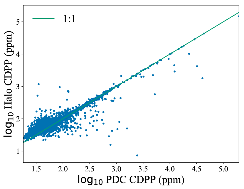
Figure 5: Correlation diagram of the lightkurve-computed 6.5 hr CDPP for K2 Campaign 6 stars in the magnitude range $11.5<Kp<12.5$, as processed with the PDC pipeline ($x$-axis) and TV-min pipeline ($y$-axis), both after correction and whitening with k2sc. The severe outliers where halo significantly outperforms PDC are shown by individual inspection to consist of stars for which there is contamination, or for which the SAP aperture assigned by the Kepler pipeline is significantly smaller than the PSF.

Histograms of the CDPPs of the SAP, PDC and halo light curves with and without k2sc are displayed in Figure 6. We see that both halo and PDC significantly outperform SAP, with halo performing better than PDC with no additional correction. Nevertheless, after k2sc, we found that the best PDC light curves have a smaller CDPP than the best similarly pointing-corrected halo. We conjecture that PDC with its improved calibration for common-mode systematics and blended/background light is correcting for effects that halo, as a single-star and instrument-agnostic method, does not.

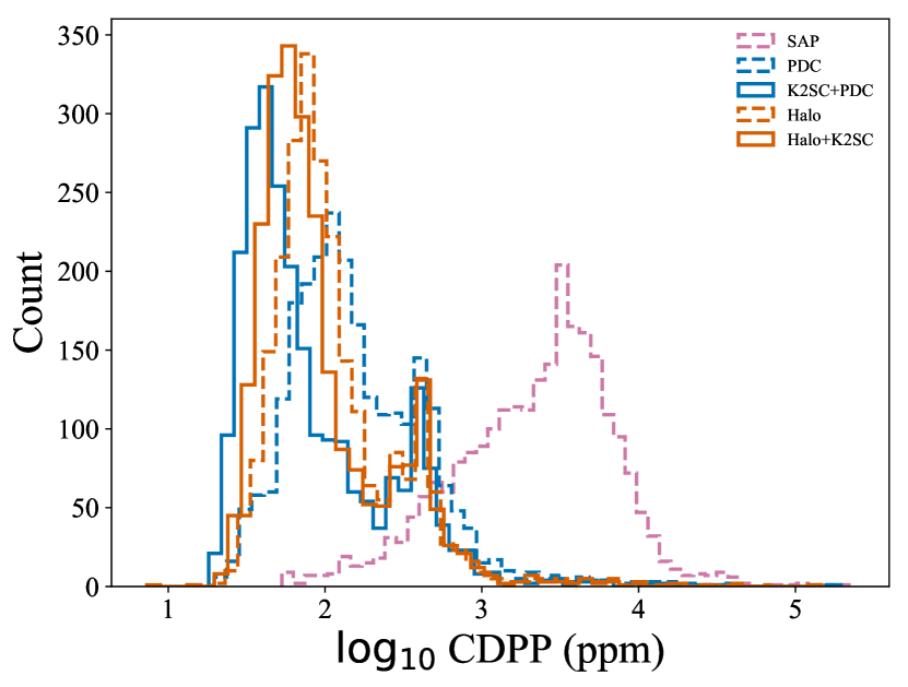
Figure 6: Histograms of the lightkurve-computed 6.5 hr CDPP for five different pipelines applied to K2 Campaign 6 stars in the magnitude range $11.5<Kp<12.5$: SAP (purple dashed), PDC with (blue solid) and without (blue dashed) k2sc, and TV-min with (orange solid) and without (orange dashed) k2sc.

3 Sample

The full sample of the 161 stars for which halo apertures were obtained is listed in Table The K2 Bright Star Survey I: Methodology and Data Release. A $B$, $V$ color-magnitude diagram is displayed in Figure 7, omitting the very-red carbon star HR 3541, whose $B-V$ color is 3.23. Following the successful pilot observations of the Pleiades B stars in Campaign 4, we proposed halo photometry through dedicated K2 Guest Observer Programs from Campaign 6 onwards. Target selection was performed by cross-matching Hipparcos (van Leeuwen, 2007) with the K2 Ecliptic Plane Input Catalog (EPIC, Huber et al., 2016) and selecting all targets on silicon brighter than $Kp<6$ on silicon. M giants which pulsate with periods that are long compared to a K2 campaign were removed. We requested short-cadence observations for a small number of unevolved stars for which the expected timescales of oscillations cannot be sufficiently sampled with long-cadence data, such as for $\delta$ Sct stars whose maximum frequencies can exceed the long-cadence Nyquist limit.

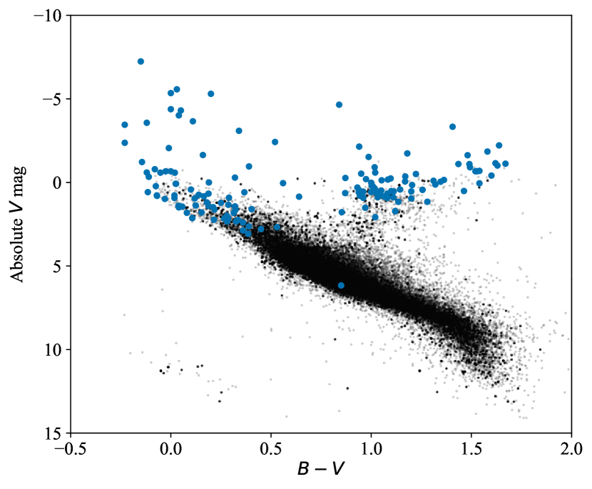
Figure 7: $B$, $V$ color-magnitude diagram of the halo sample overlaid on a random subset of K2 stars with high-SNR Gaia cross-matches, from the gaia-kepler.fun sample, with $B$ and $V$ magnitudes drawn from the EPIC catalog (Huber et al., 2016). We omit the very-red carbon star HR 3541, whose $B-V$ color is 3.23. The halo sample is seen to be more intrinsically luminous than K2 stars overall, and includes the most intrinsically luminous star observed by K2, $\rho$ Leonis. An interactive version of this plot is available at benjaminpope.github.io/data/cmd_halo.html.

Some very bright stars were observed with conventional apertures as part of these programs, but we exclude them from the present discussion and data release, which is oriented towards targets only observable with halo photometry. We include $\alpha$ Vir (Spica) and 69 Vir, which were observed in Campaign 6 without a halo aperture (in Campaign 17 Spica was re-observed, with a halo aperture). In Campaign 6 they were assigned normal apertures due an erroneous estimate of their Kepler magnitudes and simple aperture photometry performed extremely poorly, so we have processed these data with the halo pipeline. The stars in Campaign 18 in our sample were also on-silicon in Campaign 5, but were not assigned apertures suitable for halo photometry in C5. A possible further extension of the present work would be to recover C5 light curves for these objects using smear and/or modified halo photometry.

Seven stars in Campaign 13 and one in Campaign 16 were assigned short-cadence halo apertures. For these targets we have provided both long- and short-cadence reductions. Following the analysis in Section 2 showing the insensitivity of short-cadence CDPP to lags longer than $\sim 100$ cad and to $k\in{1,2}$, and for consistency with long cadence, we have adopted a 300 epoch lag (i.e. $30\times$ the long-cadence lag of 10) and the L1 TV objective function. With their many time samples, the short-cadence stars are computationally intractable for the Gaussian Process model in k2sc and we present otherwise uncalibrated halo light curves.

Analyses for some of our sample have been previously published, we include their light curves in this data release: the Pleiades’ Seven Sisters (White et al., 2017), $\alpha$ Tau (Aldebaran; Farr et al., 2018), $\iota$ Lib (Buysschaert et al., 2018), and $\epsilon$ Tau (Ain; Arentoft et al., 2019), as well as $\rho$ Leo, which was studied with halo pixels but without our objective functions (Aerts et al., 2018).

4 Discussion

4.1 Comparison with ‘Raw’ Halo

The blue supergiant $\rho$ Leonis, observed in Campaign 14, was studied with halo photometry but without the TV-min method by Aerts et al. (2018). In that reduction, Aerts et al. (2018) used four different aperture masks to extract raw light curves, and detrended these for K2 systematics with k2sc and a polynomial to account for long-term drift. They detected photometric variability at the star’s rotation period of 26.8 d and also multiperiodic low-frequency variability ($<1.5\text{d}^{-1}$). The k2sc systematics and variability models, residuals, halo apertures, and periodograms are shown in Figure 3, and a comparison with the Aerts et al. (2018) lightcurve in Figure 8. There is excellent agreement between the light curves produced by both methods. It is easiest to compare the methods in the power-spectral domain, where we see a reduction of only a few percent in the amplitude of oscillations in the TV-min and the Aerts et al. (2018) lightcurve; at high frequencies, both methods show significant residual systematics at the K2 thruster-firing frequencies, but the TV-min lightcurve shows a lower white noise floor by a factor of $\sim 3$.

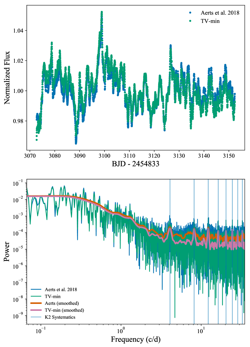
Figure 8: Top: halo light curves of $\rho$ Leonis from Aerts et al. (2018) (blue) and TV-min from the present paper (green). Bottom: Lomb-Scargle power spectral densities of the Aerts (blue) and TV-min (green) observations, with smoothed power spectral densities overplotted in orange and purple respectively and the K2 thruster firing frequencies highlighted with pale blue vertical lines. There is excellent agreement between the light curves and power spectra at high frequencies, with some residual thruster firing systematics in both light curves, and a factor of $\sim 3$ lower white noise floor in the TV-min power spectrum.

4.2 Oscillating Red Giants

Thirty-one of the red giants in our sample have detectable stochastically-excited solar-like acoustic (p-mode) oscillations. In the asymptotic limit, these consist of a comb of modes separated by the large frequency separation $\Delta\nu$, approximately the sound-crossing-time of the star, with a Gaussian envelope centred on the frequency of maximum power $\nu_{\rm max}$, which scales with the acoustic cutoff frequency at the star’s surface. These $\Delta\nu$ and $\nu_{\rm max}$ values can be used to constrain stellar fundamental parameters, such as radius, mass, and age (e.g. Hekker & Christensen-Dalsgaard, 2017, for a recent review). Detailed studies of the deviations from the asymptotic limit for p-modes, e.g. due to acoustic ‘glitches’, provide information on the He content and mixing processes at the bottom of the convective envelope (e.g. Verma et al., 2019). On the other hand, dipole mixed modes, which have a g-mode character in the inner regions of the star, fulfill an asymptotic period spacing determined by the buoyancy frequency inside the star. This spacing can be used to accurately determine the stellar evolutionary stage, and allows us to distinguish between hydrogen shell and core helium burning (Bedding et al., 2011). Summary plots for a good example of such a star, $\eta$ Cancri, are shown in Figure 9.

Using the Sydney pipeline (Huber et al., 2009) with modifications to the extraction of $\Delta\nu$ detailed in Yu et al. (2018), we extract the global asteroseismic parameters $\nu_{\rm max}$ and $\Delta\nu$ for the 31 red giants for which oscillations are detected with sufficient signal-to-noise. These parameters are listed in Table 2; the stars are noted as showing ‘RG’ variability in Table The K2 Bright Star Survey I: Methodology and Data Release, whereas this field is left blank for stars of luminosity class III for which oscillations are not unambiguously detected. High precision spectroscopy of these stars would permit detailed stellar modelling and the extraction of precise elemental abundances, which would make these stars useful as benchmarks for large spectroscopic surveys or testing detailed stellar models. This sample will be an addition to the 36 Gaia FGK benchmark stars (Jofré et al., 2014; Heiter et al., 2015; Jofré et al., 2018), the 23 BRITE-Constellation asteroseismic red giants (Kallinger et al., 2019), and the 33 Kepler Smear Campaign spectroscopic benchmark red giants (Pope et al., 2019).

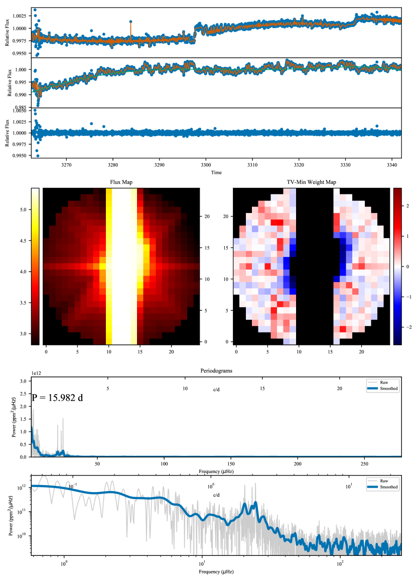
Figure 9: Summary plots for k2sc-corrected final halo light curve for the red giant $\eta$ Cancri, in the same format as Figure 3. Solar like oscillations are clearly detected with $\mbox{$\nu_{\rm max}$}=22.9\pm 0.9$ $\mu$Hz and $\mbox{$\Delta\nu$}=2.7\pm 0.03$ $\mu$Hz.

4.3 Eclipsing Binaries

We have detected two eclipsing binaries in our sample: the previously-known EB HR 6773 and the new detection 98 Tau. After subtracting an EB model for HR 6773, we find additional variability consistent with SPB pulsations.

The chemically-peculiar A0V star 98 Tau is of special interest for studies of surface inhomogeneity. We detected variability with a fundamental period of 1.74 d with twice as much power at the first harmonic ($P=0.87$ d), which is consistent with $\alpha^{2}$ CVn chemical spot modulation from a rapidly-rotating star. This star also experiences a V-shaped transit of fractional depth 0.16, which for a 1.87 $\mathrm{R}_{\sun}$ typical A0V star implies a grazing eclipse by a stellar mass companion. There are an unusually high number of background stars in the same photometric aperture as 98 Tau, and these were not all detected by deathstar and significantly contaminated the resulting lightcurve. As a result it was necessary to manually flag these objects using the ‘interact’ mode of lightkurve, as displayed in Figure 10. The eclipse is deep enough to be seen by eye in the diffuse light of 98 Tau using this interactive display, and is not associated with any of the background stars.

These systems contain variable stars in the brightest EBs in K2 , and are therefore unique targets for follow-up with smaller telescopes. With an eclipse to break degeneracies, models such as starry (Luger et al., 2019) has been shown to robustly and uniquely infer surface brightness maps from light curves. High-time-cadence photometry during transit, such as with CHEOPS (Broeg et al., 2013), will reveal the spatial distribution of the star’s chemical peculiarity or pulsation.

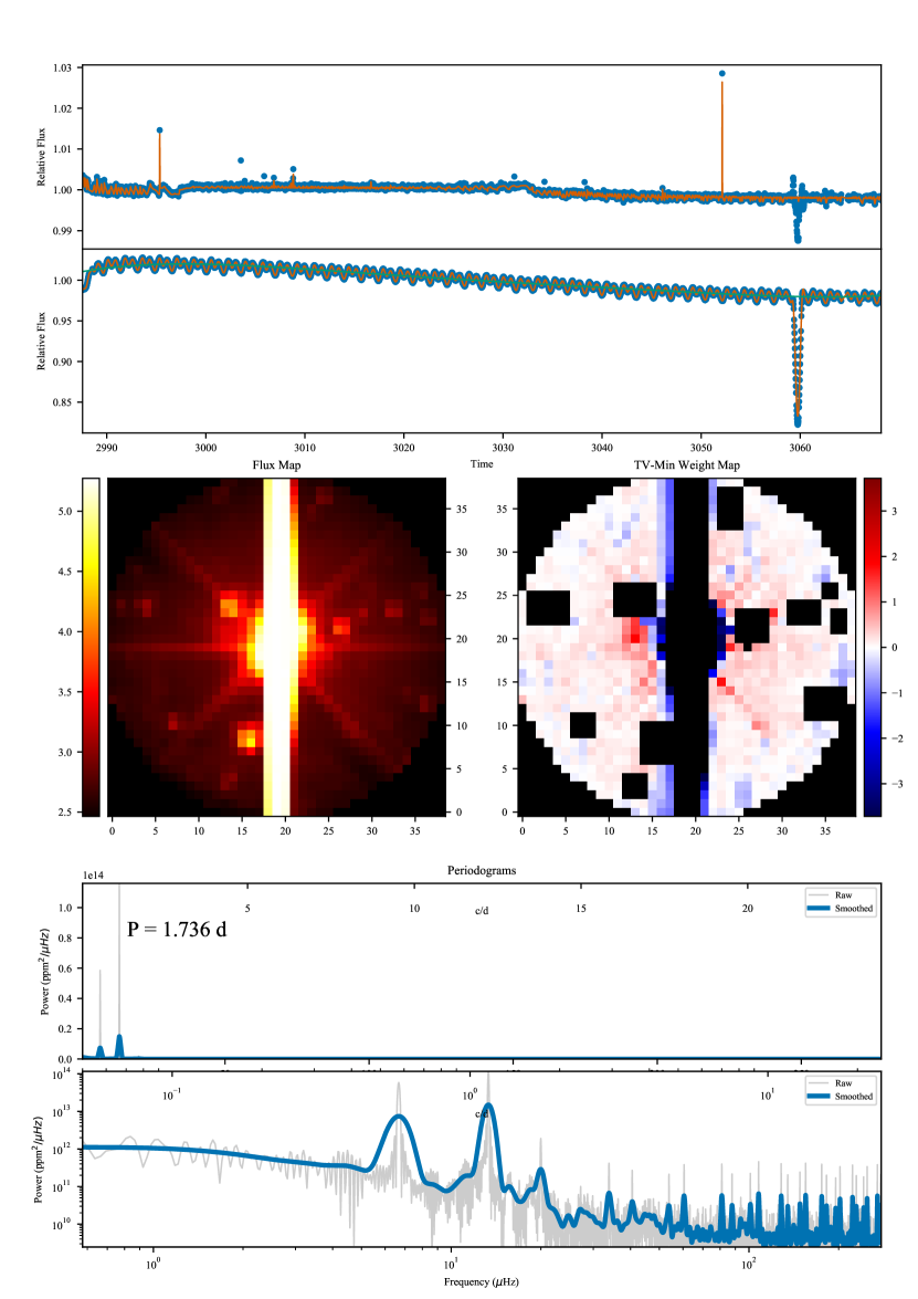
Figure 10: Summary plots for k2sc-corrected final halo light curve for the eclipsing binary 98 Tauri, in a similar format to Figure 3. Blacked-out pixels in the halo weights are background stars which were manually set to zero weight by hand. The residuals to the position and time GP are not shown, as the time GP fits poorly to the deep eclipse, though this did not adversely affect the pointing systematics model. The polynomial trend and Lomb-Scargle periodograms are conditioned on the out-of-transit points only.

4.4 Other Variables

Our dataset includes a rich variety of classical pulsators. We visually inspected the light curves and amplitude spectra to classify all non red-giant stars into traditional variability classes. We identify 23 stars showing $\delta$ Scuti pulsations and 20 with $\gamma$ Doradus pulsations, including 9 with hybrid $\delta$ Sct/$\gamma$ Dor variability; 14 slowly pulsating B stars (SPB stars), 3 $\beta$ Cephei pulsators, and 3 Cepheids; as well as 3 O stars and 5 blue supergiants showing low-frequency variability (as in Aerts et al., 2018; Bowman et al., 2019). In addition to this, the light curves of eight stars reveal rotational modulation, of which two have the characteristics of $\alpha^{2}$ CVn chemical spot modulation. The classes we have determined for each star are listed in Table The K2 Bright Star Survey I: Methodology and Data Release. A detailed frequency analysis of the variability in each star will be presented in a forthcoming paper.

5 Data Release and Open Science

The software halophot that implements halo photometry as described in this paper is available under a GPLv3 license from github.com/hvidy/halophot.

All light curves presented in this paper are available as High-Level Science Products from the Mikulski Archive for Space Telescopes (MAST). They are also available, together with the source code that produced the survey sample and this manuscript, from github.com/benjaminpope/k2halo.

6 Conclusions

We have presented an updated method for halo photometry, and used this to obtain light curves of 161 stars in K2 that were too saturated to be otherwise retrievable. These ubiquitously show variability, and we have presented global asteroseismic analysis of 31 red giants and variability classifications for all stars. This is a unique legacy sample for K2 , dramatically increasing the number of very bright stars that have been characterized with high-precision, rapid-time-cadence space photometry. We hope that our data release will be used for a variety of astrophysical investigations.

Some of the objects presented here are the subject of more detailed work in preparation, namely $\alpha$ Vir (Spica), interferometry and asteroseismology of the Hyades giants, and main-sequence stars with self-driven nonradial modes.

The sample of K2 bright stars presented here only includes those with halo apertures. While some others are available conventionally, many were not assigned target pixels and were not downloaded at all. Smear photometry has been used to recover the brightest otherwise-unobserved stars in nominal Kepler (Pope et al., 2019), and this can also be done in K2, although the sample is much smaller due to allocation of halo apertures and the systematics correction is more challenging. A natural extension of both pieces of work would be to produce smear light curves of all bright stars without halo apertures in K2, which would finally make the Kepler extended mission magnitude-complete at the bright end.

The halo method naturally extends to other contexts where simple aperture photometry is not possible, such as for saturated stars observed by the Transiting Exoplanet Survey Satellite (TESS; Ricker et al., 2015). Although the saturation limit is brighter ($T_{mag}\sim 6$) and this problem accordingly affects fewer stars and less badly, there are stars such as $\alpha$ Centauri and $\beta$ Hydri where the bleed column reaches the edge of the chip and a SAP light curve is irrecoverable. We expect that TV-min halo photometry will therefore be important in ensuring that TESS can observe the very brightest stars.

There are directions for improvement of the halo method itself, and for applying it beyond Kepler /K2 and TESS. It remains to be seen how well the method of optimizing convex objective functions can deal with significantly varying PSFs, such as from ground-based observations. The rapidly varying and moving seeing-limited PSF couples to flat field errors as is the case with Kepler , and leads to severe short-timescale instrumental noise. Self-calibration by the halo method, or a similar method, may permit improvements in ground-based photometry. Likewise, there may be other convex objective functions, including linear combinations of currently-used objective functions, which offer superior performance, for example by using combinations of different lagged functions to suppress systematics occurring at different timescales. The remaining unexplored space of convex objective functions may offer significant improvements on existing self-calibration techniques in high-cadence photometry and related problems in astronomy.

Table 1: All stars observed with halo photometry in K2.

Name	EPIC	Spectral	V	Campaign	Notes	Class
		Type	(mag)
$\eta$ Tau	200007767	B7III	2.986	4		SPB
27 Tau	200007768		3.763	4		SPB
17 Tau	200007769	B6IIIe	3.851	4		SPB
23 Tau	200007770	B6IVe	4.305	4		SPB
20 Tau	200007771	B8III	4.305	4		$\alpha^{2}\,\text{CVn}$
19 Tau	200007772	B6IV	4.448	4		SPB
28 Tau	200007773	B8Ve	5.192	4		SPB
$\gamma$ Tau	200007765	G9.5III	3.474	4		RG
$\delta^{1}$ Tau	200007766	G9.5III	3.585	4		RG
$\alpha$ Vir	212573842	B1V	0.97	6, 17	Normal Mask	SPB
69 Vir	212356048	K0III	4.75	6		–
$\zeta$ Sgr	200062593	A2.5V	2.585	7		$\gamma\,\text{Dor}$
$\pi$ Sgr	200062592	F2II-III	2.88	7		Supergiant
$\tau$ Sgr	200062591	K1.5III	3.31	7		RG
$\xi^{2}$ Sgr	200062590	G8/K0II/III	3.51	7		RG
$o$ Sgr	200062589	G9III	3.77	7		RG
52 Sgr	200062585	B8/9V	4.598	7		SPB + Rotation
$\nu^{1}$ Sgr	200062588	K1II	4.845	7		–
$\psi$ Sgr	200062584	K0/1III	4.85	7		–
43 Sgr	200062587	G8II-III	4.878	7		–
$\nu^{2}$ Sgr	200062586	K3-II-III	4.98	7		RG
$\epsilon$ Psc	200068392	G9IIIe	4.28	8		RG
$\zeta$ Psc A	200068393	A7IV	5.187	8		$\delta\,\text{Sct}$/$\gamma\,\text{Dor}$
80 Psc	200068394	F2V	5.5	8		$\gamma\,\text{Dor}$
42 Cet	200068399	G8IV	5.87	8		?
33 Cet	200068395	K4/5III	5.942	8		–
60 Psc	200068396	G8III	5.961	8		–
73 Psc	200068397	K5III	6.007	8		–
WW Psc	200068398	M2.5III	6.14	8		–
HR 243	200068400	G8/K0II/III	6.368	8		–
HR 161	200068401	K3III	6.407	8		–
HR 6766	200069361	G7:III	4.56	9		RG
HR 6842	200069360	K3II	4.627	9		–
4 Sgr	200069357	A0	4.724	9		–
11 Sgr	200069358	K0III	4.98	9		RG
7 Sgr	200069362	F2II-III	5.34	9		RG
15 Sgr	200069359	O9.7I	5.37	9		O
HR 6838	200069363	K2III	5.75	9		–
Y Sgr	200069364	F8II	5.75	9		Cepheid
HR 6716	200069365	B0I	5.77	9		SPB
HR 6681	200069366	A0V	5.929	9		–
9 Sgr	200069368	O4V	5.97	9		Supergiant
16 Sgr	200069367	O9.5III	6.02	9		RG
HR 6825	200069369	ApSip	6.15	9		$\gamma\,\text{Dor}$
63 Oph	200069370	O8II	6.2	9		O
HR 6679	200069373	A1V	6.469	9		–
HD 165784	200069371	A2I	6.58	9		–
HD 161083	200069374	F0V	6.58	9		$\delta\,\text{Sct}$/$\gamma\,\text{Dor}$
5 Sgr	200069372	K0III	6.64	9		RG
HD 167576	200069378	K1III	6.66	9		–
HR 6773	200069380	B3/5IV	6.71	9		EB + SPB
HD 163296	200071159	A1Vpe	6.85	9		$\gamma\,\text{Dor}$
HD 165052	200069379	O6V+O8V	6.87	9		O
17 Sgr	200069375	G8/K0III	6.886	9		–
HD 169966	200069376	G8/K0III	6.97	9		–
HD 162030	200069377	K1III	7.02	9		–
$\gamma$ Vir	200084004	F1V+F2Vm	2.74	10		$\gamma\,\text{Dor}$
$\eta$ Vir	200084005	A2IV	3.9	10		$\delta\,\text{Sct}$
21 Vir	200084006	B9V	5.48	10		–
FW Vir	200084007	M3+IIICa0.5	5.71	10		–
HR 4837	200084008	G8III	5.918	10		–
HR 4591	200084009	K1III	6.316	10		–
HR 4613	200084010	G8/K0III	6.364	10		–
HD 107794	200084011	K0III	6.46	10		–
$\theta$ Oph	200128906	OB	3.26	11		$\beta$ Cep
44 Oph	200128907	A3m	4.153	11		–
45 Oph	200128908	F5III-IV	4.269	11		–
51 Oph	200128909	A0V	4.81	11		Rotation
36 Oph	200129035	K2V+K1V	5.03	11		Rotation
$o$ Oph	200128910		5.2	11		?
26 Oph	200129034	F3V	5.731	11		$\gamma\,\text{Dor}$
HR 6472	200128911	K0III	5.83	11		–
HR 6366	200128913	Fm	5.911	11		–
HR 6365	200128912	K0III	5.977	11		–
191 Oph	200128914	K0III	6.171	11		RG
$\kappa$ Psc	200164167	A2Vp	4.94	12		Rotation + $\delta\,\text{Sct}$
83 Aqr	200164168	F0V	5.47	12		$\delta\,\text{Sct}$/$\gamma\,\text{Dor}$
24 Psc	200164169	K0II/III	5.94	12		–
HR 8759	200164170	G5II/III	5.933	12		RG
14 Psc	200164171	A2II	5.87	12		Supergiant
HR 8921	200164172	K4/5III	6.191	12		–
81 Aqr	200164173	K4III	6.215	12		RG
HR 8897	200164174	K4III	6.34	12		–
$\alpha$ Tau	200173843	K5+III	0.86	13		–
$\theta^{2}$ Tau	200173845	A7III	3.41	13	SC	$\delta\,\text{Sct}$
$\epsilon$ Tau	200173844	G9.5III	3.53	13		RG
$\theta^{1}$ Tau	200173846	G9IIIe	3.84	13		f
$\kappa^{1}$ Tau	200173847	A7IV	4.201	13	SC	$\delta\,\text{Sct}$
$\delta^{3}$ Tau	200173849	A2IV	4.25	13	C4	Supergiant
$\tau$ Tau	200173850	B3V	4.258	13		SPB
$\upsilon$ Tau	200173848	A8V	4.282	13	SC	$\delta\,\text{Sct}$
$\rho$ Tau	200173851	A8V	4.65	13	SC	$\delta\,\text{Sct}$
11 Ori	200173853	A1Vp	4.661	13		Rotation
HR 1427	200173855	A6IV	4.764	13	SC	$\gamma\,\text{Dor}$?
15 Ori	200173854	F2IV	4.82	13		$\gamma\,\text{Dor}$
75 Tau	200173852	K1III	4.969	13		RG
97 Tau	200173857	A7IV	5.085	13	SC	$\delta\,\text{Sct}$/$\gamma\,\text{Dor}$
HR 1684	200173856	K5III	5.163	13		–
$\kappa^{2}$ Tau	200173859	F0V	5.264	13	SC	$\delta\,\text{Sct}$/$\gamma\,\text{Dor}$
56 Tau	200173861	A0Vp	5.346	13		$\delta\,\text{Sct}$
81 Tau	200173860	Am	5.454	13		–
53 Tau	200173864	B9Vp	5.482	13		SPB
HR 1585	200173858	K1III	5.49	13		RG
80 Tau	200173866	F0V	5.552	13		$\gamma\,\text{Dor}$
51 Tau	200173865	F0V	5.631	13		$\delta\,\text{Sct}$
HR 1403	200173867	Am	5.711	13		–
89 Tau	200173868	F0V	5.776	13		$\delta\,\text{Sct}$/$\gamma\,\text{Dor}$
HR 1576	200173871	B9V	5.776	13		SPB
98 Tau	200173870	A0V	5.785	13		EB + $\alpha^{2}\,\text{CVn}$
99 Tau	200173862	K0III	5.806	13		RG
105 Tau	200173869	B2Ve	5.92	13		$\beta$ Cep
HR 1554	200173874	F2IV	5.961	13		$\delta\,\text{Sct}$/$\gamma\,\text{Dor}$
HR 1385	200173875	F4V	5.965	13	C4	$\delta\,\text{Sct}$/$\gamma\,\text{Dor}$
HR 1741	200173873	K0III	6.107	13		–
HR 1633	200173872	K0	6.188	13		RG
HR 1755	200173876	K0III	6.205	13		RG
$\rho$ Leo	200182931	B1I	3.87	14		Supergiant
58 Leo	200182925	K0.5IIIe	4.838	14		RG
48 Leo	200182926	G8.5IIIe	5.07	14		RG
53 Leo	200182928	A2V	5.312	14		$\delta\,\text{Sct}$
65 Leo	200182927	K0III	5.52	14		RG
35 Sex	200182929	K1+K2III	5.79	14		RG
43 Leo	200182930	K3III	6.08	14		RG
$\delta$ Sco	200194910	B0.3IV	2.32	15		$\beta$ Cep
$\gamma$ Lib	200194911	G8.5III	3.91	15		RG
$\iota^{1}$ Lib	200194912	B9IVp	4.54	15		Rotation + SPB
41 Lib	200194913	G8III/IV	5.359	15		RG
$\zeta^{4}$ Lib	200194914	B3V	5.499	15		$\beta$ Cep
HR 5762	200194915	A2IV	5.52	15		–
HR 5806	200194916	K0III	5.79	15		RG
$\zeta^{3}$ Lib	200194917	K0III	5.806	15		RG
HR 5810	200194918	K0III	5.816	15		RG
$\iota^{2}$ Lib	200194919	A2V	6.066	15		$\delta\,\text{Sct}$
HR 5620	200194920	K0III	6.14	15		RG
28 Lib	200194921	G8II/III	6.17	15		RG
HD 138810	200194958	K1III	7.02	15		–
$\delta$ Cnc	200200356	K0+IIIb	3.94	16		–
$\alpha$ Cnc	200200357	A5m	4.249	16		Rotation
$\xi$ Cnc	200200358	G8.5IIIe	5.149	16		–
$o^{1}$ Cnc	200200360	A5III	5.22	16		–
$\eta$ Cnc	200200359	K3III	5.325	16, 18		RG
45 Cnc	200200728	A3III+G7III	5.65	16	SC	$\delta\,\text{Sct}$
$o^{2}$ Cnc	200200361	F0IV	5.677	16		–
50 Cnc	200200363	A1Vp	5.885	16, 18		$\delta\,\text{Sct}$
82 Vir	200213053	M1+III	5.01	17		–
76 Vir	200213054	G8III	5.21	17		RG
68 Vir	200213055	K5III	5.25	17		–
80 Vir	200213056	K0III	5.706	17		RG
HR 5106	200213057	A0V	5.932	17		$\delta\,\text{Sct}$
HR 5059	200213058	A8V	5.965	17		$\gamma\,\text{Dor}$
$\gamma$ Cnc	200233186	A1IV	4.652	18	C5	–
$\zeta$ Cnc	200233643	F8V+G0V	4.67	18	C5	–
60 Cnc	200233188	K5III	5.44	18	C5, C16	–
49 Cnc	200233189	A1Vp	5.66	18	C5	Rotation + $\gamma\,\text{Dor}$
HR 3264	200233190	K1III	5.798	18	C5	RG
29 Cnc	200233192	A5V	5.948	18	C5	$\delta\,\text{Sct}$/$\gamma\,\text{Dor}$
HR 3222	200233193	G8III	6.047	18	C5	–
21 Cnc	200233196	M2III	6.08	18	C5	–
25 Cnc	200233644	F5IIIm?	6.1	18	C5	–
HR 3558	200233195	K1III	6.146	18	C5	–
HR 3541	200233194	C-N4.5	6.4	18	C5	–

References. — ^a: White et al. (2017); ^b: Buysschaert et al. (2018); ^c: Farr et al. (2018); ^d: Arentoft et al. (2019); ^e: Aerts et al. (2018); ^f: Light curve shows RG pulsations, but is also significantly contaminated by the higher amplitude $\delta$ Sct pulsations of the nearby $\theta^{2}$ Tau.

Note. — Some targets are known by proper names. $\eta$ Tau: Alcyone; 27 Tau: Atlas; 17 Tau: Electra; 20 Tau: Maia; 23 Tau: Merope; 19 Tau: Taygeta; 28 Tau: Pleione; $\zeta$ Sgr: Ascella; $\pi$ Sgr: Albaldah; $\nu^{1}$ Sgr: Ainalrami; $\zeta$ Psc A: Revati; $\gamma$ Vir: Porrima; $\eta$ Vir: Zaniah; $\alpha$ Tau: Aldebaran; $\delta$ Sco: Dschubba; $\gamma$ Lib: Zubenelhakrabi; $\delta$ Cnc: Asellus Australis; $\alpha$ Cnc: Acubens; $\alpha$ Vir: Spica; 36 Oph: Guniibuu; $\gamma$ Tau: Prima Hyadum; $\delta^{1}$ Tau: Secunda Hyadum; $\theta^{2}$ Tau: Chamukuy; $\epsilon$ Tau: Ain; $\xi$ Cnc: Nahn; $\gamma$ Cnc: Asellus Borealis; $\zeta$ Cnc: Tegmine

Table 2: Global asteroseismic parameters for the 31 red giants for which solar-like oscillations were detected.

Name	EPIC	$\nu_{\rm max}$	$\Delta\nu$
		($\mu$Hz)	($\mu$Hz)
$\gamma$ Tau	200007765	62.89 $\pm$ 1.44	5.56 $\pm$ 0.17
$\delta^{1}$ Tau	200007766	62.59 $\pm$ 1.74	5.72 $\pm$ 0.07
$\nu^{2}$ Sgr	200062586	7.29 $\pm$ 0.15	1.31 $\pm$ 0.05
$o$ Sgr	200062589	46.28 $\pm$ 1.02	4.82 $\pm$ 0.06
$\xi^{2}$ Sgr	200062590	11.71 $\pm$ 0.65	1.87 $\pm$ 0.15
$\tau$ Sgr	200062591	19.85 $\pm$ 0.80	2.46 $\pm$ 0.07
$\pi$ Sgr	200062592	46.95 $\pm$ 0.43	5.97 $\pm$ 0.20
$\epsilon$ Psc	200068392	33.31 $\pm$ 1.22	3.62 $\pm$ 0.07
11 Sgr	200069358	38.03 $\pm$ 0.84	4.01 $\pm$ 0.13
HR 6766	200069361	20.60 $\pm$ 4.19	2.42 $\pm$ 0.41
7 Sgr	200069362	13.59 $\pm$ 0.97	1.98 $\pm$ 0.20
HR 6716	200069365	10.68 $\pm$ 3.38	1.77 $\pm$ 0.28
16 Sgr	200069367	13.76 $\pm$ 0.34	2.23 $\pm$ 0.11
5 Sgr	200069372	47.78 $\pm$ 0.95	4.65 $\pm$ 0.05
191 Oph	200128914	29.19 $\pm$ 0.92	3.91 $\pm$ 0.10
HR 8759	200164170	10.14 $\pm$ 0.39	1.56 $\pm$ 0.05
81 Aqr	200164173	11.38 $\pm$ 0.23	1.69 $\pm$ 0.06
$\epsilon$ Tau	200173844	54.46 $\pm$ 1.44	5.13 $\pm$ 0.13
75 Tau	200173852	34.95 $\pm$ 0.96	4.15 $\pm$ 0.04
HR 1585	200173858	9.38 $\pm$ 1.01	1.48 $\pm$ 0.10
99 Tau	200173862	21.44 $\pm$ 1.07	2.41 $\pm$ 0.07
HR 1755	200173876	18.78 $\pm$ 0.41	2.04 $\pm$ 0.04
58 Leo	200182925	17.01 $\pm$ 0.46	1.97 $\pm$ 0.23
48 Leo	200182926	53.32 $\pm$ 0.79	5.43 $\pm$ 0.04
65 Leo	200182927	61.65 $\pm$ 1.38	6.43 $\pm$ 0.03
35 Sex	200182929	11.52 $\pm$ 0.15	1.52 $\pm$ 0.05
43 Leo	200182930	71.61 $\pm$ 2.81	7.20 $\pm$ 0.08
$\gamma$ Lib	200194911	34.89 $\pm$ 0.98	3.57 $\pm$ 0.10
41 Lib	200194913	54.25 $\pm$ 1.79	5.19 $\pm$ 0.03
HR 5806	200194916	53.22 $\pm$ 0.75	4.91 $\pm$ 0.06
$\zeta^{3}$ Lib	200194917	44.18 $\pm$ 1.00	3.55 $\pm$ 0.26
HR 5810	200194918	45.02 $\pm$ 0.46	4.46 $\pm$ 0.03
HR 5620	200194920	96.84 $\pm$ 0.74	9.28 $\pm$ 0.03
28 Lib	200194921	41.05 $\pm$ 0.86	4.10 $\pm$ 0.17
$\eta$ Cnc	200200359	22.91 $\pm$ 0.86	2.65 $\pm$ 0.03
76 Vir	200213054	40.02 $\pm$ 2.62	3.76 $\pm$ 0.09
80 Vir	200213056	36.98 $\pm$ 1.83	4.38 $\pm$ 0.08
HR 3264	200233190	22.93 $\pm$ 0.17	3.00 $\pm$ 0.18

References

- Aerts et al. (2018) Aerts, C., Bowman, D. M., Símon-Díaz, S., et al. 2018, MNRAS, 476, 1234, doi: 10.1093/mnras/sty308
- Aigrain et al. (2015) Aigrain, S., Hodgkin, S. T., Irwin, M. J., Lewis, J. R., & Roberts, S. J. 2015, MNRAS, 447, 2880, doi: 10.1093/mnras/stu2638
- Aigrain et al. (2016) Aigrain, S., Parviainen, H., & Pope, B. J. S. 2016, MNRAS, 459, 2408, doi: 10.1093/mnras/stw706
- Akeson et al. (2013) Akeson, R. L., Chen, X., Ciardi, D., et al. 2013, PASP, 125, 989, doi: 10.1086/672273
- Arentoft et al. (2019) Arentoft, T., Grundahl, F., White, T. R., et al. 2019, A&A, 622, A190, doi: 10.1051/0004-6361/201834690
- Astropy Collaboration et al. (2013) Astropy Collaboration, Robitaille, T. P., Tollerud, E. J., et al. 2013, A&A, 558, A33, doi: 10.1051/0004-6361/201322068
- Bedding et al. (2011) Bedding, T. R., Mosser, B., Huber, D., et al. 2011, Nature, 471, 608, doi: 10.1038/nature09935
- Borucki et al. (2010) Borucki, W. J., Koch, D., Basri, G., et al. 2010, Science, 327, 977, doi: 10.1126/science.1185402
- Bowman et al. (2019) Bowman, D. M., Burssens, S., Pedersen, M. G., et al. 2019, Nature Astronomy, doi: 10.1038/s41550-019-0768-1
- Broeg et al. (2013) Broeg, C., Fortier, A., Ehrenreich, D., et al. 2013, in European Physical Journal Web of Conferences, Vol. 47, European Physical Journal Web of Conferences, 03005
- Buysschaert et al. (2018) Buysschaert, B., Neiner, C., Aerts, C., White, T. R., & Pope, B. J. S. 2018, in SF2A-2018: Proceedings of the Annual meeting of the French Society of Astronomy and Astrophysics, 369–372
- Christiansen et al. (2012) Christiansen, J. L., Jenkins, J. M., Caldwell, D. A., et al. 2012, Publications of the Astronomical Society of the Pacific, 124, 1279, doi: 10.1086/668847
- Ester et al. (1996) Ester, M., Kriegel, H.-P., Sander, J., & Xu, X. 1996, in Proceedings of the Second International Conference on Knowledge Discovery and Data Mining, KDD’96 (AAAI Press), 226–231. http://dl.acm.org/citation.cfm?id=3001460.3001507
- Farr et al. (2018) Farr, W. M., Pope, B. J. S., Davies, G. R., et al. 2018, ApJ, 865, L20, doi: 10.3847/2041-8213/aadfde
- Gilliland et al. (2010) Gilliland, R. L., Jenkins, J. M., Borucki, W. J., et al. 2010, ApJ, 713, L160, doi: 10.1088/2041-8205/713/2/L160
- Guzik et al. (2016) Guzik, J. A., Houdek, G., Chaplin, W. J., et al. 2016, ApJ, 831, 17, doi: 10.3847/0004-637X/831/1/17
- Heiter et al. (2015) Heiter, U., Jofré, P., Gustafsson, B., et al. 2015, A&A, 582, A49, doi: 10.1051/0004-6361/201526319
- Hekker & Christensen-Dalsgaard (2017) Hekker, S., & Christensen-Dalsgaard, J. 2017, A&A Rev., 25, 1, doi: 10.1007/s00159-017-0101-x
- Howell et al. (2014) Howell, S. B., Sobeck, C., Haas, M., et al. 2014, PASP, 126, 398, doi: 10.1086/676406
- Huber et al. (2009) Huber, D., Stello, D., Bedding, T. R., et al. 2009, Communications in Asteroseismology, 160, 74. https://arxiv.org/abs/0910.2764
- Huber et al. (2016) Huber, D., Bryson, S. T., Haas, M. R., et al. 2016, ApJS, 224, 2, doi: 10.3847/0067-0049/224/1/2
- Jofré et al. (2018) Jofré, P., Heiter, U., Tucci Maia, M., et al. 2018, Research Notes of the American Astronomical Society, 2, 152, doi: 10.3847/2515-5172/aadc61
- Jofré et al. (2014) Jofré, P., Heiter, U., Soubiran, C., et al. 2014, A&A, 564, A133, doi: 10.1051/0004-6361/201322440
- Jones et al. (2001) Jones, E., Oliphant, T., Peterson, P., & Others. 2001, SciPy: Open source scientific tools for Python. http://www.scipy.org/
- Kallinger & Weiss (2018) Kallinger, T., & Weiss, W. W. 2018, in 3rd BRITE Science Conference, Vol. 8, 170–174
- Kallinger et al. (2019) Kallinger, T., Beck, P. G., Hekker, S., et al. 2019, A&A, 624, A35, doi: 10.1051/0004-6361/201834514
- Kolenberg et al. (2011) Kolenberg, K., Bryson, S., Szabó, R., et al. 2011, MNRAS, 411, 878, doi: 10.1111/j.1365-2966.2010.17728.x
- Lomb (1976) Lomb, N. R. 1976, Ap&SS, 39, 447, doi: 10.1007/BF00648343
- Luger et al. (2019) Luger, R., Agol, E., Foreman-Mackey, D., et al. 2019, AJ, 157, 64, doi: 10.3847/1538-3881/aae8e5
- Luger et al. (2018) Luger, R., Kruse, E., Foreman-Mackey, D., Agol, E., & Saunders, N. 2018, AJ, 156, 99, doi: 10.3847/1538-3881/aad230
- Lund et al. (2015) Lund, M. N., Handberg, R., Davies, G. R., Chaplin, W. J., & Jones, C. D. 2015, ApJ, 806, 30, doi: 10.1088/0004-637X/806/1/30
- Maclaurin et al. (2015) Maclaurin, D., Duvenaud, D., & Adams, R. P. 2015, in ICML 2015 AutoML Workshop
- Metcalfe et al. (2015) Metcalfe, T. S., Creevey, O. L., & Davies, G. R. 2015, ApJ, 811, L37, doi: 10.1088/2041-8205/811/2/L37
- Metcalfe et al. (2012) Metcalfe, T. S., Chaplin, W. J., Appourchaux, T., et al. 2012, ApJ, 748, L10, doi: 10.1088/2041-8205/748/1/L10
- Pablo et al. (2016) Pablo, H., Whittaker, G. N., Popowicz, A., et al. 2016, PASP, 128, 125001, doi: 10.1088/1538-3873/128/970/125001
- Parker et al. (2019) Parker, A. H., Hörst, S. M., Ryan, E. L., & Howett, C. J. A. 2019, arXiv e-prints. https://arxiv.org/abs/1906.04220
- Pérez & Granger (2007) Pérez, F., & Granger, B. E. 2007, Computing in Science and Engineering, 9, 21, doi: 10.1109/MCSE.2007.53
- Pope et al. (2016a) Pope, B. J. S., Parviainen, H., & Aigrain, S. 2016a, MNRAS, 461, 3399, doi: 10.1093/mnras/stw1373
- Pope et al. (2016b) Pope, B. J. S., White, T. R., Huber, D., et al. 2016b, MNRAS, 455, L36, doi: 10.1093/mnrasl/slv143
- Pope et al. (2019) Pope, B. J. S., Davies, G. R., Hawkins, K., et al. 2019, arXiv e-prints. https://arxiv.org/abs/1905.09831
- Ricker et al. (2015) Ricker, G. R., Winn, J. N., Vanderspek, R., et al. 2015, Journal of Astronomical Telescopes, Instruments, and Systems, 1, 014003, doi: 10.1117/1.JATIS.1.1.014003
- Scargle (1982) Scargle, J. D. 1982, ApJ, 263, 835, doi: 10.1086/160554
- Tkachenko et al. (2014) Tkachenko, A., Degroote, P., Aerts, C., et al. 2014, MNRAS, 438, 3093, doi: 10.1093/mnras/stt2421
- van Leeuwen (2007) van Leeuwen, F. 2007, A&A, 474, 653, doi: 10.1051/0004-6361:20078357
- Verma et al. (2019) Verma, K., Raodeo, K., Basu, S., et al. 2019, MNRAS, 483, 4678, doi: 10.1093/mnras/sty3374
- Vinícius et al. (2018) Vinícius, Z., Barentsen, G., Hedges, C., & Gully-Santiago, M. 2018, KeplerGO/lightkurve: 1.0.0.dev1: First development release of lightkurve, doi: 10.5281/zenodo.1181929. https://doi.org/10.5281/zenodo.1181929
- Walker et al. (2003) Walker, G., Matthews, J., Kuschnig, R., et al. 2003, PASP, 115, 1023, doi: 10.1086/377358
- Weiss et al. (2014) Weiss, W. W., Rucinski, S. M., Moffat, A. F. J., et al. 2014, PASP, 126, 573, doi: 10.1086/677236
- White et al. (2013) White, T. R., Huber, D., Maestro, V., et al. 2013, MNRAS, 433, 1262, doi: 10.1093/mnras/stt802
- White et al. (2017) White, T. R., Pope, B. J. S., Antoci, V., et al. 2017, MNRAS, 471, 2882, doi: 10.1093/mnras/stx1050
- Yu et al. (2018) Yu, J., Huber, D., Bedding, T. R., et al. 2018, ApJS, 236, 42, doi: 10.3847/1538-4365/aaaf74
- Zhu et al. (1999) Zhu, C., H. Byrd, R., & Lu, P. 1999