Benchmarking simplified template cross sections in $WH$ production

Abstract

Simplified template cross sections define a framework for the measurement and dissemination of kinematic information in Higgs measurements. We benchmark the currently proposed setup in an analysis of dimension-6 effective field theory operators for $WH$ production. Calculating the Fisher information allows us to quantify the sensitivity of this framework to new physics and study its dependence on phase space. New machine-learning techniques let us compare the simplified template cross section framework to the full, high-dimensional kinematic information. We show that the way in which we truncate the effective theory has a sizable impact on the definition of the optimal simplified template cross sections.

1 Introduction

Since the discovery of the Higgs boson at the LHC in 2012, the experimental and theoretical communities have focused intense scrutiny on the question of whether the observed particle has exactly the properties predicted by the Standard Model (SM) Dawson:2018dcd . The interpretation of the vast number of Higgs measurements requires a theoretical framework, which should be as flexible as possible. From a theoretical perspective and given that there are no non-SM particles observed at the electroweak scale, potential deviations from the SM are best analyzed in an effective field theory (EFT) approach Brivio:2017vri . Such a framework allows us to systematically include both rate information and kinematic distributions in the analysis Butter:2016cvz ; Brivio:2016fzo . In this study, we assume that the Higgs boson is in an $SU(2)_{L}$ doublet and work in the so-called Standard Model Effective Field Theory (SMEFT)  In this case deviations from the SM are parameterized in terms of a series of $SU(3)_{c}\times SU(2)_{L}\times U(1)_{Y}$ invariant operators and possible new physics effects are contained in the Wilson coefficients of these operators. The expansion involves a new high energy scale $\Lambda$, and we truncate the expansion with dimension-6 operators, whose effects are generically suppressed relative to SM predictions by factors of $v^{2}/\Lambda^{2}$ or $E^{2}/\Lambda^{2}$.

To interpret Higgs measurements in a combined experimental and theory analysis we need to a) develop an efficient strategy to extract the maximum information from Higgs events, and b) publish this information in an efficient form. Many analyses focus on total rate measurements, but the available global fits have shown that kinematic information on new Lorentz structures provides the most powerful limits on new physics, for instance, exploiting the boosted regime of $WH$ production Banerjee:2013apa ; Butter:2016cvz ; DiVita:2017vrr ; Ellis:2018gqa ; Almeida:2018cld ; Biekotter:2018rhp . For the first aspect this means that total or fiducial rate measurements alone are not useful. As for the second question, the experimental collaborations could choose to publish full likelihoods ATL-PHYS-PUB-2019-029 ; Collaboration:2242860 ; Cranmer:2013hia , which would ensure the most accurate modeling of systematic uncertainties and their correlations. However, despite some recent progress this strategy has not been widely adapted. Lacking the full likelihoods, the publication of measured event counts or cross sections in all bins of a histogram including uncertainties and their correlations is desirable Maguire:2017ypu . In reality, global fitting projects Leung:1984ni ; Buchmuller:1985jz ; GonzalezGarcia:1999fq ; Grojean:2018dqj ; deBlas:2016nqo ; Ellis:2018gqa often rely on extracting the necessary information from plots in publications and backwards-engineering as much of the analyses as possible.

An ad-hoc solution to these issues is the use of simplified template cross sections (STXS) Tackmann:2138079 ; Berger:2019wnu which propose to measure and publish cross sections in slices of simple phase-space parameters. They have been proposed for all major Higgs production channels and are continuously developed alongside the corresponding analysis opportunities. Given the established SMEFT approach we can benchmark any proposed method of extracting and publishing kinematic event information. A particularly well-suited approach for benchmarking is based on information geometry. Its central object, the Fisher information, encodes the maximal precision with which continuous parameters of a Lagrangian can be measured, and therefore allows us to directly compare the power of single LHC observables or STXS to the power of multivariate analysis strategies Brehmer:2016nyr ; Brehmer:2017lrt . In our case, these parameters are the Wilson coefficients of the dimension-6 SMEFT operators. Until now, a major limiting factor in this approach was that detector effects and invisible particles like neutrinos could not accurately be taken into account. This problem was recently solved with a technique that combines matrix element information and machine learning Brehmer:2018eca ; Brehmer:2018kdj ; Brehmer:2018hga , automated in the MadMiner tool Brehmer:2019xox .

In this paper we benchmark the $WH$ production process, which is well known for its leading impact in extracting SMEFT coefficients Biekotter:2018rhp ; Freitas:2019hbk . In Sec. 2, we first review the SMEFT framework and define the Wilson coefficients included in our study. The basics of the Fisher information approach and the MadMiner machinery Brehmer:2019xox are described in Sec. 4. Physics results on the relationships between effective operators and kinematic regions are presented in Sec. 5, starting with the simple kinematic distributions of information. Motivated by the differences between effects arising at linear and quadratic order in the Wilson coefficients, we propose an improved STXS definition for $WH$ production in Sec. 5.3 and benchmark the reach in EFT coefficients in Sec. 5.4. Many technical details as well as a discussion of systematic uncertainties are given in the appendices.

2 Effective operators

New physics beyond the Standard Model (SM) can be parameterized in terms of the effective Lagrangian

$$\mathscr{L}=\mathscr{L}_{\text{SM}}+\sum_{d,k}\frac{C_{k}^{d}}{\Lambda^{d-4}}\mathcal{O}_{k}^{d}\;.$$ (1)

The dimension-$d$ operators $\mathcal{O}_{k}^{d}$ form a complete basis of $SU(3)_{c}\times SU(2)_{L}\times U(1)_{Y}$ invariant operators containing only SM fields Leung:1984ni ; Buchmuller:1985jz ; GonzalezGarcia:1999fq . This defines the effective field theory to be the SMEFT. All non-SM physics effects are contained in the Wilson coefficients $C_{k}^{d}$. We further assume that the operators conserve $C$, $P$, baryon and lepton numbers, and neglect all flavor effects Corbett:2012ja . With these assumptions there are $59$ dimension-6 operators. We work in the context of the Warsaw basis Grzadkowski:2010es , although one of the strengths of our approach is that it is straightforward to go from one basis to another. Several groups have performed global fits to determine the restrictions on SMEFT coefficients from LEP and LHC data Banerjee:2013apa ; Butter:2016cvz ; DiVita:2017vrr ; Ellis:2018gqa ; Almeida:2018cld ; Biekotter:2018rhp , with various assumptions to reduce the number of operators. In the future, such fits will need to become increasingly sophisticated as the amount of data increases. Our study is a step in the direction of optimizing the flow of information into these analyses.

For the hard partonic process

$$q\bar{q}^{\prime}\to WH\to\ell\bar{\nu}\;b\bar{b}$$ (2)

we start with the experimental inputs in terms of the measured values of $M_{W}$, $M_{Z}$, and $G_{F}$. At tree level in the SMEFT, these parameters are shifted from their SM values, which introduces a dependence on $C_{HD},~{}C_{HWB},~{}C_{\ell\ell}$, and $C_{H\ell}^{(3)}$ Brivio:2017vri ; Brivio:2017bnu . The effective couplings of the fermions to the $Z$ and $W$ gauge bosons are also shifted from their SM values. None of these effects change the momentum structures of the vertices and so they are of limited interest to anomalous coupling fits to the $WH$ process at the LHC with its large QCD backgrounds. In this study, we also neglect dipole operators that do not interfere with the SM prediction ($C_{dW},C_{uW},C_{Hu},C_{dH},C_{eW}$) and also $C_{Hud}$ which contributes only to the CKM matrix. Finally, $C_{HWB}$, $C_{\ell\ell}$, $C_{H\ell}^{(3)}$ are strongly limited by global fits to the Warsaw basis coefficients Ellis:2018gqa ; Berthier:2016tkq ; Haller:2018nnx , and so we neglect the contributions of these operators. The dependence on $C_{dH}$ vanishes for $m_{b}=0$ and we also set this coefficient to zero.

All of these assumptions lead to a restricted set of operators that are expected to have the dominant effects on the $WH$ process, namely

$$\tilde{\mathcal{O}}_{HD}=\mathcal{O}_{H\square}-\frac{\mathcal{O}_{HD}}{4} =(\phi^{\dagger}\phi)\square(\phi^{\dagger}\phi)-\frac{1}{4}(\phi^{\dagger}D^{\mu}\phi)^{*}(\phi^{\dagger}D_{\mu}\phi)$$

$$\mathcal{O}_{HW} =\phi^{\dagger}\phi W_{\mu\nu}^{a}W^{\mu\nu a}$$

$$\mathcal{O}_{Hq}^{(3)} =(\mbox{${\phi^{\dagger}i\,\raisebox{5.69054pt}{\boldmath${}^{\leftrightarrow}$}D_{\mu}^{\,a}\,\phi}$})({\overline{Q}}_{L}\sigma^{a}\gamma^{\mu}Q_{L})\;,$$ (3)

where $\phi$ is the $SU(2)$ Higgs doublet, $D_{\mu}=\partial_{\mu}+ig_{s}T^{A}G_{\mu}^{A}+ig{\sigma^{a}\over 2}W_{\mu}^{a}+ig^{\prime}YB_{\mu}$, $Q_{L}^{T}=(u_{L},d_{L})$, $W_{\mu\nu}^{a}=\partial_{\mu}W^{a}_{\nu}-\partial_{\nu}W^{a}_{\mu}+g\epsilon^{abc}W^{b}_{\mu}W^{c}_{\nu}$, and $\mbox{${\phi^{\dagger}i\,\raisebox{5.69054pt}{\boldmath${}^{\leftrightarrow}$}D_{\mu}^{\,a}\,\phi}$}=i\phi^{\dagger}(\frac{\sigma^{a}}{2}D_{\mu}\phi)-i(D_{\mu}\phi)^{\dagger}\frac{\sigma^{a}}{2}\phi$. The first line of Eq. 3 gives the combination of two operators that affect the $WH$ amplitude in exactly the same way, namely through a finite Higgs wave function renormalization. We describe them with one Wilson coefficient,

$$\frac{\tilde{C}_{HD}}{\Lambda^{2}}\tilde{\mathcal{O}}_{HD}=\frac{\tilde{C}_{HD}}{\Lambda^{2}}\mathcal{O}_{H\square}-\frac{\tilde{C}_{HD}}{4\Lambda^{2}}\mathcal{O}_{HD}\,,$$ (4)

defining our SMEFT model parameters as

$$\left\{\,\tilde{C}_{HD},\,C_{HW},\,C_{Hq}^{(3)}\,\right\}\;,$$ (5)

assuming the normalization $\Lambda=1\,\mathrm{TeV}$ unless otherwise noted. Obviously, the degeneracy between $\mathcal{O}_{H\square}$ and $\mathcal{O}_{HD}$ will be broken by other Higgs and gauge observables contributing to a global analysis, so we can neglect this effect in this analysis. In principle, dimension-6 operators can also appear in the $W$ and $H$ decays. With our assumptions, the decays only receive SM contributions, but more generally we also know that the dominant momentum-dependent corrections are completely dominated by the Higgs production processes Brehmer:2016nyr .

As mentioned above, the effects of dimension-6 operators can either scale like $v^{2}/\Lambda^{2}$ or like $E^{2}/\Lambda^{2}$. While in general all three operators in Eq.(3) allow for the second kind of scaling, it turns out that for single Higgs production $\tilde{\mathcal{O}}_{HD}$ changes only the wave function of the Higgs field and therefore the Higgs couplings to all other particles. In contrast, $\mathcal{O}_{HW}$ changes the momentum structure of the $WWH$ vertex Dedes:2017zog . Even more interesting is the existence of a $q{\overline{q}}^{\prime}WH$ 4-point vertex proportional to $C_{Hq}^{(3)}$, which avoids the $s$-channel suppression of the Standard Model $q{\overline{q}}^{\prime}\rightarrow W\rightarrow WH$ diagram and is momentum-enhanced at high energy Biekotter:2018rhp . To be more specific, we can compute the helicity amplitudes for the on-shell process $u\bar{d}\to W^{+,\lambda}H$, where $\lambda$ is the $W$-helicity Nakamura:2017ihk . The leading powers of the ratio $M_{W}/\sqrt{s}$ contributing to the amplitude squared for $WH$ production in the Standard Model and including the three operators are:

$W$ polarization	SM	$\tilde{C}_{HD}$	$C_{HW}$	$C_{HQ}^{(3)}$
$\lambda=0$	$1$	$1$	$1$	$\dfrac{s}{\Lambda^{2}}$
$\lambda=\pm$	$\dfrac{M_{W}}{\sqrt{s}}$	$\dfrac{M_{W}}{\sqrt{s}}$	$\dfrac{\sqrt{s}\,M_{W}}{\Lambda^{2}}$	$\dfrac{\sqrt{s}\,M_{W}}{\Lambda^{2}}$

This structure obviously causes problems with a universal definition of sensitive phase-space regions even in terms of the relatively simple observable $m_{WH}\equiv\sqrt{s}$, since the operators contribute differently in different phase-space regions.

3 Signal and backgrounds

We simulate the Higgs production process

$$pp\to WH\to\ell\nu\;b\bar{b},$$ (6)

at 13 TeV with MadGraph5_aMC@NLO Alwall:2014hca at tree level using the PDF4LHC15 PDF set Butterworth:2015oua (lhaid=90900) and the default dynamical scale choice of MadGraph, namely, the transverse mass of the $2\to 2$ system formed from a $k_{T}$ clustering Hirschi:2015iia . We include in the matrix elements all diagrams with an intermediate $W$ and $H$, though non-resonant and $t$-channel contributions are generally unimportant. The electroweak contributions from diagrams with a $Z$ or $\gamma^{*}$ are neglected, as they are largely removed by the analysis cuts.

The higher-dimensional operators are implemented at tree level in the Warsaw basis Grzadkowski:2010es ; Brivio:2017vri using the SMEFTsim package Brivio:2017btx with the $\{M_{W},M_{Z},G_{F}\}$ input scheme and assuming $U(3)^{5}$ invariance in the flavor sector. Because we want to compare the linear dimension-6 contributions with the dimension-6 squared terms, we generate all amplitudes to dimension 6 and do not truncate the cross section.

The leading QCD backgrounds to our process are

$$pp\to Wb\bar{b},\qquad pp\to t\bar{b}\,(\bar{t}b),\qquad\text{and}\qquad pp\to t\bar{t}\,.$$ (7)

We also simulate them with MadGraph5_aMC@NLO Alwall:2014hca at tree level. At generator level, we apply cuts that mimic a typical experimental analysis Aaboud:2018zhk ; Sirunyan:2018kst . We require all leptons to have $p_{T,\ell}>10\,\text{GeV}$, $\not{E}_{T}>25\,\text{GeV}$, and tagged $b$-jets to have $p_{T,b}>35\,\text{GeV}$. The leptons and $b$-jets are required to lie within $|\eta_{\ell,b}|<2.5$, and be well separated, $\Delta R_{bb,\ell b}>0.4$. We also require a Higgs mass window $80$ GeV$<m_{b\bar{b}}<~{}160$ GeV, which has no effect on the signal, but allows for efficient sampling of the backgrounds. To reduce the semi-leptonic $t\bar{t}$ background, we require additional light jets to lie outside the central region, demanding $p_{T,j}<30$ GeV and $\Delta R_{bj,\ell j}>0.4$. We ignore the fully leptonic and fully hadronic $t\bar{t}$ backgrounds since they lead to different final states.

Prior to analysis, the parton-level events are processed to approximate the most important detector effects. The energies of the $b$-jets are smeared with a Gaussian transfer function chosen to approximate the $h\to b\bar{b}$ mass resolution from Ref. Sirunyan:2018kst . We also smear the transverse components of the missing transverse energy according to the most recent ATLAS performance Aaboud:2018tkc . We assume a flat $b$-tagging probability of $70\%$, and neglect charm and light-flavor mis-tagging probabilities. For simplicity, we neglect any reconstruction inefficiencies for electrons and muons. Further details on the treatment of detector effects and a comparison with alternative methods is presented in App. A.

4 Statistical analysis

The task of this paper is to quantify the information in the $WH\rightarrow\ell\nu b{\overline{b}}$ process and to identify observables and phase-space regions that allow us to probe new physics effects parameterized in terms of the Wilson coefficients given in Eq. (5). While our reference process is relatively simple, we know from Sec. 2 that the three relevant operators contribute very differently to the event kinematics. To describe their effects we need to quantize the sensitivity of the $WH$ phase space to a set of continuous model parameters. We start by discussing the challenges of such an analysis in a high-dimensional observable space, show how optimal observables can be constructed for this process, and review the Fisher information as an appropriate and convenient object to encode our analysis sensitivity.

4.1 Score as the optimal observables

In a typical LHC measurement we link $n$ observed events $\{x\}$, each of which is characterized by a phase space vector $x_{i}$, to a vector of model parameters $\theta=(\tilde{C}_{HD},C_{HW},C_{Hq}^{(3)})$. The central quantity that describes their relation is the likelihood function, the probability density of the observed data as a function of the model parameters. It is given by Cranmer:2006zs

$$p_{\text{full}}(x|\theta)=\operatorname{Pois}(n|\mathcal{L}\,\sigma(\theta))\;\prod_{i}p(x_{i}|\theta)\,.$$ (8)

The first term with $\operatorname{Pois}(n|\lambda)=\lambda^{n}e^{-\lambda}/n!$ describes the probability of observing $n$ events given an integrated luminosity $\mathcal{L}$ and predicted cross sections $\sigma(\theta)$. The remaining factors describe the kinematic information in each event $x_{i}$ and are equal to the fully differential cross section normalized to one:

$$p(x|\theta)=\frac{1}{\sigma(\theta)}\frac{\mathrm{d}^{k}\sigma(x|\theta)}{\mathrm{d}x^{k}}\,.$$ (9)

The Poisson term is relatively straightforward to compute. Calculating the event-wise kinematic likelihoods $p(x|\theta)$ explicitly, however, requires inverting the chain of Monte-Carlo tools used to simulate LHC events and integrating over an extremely high-dimensional space, which is impossible in practice Brehmer:2018kdj ; Brehmer:2018eca .

The most common solution is to restrict the data $x$ to one or a few hand-picked kinematic variables such as invariant masses, transverse momenta, or angular correlations, which integrates out some kinematic information and typically reduces the power of the analysis Brehmer:2016nyr ; Brehmer:2017lrt . The STXS also follow this approach. We compare them to an alternative method, which defines statistically optimal observables for all directions in parameter space. We start by assuming that the values of the Wilson coefficients $\theta_{i}$ are small, that is, we consider the parameter space region close to the SM. In this case one can explicitly construct the most powerful observables, which turn out to be Brehmer:2018eca

$$t_{i}(x)=\frac{\partial\log p(x|\theta)}{\partial\theta_{i}}\Biggr{|}_{\theta=0}\,.$$ (10)

The vector $t(x)$ is the gradient in model space, described by the Wilson coefficients $\theta_{i}$. Each component $t_{i}(x)$ is a function of phase space $x$, in other words, the set of basic kinematic observables like reconstructed energies, momenta, angles, and so on. The high-dimensional observable vector $x$ can be compressed to these functions in each event without losing any statistical power: the $t_{i}(x)$ are the sufficient statistics. Furthermore, confidence limits on the Wilson coefficients can be calculated from histograms of the components $t_{i}$ in the same manner as with histograms of one or two familiar kinematic variables. Such an analysis of the $t_{i}(x)$ is guaranteed to lead to optimal statistical limits in the neighborhood of the SM.

In particle physics, the $t(x)$ are known as Optimal Observables and have been calculated in a parton-level approximation for many processes Atwood:1991ka ; Davier:1992nw ; Diehl:1993br , an approach closely related to the Matrix Element Method Kondo:1988yd . In the statistics community $t(x)$ is originally known as the score fisher1935detection ; we follow this older nomenclature.

Calculating the score is not straightforward: it is defined through the likelihood function $p(x|\theta)$, which is intractable when we use a realistic simulation of shower and detector effects. Recently, however, a new technique was developed that solves this problem with a combination of matrix-element information and machine learning: the Sally algorithm introduced in Refs. Brehmer:2018hga ; Brehmer:2018kdj ; Brehmer:2018eca allows us to train a neural network to estimate $t(x)$ as a function of the observables $x$. This way the score defines optimal observables not only at the parton level, but including the effects of invisible and undetected particles, parton showers, and detector response.

We use the implementation of the Sally algorithm in MadMiner 0.5 Brehmer:2019xox to extract matrix-element information from our Monte-Carlo simulations, train neural networks to estimate the score, and calculate the expected limits on the Wilson coefficients. In addition to the four-momentum components, we choose to include a number of higher-level observables to aid in the training of the network, like the $p_{T}$ and $\eta$ of each particle, the $\Delta R$, $\Delta\phi$, invariant mass, transverse mass, and transverse momentum of each particle pair, altogether 48 observables for our $WH$ process. We simulate $4\cdot 10^{6}$ signal and $16\cdot 10^{6}$ background events (after all cuts) and train fully connected neural networks with three hidden layers of 100 units and tanh activation functions. The Sally loss function Brehmer:2018kdj is minimized with the Adam optimizer 2014arXiv1412.6980K over 50 epochs with a learning rate that decays exponentially from $10^{-3}$ to $10^{-5}$ and a batch size of 128. We train ensembles of five networks, using the ensemble mean as prediction and the ensemble variance as a diagnostic tool to check the consistency of the predictions.

4.2 Fisher information

Benchmarking an analysis strategy such as the STXS requires a meaningful, but convenient metric. We propose to use the Fisher information, which we review in this section. Consider the expected significance with which a parameter point $\theta$ can be excluded in a measurement. It is essentially Wilks:1938dza ; Wald given by the expected log likelihood ratio

$$-2\mathbb{E}\left[\log\frac{p_{\text{full}}(x|\theta)}{p_{\text{full}}(x|\hat{\theta})}\right]\;,$$ (11)

where $\hat{\theta}$ is the maximum-likelihood estimator of the Wilson coefficients. The log likelihood ratio is a generalization of the $\chi^{2}$ test statistic to non-Gaussian distributions. If the best fit point is close to the SM and the tested theory parameters $\theta\sim C/\Lambda^{2}$ are small, we can expand the log likelihood ratio,

$$-2\;\mathbb{E}\left[\log\frac{p_{\text{full}}(x|\theta)}{p_{\text{full}}(x|0)}\right]=\underbrace{-\mathbb{E}\left[\frac{\partial^{2}\log p_{\text{full}}(x|\theta)}{\partial\theta_{i}\;\partial\theta_{j}}\right]}_{\equiv I_{ij}}\;\theta_{i}\;\theta_{j}+\mathcal{O}(\theta^{3})\,,$$ (12)

where $\mathbb{E}[\cdot]$ now denotes the expectation value assuming events distributed according to the SM. The leading term in the Taylor expansion defines the Fisher information $I_{ij}$. This matrix has $n\times n$ entries, where $n$ is the number of theory parameters (plus nuisance parameters when discussing systematic uncertainties; see Appendix C). It quantifies the expected sensitivity of a measurement, where larger components correspond to more precise measurements, and has several useful properties:

• According to the Cramèr-Rao bound, the covariance matrix of any unbiased estimator, or the precision of a measurement, is bounded by the inverse Fisher information:

  $$\operatorname{cov}[\theta_{i},\theta_{j}]\geq(I^{-1})_{ij}\,.$$ (13)

  So the larger an eigenvalue of the (by definition diagnolizable) Fisher information matrix, the more precisely we can measure the direction in parameter space given by the corresponding eigenvector. The diagonal elements correspond to the sensitivity to a particular theory parameter when keeping all other parameters fixed.

• The Fisher information is independent of the parameterization of the observables.

• It transforms covariantly under parameter transformations, so it can easily converted between model space bases.

• It is additive for different processes and phase-space regions: the full sensitivity of multiple analysis is given by the sum of the Fisher information matrices of several channels or phase-space regions. This also allows us to study the distribution of information over phase space.

• It has a geometric interpretation as a metric in parameter space, defining distances

  $$d(\theta_{1},\theta_{0})^{2}=I_{ij}\;(\theta_{1}-\theta_{0})_{i}\;(\theta_{1}-\theta_{0})_{j}$$ (14)

  that quantify the expected reach of a measurement. These distances directly correspond to expected confidence levels Brehmer:2019xox . For example, the 95% CL contours for two free parameters corresponds to a distance $d=2.447$.

• Finally, the Fisher information formalism allows us to easily include systematic uncertainties, which are modeled with nuisance parameters and profiled over in the statistical analysis Brehmer:2016nyr .

For a more detailed discussion of this formalism we refer the reader to Refs. Brehmer:2016nyr ; Brehmer:2019xox .

If we insert Eq. (8) into the definition of the Fisher information in Eq. (12) we find

$$I_{ij}=-\mathbb{E}\left[\frac{\partial^{2}\log p_{\text{full}}(x|\theta)}{\partial\theta_{i}\;\partial\theta_{j}}\right]=\frac{\mathcal{L}}{\sigma}\frac{\partial\sigma}{\partial\theta_{i}}\frac{\partial\sigma}{\partial\theta_{j}}+\frac{\mathcal{L}\sigma}{N}\sum_{x\sim p(x|0)}\;t_{i}(x)\;t_{j}(x)$$ (15)

where $N$ is the number of events in the Monte-Carlo sample. This means that after we train a neural network to estimate the score $t(x)$ as discussed in the previous section, we can calculate the full Fisher information, corresponding to the maximal reach based on all observables including correlations. As mentioned above, the Fisher Information also easily allows to include systematic uncertainties, which are discussed in App. C.

In addition, we can calculate the information in the distribution of one or two kinematic variables with histograms Brehmer:2016nyr ; Brehmer:2017lrt . We will use this to calculate the sensitivity of the STXS. Finally, as a cross-check we can calculate the parton-level information directly from event weights, using the technique introduced in Ref. Brehmer:2016nyr . This information neglects shower and detector effects and assumes that we can exactly reconstruct the parton-level final state, including flavor information and the full four-momenta of invisible particles. While this is not a realistic scenario, we will use this method to verify the machine-learning results in App. B.

4.3 Beyond the leading Fisher information

By definition, the Fisher information on dimension-six Wilson coefficients measures their leading effects, i. e. it is linearized in powers of $1/\Lambda^{2}$. Similarly, the score vector $t(x)$ defined in Eq. (10) is only statistically optimal in the parameter region where the Wilson coefficients are small. Further away from the SM, the $\mathcal{O}(1/\Lambda^{4})$ terms become important and eventually dominate. The same happens if the interference between dimension-6 amplitudes and the SM at order $\mathcal{O}(1/\Lambda^{2})$ vanishesPanico:2017frx . In this situation, the Fisher information approximation is no longer accurate, and while an analysis based on the score will still lead to correct confidence limits, they might no longer represent the best possible limits. One way to discuss this case is to use machine-learning techniques to estimate the full likelihood or likelihood ratio function to all orders in $1/\Lambda^{2}$ Brehmer:2018hga ; Brehmer:2018kdj ; Brehmer:2018eca ; Stoye:2018ovl . In a related way, using the geometric interpretation of the Fisher information, one could calculate distances along geodesics that capture these higher-order effects as well Brehmer:2016nyr .

Here we follow a different approach. In the limit where the linear term vanishes or is very small, we can still discuss the Fisher information and define optimal observables by assuming that the effects from one operator squared (${}\sim\theta_{i}^{2}$), dominate over both interference terms (${}\sim\theta_{i}$) and cross terms (${}\sim\theta_{i}\theta_{j}$). In this approximation we can write the likelihood in terms of the squared Wilson coefficients $\Theta_{i}\equiv\theta_{i}^{2}$ as new parameters. We note that while the $\Theta_{i}$ are perfectly well defined statistical quantities, their physics interpretation requires the additional condition $\Theta_{i}\geq 0$. In a global EFT fit this leads to a series of interesting effects SFitter_top which will have no impact on our discussion in Sec. 5.2.

To analyze the impact of the contributions at quadratic order, ${\cal{O}}({1/\Lambda^{4}})$, we again define the score as a function of $\Theta$ according to Eq. (10) and the Fisher information as a function of $\Theta$ according to Eq. (15). In practice, this means we replace the derivative with respect to $\theta_{i}$ by a derivative with respect to $\Theta_{i}$, which is proportional to the second derivative with respect to $\theta_{i}$. We will label confidence limits based on the score in terms of the $\Theta$ as Harry.

5 New physics in kinematics

The physics question we are going to tackle in this study is how the effects of the three operators in Eq. (3) are distributed over phase space and how we can define LHC observables to best constrain them. In particular, we need to determine if the established simplified template cross sections serve this purpose, or if they can be improved.

The Fisher information is an ideal tool to analyze questions on where in phase space we can search for new physics signals and how we can extract this information from kinematic analyses Brehmer:2016nyr ; Brehmer:2017lrt . The first question we discuss is the impact of detector effects, which can hide information that in principle exists at the parton level but is not accessible in a realistic measurement Brehmer:2018eca ; Brehmer:2018kdj . As described in Sec. 4 we can use machine learning to calculate the actually observable information at the detector level. We will illustrate this aspect in Sec. 5.1. Next, in Sec. 5.2 we will discuss how the sensitivity to different dimension-6 operators is distributed over phase space, both linearized in the Wilson coefficients and including the Wilson coefficients squared. In Sec. 5.3 we will study the information in two-dimensional and multivariate distributions. We analyze how much of the available information is captured by simplified template cross sections and discuss their proposed form. Finally, we calculate expected exclusion limits for this channel based on the use of STXS as well as a multivariate analysis Tackmann:2138079 ; Berger:2019wnu .

5.1 Information after detector effects

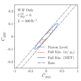
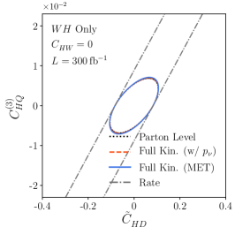
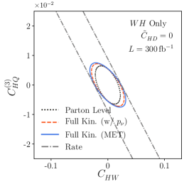
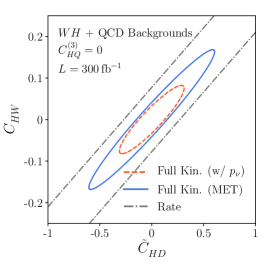
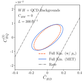
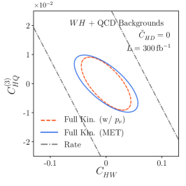
Figure 1: 95% CL limits based on the (linearized) Fisher information on pairs of Wilson coefficients with $\Lambda=1$ TeV, for $WH$ production only (top) and including the QCD background (bottom). We include full parton-level information without detector effects (dotted black), detector effects, but retaining the full neutrino 4-momentum (dashed orange), and finally retaining only the transverse neutrino momentum (solid blue). We also show the information using only the signal rate in grey.

Fisher information calculations for fully reconstructable signals and their irreducible backgrounds, also including leading detector effects, have been studied in the past Brehmer:2016nyr ; Brehmer:2017lrt . Using MadMiner we can also study signatures which cannot be fully reconstructed. Specifically in the $WH$ production process, we study the information based on the smeared missing transverse energy rather than the full neutrino momentum. In this section we analyze the loss of information due to these detector effects, comparing three sets of observables: first, keeping the full information on all initial and final state particles at parton level, second, using all final state particles after detector smearing, and third, keeping only the observable missing transverse momentum in place of the neutrino momentum, including all detector-level smearing.

To gain some intuition about the impact of detector effects on the information content of the hard process we analyze two of the three operators given in Eq. (5) at a time, setting the third Wilson coefficient to zero. We also limit ourselves to linearized differential cross sections in each of the Wilson coefficients at this point, the effects of the squared terms will be discussed in detail later.

In Fig. 1 we show how the full information about the dimension-6 signal at the parton level is reduced when we move from parton-level truth to realistic observables step by step. The dotted black line corresponds to retaining the full parton-level information without detector effects that is used for the evaluation of the matrix elements. This includes unobservable degrees of freedom such as the initial-state parton flavors, particle helicities and the un-smeared momenta. Removing this information and introducing a realistic smearing of the particle momenta washes out possible structures, for example asymmetries in the rapidity distributions, as can be seen when going from the black to the orange line. In this step we still assume that we can measure the full neutrino four-momentum. Finally, we remove the unobserved longitudinal neutrino momentum and neutrino energy, which changes the orange line into the blue line. While the longitudinal neutrino momentum can in principle be reconstructed if we assume an on-shell $W$ boson, this reconstruction is spoiled by the detector smearing.

In the top panels of Fig. 1, we neglect the QCD backgrounds and consider only $WH$ production with linear dimension-six contributions. The loss of information has the strongest impact on the correlated measurements of $\tilde{C}_{HD}$-$C_{HW}$, because the phase-space effects of both operators are very SM-like. In this situation we rely on the best possible understanding of the full final state. In the $\tilde{C}_{HD}$-$C_{Hq}^{(3)}$ and $C_{HW}$-$C_{Hq}^{(3)}$ planes, we know that the phase-space effects are more dramatic, so the additional information from the third neutrino direction is less relevant. We also show the information from the total rate measurement, which is not only much poorer, but it also shows a perfect flat direction for each pair of operators.

In the lower panel of Fig. 1 we show the same change in available information at detector level, now in the presence of the QCD backgrounds. In this situation, a complete understanding of the final state neutrinos is desirable for understanding small changes in the full phase space distribution due to BSM effects, and hence the missing information affects all three operators.

5.2 Distribution of information

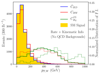
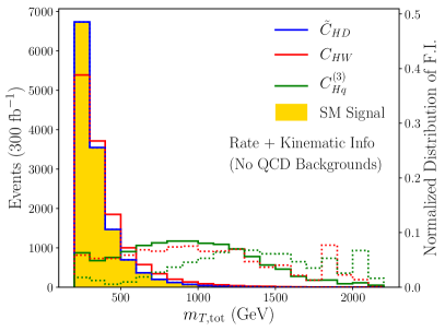
Figure 2: Left axis: SM signal distribution. Right axis: normalized distributions of the diagonal elements of the Fisher information, representing the information on the three Wilson coefficients in bins of $p_{T,W}$ (left panel) and $m_{T,\mathrm{tot}}$ (right panel). The solid lines are linearized in the Wilson coefficients, while the dotted lines show the information on the dimension-6 squared terms.

From Sec. 2 we know that the three dimension-6 operators we are considering have distinctly different effects on the $WH$ production process. If we want to exploit the momentum enhancement of $C_{Hq}^{(3)}$, it is clear that the leading kinematic variable for the partonic $2\to 2$ signal is the partonic energy or equivalently Biekotter:2016ecg

$$p_{T,W}\approx p_{T,H}\quad\text{or}\quad m_{WH}\;.$$ (16)

This simple description as a $2\to 2$ process is broken by two aspects, the $2\to 3$ structure of the $Wb\bar{b}$ continuum background and angular correlations reflecting the $W$ polarization.

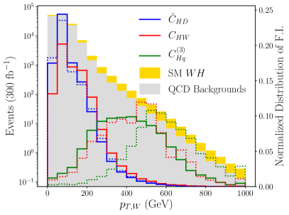
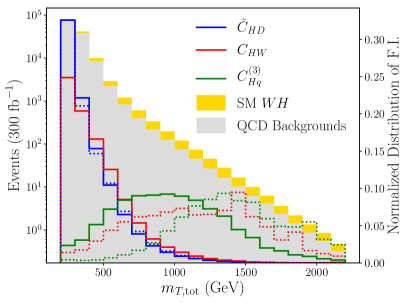
Figure 3: Left axis: stacked histograms of the SM signal on top of the QCD backgrounds for $p_{T,W}$ (left) and $m_{T,\text{tot}}$ (right). Right axis: normalized distributions of the diagonal elements of the Fisher information, representing the information on the three Wilson coefficients. The solid lines are linearized in the Wilson coefficients, while the dotted lines show the information on the dimension-6 squared terms.

In the left panel of Fig. 2, we show the $p_{T,W}$ distribution for the $WH$ signal, together with the information distribution. We start with the normalized distribution of the diagonal element of the Fisher information introduced in Sec. 4.2, by definition linearized in the Wilson coefficient, as solid lines. These curves correspond to the diagonal elements of the Fisher Information matrix computed using only events that lie within the bin boundaries for a chosen kinematic variable. These diagonal elements are inversely proportional to the estimated limit on the theory parameter, and the full information (and optimal limit) can be obtained by adding up the information in each bin. The distributions thus demonstrate where in phase space the constraining power on each Wilson coefficient arises, and where the experimental analyses should be focused.

We see that the information on all three operators reflects their respective Lorentz structures. The information on $\tilde{\mathcal{O}}_{HD}$ mimics the distribution of the signal, and the information in $\mathcal{O}_{HW}$ is energy-suppressed because it couples to the transverse $W$-modes. In contrast, $\mathcal{O}_{Hq}^{(3)}$ is visible at large momentum transfer because of the 4-point vertex.

In the same figure we also show the information distribution as dotted lines for the dimension-6 squared terms only for each of the three operators. In this case the interference with the Standard Model does not act as a projector onto the $W$-polarization structure of the Standard Model. In these plots we treat the squared Wilson coefficients as unconstrained parameters; physically, they are restricted to be non-negative, but this does not change our conclusions. What we see clearly is that the sensitive phase-space region for $\mathcal{O}_{HW}$ now peaks around 400 GeV, well outside the dominant phase-space region of the SM signal. Also the peak in the information on $\mathcal{O}_{Hq}^{(3)}$ moves from around 400 GeV to 600 GeV, dominated by the squared 4-point vertex.

The right panel of Fig. 2 shows the distribution and information distribution over the total transverse mass of the final state,

$$m_{T,\text{tot}}=\sqrt{\left(E_{T}^{bb\ell}+\not{E}_{T}\right)^{2}-\left|\mathbf{p}_{T}^{bb\ell}+\not{\mathbf{p}}_{T}\right|^{2}}\;,$$ (17)

where $E_{T}^{bb\ell}=\sqrt{|\mathbf{p}_{T}^{bb\ell}|^{2}+m^{2}_{bb\ell}}$ and $\mathbf{p}_{T}^{bb\ell}$ is the vector sum of the transverse momenta of the lepton and the $b$-jet, with similar conclusions.

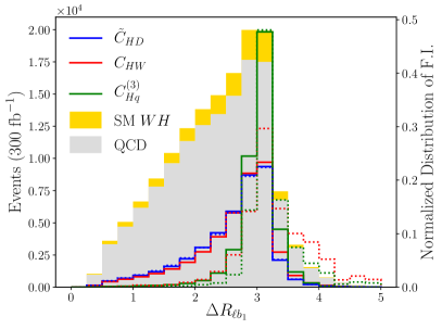
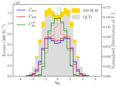
Figure 4: Left axis: stacked histograms of the SM signal on top of the backgrounds for different kinematic observables. Right axis: normalized distributions of the diagonal elements of the Fisher information, representing the information on the three Wilson coefficients.

In Fig. 3, we demonstrate how including the continuum QCD background changes the picture. First, we see that regions of low $p_{T}$ or low $m_{T,\text{tot}}$ are swamped by the QCD backgrounds, so they do not lend themselves to extracting momentum-enhanced contributions. For $\tilde{\mathcal{O}}_{HD}$ there is no momentum enhancement, and the information in the two distributions behaves exactly as before. Similarly, the information distribution on $\mathcal{O}_{HW}$ in the linear case is primarily in the low bins, where the event rate is larger, but is largest for $p_{T,W}\gtrsim 300$ or $m_{T,\text{tot}}\gtrsim 700$ GeV if we consider the dimension-6 squared term. In contrast, $\mathcal{O}_{Hq}^{(3)}$ gains only very little information from the low-$p_{T,W}$ or low-$m_{T,\text{tot}}$ regime. We note that for operators only affecting the total rate, the distribution of information over $p_{T,W}$ is completely consistent with the distribution of the statistical significance of the $VH$ production over the QCD background, as studied in Ref. Plehn:2013paa .

Here we pause to comment on the validity of the EFT expansion. While for each operator, only the combination $C_{i}/\Lambda^{2}$ is observable, matching with a perturbative theory at higher scales requires $C_{i}\lesssim 1$, and thus more precise measurements are intrinsically probing potentially higher scales. In order for the constraints to be self-consistent, it is important that we do not try to set constraints on the EFT parameters using data that is outside the range of validity of the EFT expansion. This could be done rigorously by implementing a cut demanding that some kinematic variable tracing the momentum transfer not exceed some multiple of $\Lambda$, but fortunately, in Fig. 3, we see that all of the Information arises from events with $p_{T,W}\lesssim 1\,\mathrm{TeV}$, so such a cut is unnecessary for our analysis here.

Finally, in Fig. 4 we consider two more kinematic distributions. First, the opening angle of the charged lepton and the leading bottom becomes $\Delta R_{\ell b_{1}}\approx\pi$ for boosted $2\to 2$ processes, like the part of $WH$ phase space sensitive to $\mathcal{O}_{Hq}^{(3)}$. Second, the reconstructed rapidity of the $b\bar{b}$ system also becomes more central for boosted $2\to 2$ processes. The opening angle is useful for discriminating against the $t\bar{t}$ and $tb$ backgrounds, where we do not expect the two $b$-jets to recoil against the lepton, but they do not otherwise appear too promising to gain additional information into one of the three dimension-6 operators, or into the relation between linearized and quadratic contributions.

Altogether, we have learned that when looking at 1D kinematic distributions those which scale like momentum, like $p_{T}$ or $m_{T,\text{tot}}$, are best-suited to separate the effects of the different operators. Including QCD backgrounds makes the high-momentum regime even more attractive. The only problem is that the relevant region, for instance in $p_{T,W}$, depends not only on the operator, but also on whether we linearize the effective field theory for the cross section or keep the ${\cal{O}}({1/\Lambda^{4}})$ squared term. Furthermore, the balance between linear and quadratic contributions to a combined analysis will change with the LHC luminosity and the kinematic focus of the analysis.

5.3 Information in STXS

Testing one effective operator at a time violates the basic assumptions of effective theories, namely that we expect to see effects from all operators allowed by the underlying theory. We now examine how the kinematic variables introduced in the previous section can be used to set constraints on the full multi-dimensional parameter space.

Simplified template cross sections (STXS) have been proposed to provide experimental results on kinematic distributions for global analyses Tackmann:2138079 ; Berger:2019wnu . For the $WH$ production process they include rate measurements binned in $p_{T,W}$. At stage 1, the three bins are defined by $p_{T,W}=0-150$ GeV, $p_{T,W}=150-250$ GeV, and $p_{T,W}>250$ GeV. For increased statistics, stage 1.1 proposes five bins, now split at $p_{T,W}=75,150,250,400$ GeV, as shown in Fig. 7. Results using this approach have recently been presented by ATLAS Aaboud:2019nan using the 0-jet, single lepton data sample, to obtain limits on anomalous couplings, assuming only one non-zero Wilson coefficient at a time. Unfortunately, they do not consider the most interesting 4-point vertex from $\mathcal{O}_{Hq}^{(3)}$, for which boosted $VH$ production provides the strongest constraints Biekotter:2018rhp .

We evaluate these proposals by calculating the Fisher information in the STXS bins. From Fig. 3, it is clear that the stage 1.1 STXS version will not capture the full information on $\mathcal{O}_{Hq}^{(3)}$, so we consider a 6-bin setup with

$$p_{T,W}^{\text{bins}}=(\,0-75,\,75-150,\,150-250,\,250-400,\,400-600,\,600-\infty\,)~{}{\rm GeV}\;.$$ (18)

We compare the results to the full information in the high-dimensional phase space using the Sally method discussed in Sec. 4.1. In addition, we train a neural network with the Sally method on just $p_{T,W}$ as input variable, which lets us calculate the information in the full $p_{T,W}$ distribution in the infinite-bin limit; see App. D for more details.

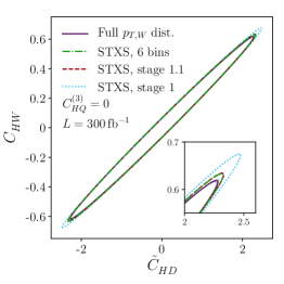
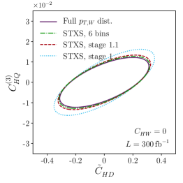
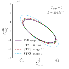
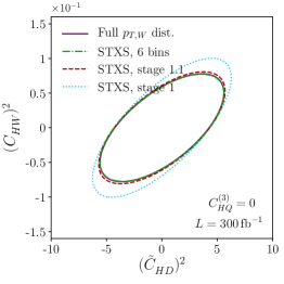
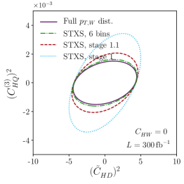
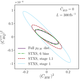
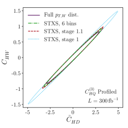
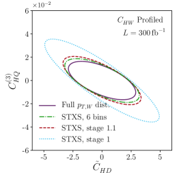
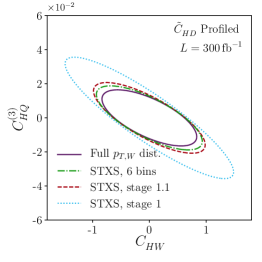
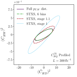
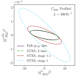
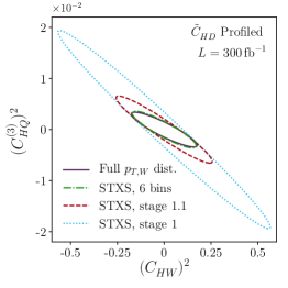
Figure 5: 95% CL constraints based on $p_{T,W}$ in the Fisher information approximation. We show linearized and squared-only results setting the third operator to zero (top six panels) and profiling over the third operator (bottom six panels). The blue dotted line shows the STXS stage 1 (3 bins), red dashed stage 1.1 (5 bins), and green dot-dashed and purple solid show the results when adding a 6th bin or including the full $p_{T,W}$ distribution.

In Fig. 5, we show the expected limits on pairs of Wilson coefficients from the $p_{T,W}$ distribution. First, we see the almost flat direction in the $\tilde{\mathcal{O}}_{HD}-\mathcal{O}_{HW}$ plane, reflecting the fact that both operators are constrained at low transverse momenta, as long as we only consider linearized predictions. This flat direction will be broken by other observables in a proper global analysis Biekotter:2018rhp , so it is of less interest for our purposes. The situation changes once we consider the correlation of either of these two operators with $\mathcal{O}_{Hq}^{(3)}$, because now the two directions are tested by distinctly different $p_{T,W}$ regimes. The only requirement in this case is that we include enough $p_{T,W}$ bins to distinguish the two regimes, as is provided by the stage 1.1 setup. Indeed, this framework collects essentially all information on our set of three operators affecting the $p_{T,W}$ distribution.

In the second row of Fig. 5 we switch from the linear terms in the Wilson coefficient to the squared terms alone, as defined in Section 4.3. This allows us to analyze the relative sensitivity of the different analysis strategies and binnings on the squared terms which, as we saw in Figs. 3 and 4, have very different kinematic behaviors compared to the linear terms. Showing the information on the squared terms as contours also allows us to study the correlations between different squared parameters, which, as we will see, are often different than the correlations between linear terms. In the left panel we see hardly any effect of the different binnings for $\tilde{\mathcal{O}}_{HD}$, but the flat direction has vanished and the reach in $\mathcal{O}_{HW}$ is increased dramatically by including the high $p_{T,W}$ bins. Because this sensitivity to $\mathcal{O}_{HW}$ comes from high momentum transfer, we start to observe a strong anti-correlation with $\mathcal{O}_{Hq}^{(3)}$. To break it, we need to resolve the high-$p_{T,W}$ range, and for this purpose the additional bin in Eq. (18) is crucial. Indeed, we see that it improves the situation considerably.

In the lower six panels of Fig. 5 we show the same kind of information, but now profiled over the respective third operator. The results are generally much weaker, and the flat directions are more significant. As mentioned above, this is not a big concern, since our $WH$ analysis has to be embedded in a global analysis. An interesting aspect is that with three operators actually contributing to the analysis the gap between the few-bins STXS approach and the full information from the entire $p_{T,W}$ distribution widens. Some details on the scaling with larger number of bins and on the number of bins needed to saturate the information in a kinematic distribution are given in App. D. Altogether, it becomes even more important that we extract as much information for instance on $\mathcal{O}_{Hq}^{(3)}$ by sufficiently covering the dedicated phase-space regions.

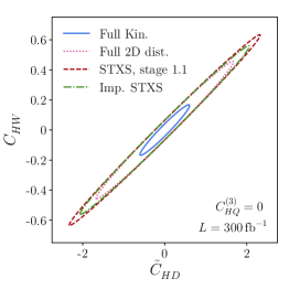
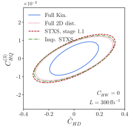
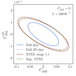
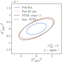
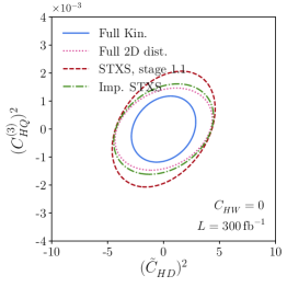
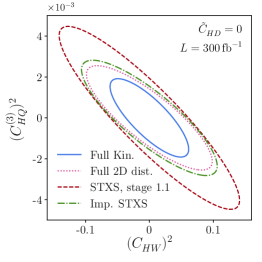
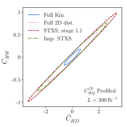
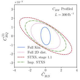
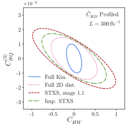
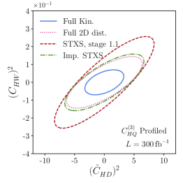
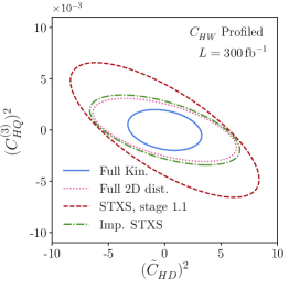
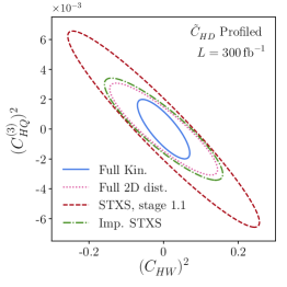
Figure 6: As Fig. 5, now comparing various approaches: The solid blue curve shows the limits from training on the full phase space. The dotted pink line shows training only on the $p_{T,W}$ vs $m_{T,\text{tot}}$ histogram. The limits obtained from the STXS stage 1.1 are shown in dashed red, and the dot-dashed green curve shows the limits obtained by six $p_{T,W}$ bins subdivided into three $m_{T,\text{tot}}$ bins.

After having established that the currently used STXS for $WH$ production need to be supplemented by another high-energy bin, we can test how much of the available information of the full phase space is captured in the binned $p_{T,W}$ distribution. The reasoning behind picking an additional observable scaling like momentum is that the signal process is dominantly $2\to 2$ scattering, described by two kinematic observables, and the scattering angle or rapidity are not found to be particularly useful, as shown in Fig. 4. On the other hand, if the signal from dimension-6 operators populates phase space far away from the SM we will become sensitive to the background kinematics, and the simple picture of a $2\to 2$ process can completely change Plehn:2013paa ; Kling:2016lay .

In the top row of Fig. 6 we show the limits from the Sally approach trained on linearized effects in the Wilson coefficients (the same as in Fig. 1) as a blue line. The dotted pink line comes from limiting the information of the Sally training to the observables $p_{T,W}$ and $m_{T,\text{tot}}$, which can be understood as the constraints computed from the infinite-bin limit of a 2-dimensional histogram. It is not clear a priori which second observable complements $p_{T,W}$ best, but we found that $m_{T,\text{tot}}$ as defined in Eq. (17) works well. In the linearized approach, we confirm that compared to the full phase space we still lose a significant amount of information on the three operators. The next question is how much of the information from the two-dimensional contribution we can capture in a reasonable number of STXS bins. Motivated by Fig 3, we propose to further split each of the six bins in $p_{T,W}$ into three $m_{T,\text{tot}}$ bins in

$$m_{T,\text{tot}}^{\text{bins}}=(\,0-400,\,400-800,\,800-\infty\,)~{}{\rm GeV}\;,$$ (19)

as illustrated in Fig. 7. Because $m_{T,\text{tot}}$ and $p_{T,W}$ are by no means uncorrelated, this captures the effects of the $2\to 3$ background phase space and adds an implicit sub-division in $p_{T,W}$. In the top row of Fig. 6, we see that for the linearized case our new proposed STXS definition performs extremely well, but the STXS stage 1.1 also does fine. In the second row, we show the same effects, but now for the squared new physics terms only and not including the imposed positivity condition. The blue curve is now generated consistently based on the squared terms, using the Harry method. As expected, the improved 2-dimensional STXS outperform the stage 1.1 results when we test $\mathcal{O}_{Hq}^{(3)}$, as a better understanding of the information in high $p_{T,W}$ or $m_{T,\text{tot}}$ bins is effective. The lower panels of Fig. 7 show the same effect, but profiled over the full range of the respective third Wilson coefficient. The large effect related to $\mathcal{O}_{Hq}^{(3)}$ now propagates through the entire set of measurements. Moreover, the limited number of bins in the STXS stage 1.1 become an issue.

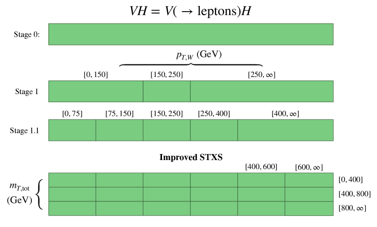
Figure 7: Definition of the old STXS Tackmann:2138079 ; Berger:2019wnu and our proposed improved version based on Eqs. (18) and (19).

5.4 Limits with consistent squared terms

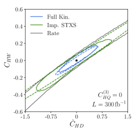
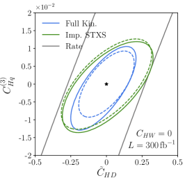
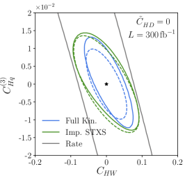
Figure 8: Expected exclusion limits at 95% CL based on a rate-only analysis (grey), from the improved STXS (green), and from a multivariate analysis of the full phase-space information with the Sally algorithm. We show (linearized) limits based on the Fisher information (dashed) and full exclusion limits that take into account the effects of linearized and squared new physics effects (solid). In each panel, we set the operator not shown to zero.

Finally, we go beyond the linearized Fisher-information approach and calculate expected exclusion limits on the dimension-6 Wilson coefficients with the squared terms included in a physically consistent way. Generally, power counting in $1/\Lambda^{2}$ suggests that the linear effects should be dominant. However, in some directions of parameter space the interference contribution to the analyzed distributions is small, the analysis is only sensitive further away from the SM, and the squared terms are the dominant effects of new physics. We thus expect the squared terms to break the flat directions of the linearized results.

This is exactly what we find in Fig. 8, where we show the expected limits for a rate-only analysis (gray), the improved STXS defined in the previous section (green), and a multivariate analysis of the full phase-space information based on the Sally technique described in Sec. 4.1 (blue). In the plane spanned by $\tilde{C}_{HD}$ and $C_{HW}$ (left panel) we can clearly see that the squared contributions remove the approximate flat direction in the improved STXS limits. More generally, the full exclusion limits based on the Sally method differ from those obtained from the linearized Fisher information, indicating the importance of squared new physics effects in this region of parameter space. In these parameter-space regions we expect that even stronger limits can be constructed with techniques that estimate the full likelihood function to all orders in the Wilson coefficients Brehmer:2018hga ; Brehmer:2018kdj ; Brehmer:2018eca ; Brehmer:2019xox . Closer to the SM, we find that the full limits are well approximated by the Fisher information, confirming that the linear operator effects dominate there. Generally, these full limit calculations confirm the main result of the last section: the simplified template cross sections, in particular our improved version, are substantially more informative than a simple rate measurement, but fall short of capturing all of the kinematic information in the high-dimensional final state.

There are numerous global studies that compare the sensitivity to various coefficients at LEP and at the LHC Ellis:2018gqa ; Berthier:2016tkq ; Almeida:2018cld ; Grojean:2018dqj ; Biekotter:2018rhp , as well as studies examining the reach of the $VH$ processes separately Banerjee:2018bio ; Franceschini:2017xkh ; Freitas:2019hbk . The global Warsaw basis fit of Ref. Ellis:2018gqa finds single parameter fits which are roughly consistent with our improved STXS projections of Fig. 8. Our results should be interpreted as demonstrating the potential improvements in precision fits that could be obtained by improving the binning or by adding information from additional kinematic variables.

6 Conclusions

We have, for the first time, performed a comprehensive benchmarking of simplified template cross sections (STXS) in the $WH$ channel with a leptonic $W$ decay. The Fisher information allowed us to quantify the reach of different analysis strategies and to identify which phase-space regions are sensitive to the three dimension-6 operators $\tilde{\mathcal{O}}_{HD}$, $\mathcal{O}_{HW}$, and $\mathcal{O}_{Hq}^{(3)}$. We compared the STXS to a machine-learning-based analysis of the full, high-dimensional final state, using the Sally technique of Refs. Brehmer:2018hga ; Brehmer:2018kdj ; Brehmer:2018eca implemented in MadMiner Brehmer:2019xox to calculate the statistically optimal observables and the maximal new physics reach of an analysis.

We found that $p_{T,W}$ is the most promising kinematic observable, but that the STXS stage 1.1 criteria benefit from being supplemented by an additional high-energy bin. The ability to distinguish different operator signatures is further enhanced when we include a second observable in the definition of the STXS, $m_{T,\text{tot}}$ being one workable option. We showed that for the $WH$ process such a two-dimensional approach is promising, even though it cannot obtain all of the kinematic information in the process that can be unearthed with machine-learning-based techniques. Our results suggest, however, that the current STXS results can be significantly improved by the two-dimensional binning. More generally, this study presents a blueprint for a systematic benchmarking of STXS or any other method of publishing results needed for a global Higgs analysis.

Acknowledgments

We would like to thank Anke Biekötter, Sebastian Bruggisser, and Lukas Heinrich for useful discussions. We are grateful to Kyle Cranmer, whose ideas laid the foundation for our statistical analysis. We acknowledge the use of Delphes 3 deFavereau:2013fsa , Jupyter notebooks Kluyver2016JupyterN , MadGraph5_aMC Alwall:2014hca , MadMiner Brehmer:2019xox ; madminer , Matplotlib Hunter:2007 , NumPy numpy , pylhe lukas_2018_1217032 , Pythia 8 Sjostrand:2014zea , Python van1995python , PyTorch paszke2017automatic , scikit-hep Rodrigues:2019nct , scikit-learn scikit-learn , and uproot jim_pivarski_2019_3256257 .

The work of JB is supported by the U. S. National Science Foundation (NSF) under the awards ACI-1450310, OAC-1836650, and OAC-1841471, and by the Moore-Sloan data science environment at NYU. The work of SH is supported by the NSF grant PHY-1620628 and the U.S. Department of Energy, Office of Science, Office of Workforce Development for Teachers and Scientists, Office of Science Graduate Student Research (SCGSR) program. The SCGSR program is administered by the Oak Ridge Institute for Science and Education (ORISE) for the DOE. ORISE is managed by ORAU under contract number DE-SC0014664. The work of FK is supported by NSF grant PHY-1620638 and U. S. Department of Energy grant DE-AC02-76SF00515. TP’s research is supported by the German DFG Collaborative Research Centre P3H: Particle Physics Phenomenology after the Higgs Discovery (CRC TRR 257). This work was supported through the NYU IT High Performance Computing resources, services, and staff expertise. The work of SD is supported by the U. S. Department of Energy under Grant DE-SC0012704.

Our analysis code is available online at Ref. repo .

Appendix A Detector effects

The leading detector effect relevant for this analysis is the smearing of the di-jet invariant mass peak. The distribution has been carefully simulated by CMS CMS:2018abb (see Fig. 9) and we aim to reproduce it for our analysis. In the MadMiner framework, this smearing can be simulated in three different ways: i) In the simplest approach, we explicitly smear the parton level $b$-quark energies after event generation. This is parameterized by a gaussian transfer function with width $\sigma_{E}/E=0.1$. ii) Alternatively, we can include the smearing already in the event generation process by modifying the Higgs propagator Brehmer:2017lrt ; Brehmer:2016nyr ; Kling:2016lay . To reproduce the $m_{bb}$ distribution obtained by CMS, the Breit-Wigner propagator is simply replaced by the square-root of the Gaussian with mean $m_{H}$, and width $\sigma=15$ GeV. As a result, the joint scores already include the smearing and can therefore be used as estimator for the score, making this approach a useful tool for validation (see Appendix B). iii) Finally, it is also possible to simulate parton shower, hadronization and detector response using Pythia and Delphes.

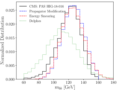
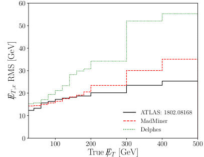
Figure 9: Left: Invariant di-jet mass $m_{bb}$ from Higgs decay obtained by CMS CMS:2018abb (solid black), the parton level energy smearing (dashed red), the modified Higgs propagator smearing (dashed blue), and a simulation of shower and detector response with Pythia 8 and Delphes 3 (green dotted). Right: RMS of the missing transverse momentum smearing in the x-direction, $/\!\!\!\!E_{T,x}$, as a function of the true missing energy $\not{E}_{T}$ for the signal process obtained by ATLAS Aaboud:2018tkc (solid black), the MET smearing in MadMiner, (dashed red) and by a simulation of shower and detector response with Pythia 8 and Delphes 3 (dotted green).

In the left panel of Fig. 9 we compare the three approaches to the di-jet mass distribution obtained by CMS CMS:2018abb (solid black). We can see that both the parton level energy smearing (dashed red) and propagator modifcation (dashed blue) approach can reproduce the CMS mass spectrum, while a fast detector simulation using Pythia 8 Sjostrand:2014zea and Delphes 3 deFavereau:2013fsa with default settings (dotted green) systematically underestimates the di-jet mass.

Another important detector effect is the smearing of the missing transverse energy $\not{E}_{T}$. In this work, we aim to reproduce the most recent ATLAS performance Aaboud:2018tkc and explicitly smear the transverse components of the missing energy using a Gaussian transfer function with width $\sigma_{\not{E}_{T}}=12.5~{}{\rm GeV}$. An additional smearing at higher energies is induced through the smearing of the $b$-quark energies. As shown in the right panel of Fig. 9, this procedure reproduces the experimental results well. In contrast, a fast detector simulation using Pythia 8 and Delphes 3 once again fails to accurately reproduce the experimental performance without tuning the simulation parameters, as indicated by the green dotted line.

Appendix B Fisher information in the presence of backgrounds

A key feature of the machine learning approach in MadMiner is that one can reliably estimate the score in the presence of backgrounds. As explained in Ref. Brehmer:2019xox , this also works when signal and background samples are generated separately from each other, implicitly inducing an additional discrete latent variable which labels each training event as either signal or background. This latent variable is then integrated out in the machine learning step alongside with all other unobservable latent variables, such as the longitudinal neutrino momenta, initial state quark flavours or additional unobserved particles in reducible backgrounds (such as the jets in top pair production). Reference Brehmer:2019xox contains examples to validate the performance of MadMiner’s machine learning approach in the case of either a single observable or a single process. In the following, we will consider another simplified scenario in which we can validate MadMiner’s reach estimate in the presence of both a high-dimensional observable space and irreducible backgrounds.

As mentioned in Sec. 4.2, for a fixed initial and final state at parton level, we can calculate the Fisher information directly from the event weights and hence cross check the machine learning based results. In particular, we consider the process $u\bar{d}\to\mu^{+}\nu\,b\bar{b}$, with contributions coming from both the $WH$ signal and the irreducible $Wb\bar{b}$ background, and restrict ourselves to only two effective operators $\mathcal{O}_{HD}$ and $\mathcal{O}_{Hq}^{(3)}$. We first generate a set of signal events $\{x_{k}\}$, described by event weights $\Delta\sigma_{S,k}(\theta)$. In contrast to the results in Section 3, where the smearing of the $m_{bb}$ peak was done at analysis level, here we generate the signal events using the propagator modification method described in Appendix A. We then use the MadGraph reweighting tool Mattelaer:2016gcx to obtain the background weights $\Delta\sigma_{B,k}$ for the same set of events. As shown in Ref. Brehmer:2016nyr , the Fisher information at parton level for a set of events can then be computed as

$$I_{ij}=\sum_{\text{events, }k}\frac{\mathcal{L}}{\Delta\sigma_{k}(0)}\frac{\partial\Delta\sigma_{k}(\theta)}{\partial_{\theta_{i}}}\Bigg{|}_{\theta=0}\frac{\partial\Delta\sigma_{k}(\theta)}{\partial_{\theta_{j}}}\Bigg{|}_{\theta=0}\;.$$ (20)

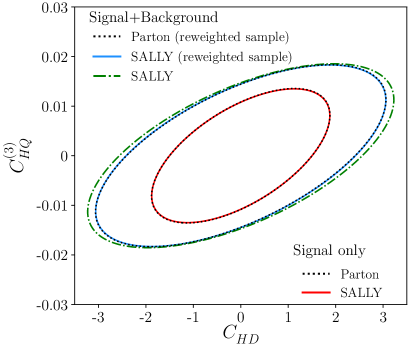
Figure 10: A comparison of the 95% CL limits based on the Fisher information in the two-parameter space for a simplified version of our process, comparing the Fisher information obtained from a set of parton level event weights (dotted lines), using a Sally estimator trained on the same sample events (solid lines), and using a Sally estimator trained on separate signal and background event samples (dot-dashed line). The inner ellipses show the results when evaluated only on the signal sample, while the outer ellipses show the results taking into account both signal and background.

A comparison of the Fisher information obtained using machine learning results with the Fisher information directly obtained from the parton level event weights is shown in Fig. 10. The inner ellipses show the reach in the absence of backgrounds ($\Delta\sigma_{k}=\Delta\sigma_{S,k}$), while the outer ellipses take into account both signal and background ($\Delta\sigma_{k}=\Delta\sigma_{S,k}+\Delta\sigma_{B,k}$). In both cases, the Fisher information obtained at parton level (dotted curves) and using a Sally estimator trained on the same sample (solid curves) are indistinguishable, indicating excellent machine learning performance. This is then compared to the standard way of estimating the Fisher information, using a Sally estimator trained with separately generated signal and background samples, which is indicated by the green dot-dashed ellipse. This result agrees remarkably well with the other results, confirming that the treatment of backgrounds in the MadMiner algorithm works correctly.

Appendix C Systematics

An important question that must be addressed when comparing the expected limits from different sets of kinematic data from experiments is the effect of systematic uncertainties on the expected limits. While a treatment of all experimental systematics is beyond the scope of this study, an important step in this direction is to understand the effects of theory uncertainties, namely the dependence on the choice of renormalization and factorization scales as well as the PDFs. These uncertainties are fully integrated in the MadMiner framework Brehmer:2019xox and parameterized through nuisance parameters, which are then marginalized over to set limits.

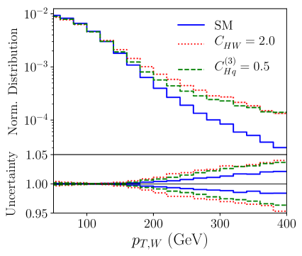
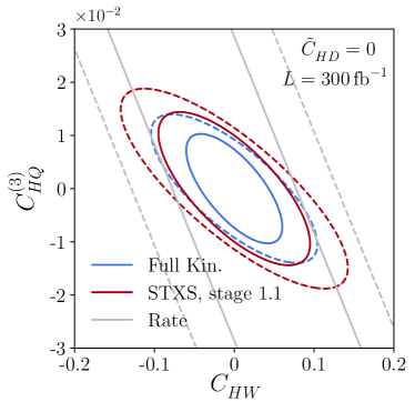
Figure 11: Left: The normalized distributions of $p_{T,W}$ for signal and background weights with various choices of the theory parameters and (barely visible) shaded bands showing the effects of the PDF and scale uncertainties. Right: The 95% CL bounds on $C_{HW}$ and $C_{Hq}^{(3)}$ in the Fisher information approximation obtained with the Sally estimator evaluated using the full set of physical variables (blue), the Stage 1.1 simplified template cross sections (red), and measurements of the rate (grey), with $\tilde{C}_{HD}$ fixed to zero. The solid lines show the projected limits obtained in the absence of systematic uncertainties, while the dashed lines show the reach contours after marginalizing over the additional nuisance parameters.

In the following we only consider the theory uncertainties on the $WH$ signal. Since uncertainties on the backgrounds are typically mitigated through the use of sideband analyses, rather than through direct simulations, including the scale and PDF uncertainties on the backgrounds would dramatically overestimate the actual systematic uncertainty in a realistic measurement.

In the left panel of Fig. 11 we show the normalized distribution of the $W$ boson’s transverse momentum including scale and PDF uncertainties for several benchmark parameter points. In particular we vary the renormalization and factorization scale by a factor of two and use the PDF4LHC15_nlo_30 set to estimate PDF uncertainties. We see that the relative uncertainty is small in the background-dominated low-$p_{T,W}$ regime, and increases to $\mathcal{O}(5\%)$ at large transverse momentum. In $WH$ production, the PDF shape uncertainties dominate over the scale uncertainties, given that the scale dependence of the quark PDF is small.

In the right panel of Fig. 11 we show how including systematics changes the expected limits. While the solid contours show the reach neglecting systematic uncertainties, the dashed lines account for the systematic uncertainties by profiling over the nuisance parameters. We can see that the presence of systematic uncertainties mainly reduce the sensitivity in the rate-sensitive direction, rotating the orientation of the ellipses. The overall effect is sizable, indicating the importance of understanding these systematic uncertainties. In Fig. 11, we see that at $p_{T,W}\sim 300-400~{}GeV$, the energy scaling of $C_{HW}$ and $C_{HQ}^{(3)}$ is roughly the same, due to the fact that we are not yet in the high $p_{T,W}$ regime where the longitudinal modes dominate. In this energy range, the transverse modes, that have the same scaling with $\sqrt{s}/M_{W}$, are clearly important.

Appendix D Binning distributions

In view of an appropriate definition of simplified template cross sections, it is interesting to ask how finely we need to bin a kinematic distribution to extract as much of the available information as possible. This is illustrated in Fig. 12, where we show the Fisher information corresponding to a $p_{T,W}$ histogram for varying number of bins with equal size in the range $[0,800~{}\text{GeV}]$. The three panels correspond to the diagonal element of the Fisher information for $\tilde{C}_{HD}$ (left), $C_{HW}$ (center) and $C_{QH}^{(3)}$ (right).

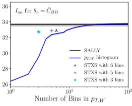
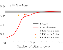
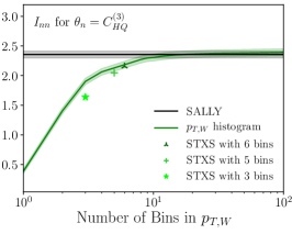
Figure 12: Diagonal elements of Fisher information obtained from a $p_{T,W}$ histogram with varying number of bins. The horizontal black line shows the Fisher information obtained using the Sally method trained only with $p_{T,W}$ as input observable. The markers show the information in the STXS with 3, 5 and 6 bins, respectively.

This is compared to the information obtained using a Sally score estimator trained with only $p_{T,W}$ as input observable (solid black) and the information in the STXS with 3 bins (stars), 5 bins (crosses) and 3 bins (triangles). The shaded regions indicated the uncertainties of the Fisher information, where the uncertainty for the Sally method was estimated using an ensemble of estimators with varying architecture. We can see that the information in histograms approaches the information in the distribution in the limit of large number of bins, showing that the Sally approach gives the correct large-$n_{\text{bin}}$ limit. For all three operators, a histogram with an $\mathcal{O}(10)$ number of bins will essentially extract the full information of the $p_{T,W}$ distribution. The STXS with 3 bins already collects almost all information on $\tilde{C}_{HD}$ and $C_{HW}$, while for $C_{QH}^{(3)}$ a significant improvement is obtained when increasing the number of bins to 6.

References

- (1) S. Dawson, C. Englert and T. Plehn, Higgs Physics: It ain’t over till it’s over, Phys. Rept. 816 (2019) 1 [1808.01324].
- (2) I. Brivio and M. Trott, The Standard Model as an Effective Field Theory, Phys. Rept. 793 (2019) 1 [1706.08945].
- (3) A. Butter, O. J. P. Eboli, J. Gonzalez-Fraile, M. C. Gonzalez-Garcia, T. Plehn and M. Rauch, The Gauge-Higgs Legacy of the LHC Run I, JHEP 07 (2016) 152 [1604.03105].
- (4) I. Brivio, J. Gonzalez-Fraile, M. C. Gonzalez-Garcia and L. Merlo, The complete HEFT Lagrangian after the LHC Run I, Eur. Phys. J. C76 (2016) 416 [1604.06801].
- (5) S. Banerjee, S. Mukhopadhyay and B. Mukhopadhyaya, Higher dimensional operators and the LHC Higgs data: The role of modified kinematics, Phys. Rev. D89 (2014) 053010 [1308.4860].
- (6) S. Di Vita, G. Durieux, C. Grojean, J. Gu, Z. Liu, G. Panico et al., A global view on the Higgs self-coupling at lepton colliders, JHEP 02 (2018) 178 [1711.03978].
- (7) J. Ellis, C. W. Murphy, V. Sanz and T. You, Updated Global SMEFT Fit to Higgs, Diboson and Electroweak Data, JHEP 06 (2018) 146 [1803.03252].
- (8) E. da Silva Almeida, A. Alves, N. Rosa Agostinho, O. J. P. Éboli and M. C. Gonzalez-Garcia, Electroweak Sector Under Scrutiny: A Combined Analysis of LHC and Electroweak Precision Data, Phys. Rev. D99 (2019) 033001 [1812.01009].
- (9) A. Biekötter, T. Corbett and T. Plehn, The Gauge-Higgs Legacy of the LHC Run II, SciPost Phys. 6 (2019) 064 [1812.07587].
- (10) ATLAS collaboration, Reproducing searches for new physics with the ATLAS experiment through publication of full statistical likelihoods, Tech. Rep. ATL-PHYS-PUB-2019-029, CERN, Geneva, Aug, 2019.
- (11) CMS collaboration, Simplified likelihood for the re-interpretation of public CMS results, Tech. Rep. CMS-NOTE-2017-001. CERN-CMS-NOTE-2017-001, CERN, Geneva, Jan, 2017.
- (12) K. Cranmer, S. Kreiss, D. Lopez-Val and T. Plehn, Decoupling Theoretical Uncertainties from Measurements of the Higgs Boson, Phys. Rev. D91 (2015) 054032 [1401.0080].
- (13) E. Maguire, L. Heinrich and G. Watt, HEPData: a repository for high energy physics data, J. Phys. Conf. Ser. 898 (2017) 102006 [1704.05473].
- (14) C. N. Leung, S. T. Love and S. Rao, Low-Energy Manifestations of a New Interaction Scale: Operator Analysis, Z. Phys. C31 (1986) 433.
- (15) W. Buchmuller and D. Wyler, Effective Lagrangian Analysis of New Interactions and Flavor Conservation, Nucl. Phys. B268 (1986) 621.
- (16) M. C. Gonzalez-Garcia, Anomalous Higgs couplings, Int. J. Mod. Phys. A14 (1999) 3121 [hep-ph/9902321].
- (17) C. Grojean, M. Montull and M. Riembau, Diboson at the LHC vs LEP, JHEP 03 (2019) 020 [1810.05149].
- (18) J. de Blas, M. Ciuchini, E. Franco, S. Mishima, M. Pierini, L. Reina et al., Electroweak precision constraints at present and future colliders, PoS ICHEP2016 (2017) 690 [1611.05354].
- (19) F. Tackmann, K. Tackmann, K. Tackmann, M. Duehrssen-Debling and P. Francavilla, Simplified template cross sections, cds.cern.ch/record/2138079.
- (20) N. Berger et al., Simplified Template Cross Sections - Stage 1.1, 1906.02754.
- (21) J. Brehmer, K. Cranmer, F. Kling and T. Plehn, Better Higgs boson measurements through information geometry, Phys. Rev. D95 (2017) 073002 [1612.05261].
- (22) J. Brehmer, F. Kling, T. Plehn and T. M. P. Tait, Better Higgs-CP Tests Through Information Geometry, Phys. Rev. D97 (2018) 095017 [1712.02350].
- (23) J. Brehmer, K. Cranmer, G. Louppe and J. Pavez, A Guide to Constraining Effective Field Theories with Machine Learning, Phys. Rev. D98 (2018) 052004 [1805.00020].
- (24) J. Brehmer, K. Cranmer, G. Louppe and J. Pavez, Constraining Effective Field Theories with Machine Learning, Phys. Rev. Lett. 121 (2018) 111801 [1805.00013].
- (25) J. Brehmer, G. Louppe, J. Pavez and K. Cranmer, Mining gold from implicit models to improve likelihood-free inference, 1805.12244.
- (26) J. Brehmer, F. Kling, I. Espejo and K. Cranmer, MadMiner: Machine learning-based inference for particle physics, 1907.10621.
- (27) F. F. Freitas, C. K. Khosa and V. Sanz, Exploring SMEFT in VH with Machine Learning, 1902.05803.
- (28) T. Corbett, O. J. P. Eboli, J. Gonzalez-Fraile and M. C. Gonzalez-Garcia, Robust Determination of the Higgs Couplings: Power to the Data, Phys. Rev. D87 (2013) 015022 [1211.4580].
- (29) B. Grzadkowski, M. Iskrzynski, M. Misiak and J. Rosiek, Dimension-Six Terms in the Standard Model Lagrangian, JHEP 10 (2010) 085 [1008.4884].
- (30) I. Brivio and M. Trott, Scheming in the SMEFT… and a reparameterization invariance!, JHEP 07 (2017) 148 [1701.06424], [Addendum: JHEP05,136(2018)].
- (31) L. Berthier, M. Bjorn and M. Trott, Incorporating doubly resonant data in a global fit of SMEFT parameters to lift flat directions, JHEP 09 (2016) 157 [1606.06693].
- (32) J. Haller, A. Hoecker, R. Kogler, K. Monig, T. Peiffer and J. Stelzer, Update of the global electroweak fit and constraints on two-Higgs-doublet models, Eur. Phys. J. C78 (2018) 675 [1803.01853].
- (33) A. Dedes, W. Materkowska, M. Paraskevas, J. Rosiek and K. Suxho, Feynman rules for the Standard Model Effective Field Theory in Rξ -gauges, JHEP 06 (2017) 143 [1704.03888].
- (34) J. Nakamura, Polarisations of the and bosons in the processes and , JHEP 08 (2017) 008 [1706.01816].
- (35) J. Alwall, R. Frederix, S. Frixione, V. Hirschi, F. Maltoni, O. Mattelaer et al., The automated computation of tree-level and next-to-leading order differential cross sections, and their matching to parton shower simulations, JHEP 07 (2014) 079 [1405.0301].
- (36) J. Butterworth et al., PDF4LHC recommendations for LHC Run II, J. Phys. G43 (2016) 023001 [1510.03865].
- (37) V. Hirschi and O. Mattelaer, Automated event generation for loop-induced processes, JHEP 10 (2015) 146 [1507.00020].
- (38) I. Brivio, Y. Jiang and M. Trott, The SMEFTsim package, theory and tools, JHEP 12 (2017) 070 [1709.06492].
- (39) ATLAS collaboration, Observation of decays and production with the ATLAS detector, Phys. Lett. B786 (2018) 59 [1808.08238].
- (40) CMS collaboration, Observation of Higgs boson decay to bottom quarks, Phys. Rev. Lett. 121 (2018) 121801 [1808.08242].
- (41) ATLAS collaboration, Performance of missing transverse momentum reconstruction with the ATLAS detector using proton-proton collisions at = 13 TeV, Eur. Phys. J. C78 (2018) 903 [1802.08168].
- (42) K. Cranmer and T. Plehn, Maximum significance at the LHC and Higgs decays to muons, Eur. Phys. J. C51 (2007) 415 [hep-ph/0605268].
- (43) D. Atwood and A. Soni, Analysis for magnetic moment and electric dipole moment form-factors of the top quark via , Phys. Rev. D45 (1992) 2405.
- (44) M. Davier, L. Duflot, F. Le Diberder and A. Rouge, The Optimal method for the measurement of tau polarization, Phys. Lett. B306 (1993) 411.
- (45) M. Diehl and O. Nachtmann, Optimal observables for the measurement of three gauge boson couplings in , Z. Phys. C62 (1994) 397.
- (46) K. Kondo, Dynamical Likelihood Method for Reconstruction of Events With Missing Momentum. 1: Method and Toy Models, J. Phys. Soc. Jap. 57 (1988) 4126.
- (47) R. A. Fisher, The detection of linkage with “dominant” abnormalities, Annals of Eugenics 6 (1935) 187.
- (48) J. Brehmer, K. Cranmer, I. Espejo, F. Kling, G. Louppe and J. Pavez, Effective LHC measurements with matrix elements and machine learning, in 19th International Workshop on Advanced Computing and Analysis Techniques in Physics Research: Empowering the revolution: Bringing Machine Learning to High Performance Computing (ACAT 2019) Saas-Fee, Switzerland, March 11-15, 2019, 2019, 1906.01578.
- (49) D. P. Kingma and J. Ba, Adam: A Method for Stochastic Optimization, arXiv e-prints (2014) arXiv:1412.6980 [1412.6980].
- (50) S. S. Wilks, The Large-Sample Distribution of the Likelihood Ratio for Testing Composite Hypotheses, Annals Math. Statist. 9 (1938) 60.
- (51) A. Wald, Tests of statistical hypotheses concerning several parameters when the number of observations is large, Transactions of the American Mathematical Society 54 (1943) 426.
- (52) G. Panico, F. Riva and A. Wulzer, Diboson Interference Resurrection, Phys. Lett. B776 (2018) 473 [1708.07823].
- (53) M. Stoye, J. Brehmer, G. Louppe, J. Pavez and K. Cranmer, Likelihood-free inference with an improved cross-entropy estimator, 1808.00973.
- (54) I. Brivio, S. Bruggisser, F. Maltoni, R. Moutafis, T. Plehn, E. Vryonidou et al., Another Fit of the Dimension-6 Top Sector, in preparation (2019) .
- (55) A. Biekotter, J. Brehmer and T. Plehn, Extending the limits of Higgs effective theory, Phys. Rev. D94 (2016) 055032 [1602.05202].
- (56) T. Plehn, P. Schichtel and D. Wiegand, Where boosted significances come from, Phys. Rev. D89 (2014) 054002 [1311.2591].
- (57) ATLAS collaboration, Measurement of VH, production as a function of the vector-boson transverse momentum in 13 TeV pp collisions with the ATLAS detector, JHEP 05 (2019) 141 [1903.04618].
- (58) F. Kling, T. Plehn and P. Schichtel, Maximizing the significance in Higgs boson pair analyses, Phys. Rev. D95 (2017) 035026 [1607.07441].
- (59)
- (60) R. Franceschini, G. Panico, A. Pomarol, F. Riva and A. Wulzer, Electroweak Precision Tests in High-Energy Diboson Processes, JHEP 02 (2018) 111 [1712.01310].
- (61) DELPHES 3 collaboration, DELPHES 3, A modular framework for fast simulation of a generic collider experiment, JHEP 02 (2014) 057 [1307.6346].
- (62) T. Kluyver, B. Ragan-Kelley, F. Pérez, B. E. Granger, M. Bussonnier, J. Frederic et al., Jupyter notebooks - a publishing format for reproducible computational workflows, in ELPUB, 2016.
- (63) J. Brehmer, F. Kling, I. Espejo and K. Cranmer, “MadMiner: an inference toolkit for particle physics..” 10.5281/zenodo.1489147.
- (64) J. D. Hunter, Matplotlib: A 2d graphics environment, Computing in Science & Engineering 9 (2007) 90.
- (65) T. Oliphant, “NumPy: A guide to NumPy.” USA: Trelgol Publishing, 2006–.
- (66) Lukas, lukasheinrich/pylhe v0.0.4, Apr., 2018. 10.5281/zenodo.1217032.
- (67) T. Sjstrand, S. Ask, J. R. Christiansen, R. Corke, N. Desai, P. Ilten et al., An Introduction to PYTHIA 8.2, Comput. Phys. Commun. 191 (2015) 159 [1410.3012].
- (68) G. Van Rossum and F. L. Drake Jr, Python tutorial. Centrum voor Wiskunde en Informatica Amsterdam, The Netherlands, 1995.
- (69) A. Paszke, S. Gross, S. Chintala, G. Chanan, E. Yang, Z. DeVito et al., Automatic differentiation in pytorch, in NIPS-W, 2017.
- (70) E. Rodrigues, The Scikit-HEP Project, in 23rd International Conference on Computing in High Energy and Nuclear Physics (CHEP 2018) Sofia, Bulgaria, July 9-13, 2018, 2019, 1905.00002.
- (71) F. Pedregosa, G. Varoquaux, A. Gramfort, V. Michel, B. Thirion, O. Grisel et al., Scikit-learn: Machine learning in Python, Journal of Machine Learning Research 12 (2011) 2825.
- (72) J. Pivarski, P. Das, D. Smirnov, C. Burr, M. Feickert, N. Biederbeck et al., scikit-hep/uproot: 3.7.2, June, 2019. 10.5281/zenodo.3256257.
- (73) J. Brehmer, S. Dawson, S. Homiller, F. Kling and T. Plehn, “Code repository for this paper.” github.com/shomiller/wh-madminer.
- (74) CMS collaboration, Observation of Higgs boson decay to bottom quarks, .
- (75) O. Mattelaer, On the maximal use of Monte Carlo samples: re-weighting events at NLO accuracy, Eur. Phys. J. C76 (2016) 674 [1607.00763].