All tight correlation Bell inequalities have quantum violations

Abstract

It is by now well-established that there exist non-local games for which the best entanglement-assisted performance is not better than the best classical performance. Here we show in contrast that any two-player XOR game, for which the corresponding Bell inequality is tight, has a quantum advantage. In geometric terms, this means that any correlation Bell inequality for which the classical and quantum maximum values coincide, does not define a facet, i.e. a face of maximum dimension, of the local (Bell) polytope. Indeed, using semidefinite programming duality, we prove upper bounds on the dimension of these faces, bounding it far away from the maximum. In the special case of non-local computation games, it had been shown before that they are not facet-defining; our result generalises and improves this. As a by-product of our analysis, we find a similar upper bound on the dimension of the faces of the convex body of quantum correlation matrices, showing that (except for the trivial ones expressing the non-negativity of probability) it does not have facets.

Introduction.— In 1964, Bell BellTheorem proved that some predictions of quantum theory regarding the correlations between distant events cannot be explained by any classical, i.e. local realistic theory. He derived a simple observable criterion that any classical theory must obey, and showed that particular measurements performed by two parties on a maximally entangled state could violate it. What we now call a Bell inequality was introduced in CHSHArticle , as an upper bound on a single linear function of observable probabilities, i.e. an operational expectation value. This quantity has been experimentally measured aspect_experimental_1982 ; aspect_closing_2015 and shown to exceed the classical upper bound, and thereby elevated Bell’s theorem to one of the deepest results in science, with a momentous impact on the way we understand the physical world. Quantum entanglement is responsible for these observed correlations and it is also the key ingredient in most of the quantum informational advantage in computation, communication, and sensing applications. Non-locality on its own has also been identified as a valuable resource in applications such as secure key distribution acin_device-independent_2007 , certified randomness pironio_random_2010 , reduced communication complexity buhrman_nonlocality_2010 , self-testing mayers_self_2004 ; supic_self-testing_2016 , and computation anders_computational_2009 .

In order to advance in the fundamental understanding of the perplexing features of non-local correlations and their technological spin-offs, in the last decades important efforts have been devoted to their characterisation and exploitation (see brunner_bell_2014 for a recent review). Tsirelson cirelson_quantum_1980 computed the maximal violation of the CHSH inequality CHSHArticle attainable by quantum mechanics; later, Popescu and Rohrlich popescu_quantum_1994 (see also tsirelson_1993 ) showed that although quantum correlations belong to the set of no-signalling correlations —they do not allow for instantaneous communication—, they do not attain the full strength allowed in principle by the no-signalling condition. These results reveal astonishing features of the convex sets of classical ($\mathcal{C}$), quantum ($\mathcal{Q}$) and no-signalling ($\mathcal{NS}$) correlations, in particular the strict inclusion $\mathcal{C}\subset\mathcal{Q}\subset\mathcal{NS}$. However, a lot remains to be understood, both at the conceptual and mathematical level. For instance, the fact that $\mathcal{Q}\subset\mathcal{NS}$ spurred the search for underlying operational principles that would single out quantum correlations among general no-signalling ones pawlowski_information_2009 ; navascues_miguel_glance_2010 ; navascues_almost_2015 . An approach that may assist in identifying such operationally defined principles and that may unveil new applications of non-locality is based on cooperative games of incomplete information cleve_Procconsequences_2004 , where two (or more) remote parties cooperate to win a probabilistic game against a referee. Indeed, an increased winning probability when the two parties use quantum resources (quantum entanglement) instead of classical ones (which includes shared randomness), is equivalent to the violation of a Bell inequality. Gill gill_bell ; krueger_open_2005 asked the fruitful question whether all tight Bell inequalities are violated by quantum mechanics. Here, tightness means that the inequality cannot be expressed as a positive linear combination of other Bell inequalities, or in geometric terms, that the Bell inequality defines a facet of the polytope of classical correlations (see below). Linden et al. linden_quantum_2007 (motivated by PR-limits ) found the first class of two-player games, called non-local computation (NLC), that have no quantum advantage; the tightness of their Bell inequalities was posed as an open question in linden_quantum_2007 . Almeida et al. almeida_guess_2010 presented another case, the multi-party guess your neighbour’s input (GYNI) game, shown to define a tight Bell inequality without quantum violation. Around the same time, it was understood that NLC games never define facets of the Bell polytope winter_quantum_2010 , though this result was never written up; a proof was eventually published by Ramanathan et al. ramanathan_tightness_2017 .

In this Letter we prove that XOR games never define a facet of the Bell polytope (thus extending the result for NLC), answering Gill’s question in the affirmative for the correlation polytope: all nontrivial tight correlation Bell inequalities have quantum violations. The remainder of this Letter is structured as follows: i) we first introduce the general formalism to describe the set of no-signalling, local classical and quantum correlations; ii) we briefly present the XOR games and give general expressions for the winning probabilities under different locality scenarios; iii) we present our main theorem and the main ideas of its proof; iv) we extend our result to the quantum set of correlations, and conclude with a discussion and outlook. In the Supplementary Material we give the full proofs of our result, and present a simplified analysis in the particular case of NLC, reconstructing the argument alluded to in winter_quantum_2010 , and improving ramanathan_tightness_2017 by giving a bound on the dimension of the face.

Figure 1: Three-dimensional schematic of a local correlation polytope and the convex body of quantum correlations, illustrating different types of regions where local and quantum boundaries coincide (corresponding to XOR games without quantum advantage): the green-striped region is a facet (face of dimension $2$) of the Bell polytope, while the red line is a face (not a facet). Theorem 1 excludes the former, and hence implies that tight Bell inequalities (all facets) have quantum violations. Theorem 3 implies that all facets of the set of quantum correlations are trivial.

No-signalling behaviours.— Consider a bipartite system where two parties, Alice and Bob, can perform measurements $x\in[m_{A}]$ and $y\in[m_{B}]$, respectively, obtaining the respective outcomes $a$ and $b$, which are binary. The event of obtaining $a$ and $b$ when the local measurements $x$ and $y$ are performed, is given according a conditional probability $p(a,b|x,y)$. In order to avoid instantaneous communication between the distant parties, forbidden by special relativity, this probability $p$ must satisfy the no-signalling property, i.e. $\sum_{b}p(a,b|x,y)=\sum_{b}p(a,b|x,y^{\prime})\quad\forall a,x,y,y^{\prime}$ and analogously summing Alice’s outcomes, which in physical terms excludes that any party signals to another party by their choice of input.

The set of all probabilities satisfying the above no-signalling property, called the no-signalling set ($\mathcal{NS}$), constitutes a polytope of dimension $D=m_{A}m_{B}+m_{A}+m_{B}$ pironio_lifting_2005 . In an attempt to explain phenomena locally, one may consider the existence of classical local (hidden) variables $\lambda\in\Lambda$, distributed according a probability law $\rho(\lambda)$, such that the probability of an observed event can be written as $p(a,b|x,y)=\int_{\Lambda}d\lambda\rho(\lambda)p(a|x,\lambda)p(b|y,\lambda).$ The set of all probabilities of this form is called the local set, which is also a polytope, the so-called Bell or local polytope, of the same dimension as the no-signalling polytope pironio_lifting_2005 , and denoted $\mathcal{C}$. A polytope $\mathcal{P}$ can equivalently be defined as the convex hull of a finite set of points, $\mathcal{P}=\operatorname{conv}\{v_{j}:j=1,\ldots,k\}$, or as a bounded intersection of finitely many closed half-spaces, $\mathcal{P}=\{\vec{v}:\forall i=1,\ldots,\ell\ \vec{u}_{i}\cdot\vec{v}\leq w_{i}\}$ ConvexPolytopes . A linear inequality for $\mathcal{P}$ is a $\vec{u}\cdot\vec{v}\leq w$ that holds for all $\vec{v}\in\mathcal{P}$; in geometry, $H=\{\vec{v}:\vec{u}\cdot\vec{v}=w\}$ is also called a supporting hyperplane of $\mathcal{P}$. For a given supporting hyperplane, the set of point $\vec{v}\in\mathcal{P}$ achieving the equality is called a face of the polytope $\mathcal{P}$, $\mathcal{F}=\mathcal{P}\cap H$. In the case of $\mathcal{C}$, its corresponding inequalities are precisely the Bell inequalities. The faces of maximum dimension $D-1$ are called facets; when dealing with $\mathcal{C}$, the corresponding inequalities are called tight, or facet, Bell inequalities. Facet inequalities give the minimal characterisation of the polytope in terms of half-spaces in the sense that any other inequality that holds for the polytope can be written as a positive linear combination of the facet inequalities.

To state and prove our results, we use a convenient minimal parametrisation of the no-signalling polytopes. Any no-signalling behaviour $p(a,b|x,y)$ is fully characterised by the first moments $\alpha_{x}=\left\langle(-1)^{a}\right\rangle_{x,y}=\sum_{a,b}(-1)^{a}p(a,b|x,y)$ and $\beta_{y}=\left\langle(-1)^{b}\right\rangle_{x,y}=\sum_{a,b}(-1)^{b}p(a,b|x,y)$ (which, due to no-signaling property, are independent of $y$ and $x$, resp.); and the correlators $c_{xy}=\left\langle(-1)^{a+b}\right\rangle_{x,y}=\sum_{a,b}(-1)^{a+b}p(a,b|x,y)$. Indeed, from these $D=m_{A}m_{B}+m_{A}+m_{B}$ values we recover $4p(a,b|x,y)=1+(-1)^{a}\alpha_{x}+(-1)^{b}\beta_{y}+(-1)^{a+b}c_{xy}$. The polytope of $\mathcal{NS}$ distributions can hence be described by the tuple $(\left|\alpha\right\rangle,\left|\beta\right\rangle,C)\in{\mathbb{R}}^{D}$, where $\left|\alpha\right\rangle=\sum_{x}\alpha_{x}\left|x\right\rangle\in{\mathbb{R}}^{m_{A}}$ and $\left|\beta\right\rangle=\sum_{y}\beta_{y}\left|y\right\rangle\in{\mathbb{R}}^{m_{B}}$ are the local moment vectors, and $C=\sum_{x,y}c_{xy}\left|x\rangle\!\langle y\right|$ is the correlation matrix. The local, or Bell, polytope arises when restricting the strategies to convex combinations of local deterministic ones fine_hidden_1982 . We use the subscript $c$ to label such extremal classical strategies $\left|\alpha_{c}\right\rangle\in\{-1,1\}^{m_{A}}$, $\left|\beta_{c}\right\rangle\in\{-1,1\}^{m_{B}}$, for which we note that $c_{xy}=\alpha_{x}\beta_{y}$, that is $C=|\alpha_{c}\rangle\!\langle\beta_{c}|$. The Bell polytope is then given by the convex hull

$$\mathcal{C}=\operatorname{conv}\left\{\left(\left|\alpha_{c}\right\rangle,\left|\beta_{c}\right\rangle,|\alpha_{c}\rangle\!\langle\beta_{c}|\right)\right\}.$$ (1)

Finally, there are at least two definitions of sets of quantum behaviours that we have to consider: the most general setting is of a state $\left|\psi\right\rangle$ in a Hilbert space $\mathcal{H}$, together with Alice’s and Bob’s observables $\hat{a}_{x}$ and $\hat{b}_{y}$, respectively, with eigenvalues $0$ and $1$ (i.e. they are projectors), and such that for all $x$, $y$, $[\hat{a}_{x},\hat{b}_{y}]=0$. Then, $p(a,b|x,y)=\left\langle\psi\right|\hat{a}_{x}\hat{b}_{y}\left|\psi\right\rangle$, and hence in the above parametrisation for $\mathcal{NS}$, we have $\alpha_{x}=\left\langle\psi\right|(-1)^{\hat{a}_{x}}\left|\psi\right\rangle$, $\beta_{x}=\left\langle\psi\right|(-1)^{\hat{b}_{y}}\left|\psi\right\rangle$ and $c_{xy}=\left\langle\psi\right|(-1)^{\hat{a}_{x}}(-1)^{\hat{b}_{y}}\left|\psi\right\rangle$. The set of such behaviours is denoted $\mathcal{Q}_{\text{com}}$, the subscript standing for “commuting” strategies, and it is known to be a closed convex set contained in $\mathcal{NS}$. The other, traditionally considered setting is that $\mathcal{H}=\mathcal{H}_{A}\otimes\mathcal{H}_{B}$ is a tensor product Hilbert space, and that $\hat{a}_{x}=\hat{a}^{A}_{x}\otimes\openone_{B}$ and $\hat{b}_{y}=\openone_{A}\otimes\hat{b}^{B}_{y}$, with observables $\hat{a}^{A}_{x}$ on $\mathcal{H}_{A}$ and $\hat{b}^{B}_{y}$ on $\mathcal{H}_{B}$. The corresponding set of behaviours is convex, but recently has been shown not to be closed Slofstra for $m_{A},m_{B}\geq 5$ Paulsen , which is why we define $\mathcal{Q}_{\otimes}$ to be its closure. By definition, $\mathcal{Q}_{\otimes}\subseteq\mathcal{Q}_{\text{com}}$, and while it is open whether the two sets are equal, this would be equivalent to Connes’ long-standing Embedding Problem in the theory of von Neumann algebras junge_connes_2011 ; ozawa_about_2004 . The sets of quantum behaviours are convex sets, but unlike the classical and no-signalling sets, they are not polytopes: they have uncountably many extremal points, and part of their boundary is curved.

The study of non-local correlations is often carried out in a simplified scenario, the so-called correlation polytope, which is given by the set of correlators $C$ (without including the local terms). The corresponding linear criteria that define the set of classical/local correlations $\mathcal{C}_{0}$ are called correlation Bell inequalities Froissart81 ; fine_hidden_1982 ; werner_wolf_2001 . The projection of quantum and no-signalling behaviours onto the correlator subspace are the quantum $\mathcal{Q}_{0}$ and no-signalling $\mathcal{NS}_{0}$ correlations respectively. Note that by Tsirelson’s results cirelson_quantum_1980 , both $\mathcal{Q}_{\text{com}}$ and $\mathcal{Q}_{\otimes}$ give rise to the same quantum correlator set, realized in fact with local Hilbert spaces $\mathcal{H}_{A}$ and $\mathcal{H}_{B}$ of bounded dimension.

XOR games.— Non-local games provide an intuitive operational setting in which to cast Bell inequalities, and relate those to the well-established field of interactive proofs in computer science. Here we will focus on the particular class of two-player XOR games cleve_Procconsequences_2004 , where the outcomes of each party are binary and the winning condition depends on the exclusive disjunction (XOR) of the outcomes. XOR games have a prominent role in non-locality: the paradigmatic CHSH inequality CHSHArticle , the GHZ paradox greenberger_bells_1990 and NLC linden_quantum_2007 can all be phrased as XOR games; and most importantly, they provide a characterisation of the correlation Bell polytope as will become apparent below.

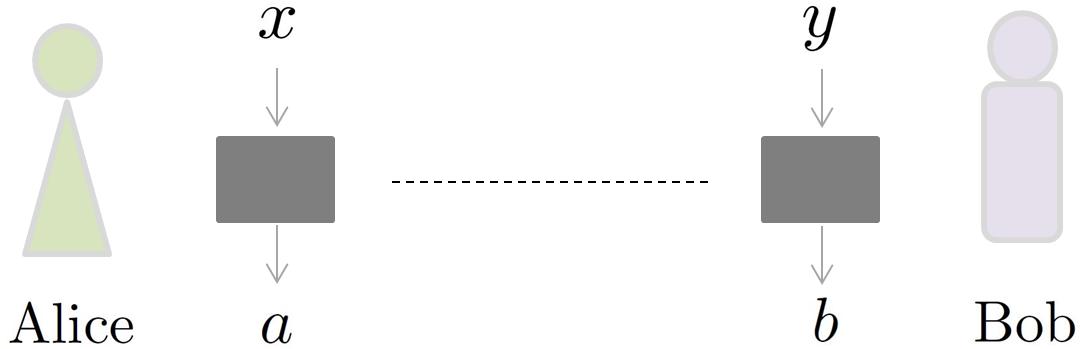
Figure 2: Representation of a XOR game. The goal is that Alice and Bob output $a$ and $b$ such that $a\oplus b=f(x,y)$.

In an XOR game, see Fig. 2, the referee provides queries $x\in[m_{A}]$ to one player (Alice) and $y\in[m_{B}]$ to the second player (Bob), with the promise that queries are sampled from some prior probability distribution $q(x,y)$ known to both players. In order to win the game, upon receiving their inputs $x$ and $y$, Alice and Bob must produce a binary output $a,b\in\{0,1\}$, respectively, such that $a\oplus b=f(x,y)$, where $f$ is a given Boolean function also known to both players. The performance of Alice and Bob’s strategy is quantified by the average winning probability

$$\omega=\sum_{x,y}q(x,y)p\!\left(a\oplus b\!=\!f(x,y)|x,y\right)=\frac{1}{2}(1+\xi),$$ (2)

where $\xi=\sum_{x,y}q(x,y)(-1)^{f(x,y)}c_{xy}$ is the gain (or bias). Note that XOR games can always be won with at least probability $\frac{1}{2}$ if Alice (or Bob) produces a random output independently of the input. Since $q(x,y)$ and $f(x,y)$ are a given, we can characterise the game by the so-called game matrix $\Phi=\sum_{x,y}(-1)^{f(x,y)}q(x,y)|x\rangle\!\langle y|,$ so that the gain can be written in terms of the correlation matrix as $\xi=\operatorname{tr}{C\Phi^{T}}$. Every correlation Bell inequality, as it is based on a linear function of the correlators $C$, can be written in the form $\operatorname{tr}{C\Phi^{T}}\leq\xi$, and by rescaling if necessary, $\Phi$ can be chosen as the game matrix of a suitable XOR game. The optimal classical success probability can always be attained by extremal (i.e. deterministic) strategies $|\alpha_{c}\rangle$ and $\left|\beta_{c}\right\rangle$, with $C=|\alpha_{c}\rangle\!\langle\beta_{c}|$. Hence the gain of the local classical average winning probability can be written as:

$$\xi_{c}=\max_{\alpha_{c},\beta_{c}}{\langle\alpha_{c}|}\Phi|\beta_{c}\rangle.$$ (3)

In the Supplementary Material (A) we present various useful ways to write the quantum gain, which are employed in the proofs of our main results.

It is easy to see that no-signalling behaviours allow to win XOR games with $\omega_{NS}=1$ ramanathan_characterizing_2014 , and therefore any XOR game with $\omega_{c}<1$ will correspond to a nontrivial Bell inequality, i.e. one that can potentially be violated quantumly. See the Supplementary Material (B) for further discussion of this point.

Observe finally that without loss of generality, we may restrict ourselves to XOR games with game matrices $\Phi$ that have no all-zero rows or columns. Indeed, because such a row or column of zeros imply that the marginal $q(x)$ or $q(y)$ are zero for some inputs, we can redefine the set of possible queries (decreasing $m_{A}$ or $m_{B}$ accordingly) to obtain an equivalent game without all-zero rows or columns in its game matrix. We refer to such games with $q(x)>0$ and $q(y)>0$ for all $x\in[m_{A}]$ and $y\in[m_{B}]$ as exhaustive games.

Results.— For a long time, it was implicitly assumed that if Alice and Bob use entangled strategies, they can attain a greater success probability than if they are limited to classical resources, for any nontrivial Bell inequality. As explained in the introduction, it took a while to find examples of nontrivial games that do not show any quantum advantage.

Here we show that XOR games (which characterise the correlation polytope) without quantum advantage never define a facet of the Bell polytope (full behaviours or correlations). This in turn implies that all (nontrivial) tight correlation Bell inequalities have quantum violations.

In ramanathan_characterizing_2014 Ramanathan et al. derived a necessary and sufficient condition for a two-player XOR game to have no quantum advantage, which will turn out to be fundamental for the proof of our first result.

Theorem 1.

If an exhaustive XOR game has no quantum advantage, the corresponding Bell inequality does not define a facet of the Bell polytope, nor of the correlation Bell polytope.

The proof – see the Supplementary Material (C) for full details – proceeds by bounding the dimension of the face $\mathcal{F}$ in the Bell polytope corresponding to the maximum classical bias $\xi_{c}$ of the given XOR game:

$$\begin{split}\mathcal{F}&=\{(\left|\alpha\right\rangle,\left|\beta\right\rangle,C)\in\mathcal{C}:\operatorname{tr}C\Phi^{T}=\xi_{c}\}\\ &=\operatorname{conv}\left\{(\left|\alpha_{c}\right\rangle,\left|\beta_{c}\right\rangle,\left|\alpha_{c}\rangle\!\langle\beta_{c}\right|):\left\langle\alpha_{c}\right|\Phi\left|\beta_{c}\right\rangle=\xi_{c}\right\}.\end{split}$$

The first ingredient is the characterisation of the maximum quantum bias $\xi_{Q}$ by semidefinite programming (SDP) Wehner , which by SDP duality leads to strong constraints on any optimal strategy via complementary slackness. From the assumption that $\xi_{Q}=\xi_{c}$, this leads to the second, and key, insight of the proof, namely that in any pair $(\left|\alpha_{c}\right\rangle,\left|\beta_{c}\right\rangle)$ of optimal classical strategies, Alice’s and Bob’s local answers uniquely determine each other linearly: as we show in the proof, $\left|\beta_{c}\right\rangle=F\left|\alpha_{c}\right\rangle$ for a certain matrix $F$. Assuming w.l.o.g. $m_{A}\leq m_{B}$, we thus have

$$\mathcal{F}=\operatorname{conv}\left\{(\left|\alpha_{c}\right\rangle\!,F\left|\alpha_{c}\right\rangle\!,\left|\alpha_{c}\right\rangle\!\!\left\langle\alpha_{c}\right|F^{T}):\left|\alpha_{c}\right\rangle\text{ opt.}\right\},$$

and its dimension can be upper bounded by that of

$$\operatorname{aff}\left\{(\left|\alpha_{c}\right\rangle\!,F\left|\alpha_{c}\right\rangle\!,\left|\alpha_{c}\right\rangle\!\!\left\langle\alpha_{c}\right|F^{T}):\left|\alpha_{c}\right\rangle\in\{\pm 1\}^{m_{A}}\right\},$$

which is $m_{A}+\frac{1}{2}m_{A}(m_{A}-1)<D-1$. In the case of the correlation polytope, the dimension is similarly upper bounded by $\frac{1}{2}m_{A}(m_{A}-1)<m_{A}m_{B}$.

Theorem 2.

All nontrivial tight correlation Bell inequalities for bipartite systems with binary outcomes have a quantum violation.

Proof.

Consider a (non-exhaustive) XOR game with $M_{A}$ (Alice) and $M_{B}$ (Bob) inputs. W.l.o.g. the first $m_{A}$ ($m_{B}$) inputs of Alice (Bob) have non-zero probability, the rest are never asked, so we can apply Theorem 1 to the reduced exhaustive game, which relates the optimal strategies for the indices $x\in[m_{A}]$ and $y\in[m_{B}]$, but leaves completely unconstrained the remaining ones. Hence, given a strategy by Alice $|\alpha_{c}\rangle\oplus|\alpha_{c}^{\prime}\rangle$, Bob’s strategy must be $(F|\alpha_{c}\rangle)\oplus|\beta_{c}^{\prime}\rangle$, where $|\alpha_{c}^{\prime}\rangle\in\{\pm 1\}^{M_{A}-m_{A}}$ and $|\beta_{c}^{\prime}\rangle\in\{\pm 1\}^{M_{B}-m_{B}}$.

We thus arrive at a codimension $\Delta=D-\dim\mathcal{F}$ of the face of $\Delta\geq m_{B}+M_{A}(m_{B}-m_{A})+\frac{m_{A}}{2}(m_{A}+1)>1$. That is, XOR games with quantum equal to classical value do not define a facet of the full Bell polytope. Following the same argument for the correlation polytope leads to the codimension $\Delta_{0}\geq M_{A}(m_{B}-m_{A})+\frac{1}{2}m_{A}(m_{A}+1)$, and this is greater than $1$ unless $m_{A}=m_{B}=1$, corresponding precisely to the trivial inequalities $|c_{xy}|\leq 1$. ∎

In the Supplementary Material (D) we give a different proof of the above result for non-local computation games, showing also that the dimension bounds are asymptotically attained for nontrivial games.

From the proof of Theorem 1 we learn that the optimal extremal behaviours in an exhaustive XOR game with no quantum advantage are fully determined by the strategy of one of the parties. We will now show that this feature actually extends to all optimal quantum behaviours of arbitrary XOR games.

To understand the following theorem, we recall the definition of a face $\mathcal{F}\subset\mathcal{Q}$ of a general compact convex set $\mathcal{Q}$: namely, that whenever $\mathcal{F}\ni\vec{p}=t\vec{q}+(1-t)\vec{r}$, $0<t<1$, then both $\vec{q},\,\vec{r}\in\mathcal{F}$. An exposed face is obtained as $\mathcal{F}=\mathcal{Q}\cap H$ with a supporting hyperplane $H$ of $\mathcal{Q}$; all exposed faces are faces of $\mathcal{Q}$, but not vice versa. However, for polytopes every face is an exposed face Rockafeller ; ConvexPolytopes . Also, facets, and more generally maximal faces, are always exposed.

Note that this result explains the previous two theorems on the classical behaviours as being due to broader properties of the quantum sets.

Theorem 3.

Nontrivial XOR games, or equivalently nontrivial correlation Bell inequalities, never define a facet of the quantum sets of behaviours $\mathcal{Q}_{\text{com}}$ and $\mathcal{Q}_{\otimes}$. As a consequence, the set $\mathcal{Q}_{0}$ of quantum correlations has no nontrivial facets.

See the Supplementary Material (C) for the complete proof. To give the broad outline, we start with an exhaustive XOR game. The complementary slackness condition in the proof of Theorem 1 for the optimal quantum strategy leads to $|\beta_{y}\rangle=\sum_{x^{\prime}}F_{yx^{\prime}}|\alpha_{x^{\prime}}\rangle$, with the same matrix $F$ as before. In other words, once again Alice’s optimal quantum strategy uniquely determines Bob’s, and vice versa.

Thus, we get for an optimal quantum correlation matrix $C_{xy}=\left\langle\alpha_{x}\lvert\beta_{y}\right\rangle=\sum_{x^{\prime}}F_{yx^{\prime}}\left\langle\alpha_{x}\lvert\alpha_{x^{\prime}}\right\rangle$, and hence the dimension of their affine span is bounded by that of the Gram matrices $[\left\langle\alpha_{x}\lvert\alpha_{x^{\prime}}\right\rangle]_{xx^{\prime}}$, with dimension $\frac{1}{2}m_{A}(m_{A}-1)$, leading to the same dimension bound as in the proof of Theorem 1. Non-exhaustive XOR games are treated as in the proof of Theorem 2.

Discussion and outlook.— We have shown that a two-party correlation Bell inequality (XOR game) with no quantum violation (quantum advantage) cannot define a facet of the Bell polytope. The contrapositive of this statement has deep physical implications: all tight correlation Bell inequalities exhibit a quantum violation. In fact, we have proven lower bounds on the codimension of the defined face (increasing with the number of inputs). As a consequence, when the codimension is lower bounded by $\Delta>1$, not only all tight correlation inequalities will have quantum violations, but also those corresponding to faces $\mathcal{F}$ with $\dim\mathcal{F}\geq D-\Delta$.

On the way, we have proved that this in fact is due to a broader property of the convex set of quantum correlations, namely that it does not have any non-trivial facets, only lower-dimensional faces. It remains to be seen what the physical meaning of this curious geometric observation is.

Our results appear very much tied to the world of two-player, binary outcome XOR games. This leaves open the questions whether XOR games for more than two players can define common facets of the quantum and classical sets (note that GYNI defines such a facet, but it is not an XOR game), and whether for two players there are any tight Bell inequalities at all without quantum violations. It might be possible to extend our results at least two two-players MOD-$q$ games where each player has a $q$-ary outcome.

Acknowledgements.— We thank Mafalda Almeida, Nicolas Brunner and Paul Skrzypczyk for discussions on non-local computation, and Dardo Goyeneche for rekindling our interest in Bell inequalities without quantum violation. Support from the Spanish MINECO, project FIS2016-80681-P with the support of AEI/FEDER funds, and from the Generalitat de Catalunya, project CIRIT 2017-SGR-1127, is acknowledged.

I Supplementary Material

I.1 A. Quantum bias

If Alice and Bob use quantum resources, i.e. a (possibly) entangled state $|\psi\rangle\in\mathcal{H}$, with with observables $\hat{a}_{x}$ and $\hat{b}_{y}$ depending on their respective inputs $x$ and $y$, to produce their measurement outcomes $a$ and $b$, then, using the expression given in the main text for the quantum correlations $c_{xy}$, the quantum gain can be written as

$$\begin{split}\xi_{Q}&=\sum_{x,y}q(x,y)\left\langle\psi\right|(-1)^{\hat{a}_{x}+\hat{b}_{y}+f(x,y)}\left|\psi\right\rangle\\ &=\sum_{x,y}q(x,y)(-1)^{f(x,y)}\left\langle\alpha_{x}\right|\beta_{y}\rangle,\end{split}$$ (4)

with $\left|\alpha_{x}\right\rangle=(-1)^{\hat{a}_{x}}\left|\psi\right\rangle$ and $\left|\beta_{y}\right\rangle=(-1)^{\hat{b}_{y}}\left|\psi\right\rangle$ unit vectors in $\mathcal{H}$. Vice versa, given any set of unit vectors in any complex Hilbert space, there exists an equivalent set, i.e. with the same pairwise inner products $\left\langle\alpha_{x}\right|\beta_{y}\rangle$, of the above form, on a tensor product Hilbert space [12]. It will prove convenient to define the following states on an extended vector space,

$$\begin{split}|\alpha\rangle_{Q}&=\sum_{x}(-1)^{\hat{a}_{x}}\left|\psi\right\rangle\otimes\left|x\right\rangle,\\ |\beta\rangle_{Q}&=\sum_{y}(-1)^{\hat{b}_{y}}\left|\psi\right\rangle\otimes\left|y\right\rangle.\end{split}$$ (5)

With this, the expression for the optimal quantum gain reads

$$\xi_{Q}=\max_{\left|\alpha\right\rangle_{Q},\left|\beta\right\rangle_{Q}}{{}_{Q}\langle\alpha|}\mathbb{I}\otimes\Phi|\beta\rangle_{Q},$$ (6)

which resembles the expression (3) for its classical counterpart.

I.2 B. XOR games can always be won using no-signalling behaviours

It is easy to understand the previous observation of $\omega_{NS}=1$ for every XOR game, by realising that an XOR game can always be won with certainty using a behaviour that outputs uniformly random local bits $a$ and $b$, and so is evidently no-signalling:

$$p(a,b|x,y)=\begin{cases}\frac{1}{2}&\text{ if }a\oplus b=f(x,y),\\ 0&\text{ otherwise}.\end{cases}$$ (7)

This behaviour has $\left|\alpha\right\rangle=\left|\beta\right\rangle=0$, but its correlator term is remarkably $c_{xy}=(-1)^{f(x,y)}$, i.e. an arbitrary $\pm 1$-matrix. In geometric terms, this says that $\mathcal{NS}_{0}$ is the $\ell_{\infty}$ unit ball (aka hypercube), in other words $\mathcal{NS}_{0}$ is entirely characterised by the inequalities $-1\leq c_{xy}\leq 1$. These are indeed the trivial Bell inequalities, since they follow from the non-negativity of the probabilities $p(a,b|x,y)$.

To back up the definite article in the previous statement, it is in fact known that they not only define facets of $\mathcal{NS}_{0}$, but also of $\mathcal{C}_{0}$ and thus of $\mathcal{Q}_{0}$; namely, for every pair $(x_{0},y_{0})$, the behaviour $C_{0}=\left|x_{0}\rangle\!\langle y_{0}\right|$ is in $\mathcal{C}_{0}$, and so is an entire sufficiently small neighbourhood of $C_{0}$ of correlators $C$ in the supporting hyperplane $H=\{C:C_{x_{0}y_{0}}=1\}$ (and analogously for $-C_{0}$). Again, this is easy to see: consider local classical strategies $\left|\alpha_{c}\right\rangle=\sum_{x}\alpha_{x}\left|x\right\rangle$ and $\left|\beta_{c}\right\rangle=\sum_{y}\beta_{y}\left|y\right\rangle$ with $\alpha_{x_{0}}=\beta_{y_{0}}=1$, so that we can write $\left|\alpha_{c}\right\rangle=\left|x_{0}\right\rangle+\left|\alpha^{\prime}\right\rangle$ and $\left|\beta_{c}\right\rangle=\left|y_{0}\right\rangle+\left|\beta^{\prime}\right\rangle$. Then,

$$\left|\alpha_{c}\rangle\!\langle\beta_{c}\right|=C_{0}+\left|x_{0}\rangle\!\langle\beta^{\prime}\right|+\left|\alpha^{\prime}\rangle\!\langle y_{0}\right|+\left|\alpha^{\prime}\rangle\!\langle\beta^{\prime}\right|.$$ (8)

By taking convex combinations over $\left|\beta^{\prime}\right\rangle=\epsilon\left|y_{1}\right\rangle+\sum_{y\neq y_{0},y_{1}}\beta_{y}\left|y\right\rangle$, with uniformly random $\beta_{y}=\pm 1$ ($y\neq y_{0},y_{1}$) and uniformly random $\left|\alpha^{\prime}\right\rangle$, we annihilate all terms except one, showing that $C_{0}+\epsilon\left|x_{0}\rangle\!\langle y_{1}\right|\in\mathcal{C}_{0}$, for $\epsilon=\pm 1$. Similarly, we find $C_{0}+\epsilon\left|x_{1}\rangle\!\langle y_{0}\right|\in\mathcal{C}_{0}$. Finally, by taking convex combinations over $\left|\alpha^{\prime}\right\rangle=\sum_{x\neq x_{0}}\alpha_{x}\left|x\right\rangle$ and $\left|\beta^{\prime}\right\rangle=\epsilon\alpha_{x_{1}}\left|y_{1}\right\rangle+\sum_{y\neq y_{0},y_{1}}\beta_{y}\left|y\right\rangle$, with uniformly random $\left|\alpha^{\prime}\right\rangle$ and uniformly random $\beta_{y}=\pm 1$ ($y\neq y_{0},y_{1}$), we get that $C_{0}+\epsilon\left|x_{1}\rangle\!\langle y_{1}\right|\in\mathcal{C}_{0}$. The convex hull of all these points, a hyper-octahedron, contains a small neighbourhood of $C_{0}$ in the hyperplane $H$.

I.3 C. Proofs

Here, we give the complete proofs of Theorems 1 and 3 in the main text.

Proof of Theorem 1.  Our aim is to bound the dimension of the face $\mathcal{F}$ defined by the maximum classical bias $\xi$ of a given XOR game:

$$\begin{split}\mathcal{F}&=\{(\left|\alpha\right\rangle\!,\left|\beta\right\rangle\!,C)\in\mathcal{C}:\operatorname{tr}C\Phi^{T}=\xi_{c}\}\\ &=\operatorname{conv}\left\{(\left|\alpha_{c}\right\rangle\!,\left|\beta_{c}\right\rangle\!,\left|\alpha_{c}\rangle\!\langle\beta_{c}\right|):\left\langle\alpha_{c}\right|\Phi\left|\beta_{c}\right\rangle=\xi_{c}\right\}.\end{split}$$ (9)

In particular, we want to show that its dimension $\dim\mathcal{F}$ is strictly lower than the dimension of a facet, $D-1$, or equivalently that the codimension of the face in the classical polytope is $\Delta=D-\dim\mathcal{F}>1$.

We start by considering the consequences of assuming no quantum advantage, i.e. $\xi_{c}=\xi_{Q}$. The optimal quantum gain can be written as $\xi_{Q}=\max_{C}\operatorname{tr}{C\Phi^{T}}$, where $C=\sum_{x,y}\langle\alpha_{x}|\beta_{y}\rangle\left|x\rangle\!\langle y\right|$ is the quantum correlator matrix, which is fully characterised [12] by the inner products of an arbitrary set of unit vectors in ${\mathbb{R}}^{m_{A}+m_{B}}$. In terms of the characterisation in (5), $\left|\alpha_{x}\right\rangle=\left\langle x\lvert\alpha\right\rangle_{Q}=(-1)^{\hat{a}_{x}}|\psi\rangle$, and analogously for Bob’s strategy. In order to write this optimisation problem as a semidefinite program [18, 37] we define the following Gram matrix

$$\tilde{Q}=\left(\begin{array}[]{c|c}R&C\\ \hline\cr C^{T}&S\\ \end{array}\right),$$ (10)

with $R_{xx^{\prime}}=\langle\alpha_{x}|\alpha_{x^{\prime}}\rangle$ and $S_{yy^{\prime}}=\langle\beta_{y}|\beta_{y^{\prime}}\rangle$. An equivalent characterisation of a Gram matrix of unit vectors is $\tilde{Q}\succeq 0$ and $\tilde{Q}_{ii}=1$ for all $i\in[m_{A}+m_{B}]$, and consequently we can write the maximum quantum gain as:

$$\begin{split}\xi_{Q}&=\max_{\tilde{Q}}\operatorname{tr}{\tilde{Q}\tilde{\Phi}},\\ &\text{ s.t. }\operatorname{diag}(\tilde{Q})=(1,..,1),\,\tilde{Q}\succeq 0,\end{split}$$ (11)

where $\tilde{\Phi}=\frac{1}{2}\left(\begin{array}[]{c|c}0&\Phi\\ \hline\cr\Phi^{T}&0\\ \end{array}\right)$.

Consider now the Lagrangian,

$$\begin{split}L&=\operatorname{tr}{\tilde{Q}\tilde{\Phi}}-\sum_{i}t_{i}\left(\operatorname{tr}{|i\rangle\!\langle i|\tilde{Q}}-1\right)\\ &=\operatorname{tr}\left[\tilde{Q}(\tilde{\Phi}-\sum_{i}t_{i}|i\rangle\!\langle i|)\right]+\sum_{i}t_{i},\end{split}$$ (12)

where $t_{i}\in{\mathbb{R}}$ are the Lagrange multipliers. Therefore,

$$\max_{\tilde{Q}\succeq 0}L=\begin{cases}+\infty&\text{ if }\sum_{i}t_{i}|i\rangle\!\langle i|-\tilde{\Phi}\not\succeq 0,\\ \sum_{i}t_{i}&\text{ if }\sum_{i}t_{i}|i\rangle\!\langle i|-\tilde{\Phi}\succeq 0,\end{cases}$$ (13)

and thus the original SDP (11) can be written in its dual form,

$$\min\sum_{i}t_{i}\text{ s.t.}\sum_{i}t_{i}|i\rangle\!\langle i|\succeq\tilde{\Phi}.$$ (14)

This holds because the primal and dual SDPs satisfy the condition for strong duality.

From the above construction it follows that $\operatorname{tr}{\tilde{Q}\tilde{\Phi}}\leq\xi_{Q}\leq\sum_{i}t_{i}$ for any pair of primal and dual feasible solutions. Furthermore, by strong duality, the maximum primal value $\xi_{Q}$ equals the solution of the dual (14). That is, the optimal value is attained if and only if $\operatorname{tr}{\tilde{Q}\tilde{\Phi}}=\sum_{i}t_{i}$, or equivalently if the spurious term in the Lagrangian vanishes: $\operatorname{tr}\left[\tilde{Q}\left(\sum_{i}t_{i}|i\rangle\langle i|-\tilde{\Phi}\right)\right]=0$ (complementary slackness). Note that by the form of the dual problem (14), the $t_{i}$ are non-negative numbers; indeed, by our assumption that $\Phi$ has no all-zero rows or columns, we even can conclude that all $t_{i}>0$.

Now, our hypothesis of no quantum advantage implies that $\xi_{Q}$ coincides with its classical counterpart $\xi_{c}={\langle}\beta_{c}|\Phi|\alpha_{c}\rangle=\operatorname{tr}\left|s\rangle\!\langle s\right|\tilde{\Phi}^{T}$, where we have defined $|s\rangle=|\alpha_{c}\rangle\oplus|\beta_{c}\rangle$. In other words, $\xi_{Q}$ can be reached with a classical correlation matrix $\tilde{Q}=\left|s\rangle\!\langle s\right|$. Letting $\Gamma=\sum_{i}t_{i}|i\rangle\!\langle i|=\frac{1}{2}\Sigma\oplus\Lambda\succ 0$, where $\Sigma$ and $\Lambda$ are diagonal positive definite matrices, the slackness condition reads $\operatorname{tr}\left[(\Gamma-\tilde{\Phi})\left|s\rangle\!\langle s\right|\right]=0$, which in turn implies that $(\Gamma-\tilde{\Phi})\left|s\right\rangle=0$, since both $\Gamma-\tilde{\Phi}$ and $\left|s\rangle\!\langle s\right|$ are positive semidefinite. Therefore, $\Sigma|\alpha_{c}\rangle=\Phi|\beta_{c}\rangle$ and $\Lambda|\beta_{c}\rangle=\Phi^{T}|\alpha_{c}\rangle$, or equivalently

$$|\alpha_{c}\rangle=\Sigma^{-1}\Phi|\beta_{c}\rangle,\,|\beta_{c}\rangle=\Lambda^{-1}\Phi^{T}|\alpha_{c}\rangle=:F|\alpha_{c}\rangle.$$ (15)

This means that once Alice’s optimal strategy is fixed, Bob’s best strategy is uniquely determined by her choice and vice versa. Assuming w.l.o.g. $m_{A}\leq m_{B}$, the dimension of the face $\mathcal{F}$ generated by such strategies is then

$$\dim\mathcal{F} =\dim\operatorname{aff}\left\{(\left|\alpha_{c}\right\rangle\!,F\left|\alpha_{c}\right\rangle\!,\left|\alpha_{c}\right\rangle\!\!\left\langle\alpha_{c}\right|F^{T}):\left|\alpha_{c}\right\rangle\text{ opt.}\right\}$$

$$\leq\dim\operatorname{aff}\left\{(\left|\alpha_{c}\right\rangle\!,\left|\alpha_{c}\right\rangle\!,\left|\alpha_{c}\right\rangle\!\!\left\langle\alpha_{c}\right|):\left|\alpha_{c}\right\rangle\in\{\pm 1\}^{m_{A}}\right\}$$

$$=m_{A}+\frac{m_{A}(m_{A}-1)}{2},$$ (16)

where $\operatorname{aff}$ denotes the affine span, and where the second term in the dimension comes from the fact that the affine span of the matrices $\left|\alpha_{c}\right\rangle\!\left\langle\alpha_{c}\right|$ consists precisely of the real symmetric matrices with $1$’s along the diagonal. This leads to a codimension of the face in the Bell polytope of $\Delta\geq m_{B}+m_{A}m_{B}-\frac{1}{2}m_{A}(m_{A}-1)>1$.

Similarly, we can bound the codimension of this facet in the correlation polytope, which is solely generated by the correlators $\left|\alpha_{c}\right\rangle\!\left\langle\alpha_{c}\right|F^{T}$, leading to $\Delta_{0}\geq m_{A}m_{B}-\frac{1}{2}m_{A}(m_{A}-1)>1$, unless $m_{A}=m_{B}=1$, which is a trivial case.

Therefore, we see that the defined face is not a facet in either setting. ∎

Proof of Theorem 3.  Starting from the definition $|q\rangle=|\alpha\rangle_{Q}\oplus|\beta\rangle_{Q}$, we can write the quantum bias as $\xi_{Q}={{}_{Q}\!{\langle}}\beta|\Phi|\alpha\rangle_{Q}=\langle q|\openone\otimes\tilde{\Phi}|q\rangle$. It is straightforward to check, following the steps in the proof of Theorem 1, that the complementary slackness condition translates into $(\openone\otimes\Gamma-\openone\otimes\tilde{\Phi})\left|q\right\rangle=0$, which in the case of exhaustive games leads to

$$|\beta\rangle_{Q}=(\openone\otimes F)|\alpha\rangle_{Q},$$ (17)

or equivalently $|\beta_{y}\rangle=\sum_{x^{\prime}}F_{yx^{\prime}}|\alpha_{x^{\prime}}\rangle$, with the same matrix $F$ as in the proof of Theorem 1. This shows that Bob’s optimal quantum strategy (as encoded in the vectors $\{\left|\beta_{y}\right\rangle\}$) is fully determined by Alice optimal strategy (the vectors $\{\left|\alpha_{x}\right\rangle\}$).

In order to bound the dimensionality of the behaviours that determine the corresponding face we note that $c_{xy}=\left\langle\alpha_{x}\lvert\beta_{y}\right\rangle=\sum_{x^{\prime}}F_{yx^{\prime}}\left\langle\alpha_{x}\lvert\alpha_{x^{\prime}}\right\rangle$. The dimension of the affine span of the optimal behaviours $C$ is clearly bounded by that of the Gram matrices $[\left\langle\alpha_{x}\lvert\alpha_{x^{\prime}}\right\rangle]_{xx^{\prime}}$, which we recall to be real symmetric matrices with diagonal elements $\left\langle\alpha_{x}\lvert\alpha_{x}\right\rangle=1$, thus the dimension is bounded by $\frac{1}{2}m_{A}(m_{A}-1)$ and therefore the codimension of the face of $\mathcal{Q}_{0}$ is bounded by the classical bound derived in Theorem 1. To get the same for $\mathcal{Q}_{\text{com}}$ and $\mathcal{Q}_{\otimes}$, we need to control also the marginal parts of the behaviours, which can be written as $\alpha_{x}=\left\langle\psi\lvert\alpha_{x}\right\rangle$ and $\beta_{y}=\left\langle\psi\lvert\beta_{y}\right\rangle=\sum_{x^{\prime}}F_{yx^{\prime}}\alpha_{x^{\prime}}$. In other words, $\left|\beta\right\rangle=F\left|\alpha\right\rangle$ is fully determined by $\left|\alpha\right\rangle$, just as we had seen for the deterministic classical strategies, hence only $m_{A}$ is added to the dimension of the face.

For non-exhaustive XOR games we then proceed as in Theorem 2. In particular, XOR games do not define facets of either $\mathcal{Q}_{\text{com}}$ or $\mathcal{Q}_{\otimes}$. In the quantum correlation set $\mathcal{Q}_{0}$, the XOR games that can define facets have only one input each for Alice and Bob, and that leaves only $|c_{xy}|\leq 1$, which are indeed facet defining inequalities, but they are trivial, as they correspond to the non-negativity of probability.

To arrive at the conclusion for $\mathcal{Q}_{0}$ having no facets at all, note that any purported facet is exposed, so it has to be defined by an XOR game, and for those we just showed that only the trivial inequalities define facets. ∎

I.4 D. Dimension bound for non-local computation and (asymptotic) attainability

In [21], Linden et al. introduced the cooperative games of non-local computation (NLC) and showed that quantum strategies provide no advantage over classical ones, although stronger forms of non-signaling correlations allowed perfect success. In the problem of non-local computation Alice and Bob need to collaborate in order to compute to a boolean function $f(z)$ of a string of $n$ bits, $z=z_{1}z_{2}\ldots z_{n}$, without communicating with each other during the computation, and without individually learning anything about the input string $z$. The inputs are promised to be given with an arbitrary probability distribution $\tilde{q}(z)$ known to Alice and Bob and are split in two correlated signals $x=x_{1}x_{2}\ldots x_{n}$ and $y=y_{1}y_{2}\ldots y_{n}$ so that $z=x\oplus y$ (meaning $x_{i}\oplus y_{i}=z_{i}$ for all $i=1,\ldots,n$) which are given to Alice and Bob respectively. In order to enforce that Alice and Bob do not learn anything about $z$, it is necessary that $p(x_{i}=0)=p(x_{i}=1)=\frac{1}{2}$ for all $x_{i}$ and idem for $y_{i}$. It is hence clear that NLC is a particular instance of an XOR game with $q(x,y)=\frac{1}{2^{n}}\tilde{q}(x\oplus y)$ and $a\oplus b=f(z=x\oplus y)$.The corresponding game matrix is given by $\Phi_{NLC}=\sum_{x,y}(-1)^{f(x\oplus y)}\tilde{q}(x\oplus y)|x\rangle\!\langle y|$.

In [21], it is proved that the game matrix is diagonal in the Fourier (Hadamard) basis, $|\tilde{u}\rangle=\sum_{x}(-1)^{u\cdot x}|x\rangle$, where $u\cdot x$ is the inner product modulo $2$ of the bit strings $u$ and $x$. As a consequence, $\xi_{Q}\leq 2^{n-1}\|\Phi_{NLC}\|:=\xi^{*}$, where $\|\cdot\|$ denotes the operator norm. Moreover, it was shown that the upper bound is attained by a classical local strategy with $\xi_{c}=\xi^{*}$, i.e. by a suitably chosen pair of vectors $\left|\alpha_{c}\right\rangle$, $\left|\beta_{c}\right\rangle$, and one concludes that NLC games present no quantum advantage. Since the inequality

$$\xi\leq\xi^{*}$$ (18)

holds for any classical local and quantum average success probability, this Bell inequality is neither violated by classical physics nor quantum mechanics and thus we have that the Bell polytope and the quantum set share a region of their boundary.

The result stated below as Corollary 4 (because it follows from Theorem 1) was first proved in [25]. It says that an NLC Bell inequality is never tight for any number of inputs. Here we present an alternative proof, based on directly bounding the dimension of the face defined by the Bell inequality. This is a reconstruction of the earlier unpublished proof referenced in [24].

Corollary 4.

For any number $n$ of input bits, an NLC game never defines a facet of the Bell polytope, nor of the correlation polytope.

Proof.

As $m_{A}=m_{B}=2^{n}$, the dimension of the Bell polytope is $D=4^{n}+2^{n+1}$. In order to see that the NLC Bell inequality does not define a facet, we show that the dimension of the affine space generated by the optimal classical strategies is strictly smaller than $D-1$. The local classical success probability is bounded by $\omega^{*}=\frac{1}{2}(1+\xi^{*})$, which only depends on $\lambda=\|\Phi_{NLC}\|$. Let $|u_{0}\rangle$ be a corresponding eigenvector of $\pm\lambda$.

Now, $\xi$ achieves the maximum value when $|\alpha_{c}\rangle$ and $|\beta_{c}\rangle$ are both proportional to $|u_{0}\rangle$, i.e. $|\alpha_{c}\rangle=\pm|\beta_{c}\rangle=\pm|u_{0}\rangle$. Thus, we consider the eigenspaces of the two eigenvalues $\pm\lambda$, which we denote by $\text{Eig}(\lambda)$ and $\text{Eig}(-\lambda)$, respectively. There are two cases: either $|\alpha_{c}\rangle=|\beta_{c}\rangle\in\text{Eig}(\lambda)$ or $|\alpha_{c}\rangle=-|\beta_{c}\rangle\in\text{Eig}(-\lambda)$. These we can write in a single equation as $\left|\beta_{c}\right\rangle=F\left|\alpha_{c}\right\rangle$, with $F=2\Pi_{\lambda}-\openone$ and $\Pi_{\lambda}$ the projector onto the eigenspace $\text{Eig}(\lambda)$.

Therefore, the face $\mathcal{F}_{NLC}$ that these optimal strategies define, is contained in the following affine subspace:

$$\begin{split}\operatorname{aff}&\left\{(\left|\alpha_{c}\right\rangle\!,F\left|\alpha_{c}\right\rangle\!,\left|\alpha_{c}\rangle\!\langle\alpha_{c}\right|F):\left|\alpha_{c}\right\rangle\in\{\pm 1\}^{2^{n}}\right\},\end{split}$$ (19)

whose dimension we have already bounded before, in the proof of Theorem 1, Eq. (I.3), and so

$$\dim\mathcal{F}_{NLC}\leq 2^{n}+{2^{n-1}(2^{n}-1)},$$ (20)

and codimension $\Delta\geq 2^{n}+{2^{n-1}(2^{n}+1)}>1$.

For the correlation polytope, we get similarly that the dimension of the face is upper bounded by ${2^{n-1}(2^{n}-1)}$, resulting in a bound of $\Delta_{C}\geq{2^{n-1}(2^{n}+1)}>1$ for the codimension of the face.

The bound Eq. (20) is achievable with equality for $\Phi=2^{-n}\openone$; this describes a game where $x$ is uniformly distributed, and $y=x$, and to win, Alice and Bob have to output the same bit $a=b$. This is evidently possible with probability $1$, using any local strategy $\left|\alpha_{c}\right\rangle$ for Alice and $\left|\beta_{c}\right\rangle=\left|\alpha_{c}\right\rangle$ for Bob, i.e. $\alpha_{x}=\beta_{x}$ for all $x\in\{0,1\}^{n}$, so that $F=\openone$ above. Thus, the resulting face attains Eq. (20) with equality; likewise, the corresponding face in the correlation polytope has dimension $\dim\mathcal{F}_{C}={2^{n-1}(2^{n}-1)}$. Of course, one might object that this game has winning probability $\omega_{c}=1$, equal to the no-signalling bound, so in some sense it is trivial, but it is worth noting that the Bell inequality is not a trivial one ($|c_{xy}|\leq 1$). ∎

We can get a slightly better bound, sometimes much better depending on the game matrix $\Phi$, by exploiting the fact that the latter is Hermitian and that the optimal local strategies must lie either in $\text{Eig}(\lambda)$ or in $\text{Eig}(-\lambda)$; denote their dimensions by $k$ and $\ell$, respectively, so that $k+\ell\leq 2^{n}$. In the following we can discard the extreme cases $k=2^{n}$ and $\ell=2^{n}$, since those correspond to $\Phi\propto\openone$, which we have just discussed.

From the previous analysis, we have

$$\mathcal{F}_{NLC} =\operatorname{conv}\Bigl{\{}(\left|\alpha_{c}\right\rangle\!,\epsilon\left|\alpha_{c}\right\rangle\!,\epsilon\left|\alpha_{c}\rangle\!\langle\alpha_{c}\right|):\epsilon=\pm 1,\Bigr{.}$$

$$\phantom{=======:}\Bigl{.}\left|\alpha_{c}\right\rangle\in\text{Eig}(\epsilon\lambda)\cap\{\pm 1\}^{2^{n}}\Bigr{\}}$$ (21)

$$\subset\operatorname{span}\Bigl{\{}(\left|\alpha\right\rangle\!,\epsilon\left|\alpha\right\rangle\!,\epsilon\left|\alpha\rangle\!\langle\alpha\right|):\epsilon=\pm 1,\Bigr{.}$$

$$\phantom{=============:}\Bigl{.}\left|\alpha\right\rangle\in\text{Eig}(\epsilon\lambda)\Bigr{\}}$$ (22)

$$\!\!\!\!\!\!\!\!\!\!\!\!\!\!=\operatorname{span}\Bigl{\{}(\left|\alpha\right\rangle\!,-\left|\alpha\right\rangle\!,-\left|\alpha\rangle\!\langle\alpha\right|):\left|\alpha\right\rangle\in\text{Eig}(-\lambda)\Bigr{\}}$$

$$\!\!\!\!\!\!\!\oplus\operatorname{span}\Bigl{\{}(\left|\alpha\right\rangle\!,\left|\alpha\right\rangle\!,\left|\alpha\rangle\!\langle\alpha\right|):\left|\alpha\right\rangle\in\text{Eig}(\lambda)\Bigr{\}}.$$ (23)

Note that the linear span, in Eq. (22), denote it $\mathcal{L}$, has a dimension at least $1$ larger than the face $\mathcal{F}_{NLC}$, because the affine span of the latter does not contain the origin. This is due to the fact that otherwise the optimal classical winning probability were $\frac{1}{2}$, corresponding to a bias $0$, but it is easily seen that XOR game always have some positive bias [22].

Now, the spaces in Eq. (23) have dimension $\ell+\frac{1}{2}\ell(\ell+1)$ and $k+\frac{1}{2}k(k+1)$, respectively, and so

$$\begin{split}\dim\mathcal{F}_{NLC}&\leq\dim\mathcal{L}-1\\ &=k+\ell+\frac{k(k+1)}{2}+\frac{\ell(\ell+1)}{2}-1.\end{split}$$ (24)

Among the pairs with $k+\ell\leq 2^{n}$, and – as explained before – excluding $\Phi\propto\openone$, i.e. imposing $k,\ell<2^{n}$, the r.h.s. is maximised at $k=2^{n}-1$, $\ell=1$, for which values it reproduces the previously obtained bound $2^{n}+2^{n-1}(2^{n}-1)$. Note that this restricts the game severely, since the game matrix has only the two possible eigenvalues $\pm\lambda$, w.l.o.g. with multiplicities $2^{n}-1$ and $1$, respectively: this means $\Phi=\lambda F=\lambda(2\Pi_{\lambda}-\openone)$ and $\openone-\Pi_{\lambda}$ has rank $1$. In all other cases, Eq. (24) is strictly better than the bound (20). For the correlation polytope, we get similarly that the dimension of the face is upper bounded by $\frac{k(k+1)}{2}+\frac{\ell(\ell+1)}{2}-1\leq 2^{n-1}(2^{n}-1)$.

These bounds can be attained, if not exactly, then asymptotically, as we will show on the example $k=2^{n}-1$, $\ell=1$. By the analysis of [24], this essentially leaves only the game matrix $\Phi=\lambda(\openone-2^{-n}J)-\lambda 2^{-n}J$, where $J=\left|\bar{1}\rangle\!\langle\bar{1}\right|$ is the all-one-matrix, and $\left|\bar{1}\right\rangle=\sum_{x=1}^{2^{n}}\left|x\right\rangle.$ Since the sum of the absolute values of the entries of $\Phi$ has be to $1$, this fixes the value of $\lambda=\frac{1}{3\cdot 2^{n}-4}$, corresponding to the winning probability (classical and quantum) $\omega^{*}=\frac{1}{2}\left(1+\frac{2^{n}}{3\cdot 2^{n}-4}\right)\approx\frac{2}{3}<1$ for $n\geq 2$. I.e. the game, and with it its Bell inequality, is nontrivial. The game can be described as follows: $x$ and $y$ are jointly distributed according to $q(x,y)>0$, and to win, Alice and Bob have to output the same bit $a=b$ if $x=y$, and different bits $a\neq b$ if $x\neq y$. The optimal classical local strategies are on the one hand $\left|\alpha_{c}\right\rangle=\left|\bar{1}\right\rangle=-\left|\beta_{c}\right\rangle$ (corresponding to the single negative eigenvalue $-\lambda$ of $\Phi$), and $\left|\alpha_{c}\right\rangle=\left|\beta_{c}\right\rangle\perp\left|\bar{1}\right\rangle$ (corresponding to the $(2^{n}-1)$-fold eigenvalue $\lambda$). The latter means that $\left|\alpha_{c}\right\rangle=\left|\beta_{c}\right\rangle$ has to have exactly $2^{n-1}$ entries $+1$ and $2^{n-1}$ entries $-1$, of which there are ${2^{n}\choose 2^{n-1}}$. With this, we determine the dimension of the corresponding face of the correlation Bell polytope as

$$\dim\mathcal{F}=1+\dim\operatorname{aff}\left\{\left|\alpha_{c}\rangle\!\langle\alpha_{c}\right|:\left|\alpha_{c}\right\rangle\perp(\left|0\right\rangle+\left|1\right\rangle)^{\otimes n}\right\},$$

where it is understood that $\left|\alpha_{c}\right\rangle\in\{\pm 1\}^{2^{n}}$. The affine span on the r.h.s. is precisely the space $\mathcal{G}_{0}$ of real symmetric matrices with $1$’s along the diagonal and with the property that all row and column sums are $0$. By parameter counting, it is straightforward to see that $\dim\mathcal{G}_{0}=2^{n-1}(2^{n}-3)$, and so we get $\dim\mathcal{F}=1+2^{n-1}(2^{n}-3)\sim 2^{n-1}(2^{n}-1)$, matching the upper bound to leading order. ∎

References

- [1] John S. Bell. On the Einstein-Podolsky-Rosen paradox. Physics, 1:195–200, 1964.
- [2] John F. Clauser, Michael A. Horne, Abner Shimony, and Richard A. Holt. Proposed Experiment to Test Local Hidden-Variable Theories. Physical Review Letters, 23(15):880–883, 1969.
- [3] Alain Aspect, Philippe Grangier, and Gérard Roger. Experimental Realization of Einstein-Podolsky-Rosen-Bohm gedankenexperiment: A New Violation of Bell’s Inequalities. Physical Review Letters, 49(2):91–94, July 1982.
- [4] Alain Aspect. Closing the Door on Einstein and Bohr’s Quantum Debate. Physics (APS), 8:123, December 2015.
- [5] Antonio Acín, Nicolas Brunner, Nicolas Gisin, Serge Massar, Stefano Pironio, and Valerio Scarani. Device-Independent Security of Quantum Cryptography against Collective Attacks. Physical Review Letters, 98(23):230501, June 2007.
- [6] Stefano Pironio, Antonio Acín, Serge Massar, Antoine Boyer de la Giroday, Dzmirty N. Matsukevich, Peter Maunz, Steven Olmschenk, David Hayes, Le Luo, T. Andrew Manning, and Chris Monroe. Random numbers certified by Bell’s theorem. Nature, 464(7291):1021–1024, April 2010.
- [7] Harry Buhrman, Richard Cleve, Serge Massar, and Ronald de Wolf. Nonlocality and communication complexity. Reviews of Modern Physics, 82(1):665–698, March 2010.
- [8] Dominic Mayers and Andrew Yao. Self Testing Quantum Apparatus. Quantum Information and Computation, 4(4):273–286, July 2004.
- [9] Ivan Šupić and Matty J. Hoban. Self-testing through EPR-steering. New Journal of Physics, 18(7):075006, July 2016.
- [10] Janet Anders and Dan E. Browne. Computational Power of Correlations. Physical Review Letters, 102(5):050502, February 2009.
- [11] Nicolas Brunner, Daniel Cavalcanti, Stefano Pironio, Valerio Scarani, and Stephanie Wehner. Bell nonlocality. Reviews of Modern Physics, 86(2):419–478, April 2014.
- [12] Boris S. Cirel’son. Quantum generalizations of Bell’s inequality. Letters in Mathematical Physics, 4(2):93–100, March 1980.
- [13] Sandu Popescu and Daniel Rohrlich. Quantum nonlocality as an axiom. Foundations of Physics, 24(3):379–385, March 1994.
- [14] Boris S. Tsirelson. Some results and problems on quantum Bell-type inequalities. Hadronic Journal Supplement, 8(4):329–345, 1993.
- [15] Marcin Pawłowski, Tomasz Paterek, Dagomir Kaszlikowski, Valerio Scarani, Andreas Winter, and Marek Żukowski. Information causality as a physical principle. Nature, 461(7267):1101–1104, October 2009.
- [16] Miguel Navascués and Harald Wunderlich. A glance beyond the quantum model. Proceedings of the Royal Society A: Mathematical, Physical and Engineering Sciences, 466(2115):881–890, March 2010.
- [17] Miguel Navascués, Yelena Guryanova, Matty J. Hoban, and Antonio Acín. Almost quantum correlations. Nature Communications, 6:6288, February 2015.
- [18] Richard Cleve, Peter Høyer, Ben Toner, and John Watrous. Consequences and limits of nonlocal strategies. In Proceedings of the 19th IEEE Annual Conference on Computational Complexity, pages 236–249, June 2004.
- [19] Richard Gill. Bell inequalities holding for all quantum states. Open Quantum Problems, Problem 26.B, 2005. https://oqp.iqoqi.univie.ac.at/bell-inequalities-holding-for-all-quantum-states/.
- [20] Ole Krueger and Reinhard F. Werner. Some Open Problems in Quantum Information Theory. arXiv:quant-ph/0504166, 2005.
- [21] Noah Linden, Sandu Popescu, Anthony J. Short, and Andreas Winter. Quantum Nonlocality and Beyond: Limits from Nonlocal Computation. Physical Review Letters, 99(18):180502, October 2007.
- [22] Gilles Brassard, Harry Buhrman, Noah Linden, André A. Méthot, Alain Tapp, and Falk Unger. Limit on Nonlocality in Any World in Which Communication Complexity Is Not Trivial. Physical Review Letters, 96(25):250401, june 2006.
- [23] Mafalda L. Almeida, Jean-Daniel Bancal, Nicolas Brunner, Antonio Acín, Nicolas Gisin, and Stefano Pironio. Guess Your Neighbor’s Input: A Multipartite Nonlocal Game with No Quantum Advantage. Physical Review Letters, 104(23):230404, June 2010.
- [24] Andreas Winter. Quantum mechanics: The usefulness of uselessness. Nature, 466(7310):1053–1054, August 2010.
- [25] Ravishankar Ramanathan, Marco Túlio Quintino, Ana Belén Sainz, Gláucia Murta, and Remigiusz Augusiak. Tightness of correlation inequalities with no quantum violation. Physical Review A, 95(1):012139, January 2017.
- [26] Stefano Pironio. Lifting Bell inequalities. Journal of Mathematical Physics, 46(6):062112, June 2005.
- [27] Branko Grünbaum. Convex Polytopes. Springer-Verlag, Heidelberg New York, 2nd ed. edition, 2003.
- [28] Arthur Fine. Hidden Variables, Joint Probability, and the Bell Inequalities. Physical Review Letters, 48(5):291–295, February 1982.
- [29] William Slofstra. The set of quantum correlations is not closed. Forum of Mathematics, Pi, 7:e1, January 2019. arXiv[quant-ph]:1703.08618.
- [30] Ken Dykema, Vern I. Paulsen, and Jitendra Prakash. Non-closure of the Set of Quantum Correlations via Graphs. Communications in Mathematical Physics, 365(3):1125–1142, February 2019. arXiv[quant-ph]:1709.05032.
- [31] M. Junge, M. Navascues, C. Palazuelos, D. Perez-Garcia, V. B. Scholz, and R. F. Werner. Connes’ embedding problem and Tsirelson’s problem. Journal of Mathematical Physics, 52(1):012102, January 2011.
- [32] Narutaka Ozawa. About the qwep conjecture. International Journal of Mathematics, 15(05):501–530, July 2004.
- [33] Marcel Froissart. Constructive Generalization of Bell’s Inequalities. Il Nuovo Cimento B, 64(2):241–251, 1981.
- [34] Reinhard F. Werner and Michael M. Wolf. All-multipartite bell-correlation inequalities for two dichotomic observables per site. Physical Review A, 64(3):032112, 2001.
- [35] Daniel M. Greenberger, Michael A. Horne, Abner Shimony, and Anton Zeilinger. Bell’s theorem without inequalities. American Journal of Physics, 58(12):1131–1143, December 1990.
- [36] Ravishankar Ramanathan, Alastair Kay, Gláucia Murta, and Paweł Horodecki. Characterizing the Performance of XOR Games and the Shannon Capacity of Graphs. Physical Review Letters, 113(24):240401, December 2014.
- [37] Stephanie Wehner. Tsirelson bounds for generalized Clauser-Horne-Shimony-Holt inequalities. Physical Review A, 73(2):022110, February 2006.
- [38] R. Tyrell Rockafeller. Convex Analysis, volume 28 of Princeton Math. Series. Princeton University Press, Princeton, 1970.