Image Formation Model Guided Deep Image Super-Resolution

Abstract

We present a simple and effective image super-resolution algorithm that imposes an image formation constraint on the deep neural networks via pixel substitution. The proposed algorithm first uses a deep neural network to estimate intermediate high-resolution images, blurs the intermediate images using known blur kernels, and then substitutes values of the pixels at the un-decimated positions with those of the corresponding pixels from the low-resolution images. The output of the pixel substitution process strictly satisfies the image formation model and is further refined by the same deep neural network in a cascaded manner. The proposed framework is trained in an end-to-end fashion and can work with existing feed-forward deep neural networks for super-resolution and converges fast in practice. Extensive experimental results show that the proposed algorithm performs favorably against state-of-the-art methods. The training code and models are available at https://github.com/jspan/PHYSICS˙SR.

1 Introduction

Single image super-resolution (SR) aims to estimate a high resolution (HR) image from a low resolution (LR) image. It is a classical image processing problem and has received active research efforts in the vision and graphics community within the last decade. The renewed interest is due to the widely-used high-definition devices in our daily life, such as iPhoneXS ($2436\!\times\!1125$), Pixel3 ($2960\!\times\!1440$), iPad Pro ($2732\!\times\!2048$), SAMSUNG Galaxy note9 ($2960\times 1440$), and 4K UHDTV ($4096\times 2160$). There is a great need to super-resolve existing LR images so that they can be pleasantly viewed on high-definition devices.

Figure 1: Super-resolution result ($\times 4$). Our algorithm uses the image formation of super-resolution to constrain a deep neural network via pixel substitution, which generates the images satisfying the image formation model and better recovers structural details.

Recently significant progress has been made by using convolutional neural networks (CNNs) in a regression way. For example, numerous methods (?; ?; ?; ?; ?; ?; ?; ?) develop feed-forward networks with advanced network architectures (e.g., residual network (?), attention model (?)) or optimization strategies to learn the LR-to-HR mapping. These methods are efficient and outperform conventional hand-crafted prior-based methods by large margins. However, as the SR problem is highly ill-posed, using feed-forward networks may not be sufficient to estimate the LR-to-HR mapping. In particular, the reconstructed HR images often do not strictly satisfy the image formation model of SR.

To address this issue, several methods improve feed-forward networks with feedback schemes, such as re-implementing iterative back-projection method (?) by deep CNNs (?), using deep CNNs as image priors to constrain the solution space in a variational setting (?), using the image formation model in a feedback step to constrain the training process (?). However, these algorithms all regenerate LR images from the reconstructed intermediate HR results. The downsampling operation leads to information loss and thus makes these algorithms hard to estimate the details and structures (e.g., Figure 1(f)).

We note that the LR image is usually assumed to be obtained by a convolution followed by a downsampling process on the HR image. Under this assumption, at the un-decimated positions, the LR image should have the same pixel values as the blurred HR image which is obtained by applying a convolution operation to the clear HR image. Thus, we should impose this image formation constraint in the network architecture to generate high-quality images.

However, it is challenging to apply the hard image formation constraint to deep neural networks, because it requires a feedback loop. To this end, we propose a cascaded architecture to efficiently learn the network parameters. The algorithm first generates an intermediate HR image by a deep neural network and then uses the LR image to update the intermediate HR image based on the image formation process. The updated intermediate HR image is further refined by the same deep neural network. Extensive experiments show that the proposed algorithm based on this cascaded manner converges quickly and can generate high-quality images with clear structures.

2 Related Work

We briefly discuss methods most relevant to this work and refer interested readers to (?) for comprehensive reviews.

The method by (?) is the first to develop a CNN method for SR, named as SRCNN. Kim et al. show that the SRCNN algorithm is less effective at recovering image details and propose a residual learning algorithm using a 20-layer CNN (?). In (?), Kim et al. introduce a deep recursive convolutional network (DRCN) using recursive-supervision and skip connections. The recursive learning algorithm is further improved by (?), where both global and local learning are used to increase the performance. However, these methods usually upscale LR images to the desired spatial resolution using bicubic interpolation as input to a network, which is less effective for the details restoration as the bicubic interpolation method usually removes details (?).

As a remedy, the sub-pixel convolutional layer (?) or deconvolution layer (?) are developed based on SRCNN. In (?), the Laplacian Pyramid Super-Resolution Network (LapSRN) is proposed to predict sub-band residuals on various scales progressively. Based on the sub-pixel convolutional layer, several algorithms develop the networks with advanced architectures and strategies, e.g., dense skip connection (?; ?), dual-state recurrent models (?), residual channel attention method (?). These algorithms are effective for super-resolving LR images but usually tend to smooth some structural details. To generate more realistic images, Generative Adversarial Networks (GANs) with both pixel-wise and perceptual loss functions have been used to solve the SR problem (?; ?). Recent work (?) first uses GANs to generate more realistic training images then trains GANs with the generated training images for SR. Motivated by the generative network in (?), the method by (?) removes some unnecessary non-linear active functions in the generator (?) and propose an Enhanced Deep Super-Resolution (EDSR) network to super-resolve images. However, all these methods directly predict the nonlinear LR-to-HR mapping based on feed-forward networks. They do not explore the domain knowledge of the SR problem and tend to fail at recovering fine image details.

To generate high-quality images that satisfy the image formation constraint, Wang et al. propose a sparse coding network (SCN) based on the sparse representation prior (?). In (?), Zhang et al. learn a CNN as an image prior to constrain the iterative back-projection algorithm (?). More recently, the deep neural networks with feedback schemes have been used in SR. Haris et al. improve the conventional iterative back-projection algorithm using CNNs (?). Pan et al. propose a GAN model with an image formation constraint for image restoration (?). However, these algorithms need to regenerate low-resolution images in the feedback step which accordingly increase the difficulty for the details and structures restoration. Moreover, the image formation in these methods is used as a soft constraint, which does not directly help the SR results (?). Using the image formation as a hard constraint is first introduced by (?) in the variational framework. This method (?) uses the pixel substitution to ensure that the generated SR results satisfy the image formation of SR in a hard way. However, it cannot effectively recover the details and structures as only the sparsity of gradient prior is used.

In this work, we revisit the idea of pixel substitution to impose the hard image formation constraint in a deep neural network. The proposed algorithm explores the information from both HR images and LR inputs by a deep neural network in a regression way and is able to generate the results satisfying the image formation model, thus facilitating the high-quality image restoration.

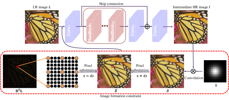
Figure 2: An overview of the proposed method. The image formation constraint is enclosed in the dotted red box, which is used to constrain a deep CNN for super-resolution. At each stage, our algorithm first generates an intermediate HR image ${I}$ by a deep CNN model and updates the intermediate HR image ${I}$ according to the image formation of SR by the pixel substitution (5). The updated image $\hat{B}$ is then taken as an input for the next stage. The network is solved in a cascaded manner and generates better high-quality images.

3 Image Formation Process

We first describe the image formation process of the SR problem and then derive the image formation constraint. Given a HR image $I$, the process of generating the LR image $L$ is usually defined as

$$L=\downarrow^{s}(k\otimes I),$$ (1)

where $k$ denotes the blur kernel, $\otimes$ denotes the convolution operator, and $\downarrow^{s}$ denotes the downsampling operation with a scale factor $s$. Mathematically, this image formation process can be rewritten as

$$\mathbf{L}=\mathbf{DK}\mathbf{I},$$ (2)

where $\mathbf{K}$ denotes the filtering matrix corresponding to the blur kernel $k$; $\mathbf{D}$ denotes the downsampling operation; $\mathbf{L}$ and $\mathbf{I}$ denote the vector forms of $L$ and $I$.

Applying the upsampling matrix, i.e., $\mathbf{D}^{\top}$, we have

$$\mathbf{D}^{\top}\mathbf{L}=\mathbf{D}^{\top}\mathbf{DK}\mathbf{I},$$ (3)

where $\mathbf{D}^{\top}\mathbf{D}$ is a selection matrix which is defined as

$$\mathbf{D}^{\top}\mathbf{D}(\mathrm{x},\mathrm{y})=\left\{\begin{array}[]{ll}1,&\mbox{}\ \mathrm{x}=\mathrm{y}=ds,\\ 0,&\mbox{}\ $otherwise$,\end{array}\right.$$ (4)

where $\mathrm{x}$ and $\mathrm{y}$ denote pixel locations; $d=\{1,\ldots,P\}$, and $P$ denotes the number of the pixels in $L$. If $\mathbf{D}^{\top}\mathbf{D}(\mathrm{x},\mathrm{x})=1$, we denote $\mathrm{x}$ as the un-decimated position. The constraint (3) indicates that the pixel value of $\mathrm{x}$ in ${L}$ is equal to the pixel value of $s\mathrm{x}$ in the blurred high resolution image $\mathbf{B}=\mathbf{KI}$ at the un-decimated positions. In the following, we will use the image formation constraint (3) to guide our SR algorithm so that it can generate high-resolution images satisfying this constraint.

Table 1: Network parameters. ResBlock denotes the residual block (?) which is used in (?).

Layers	Conv1	ResBlock	Conv2	Conv3
Filter size	3	3	3	3
Filter numbers	256	256	256	3
Stride	1	1	1	1

4 Proposed Algorithm

The analysis above inspires us to use the image formation process to constrain the deep neural networks for SR. Specifically, we first generate an intermediate HR image $I$ from a LR image $L$ by a deep neural network. Then we apply the convolution kernel to $I$ and use pixel substitution (Section 4.2) to enforce the image formation constraint in the feedback step, as shown in Figure 2. In the following, we will explain the details of the proposed algorithm.

4.1 Intermediate HR image estimation

The effectiveness of using deep CNNs to super-resolve images has been extensively validated in SR problems. Our goal here is not to propose a novel network structure but to develop a new framework to constrain the generated SR results using the image formation process. Thus, we can use an existing network architecture, such as EDSR (?), SRCNN (?), and VDSR (?). In this paper, we use similar network architecture by (?) as our HR image estimation sub-network. Figure 2 shows the proposed network architecture for one stage of the proposed cascaded approach. The parameters of the network are shown in Table 1, where we use $32$ ResBlocks and $0.1$ as the residual scaling factor (?).

4.2 Pixel substitution

Let ${I}$ be the output of the HR image estimation sub-network. If ${I}$ is the ground truth HR image, the equality in the SR formation model (3) strictly holds. Thus, to enforce the intermediate HR image ${I}$ to be close to the ground truth HR image, we adopt the pixel substitution operation (?). Specifically, we first obtain the upsampled image $\mathbf{D}^{\top}\mathbf{L}$ by applying the upsampling matrix $\mathbf{D}^{\top}$ to the LR image $\mathbf{L}$. Then we obtain the blurred intermediate HR image $\mathbf{B}$ and by applying the blur kernel $\mathbf{K}$ to the intermediate HR image $\mathbf{I}$. The output of the pixel substitution operation is

$$\mathbf{\hat{B}}(\mathrm{x})=\left\{\begin{array}[]{ll}\mathbf{D}^{\top}\mathbf{L}(\mathrm{x}),&\mbox{}\ \mathrm{x}=ds,\\ \mathbf{B}(\mathrm{x}),&\ $otherwise$.\end{array}\right.$$ (5)

Empirically, we find that the approximation scheme for image formation process converges well, as shown in the supplemental material.

Table 2: Quantitative evaluations of the state-of-the-art super-resolution methods on the benchmark datasets (Set5, Set14, B100, Urban100, Manga109, and DIV2K) in terms of PSNR and SSIM.

		Set5	Set14	B100	Urban100	Manga109	DIV2K (validation)
Algorithms	Scale	PSNR/SSIM	PSNR/SSIM	PSNR/SSIM	PSNR/SSIM	PSNR/SSIM	PSNR/SSIM
Bicubic	$\times 2$	33.66/0.9299	30.24/0.8688	29.56/0.8431	26.88/0.8403	30.80/0.9339	32.45/0.9040
A+	$\times 2$	36.54/0.9544	32.28/0.9056	31.21/0.8863	29.20/0.8938	35.37/0.9680	34.56/0.9330
SRCNN	$\times 2$	36.66/0.9542	32.45/0.9067	31.36/0.8879	29.50/0.8946	35.60/0.9663	34.59/0.9320
FSRCNN	$\times 2$	37.05/0.9560	32.66/0.9090	31.53/0.8920	29.88/0.9020	36.67/0.9710	34.74/0.9340
VDSR	$\times 2$	37.53/0.9590	33.05/0.9130	31.90/0.8960	30.77/0.9140	37.22/0.9750	35.43/0.9410
LapSRN	$\times 2$	37.52 0.9591	33.08/0.9130	31.08/0.8950	30.41/0.9101	37.27/0.9740	35.31/0.9442
MemNet	$\times 2$	37.78/0.9597	33.28/0.9142	32.08/0.8978	31.31/0.9195	37.72/0.9740	NA/NA
DRCN	$\times 2$	37.63/0.9588	33.04/0.9118	31.85/0.8942	30.75/0.9133	37.57/0.9730	35.45/0.940
EDSR	$\times 2$	38.19/0.9609	33.92/0.9195	32.35/0.9019	32.97/0.9358	39.20/0.9783	36.56/0.9485
RDN	$\times 2$	38.24/0.9614	34.01/0.9212	32.34/0.9017	32.89/0.9353	39.18/0.9780	36.52/0.9483
DBPN	$\times 2$	38.09/0.9600	33.85/0.9190	32.27/0.9000	32.55/0.9324	38.89/0.9775	36.37/0.9475
Ours	$\times 2$	38.26/0.9614	33.99/0.9200	32.37/0.9020	33.09/0.9365	39.26/0.9784	36.60/0.9487
Bicubic	$\times 3$	30.39/0.8682	27.55/0.7742	27.21/0.7385	24.46/0.7349	26.95/0.8556	29.66/0.8310
A+	$\times 3$	32.58/0.9088	29.13/0.8188	28.29/0.7835	26.03/0.7973	29.93/0.9120	31.09/0.8650
SRCNN	$\times 3$	32.75/0.9090	29.30/0.8215	28.41/0.7863	26.24/0.7989	30.48/0.9117	31.11/0.8640
FSRCNN	$\times 2$	33.18/0.9140	29.37/0.8240	28.53/0.7910	26.43/0.8080	31.10/0.9210	31.25/0.8680
VDSR	$\times 3$	33.67 0.9210	29.78 0.8320	28.83 0.7990	27.14 0.8290	32.01 0.9340	31.76/0.8780
LapSRN	$\times 3$	33.82/0.9227	29.87/0.8320	28.82/0.7980	27.07/0.8280	32.21/0.9350	31.22/0.8600
MemNet	$\times 3$	34.09/0.9248	30.00/0.8350	28.96/0.8001	27.56/0.8376	32.51/0.9369	NA/NA
DRCN	$\times 3$	33.82/0.9226	29.76/0.8311	28.80/0.7963	27.15/0.8276	30.97/0.8860	31.79/0.8770
EDSR	$\times 3$	34.68/0.9293	30.52/0.8462	29.26/0.8096	28.81/0.8658	34.19/0.9485	32.75/0.8933
RDN	$\times 3$	34.71/0.9296	30.57/0.8468	29.26/0.8093	28.80/0.8653	34.13/0.9484	32.73/0.8929
Ours	$\times 3$	34.75/0.9298	30.61/0.8466	29.29/0.8102	28.97/0.8683	34.14/0.9490	32.79/0.8939
Bicubic	$\times 4$	28.42/0.8104	26.00/0.7027	25.96 0.6675	23.14/0.6577	24.89/0.7866	28.11/0.7750
A+	$\times 4$	30.28/0.8603	27.32/0.7491	26.82/0.7087	24.32/0.7183	27.03/0.8510	29.28/0.8090
SRCNN	$\times 4$	30.48/0.8628	27.50/0.7513	26.90/0.7101	24.52/0.7221	27.58/0.8555	29.33/0.8090
FSRCNN	$\times 4$	30.72/0.8660	27.61/0.7550	26.98/0.7150	24.62/0.7280	27.90/0.8610	29.36/0.8110
VDSR	$\times 4$	31.35/0.8830	28.02/0.7680	27.29/0.0726	25.18/0.7540	28.83 0.8870	29.82/0.8240
LapSRN	$\times 4$	31.54/0.8850	28.19/0.7720	27.32/0.7270	25.21/0.7560	29.09/0.8900	29.88/0.8250
MemNe	$\times 4$	31.74/0.8893	28.26/0.7723	27.40/0.7281	25.50/0.7630	29.42/0.8942	NA/NA
DRCN	$\times 4$	31.53/0.8854	28.02/0.7670	27.23/0.7233	25.14/0.7510	28.97/0.8860	29.83/0.8230
EDSR	$\times 4$	32.48/0.8985	28.80 0.7876	27.72/0.7419	26.65/0.8032	31.03/0.9156	30.73/0.8445
RDN	$\times 4$	32.47/0.8990	28.81/0.7871	27.72/0.7419	26.61/0.8028	31.00/0.9151	30.71/0.8442
DBPN	$\times 4$	32.47/0.8980	28.82/0.7860	27.72/0.7400	26.38/0.7946	30.91/0.9137	30.66/0.8424
Ours	$\times 4$	32.56/0.8995	28.80/0.7882	27.73/0.7422	26.72/0.8053	31.06/0.9169	30.74/0.8450

4.3 Cascaded training

As the proposed algorithm consists of both intermediate HR image estimation and pixel substitution, we perform these two steps in a cascaded manner. Let $\Theta_{t}$ denote the model parameters at stage (iteration) $t$, and $\{L^{n},I_{gt}^{n}\}_{n=1}^{N}$ denote a set of $N$ training samples. We learn the stage-dependent model parameters $\Theta_{t}$ from $\{L^{n},I_{gt}^{n}\}_{n=1}^{N}$ by minimizing the cost function

$$\mathcal{J}(\Theta_{t})=\sum_{n=1}^{N}\|{I}_{t}^{n}-I_{gt}^{n}\|_{1},$$ (6)

where $I_{t}^{n}$ is the output of the network at the $t$-th stage. Following (?), we use $L_{1}$ norm as the loss function. We minimize (6) to learn the model parameters $\Theta_{t}$ stage by stage from $t=1,...,T$.

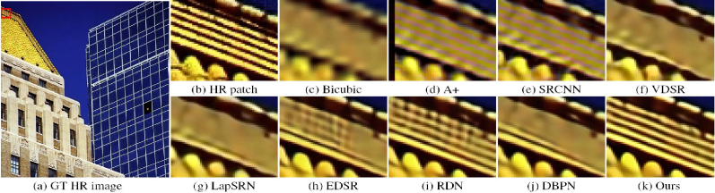
Figure 3: Visual comparisons for $4\times$ SR from the Urban100 dataset. The proposed algorithm generates much better results with fine detailed structures.

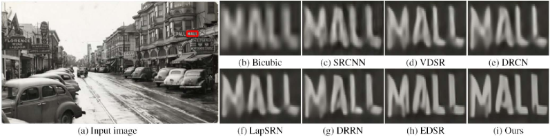
Figure 4: Results on real example ($\times 4$). The proposed method recovers much clearer images with better detailed structures.

5 Experimental Results

We examine the proposed algorithm using publicly available benchmark datasets and compare it to state-of-the-art single image SR methods. Due to the extensive experiments performed, we only show a small portion of the results in the main paper. Please see the supplementary document for more results.

5.1 Parameter settings and training data

In the learning process, we use the ADAM optimizer (?) with parameters $\beta_{1}=0.9$, $\beta_{2}=0.999$, and $\epsilon=10^{-8}$. The minibatch size is set to be $1$. The learning rate is initialized to be $10^{-4}$. We use a Gaussian kernel in (3) with the same settings used in (?). We empirically set $T=3$ as a trade-off between accuracy and speed. In the first stage, we use the same upsampling layer as (?) to upsample the features before the Conv₃ layer.

For fair comparisons, we first follow standard protocols adopted by existing methods (e.g., (?; ?; ?; ?)) to generate LR images using bicubic downsampling from the DIV2K dataset (?) for training and use the Set5 (?) as the validation test set. Then, we evaluate the effectiveness of our algorithm when LR images are obtained with different image formation models of SR in Section 6. We implement our algorithm based on the PyTorch version of (?). The code and trained models are publicly available on the authors websites.

5.2 Comparisons with the state of the art

To evaluate the performance of the proposed algorithm, we compare it against state-of-the-art algorithms including A+ (?), SRCNN (?), FSRCNN (?), VDSR (?), LapSRN (?), MemNet (?), DRCN (?), DRRN (?), EDSR (?), RDN (?), and DBPN (?). We use the benchmark datasets: Set5 (?), Set14 (?), B100 (?), Urban100 (?), Manga109 (?), and DIV2K (validation set) (?) to evaluate the performance. These datasets contain different image diversities, e.g., the Set5, Set14, and B100 datasets consist of natural scenes; Urban100 mainly contains urban scenes with details in different frequency bands; Manga109 is a dataset of Japanese manga; DIV2K (validation set) contains 100 natural images with 2K resolution. We use the PSNR and SSIM to evaluate the quality of each recovered image.

Table 2 summarizes the quantitative results on these benchmark datasets for the upsampling factors of 2, 3, and 4. Overall, the proposed method performs favorably against the state-of-the-art methods.

Figure 3 shows SR results with a scale factor of 4 by the evaluated methods. The results by the feed-forward models (?; ?; ?; ?; ?; ?) do not recover the structures well. The DBPN algorithm (?) adopts a feedback network to super-resolve images using information from the LR images. However, this method needs to regenerate LR featrues from intermediate HR features. Consequently, the information at un-decimated pixels would get lost, which makes it hard to estimate the details and structures. The results in Figure 3(j) show that the structures of the images super-resolved by the DBPN method are not recovered well. In contrast, the proposed method recovers finer image details and structures than the state-of-the-art algorithms.

Real examples.

We further evaluate our algorithm using real images (Figure 4). Our algorithm generates much clearer images with better detailed structures than those by the state-of-the-art methods (?; ?; ?; ?). For example, all the four letters in our result are legible, especially “A” (Figure 4(i)).

6 Analysis and Discussions

We have shown that enforcing the image formation constraint using pixel substitution leads to an algorithm that outperforms state-of-the-art methods. To better understand the proposed algorithm, we perform further analysis, compare it with related methods, and discuss its limitations.

Figure 5: Effectiveness of the image formation constraint ($\times$4). The image formation plays an important role for the details and structures estimation.

Table 3: Effectiveness of the image formation constraint in SR with the scale factor 2. “w/ only one stage” means the baseline method (?). “Stage 1”, “Stage 2”, “Stage 3” denote the intermediate results from stages 1, 2, and 3 of the proposed method, respectively. Other notations are detailed in the main context.

Dataset	Set5	B100	Urban100	Manga109
	PSNR/SSIM	PSNR/SSIM	PSNR/SSIM	PSNR/SSIM
w/o conv. & (5)	38.20/0.9612	32.33/0.9017	32.78/0.9347	39.07/0.9780
w/ only one stage	38.19/0.9609	32.35/0.9019	32.97/0.9358	39.20/0.9783
one stage with (7)	38.22/0.9613	32.33/0.9014	32.82/0.9351	39.00/0.9777
Stage 1	38.23/0.9613	32.34/0.9017	32.86/0.9350	39.15/0.9782
Stage 2	38.27/0.9614	32.36/0.9020	33.04/0.9362	39.26/0.9784
Stage 3	38.26/0.9614	32.37/0.9020	33.09/0.9365	39.26/0.9784

Effectiveness of the image formation constraint.

As our cascaded architecture uses a basic SR network several times, one may wonder whether the performance gains merely come from the use of a larger network. To answer this question, we remove the pixel substitution step from our cascaded network architecture (denoted as “w/o conv. & (5)”) for fair comparisons. The comparisons in Figure 5(d) and (f) demonstrate the benefit of using the image formation constraint in generating clearer images with finer details and structures. We note that there is little performance improvement by simply cascading a basic SR network several times to increase the network capacity (Figure 5(d)). The results in Table 3 show that using the image formation constraint of SR consistently improves SR results, which further demonstrates the effectiveness of this constraint.

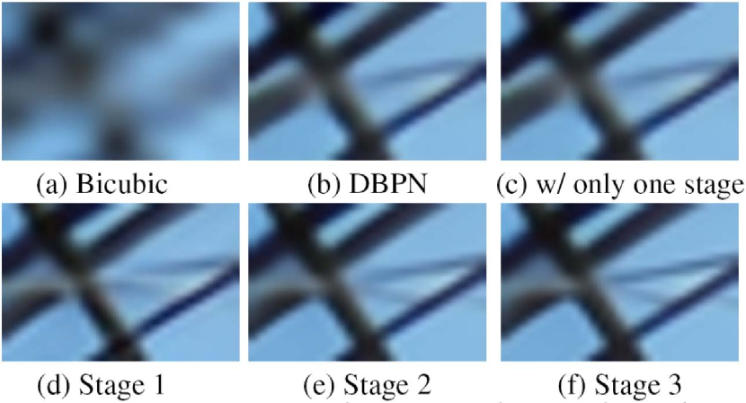
Figure 7: Effectiveness of the proposed stage-dependent algorithm ($\times$4). (c) denotes the results with only one stage. (d)-(f) denote the intermediate HR images from stage 1, 2, and 3, respectively.

Figure 7 shows some intermediate HR images from the proposed method. We note that the structural details are better recovered with more stages. This further demonstrates that using the image formation constraint in a deep CNN helps the restoration of the structural details.

As the proposed network architectures are similar to those used in (?), the proposed algorithm with only one stage would reduce to the feed-forward model (?) to some extent. Both the quantitative evaluations in Table 3 and comparisons in Figure 5(c) show that only using one feed-forward model does not generate high-quality HR images.

We further note that an alternative approach is to add the image formation model (1) to the loss function to constrain the network training instead of using feedback scheme, where the new loss function is defined as

$$\ell_{p}(I;I_{gt};L)=\|{I}-I_{gt}\|_{1}+\lambda\|\downarrow^{s}(k\otimes I)-L\|_{1},$$ (7)

where $\lambda$ is a weight parameter. We empirically set $\lambda=0.01$ for fair comparisons in this paper. We denote this baseline method as “one stage with (7)”. We quantitatively evaluate this baseline model on the benchmark datasets. Both the quantitative results in Table 3 and visual comparison (Figure 5(e)) demonstrate that adding the image formation loss to the overall loss function does not always improve the performance.

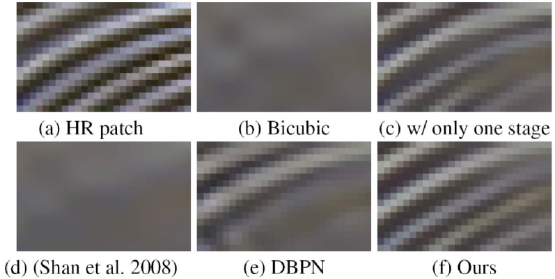
Figure 6: Comparisons of the results by different back-projection methods ($\times$4). The DBPN method based on the iterative back-projection algorithm (?) is less effective for the edges restoration due to the additional downsampling operation.

Closely-related methods.

Several notable methods (?; ?) improve the back-projection algorithm (?) for single image SR. The DBPN algorithm (?) extends the back-projection method (?) using a deep neural network. It needs a downsampling operation after obtaining intermediate HR images in the feedback stage. As the information at un-decimated pixels of the intermediate HR images may be lost due to the downsampling operation, DBPN is less effective at recovering details and structures (Figure 6(e)). The method (?) first proposes pixel substitution to enforce the image formation constraint in an iterative optimization scheme. However, this method cannot effectively restore the edges and textures (Figure 6(d)) because only the sparsity of gradient prior is used. In contrast, our algorithm uses pixel substitution to constrain the deep CNN. Both the edges and textures are well recovered (see Figure 6(f)).

We further examine whether the estimated HR images satisfy the image formation constraint. To this end, we apply the image formation to the estimated HR images to generate the LR images and use the PSNR and mean squared error (MSE) as the metrics. The MSE values in Table 4 indicate that the results generated by the proposed method satisfy the image formation model well.

Table 4: Evaluations of the regenerated LR images ($\times 2$).

Dataset	Set5	B100	Urban100	Manga109
	PSNR/MSE	PSNR/MSE	PSNR/MSE	PSNR/MSE
DBPN	61.60/0.0462	60.07/0.0704	59.00/0.0944	60.41/0.0658
Ours	72.06/0.0045	66.29/0.0264	65.04/0.0360	67.56/0.0189

Robustness to general degradation models of SR.

We have shown that using the image formation constraint can make the deep CNNs more compact thus facilitating the SR problem when the degradation model is approximated by the Bicubic downsmapling operation in Section 5.1. We further evaluate the proposed algorithm when the degradation model is approximated by the Bicubic downsmapling with noise. To generate LR images for training, we add Gaussian noise to each LR image used in Section 5.1, where the noise level ranges from 0 to 10%. Table 5 shows that our algorithm is robust to image noise due to the cascaded optimization method. More results about other degradation models are included in the supplementary document.

All above results on both synthetic and real-world images demonstrate that the proposed algorithm can generalize well even though the image formation constraint is based on known blur kernels.

Table 5: Results ($\times 2$) on “Set5” with noisy input images.

Noise level	1%	2%	3%	4%
EDSR	38.19/0.9610	35.96/0.9387	35.03/0.9272	34.30/0.9179
RDN	38.16/0.9609	35.69/0.9382	35.02/0.9272	34.20/0.9176
Ours	38.21/0.9611	36.01/0.9389	35.06/0.9275	34.34/0.9184

Running time performance.

As our algorithm uses a cascaded architecture, it increases the computation. We examine the running time of the proposed algorithm and compare it with state-of-the-art methods on the Set5 dataset, as shown in Table 6. The proposed algorithm takes slightly more running time compared with the feed-forward models, e.g., (?; ?). The proposed algorithm is about $3$ times faster than the feedback DBPN method (?).

Limitations.

As our algorithm uses the known image formation of SR to approximate the unknown degradation model of SR, it is less effective when this approximation does not hold. Figure 8 shows an example with significant JPEG compression artifacts, where the image formation model of SR does not approximate the degradation caused by the image compression well. Our algorithm exacerbates the compression artifacts, while the results by the feed-forward models have few artifacts. Building the compression process into the network architecture is likely to reduce these artifacts.

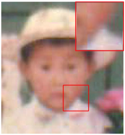
(a) Input image	(b) VDSR	(c) Ours

Figure 8: The proposed algorithm is less effective when the image formation of SR does not hold. Using the image formation of SR to super-resolve images with JPEG compression artifacts would exaggerate the artifacts (Best viewed on high-resolution display with zoom-in).

Table 6: Running time performance on SR with a scale factor of $2$.

Methods	VDSR	EDSR	RDN	DBPN	Ours
Avg. running time (/s)	0.88	1.16	2.01	6.81	2.21

7 Concluding Remarks

We have introduced a simple and effective super-resolution algorithm that exploits the image formation constraint. The proposed algorithm first uses a deep CNN to estimate an intermediate HR image and then uses pixel substitution to enforce the intermediate HR image satisfy the image formation model at the un-decimated pixel positions. Our cascaded architecture can be applied to existing feed-forward super-resolution networks. Both quantitative and qualitative results show that the proposed algorithm performs favorably against state-of-the-art methods.

Acknowledgement.

This work has been supported in part by the National Natural Science Foundation of China (Nos. 61922043, 61872421, 61732007) and the Natural Science Foundation of Jiangsu Province (No. BK20180471).

References

- [Bevilacqua et al. 2012] Bevilacqua, M.; Roumy, A.; Guillemot, C.; and Alberi-Morel, M. 2012. Low-complexity single-image super-resolution based on nonnegative neighbor embedding. In BMVC, 1–10.
- [Bulat, Yang, and Tzimiropoulos 2018] Bulat, A.; Yang, J.; and Tzimiropoulos, G. 2018. To learn image super-resolution, use a GAN to learn how to do image degradation first. In ECCV, 187–202.
- [Dong et al. 2014] Dong, C.; Loy, C. C.; He, K.; and Tang, X. 2014. Learning a deep convolutional network for image super-resolution. In ECCV, 184–199.
- [Dong, Loy, and Tang 2016] Dong, C.; Loy, C. C.; and Tang, X. 2016. Accelerating the super-resolution convolutional neural network. In ECCV, 391–407.
- [Han et al. 2018] Han, W.; Chang, S.; Liu, D.; Yu, M.; Witbrock, M.; and Huang, T. S. 2018. Image super-resolution via dual-state recurrent networks. In CVPR, 1654–1663.
- [Haris, Shakhnarovich, and Ukita 2018] Haris, M.; Shakhnarovich, G.; and Ukita, N. 2018. Deep back-projection networks for super-resolution. In CVPR, 1664–1673.
- [He et al. 2016] He, K.; Zhang, X.; Ren, S.; and Sun, J. 2016. Deep residual learning for image recognition. In CVPR, 770–778.
- [Huang, Singh, and Ahuja 2015] Huang, J.-B.; Singh, A.; and Ahuja, N. 2015. Single image super-resolution from transformed self-exemplars. In CVPR, 5197–5206.
- [Irani and Peleg 1991] Irani, M., and Peleg, S. 1991. Improving resolution by image registration. CVGIP: Graphical Model and Image Processing 53(3):231–239.
- [Kim, Lee, and Lee 2016a] Kim, J.; Lee, J. K.; and Lee, K. M. 2016a. Accurate image super-resolution using very deep convolutional networks. In CVPR, 1646–1654.
- [Kim, Lee, and Lee 2016b] Kim, J.; Lee, J. K.; and Lee, K. M. 2016b. Deeply-recursive convolutional network for image super-resolution. In CVPR, 1637–1645.
- [Kingma and Ba 2014] Kingma, D. P., and Ba, J. 2014. Adam: A method for stochastic optimization. CoRR abs/1412.6980.
- [Lai et al. 2017] Lai, W.-S.; Huang, J.-B.; Ahuja, N.; and Yang, M.-H. 2017. Deep laplacian pyramid networks for fast and accurate super-resolution. In CVPR, 624–632.
- [Ledig et al. 2017] Ledig, C.; Theis, L.; Huszar, F.; Caballero, J.; Cunningham, A.; Acosta, A.; Aitken, A. P.; Tejani, A.; Totz, J.; Wang, Z.; and Shi, W. 2017. Photo-realistic single image super-resolution using a generative adversarial network. In CVPR, 105–114.
- [Lim et al. 2017] Lim, B.; Son, S.; Kim, H.; Nah, S.; and Lee, K. M. 2017. Enhanced deep residual networks for single image super-resolution. In CVPR, 1132–1140.
- [Martin et al. 2001] Martin, D. R.; Fowlkes, C. C.; Tal, D.; and Malik, J. 2001. A database of human segmented natural images and its application to evaluating segmentation algorithms and measuring ecological statistics. In ICCV, 416–425.
- [Matsui et al. 2017] Matsui, Y.; Ito, K.; Aramaki, Y.; Fujimoto, A.; Ogawa, T.; Yamasaki, T.; and Aizawa, K. 2017. Sketch-based manga retrieval using manga109 dataset. Multimedia Tools Appl. 76(20):21811–21838.
- [Pan et al. 2018] Pan, J.; Liu, Y.; Dong, J.; Zhang, J.; Ren, J. S. J.; Tang, J.; Tai, Y.-W.; and Yang, M.-H. 2018. Physics-based generative adversarial models for image restoration and beyond. CoRR abs/1808.00605.
- [Sajjadi, Scholkopf, and Hirsch 2017] Sajjadi, M. S. M.; Scholkopf, B.; and Hirsch, M. 2017. Enhancenet: Single image super-resolution through automated texture synthesis. In ICCV, 4491–4500.
- [Shan et al. 2008] Shan, Q.; Li, Z.; Jia, J.; and Tang, C. 2008. Fast image/video upsampling. ACM TOG 27(5):153:1–153:7.
- [Shan, Jia, and Agarwala 2008] Shan, Q.; Jia, J.; and Agarwala, A. 2008. High-quality motion deblurring from a single image. ACM TOG 27(3):73:1–73:10.
- [Shi et al. 2016] Shi, W.; Caballero, J.; Huszar, F.; Totz, J.; Aitken, A. P.; Bishop, R.; Rueckert, D.; and Wang, Z. 2016. Real-time single image and video super-resolution using an efficient sub-pixel convolutional neural network. In CVPR, 1874–1883.
- [Tai et al. 2017] Tai, Y.; Yang, J.; Liu, X.; and Xu, C. 2017. Memnet: A persistent memory network for image restoration. In ICCV, 4539–4547.
- [Tai, Yang, and Liu 2017] Tai, Y.; Yang, J.; and Liu, X. 2017. Image super-resolution via deep recursive residual network. In CVPR, 3147–3155.
- [Timofte et al. 2017] Timofte, R.; Agustsson, E.; Gool, L. V.; Yang, M.; Zhang, L.; and et al. 2017. NTIRE 2017 challenge on single image super-resolution: Methods and results. In CVPR Workshops, 1110–1121.
- [Timofte, Smet, and Gool 2014] Timofte, R.; Smet, V. D.; and Gool, L. J. V. 2014. A+: adjusted anchored neighborhood regression for fast super-resolution. In ACCV, 111–126.
- [Tong et al. 2017] Tong, T.; Li, G.; Liu, X.; and Gao, Q. 2017. Image super-resolution using dense skip connections. In CVPR, 4799–4807.
- [Wang et al. 2015] Wang, Z.; Liu, D.; Yang, J.; Han, W.; and Huang, T. 2015. Deep networks for image super-resolution with sparse prior. In CVPR, 370–378.
- [Yang, Ma, and Yang 2014] Yang, C.-Y.; Ma, C.; and Yang, M. 2014. Single-image super-resolution: A benchmark. In ECCV, 372–386.
- [Zeyde, Elad, and Protter 2010] Zeyde, R.; Elad, M.; and Protter, M. 2010. On single image scale-up using sparse-representations. In The 7th International Conference on Curves and Surfaces, 711–730.
- [Zhang et al. 2017] Zhang, K.; Zuo, W.; Gu, S.; and Zhang, L. 2017. Learning deep CNN denoiser prior for image restoration. In CVPR, 2808–2817.
- [Zhang et al. 2018a] Zhang, Y.; Li, K.; Li, K.; Wang, L.; Zhong, B.; and Fu, Y. 2018a. Image super-resolution using very deep residual channel attention networks. In ECCV, 286–301.
- [Zhang et al. 2018b] Zhang, Y.; Li, K.; Li, K.; Wang, L.; Zhong, B.; and Fu, Y. 2018b. Image super-resolution using very deep residual channel attention networks. In ECCV, 294–310.
- [Zhang et al. 2018c] Zhang, Y.; Tian, Y.; Kong, Y.; Zhong, B.; and Fu, Y. 2018c. Residual dense network for image super-resolution. In CVPR, 2472–2481.