Coherence induced work in quantum heat engines with Larmor precession

Abstract

The impacts of quantum coherence on nonequilibrium thermodynamics become observable by dividing the heat and work into the conventional diagonal part and the other part relaying on the superpositions and the time derivative of Hamiltonian. Specializing to exactly-solvable dynamics of Larmor precession, we build a quantum Otto heat engine employing magnetic-driven atomic rotations. The coherence induced by the population transition guarantees the positive work output when the control protocol is time dependent. The time-dependent control of a quantum heat engine implements the correspondence between the classical and quantum adiabatic theorems for microscopic heat machines.

I INTRODUCTION

The first law of thermodynamics in any infinitesimal process can be expressed by taking the differential of the internal energy (key-1, ; key-2, ). For an open quantum system, the heat was defined originally by Alicki (key-3, 3, 4) as the non-unitary dissipative energy exchange due to the interaction between the system and the bath, while the work was described by the time-varying of Hamiltonian. Based on the first law of thermodynamics in the quantum domain, Kosloff et al. first did a systematic study of quantum heat engine (QHE) cycles working with harmonic oscillators and spins (key-5, 5, 6, 7, 8). Boukobza et al. extended Alicki’s formulas into the Heisenberg and interaction pictures and illustrated thermodynamics of bipartite systems (key-9, 9, 10). Quantum coherence may stimulate additional energy changes in thermodynamic processes, which has been observed by expressing the heat and work in term of the instantaneous orthonormal basis (key-11, 11, 12).

Nowadays, quantum thermodynamics has aroused general interest in both research and practice. Numerous unique properties arise due to quantum effects in the operation of microscopic heat engines. Klatzow et al. used nitrogen vacancy centers in the diamond to implement a three-level engine with long-lived coherence at the room temperature (key-13, ). Pekola et al. realised the miniature Otto cycle by exploiting the time-domain dynamics and coherence of driven superconducting qubits (key-14, 14, 15, 16). A quantum Otto heat engine (QOHE) operating under the reservoir at effective negative temperature was experimentally performed by employing Carbon-13 NMR spectroscopy (key-17, 17, 18). Quantum machines powered by nonthermal energy sources such as externally injected coherent atoms (key-19, 19, 20, 21) or squeezed baths (key-22, 22, 23, 24) have been shown to exhibit unconventional performances. Quantum optomechanical realization of a heat engine generates alternative strategies to extract work from the thermal energy of a mechanical resonator (key-25, 25, 26, 27). Other proposals may focus on QHEs when the fluctuation relation enters the conventional trade-off between the power and the efficiency (key-28, 28, 29, 30, 31).

However, a QOHE undergoes a four-step cycle where the two adiabatic branches involve the quantum adiabatic approximation. It means that a physical system should carry out a slow down evolution with a time-independent Hamiltonian ($\frac{\partial H}{\partial t}\rightarrow 0$) and remain in the instantaneous eigenstate corresponding to the initial Hamiltonian (key-32, 32, 33, 34). QOHEs based on quantum adiabatic processes are insufficient to incorporate quantum effects into the performance evaluation of a heat engine. Given this context, we are naturally led to consider the thermodynamic cycle applying time-varying Hamiltonians in the adiabatic processes. The thermodynamic quantities expressed in terms of the instantaneous eigenvectors of Hamiltonian allow estimating the capabilities of engines energised by quantum coherence.

In this work, based on the definitions of heat and work with respect to generic time-dependent open systems, a four-stroke power cycle, followed by thermodynamic adiabatic compression and expansion, and isochoric heat input and output, is built. We consider an atom driven by a rotating magnetic field as the working substance and give the formula of the work done when the atom experiences adiabatic evolution from an equilibrium state. How the quantum coherence induced by the transitions between different eigenstates influences the performance of a heat engine is waiting to be discovered. Importantly, we are interested in the correspondence between the classical and quantum adiabatic regimes for QHEs.

II HEAT AND WORK IN QUANTUM THERMODYNAMIC PROCESSES

To build a quantum heat engine, a preliminary and necessary step is to identify the heat and work in quantum regimes. In our previous study (key-11, 11), heat and work are classified on the basis of the time-dependent processes. According to the microscopic description of the first law of thermodynamics, the rates of the heat $\dot{Q}$ absorbed from the surroundings and the work $\dot{W}$ performed by the external field have the following forms

$$\dot{Q}=\sum_{n}\dot{\rho}_{nn}E_{n}-\sum_{n\neq m}\rho_{nm}\left\langle m\right|\frac{\partial\hat{H}}{\partial t}\left|n\right\rangle$$ (1)

and

$$\dot{W}=\sum_{n}\rho_{nn}\dot{E}_{n}+\sum_{n\neq m}\rho_{nm}\left\langle m\right|\frac{\partial\hat{H}}{\partial t}\left|n\right\rangle,$$ (2)

where $\left|m\left(t\right)\right\rangle$ denotes the instantaneous eigenstate of the Hamiltonian $\hat{H}(t)$ with the energy level $E_{m}\left(t\right)$, $\rho_{nm}\left(t\right)=\left\langle n\left(t\right)\right|\hat{\rho}\left|m\left(t\right)\right\rangle$ represents the element of the density matrix, and the dot indicates the time derivative. For simplicity purposes, the letter “(t)” is omitted in Eqs. (1) and (2). It is worthy of note that Eq. (2) was also obtained in Ref. (key-12, 12).

When the quantum system is coupled to a heat bath and the Hamiltonian is time independent, i.e., $\frac{\partial\hat{H}}{\partial t}=0$ and $\dot{E}_{n}=0$, there is no work done by the external force $\left(\dot{W}=0\right)$. This process is considered to be isochoric exemplified by the heating or cooling of the working substance with $\dot{Q}=\sum_{n}\dot{\rho}_{nn}E_{n}$.

An adiabatic process occurs without the transfer of heat or mass between the system and the environment. Therefore, the alteration of the internal energy exists in the form of work only. The Liouville-von Neumann equation describes how the density operator evolves in time (key-35, 35), i.e.,

$$\dot{\hat{\rho}}=-\frac{i}{\hbar}\left[\hat{H},\hat{\rho}\right].$$ (3)

Replacing the operator in a matrix form, we are capable of reaching the equality

$$\sum_{n}\dot{\rho}_{nn}E_{n}=\sum_{n\neq m}\rho_{nm}\left\langle m\right|\frac{\partial\hat{H}}{\partial t}\left|n\right\rangle,$$ (4)

which indicates that $\dot{Q}=0$. The quantum coherence, represented by $\sum_{n\neq m}\rho_{nm}\left\langle m\right|\frac{\partial\hat{H}}{\partial t}\left|n\right\rangle$, eliminates the heat loss to the surroundings in the thermodynamic adiabatic process.

Equations (1) and (2) give the general formulas of the heat and work in quantum thermodynamic processes, and are compatible with Alicki and Kieu’s definitions (key-3, 3, 36). The first term in Eq. (1) states that the change of the probabilities $\rho_{nn}$ generates the heat transfer. Work can be done by a system during a process that alters the energy levels $E_{n}$, as indicated by the first quantity of Eq. (2). The second parts in Eqs. (1) and (2) imply that $\dot{Q}$ and $\dot{W}$ are closely related to the quantum coherence if the Hamiltonian depends sensitively on time. In view of the expressions Eqs. (1) and (2), we are going to build a Otto quantum heat engine relying on a time-dependent adiabatic process [Fig. 1(a)].

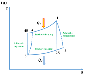
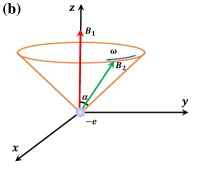
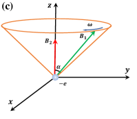
Figure 1: (a) The temperature–entropy (T–S) diagram of the quantum Otto heat engine based on the atomic Larmor precession. The process from 1 to 2 (3 to 4) represents the irreversible adiabatic compression (expansion) process, where the magnetic field [green arrows in (b) and (c)] starts to ride around at the intensity $B_{2}\left(B_{1}\right)$, angular velocity $\omega$, and incline angle $\alpha$. The process from 4 to 1 (2 to 3) denotes the isochoric heating (cooling) process, in which the system interacting with a time-independent magnetic field $\boldsymbol{B}=B_{1}\boldsymbol{e}_{z}\left(B_{2}\boldsymbol{e}_{z}\right)$ [red arrows in (b) and (c)] is put in thermal contact with a hot (cold) bath at the inverse temperature $\beta_{h}$ $\left(\beta_{c}\right)$. The evolutions from 1 to 2S and from 3 to 4S represent the quantum adiabatic processes with $\alpha=0$.

III THE ADIABATIC EVOLUTION OF THE ATOMIC SYSTEM FROM A STATE OF THERMAL EQUILIBRIUM

Before building a four-stroke cycle, one needs to understand the adiabatic dynamics of the working substance starting from the equilibrium state. The atomic Larmor precession allows us to extract work by considering an atom located at the origin of three-dimensional space and driven by a rotating magnetic field $\boldsymbol{B}\left(j,\alpha,t\right)=B_{j}[\sin\alpha\cos\left(\omega t\right)\boldsymbol{e}_{x}+\sin\alpha\sin\left(\omega t\right)\boldsymbol{e}_{y}+\cos\alpha\boldsymbol{e}_{z}]$ [$j=1$ and $2$, as shown in Figs. 1(b) and 1(c)]. Its Hamiltonian takes the form (key-37, 37)

$$\hat{H}\left(\omega_{j},\alpha,t\right) =-\hat{\mathbf{\mathbf{\boldsymbol{\mu}}}}\cdot\boldsymbol{B}\left(j,\alpha,t\right)=\frac{\hbar\omega_{j}}{2}$$

$$\times[\sin\alpha\cos\left(\omega t\right)\hat{\sigma}_{x}+\sin\alpha\sin\left(\omega t\right)\hat{\sigma}_{y}+\cos\alpha\hat{\sigma}_{z}],$$ (5)

where the atom has the mass $m$ and charge $-e$; $\mathbf{\hat{\mathbf{\mathbf{\boldsymbol{\mu}}}}}=\gamma_{e}\hat{\boldsymbol{S}}$ is the dipole moment determined by the gyromagnetic ratio $\gamma_{e}=-e/m$ and spin angular momentum $\hat{\boldsymbol{S}}$; $\hat{\sigma}_{i}$ ($i=x$, $y$, and $z$) define the Pauli spin matrices; $\omega_{j}=eB_{j}/m$; and $\hbar$ equals the Planck constant divided by $2\pi$.

From the orthonormal basis $\left|\uparrow\right\rangle=\left(\begin{array}[]{c}1\\ 0\end{array}\right)$ and $\left|\downarrow\right\rangle=\left(\begin{array}[]{c}0\\ 1\end{array}\right)$ , we can write out the normalized eigenstates of $\hat{H}\left(\omega_{j},\alpha,t\right)$ as

$$\left|\chi_{+}\left(\alpha,t\right)\right\rangle=\cos\frac{\alpha}{2}\left|\uparrow\right\rangle+e^{i\omega t}\sin\frac{\alpha}{2}\left|\downarrow\right\rangle$$ (6)

and

$$\left|\chi_{-}\left(\alpha,t\right)\right\rangle=e^{-i\omega t}\sin\frac{\alpha}{2}\left|\uparrow\right\rangle-\cos\frac{\alpha}{2}\left|\downarrow\right\rangle,$$ (7)

which represent the spin up and down, respectively, along the instantaneous direction of $\boldsymbol{B}\left(t\right)$. The corresponding eigenvalues are

$$E_{\pm}\left(\omega_{j}\right)=\pm\frac{\hbar\omega_{j}}{2},$$ (8)

remaining unvarying over time.

By invoking the transformation $\hat{R}_{z}\left(t\right)=e^{i\omega t\hat{\sigma}_{z}/2}$, Eq. (8) reduces to

$$\hat{H}_{R} \left(\omega_{j},\alpha\right)=\hat{R}_{z}\left(t\right)\hat{H}\left(\omega_{j},\alpha,t\right)\hat{R^{\dagger}}_{z}\left(t\right)-i\hbar\hat{R}_{z}\left(t\right)\frac{\partial}{\partial t}\hat{R^{\dagger}}_{z}\left(t\right)$$

$$=\frac{\hbar}{2}\left[\omega_{j}\sin\alpha\hat{\sigma}_{x}+\left(\omega_{j}\cos\alpha-\omega\right)\hat{\sigma}_{z}\right].$$ (9)

In the rotating frame, the effective Hamiltonian $\hat{H}_{R}\left(\omega_{j},\alpha\right)$ contains no explicit time dependence, yielding the evolution operator

$$\hat{U_{R}}\left(\omega_{j},\alpha,t\right) =e^{-i\hat{H}_{R}\left(\omega_{j},\alpha\right)t/\hbar}$$

$$=\cos\varOmega_{j}t/2-i\frac{\omega_{j}\sin\alpha\sin\varOmega_{j}t/2}{\varOmega_{j}}\hat{\sigma}_{x}$$

$$-i\frac{\left(\omega_{j}\cos\alpha-\omega\right)\sin\varOmega_{j}t/2}{\varOmega_{j}}\hat{\sigma}_{z}.$$ (10)

In Eq. (10), $\varOmega_{j}=\sqrt{\left(\omega_{j}\cos\alpha-\omega\right)^{2}+\omega_{j}^{2}\sin^{2}\alpha}$, and the relation $e^{i\mathbf{\hat{\sigma}}\cdot\mathbf{A}}=\cos A+i\frac{\mathbf{\hat{\sigma}}\cdot\mathbf{A}}{A}\sin A$ [$\mathbf{\hat{\sigma}}=\hat{\sigma}_{x}+\hat{\sigma}_{y}+\hat{\sigma}_{z}$, and $A=\left|\mathbf{A}\right|$ ] has been applied. The evolution operator in the original frame reads

$$\hat{U}\left(\omega_{j},\alpha,t\right) =\hat{R^{\dagger}}_{z}\left(t\right)\hat{U_{R}}\left(\omega_{j},\alpha,t\right)=\left(\begin{array}[]{cc}e^{-i\omega t/2}&0\\ 0&e^{i\omega t/2}\end{array}\right)$$ (13)

$$\times\left(\begin{array}[]{c}\cos\varOmega_{j}t/2-i\frac{\omega_{j}\cos\alpha-\omega}{\varOmega_{j}}\sin\varOmega_{j}t/2\\ -i\frac{\omega_{j}\sin\alpha}{\varOmega_{j}}\sin\varOmega_{j}t/2\end{array}\right.$$ (16)

$$\left.\begin{array}[]{c}-i\frac{\omega_{j}\sin\alpha}{\varOmega_{j}}\sin\varOmega_{j}t/2\\ \cos\varOmega_{j}t/2+i\frac{\omega_{j}\cos\alpha-\omega}{\varOmega_{j}}\sin\varOmega_{j}t/2\end{array}\right).$$ (19)

The unitary operator immediately allows us to understand the dynamic behaviors of the atom.

As an illustrative example, we consider the system initially in a state of thermal equilibrium (characterized by the ambient temperature $T$) subjected to a uniform magnetic field in the z-direction $\boldsymbol{B}\left(1,0,0\right)=B_{1}\boldsymbol{e}_{z}$ [red arrow in Fig. 1(b)]. Because $\hat{H}\left(\omega_{1},0,0\right)$ and $\hat{\sigma}_{z}$ commute, this canonical ensemble creates a diagonal density matrix in the $\hat{\sigma}_{z}$ basis, i.e.,

$$\hat{\rho}_{th}\left(\omega_{1},\beta\right)=\frac{\left(\begin{array}[]{cc}e^{-\beta\hbar\omega_{1}/2}&0\\ 0&e^{\beta\hbar\omega_{1}/2}\end{array}\right)}{Z\left(\omega_{1},\beta\right)}.$$ (20)

The partition function $Z\left(\omega_{1},\beta\right)=e^{-\beta\hbar\omega_{1}/2}+e^{\beta\hbar\omega_{1}/2}$. The inverse temperature $\beta=1/\left(k_{B}T\right)$, where $T$ is the effective temperature and $k_{B}$ is the Boltzmann constant.

For $t>0$, the magnetic field [green arrow in Fig. 1 (b)] makes a rotation around the z-axis, given by the vector $\boldsymbol{B}\left(2,\alpha,t\right)$. The time evolution of the density operator is obtained by the unitary transformation

$$\hat{\rho}\left(\omega_{2},\omega_{1},\alpha,\beta,t\right)=\hat{S}\left(\alpha,t\right)\hat{\rho}^{\ast}\left(\omega_{2},\omega_{1},\alpha,\beta,t\right)\hat{S}^{\dagger}\left(\alpha,t\right)$$ (21)

By defining the transformation matrix $\hat{S}\left(\alpha,t\right)=\left(\begin{array}[]{cc}\cos\frac{\alpha}{2}&e^{-i\omega t}\sin\frac{\alpha}{2}\\ e^{i\omega t}\sin\frac{\alpha}{2}&-\cos\frac{\alpha}{2}\end{array}\right)$, the matrix elements of $\hat{\rho}^{\ast}\left(\omega_{2},\omega_{1},\alpha,\beta,t\right)=\hat{U}\left(\omega_{2},\alpha,t\right)\rho_{th}\left(\omega_{1},\beta\right)\hat{U}^{\dagger}\left(\omega_{2},\alpha,t\right)$ have been written in terms of the eigenstates of the instantaneous Hamiltonian, which are, respectively, given by $\rho_{nm}\left(\omega_{2},\omega_{1},\alpha,\beta,t\right)=\left\langle\chi_{n}\left(\alpha,t\right)\right|\hat{\rho}\left(\omega_{2},\omega_{1},\alpha,\beta,t\right)\left|\chi_{m}\left(\alpha,t\right)\right\rangle$ ($\left\{n,m\right\}=\left\{+,+\right\}$, $\left\{-,-\right\}$, $\left\{+,-\right\}$, or $\left\{-,+\right\}$).

Most existing literatures studied the quantum thermodynamics based on the time-independent Hamiltonian or the quantum adiabatic theorem. Thus, Eqs. (1) and (2) reduce to $\dot{Q}=\sum_{n}\dot{\rho}_{nn}E_{n}$ and $\dot{W}=\sum_{n}\rho_{nn}\dot{E}_{n}$, meaning that the heat exchange merely depends on the population alteration and the work corresponds to the change of the eigenenergy spectrum (key-38, 38, 39, 40). However, for the two-level system driven by a rotating magnetic field, the eigenvalues relating to the instantaneous eigenstates $\left|\chi_{+}\left(\alpha,t\right)\right\rangle$ and $\left|\chi_{-}\left(\alpha,t\right)\right\rangle$ are fixed values [Eq. (8)]. If the work flux in the thermodynamic adiabatic process remains being computed by $\dot{W}=\sum_{n}\rho_{nn}\left(\omega_{2},\omega_{1},\alpha,\beta,t\right)\dot{E}_{n}\left(\omega_{2}\right)$, one has $\dot{W}=0$. It is anormal that no work can be done by the rotating magnetic field $\boldsymbol{B}\left(2,\alpha,t\right)$. In addition, the time derivative of $\rho_{++}\left(\omega_{2},\omega_{1},\alpha,\beta,t\right)$ and $\rho_{--}\left(\omega_{2},\omega_{1},\alpha,\beta,t\right)$ arrives at $\dot{Q}=\dot{\rho}_{++}\left(\omega_{2},\omega_{1},\alpha,\beta,t\right)E_{+}\left(\omega_{2}\right)+\dot{\rho}_{--}\left(\omega_{2},\omega_{1},\alpha,\beta,t\right)E_{-}\left(\omega_{2}\right)=\frac{\hbar\omega\omega_{2}^{2}\sin\varOmega_{2}t\sin^{2}\alpha\tanh\left(\frac{\beta\hbar\omega_{1}}{2}\right)}{2\varOmega_{2}}$. As $\dot{Q}$ is a non-zero value, it appears unconvincing that the heat transfer between the system and the environment exists in the thermodynamic adiabatic process.

For these reasons, the second terms on the right of Eqs. (1) and (2) quantifying quantum coherence play an indispensable role in the formulation of the first law of thermodynamics. Making use of Eq. (5) and taking the off-diagonal elements of the density operator in Eq. (13), one readily gets

$$\sum_{n\neq m}\rho_{nm}\left(\omega_{2},\omega_{1},\alpha,\beta,t\right)\left\langle m\right|\frac{\partial\hat{H}\left(\omega_{2},\alpha,t\right)}{\partial t}\left|n\right\rangle$$

$$=\frac{\hbar\omega\omega_{2}^{2}\sin\varOmega_{2}t\sin^{2}\alpha\tanh\left(\frac{\beta\hbar\omega_{1}}{2}\right)}{2\varOmega_{2}},$$ (22)

which satisfies $\sum_{n}\dot{\rho}_{nn}\left(\omega_{2},\omega_{1},\alpha,\beta,t\right)E_{n}\left(\omega_{2}\right)=\sum_{n\neq m}\rho_{nm}\left(\omega_{2},\omega_{1},\alpha,\beta,t\right)\left\langle m\right|\frac{\partial\hat{H}\left(\omega_{2},\alpha,t\right)}{\partial t}\left|n\right\rangle$ and the nonexistence of the heat transfer, i.e., $\dot{Q}=0$. As a result, the atomic Larmor precession could be regarded as a thermodynamic adiabatic process. We use

$$W_{L}\left(\omega_{2},\omega_{1},\alpha,\beta,t\right) =\int_{0}^{t}\sum_{n\neq m}\rho_{nm}\left(\omega_{2},\omega_{1},\alpha,\beta,t^{\prime}\right)$$

$$\times\left\langle m\right|\frac{\partial\hat{H}\left(\omega_{2},\alpha,t^{\prime}\right)}{\partial t^{\prime}}\left|n\right\rangle dt^{\prime}$$

$$=\frac{\hbar\omega\omega_{2}^{2}\sin^{2}\varOmega_{2}t/2\sin^{2}\alpha\tanh\left(\frac{\beta\hbar\omega_{1}}{2}\right)}{\varOmega_{2}^{2}}$$ (23)

to describe the work performed on the system due to the Larmor precession. It can be regarded as a coherence work induced by the transition between the instantaneous eigenstates $\left|\chi_{\pm}\left(\alpha,t\right)\right\rangle$ of the Hamiltonian $\hat{H}\left(\omega_{2},\alpha,t\right)$. The work performed by the external field beginning with the initial equilibrium state is calculated as

$$W\left(\omega_{2},\omega_{1},\alpha,\beta,t\right)=W_{L}\left(\omega_{2},\omega_{1},\alpha,\beta,t\right)+W_{S}\left(\omega_{2},\omega_{1},\alpha,\beta,t\right),$$ (24)

where $W_{S}\left(\omega_{2},\omega_{1},\alpha,\beta,t\right)=Tr\left(\left[\hat{H}\left(\omega_{2},\alpha,0\right)-\hat{H}\left(\omega_{1},0,0\right)\right]\hat{\rho}_{th}\left(\omega_{1},\beta\right)\right)+Tr\left(\left[\hat{H}\left(\omega_{2},0,t\right)-\hat{H}\left(\omega_{2},\alpha,t\right)\right]\hat{\rho}^{\ast}\left(\omega_{2},\omega_{1},\alpha,\beta,t\right)\right)$ includes the work contributed by Hamiltonian’s sudden shifts from $\hat{H}\left(\omega_{1},0,0\right)$ to $\hat{H}\left(\omega_{2},\alpha,0\right)$ and from $\hat{H}\left(\omega_{2},\alpha,t\right)$ to $\hat{H}\left(\omega_{2},0,t\right)$.

IV QUANTUM OTTO CYCLE

The quantum Otto cycle is composed of the thermodynamic adiabatic compression, rejection of heat at a constant external field, thermodynamic adiabatic expansion, and heat addition at another constant external field, as illustrated in Fig. 1 (a). The respective scheme of the four distinct strokes is described below.

At stage I (1-2), the atom is initially in thermal equilibrium state $\hat{\rho}_{1}=\hat{\rho}_{th}\left(\omega_{1},\beta_{h}\right)$ characterized by temperature $T_{h}=1K$. From time $t=0$ to $t=\tau_{1}$, the atom becomes isolated from the hot bath and experiences a thermodynamic adiabatic compression. The magnetic field is switched from $\boldsymbol{B}\left(1,0,0\right)$ [red arrow in Fig. 1(b)] to $\boldsymbol{B}\left(2,\alpha,0\right)$ [green arrow in Fig. 1(b)] and free to rotate around the z axis. The working medium unitarily evolves to the mixed state given by $\hat{\rho}_{2}=\hat{\rho}\left(\omega_{2},\omega_{1},\alpha,\beta_{h},\tau_{1}\right)$ [see Eq. (13)]. After the rotation, the magnetic field flips back to the direction of the z axis and remains unvarying over time, denoted by $\boldsymbol{B}\left(2,0,\tau_{1}\right)$. The work performed by the magnetic field increases the internal energy of the atom, that is,

$$W_{1}=W\left(\omega_{2},\omega_{1},\alpha,\beta_{h},\tau_{1}\right).$$ (25)

At stage II (2-3), the atom having probability of each eigenstate uniquely determined by $\hat{\rho}_{2}$ comes into contact with the cold bath at temperature $T_{c}=0.1K$. During the process of reaching thermal equilibrium, the removal of heat allows the atomic system to relax toward equilibrium state followed by the density operator $\hat{\rho}_{3}=\hat{\rho}_{th}\left(\omega_{2},\beta_{c}\right)$. Eigenvalues of the working medium depend only on the amplitude of the external field, which are kept fixed at $E_{\pm}\left(\omega_{2}\right)$ . According to Eqs. (1) and (2), the atom exchanges energy with the cold bath in the form of heat transfer and no work is performed by the magnetic field. The amount of the heat transfer between the atom and the cold bath is represented by

$$Q_{c} =-\frac{\hbar}{2}\omega_{2}\tanh\left(\frac{1}{2}\beta_{c}\hbar\omega_{2}\right)$$

$$-Tr\left(\hat{H}\left(\omega_{2},0,\tau_{1}\right)\hat{\rho}^{\ast}\left(\omega_{2},\omega_{1},\alpha,\beta_{h},\tau_{1}\right)\right).$$ (26)

At stage III (3-4), a process of thermodynamic adiabatic expansion would be carried out by isolating the atom from the cold bath and making the magnetic field whirl around in the duration between $t=0$ to $t=\tau_{2}$. The vector of the magnetic field transforms from $\boldsymbol{B}\left(2,0,0\right)$ [red arrow in Fig. 1(c)] to $\boldsymbol{B}\left(1,\alpha,t\right)$ [green arrow in Fig. 1(c)]. The Larmor frequency returns back to $\omega_{1}$ again, allowing the density operator to unitarily evolve to $\hat{\rho}_{4}=\hat{\rho}\left(\omega_{1},\omega_{2},\alpha,\beta_{c},\tau_{2}\right)$. In a similar way, we move the magnetic field in z direction instantly at time $\tau_{2}$, followed by $\boldsymbol{B}\left(1,0,\tau_{2}\right)$. With Eq. (15), the work done by the atom follows as

$$W_{2}=W\left(\omega_{1},\omega_{2},\alpha,\beta_{c},\tau_{2}\right).$$ (27)

At stage IV (4-1), since the Hamiltonian and the eigenenergies $E_{\pm}\left(\omega_{1}\right)$ are independent of time, a quantum isochoric evolution takes place without any work perform. The atom develops into the original canonical state $\hat{\rho}_{1}$ via thermalization with the hot bath at temperature $T_{h}$, which makes the heat engine operate automatically in a cyclic manner. At the end of this stage, the heat absorbed by the atom is written as

$$Q_{h} =-\frac{\hbar}{2}\omega_{1}\tanh\left(\frac{1}{2}\beta_{h}\hbar\omega_{1}\right)$$

$$-Tr\left(\hat{H}\left(\omega_{1},0,\tau_{2}\right)\hat{\rho}^{\ast}\left(\omega_{1},\omega_{2},\alpha,\beta_{c},\tau_{2}\right)\right).$$ (28)

After completing one cycle, the total energy contained within the atom always returns to its initial value. The net work of the cycle turns out to be

$$W=W_{1}+W_{2}=W_{L}+W_{S}.$$ (29)

The second equality means that the work has been partitioned into two distinct parts according to the separation in Eq. (15), where $W_{L(S)}=W_{L(S)}\left(\omega_{2},\omega_{1},\alpha,\beta_{h},\tau_{1}\right)+W_{L(S)}\left(\omega_{1},\omega_{2},\alpha,\beta_{c},\tau_{2}\right).$ For purposes of extracting work from the quantum heat engine, it is necessary that $W<0$. Using Eqs. (17)-(21), we obtain the expression of the efficiency as

$$\eta=\frac{-W}{Q_{h}}=1+\frac{Q_{c}}{Q_{h}}.$$ (30)

V RESULTS AND DISCUSSION

To build the complete descriptions of a quantum system in thermodynamic processes, it is important to explain how to differentiate between the quantum and thermodynamic adiabatic processes. For a quantum adiabatic process, if a system starts from an eigenstate of the initial Hamiltonian and the gaps among the eigenvalues exist, it will remain in the corresponding instantaneous eigenstate of the final Hamiltonian when the perturbation acting on it remains sufficiently slow (key-41, 41, 42), i.e., $\tau=\left|\hbar\left\langle m\right|\frac{\partial\hat{H}}{\partial t}\left|n\right\rangle/\left(E_{n}-E_{m}\right)^{2}\right|\ll 1\left(n\neq m\right)$. However, the first law of thermodynamics requires that a thermodynamic adiabatic process occurs with the rate of heat transfer $\dot{Q}=0$, relating the changes in internal energy only to the work done. The thermodynamic adiabatic process does not require the quantum adiabatic approximation to be satisfied (key-11, 11, 43).

In the case of a zero rotation angle $\alpha=0$, the atom-field interaction Hamiltonian becomes independent of time followed by $\frac{\partial\hat{H}\left(\omega_{j},\alpha,t\right)}{\partial t}=0$ [Eq. (5)]. The density operators of the four terminal states of the cycle [Fig. 1(a)] fulfill the relations $\hat{\rho}_{2}=\hat{\rho}_{1}=\hat{\rho}_{th}\left(\omega_{1},\beta_{h}\right)$ and $\hat{\rho}_{4}=\hat{\rho}_{3}=\hat{\rho}_{th}\left(\omega_{2},\beta_{c}\right)$ regardless of the time scales. The occupation probability of each instantaneous state remains unchanged during the transition from state 1 (3) to 2 (4), quantifying the applicability of quantum adiabatic approximations. The heat absorbed from the hot bath and the net work of the cycle could be, respectively, simplified as $Q_{h}=\frac{\hbar}{2}\omega_{1}\left[\tanh\left(\frac{1}{2}\beta_{c}\hbar\omega_{2}\right)-\tanh\left(\frac{1}{2}\beta_{h}\hbar\omega_{1}\right)\right]$ and $W=\frac{\hbar}{2}\left(\omega_{1}-\omega_{2}\right)\left[\tanh\left(\frac{1}{2}\beta_{h}\hbar\omega_{1}\right)-\tanh\left(\frac{1}{2}\beta_{c}\hbar\omega_{2}\right)\right]$. For the heat engine operating at the quantum adiabatic limit, $\omega_{2}/\omega_{1}>\beta_{h}/\beta_{c}$ is certainly a necessary condition to create useful work from the thermal energy. Meanwhile, the efficiency $\eta_{O}=1-\omega_{2}/\omega_{1}<1-\beta_{h}/\beta_{c}$, which is automatically less than the Carnot efficiency. These results appear consistent with prior researches based on two-level systems (key-6, 6, 44).

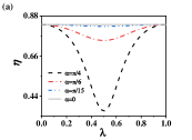
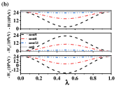
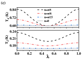
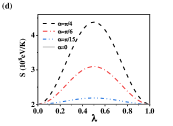
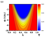
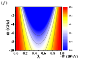
Figure 2: (a) The efficiency $\eta$, (b) work output $-W$, $-W_{L}$, and $-W_{S}$, (c) effective temperatures $T_{2}$ and $T_{4}$, and (d) entropy generation of the heat engine varying with the dimensionless time parameter $\lambda$ at $\omega=-6GHz$ and the inclination angles $\alpha=0$ (solid line, gray), $\pi/15$ (dash-double-dotted line, blue), $\pi/6$ (dash-dotted line, red), and $\pi/4$ (dash line, black). The contour plots of the (e) efficiency and (f) work output as functions of $\lambda$ and the angular velocity $\omega$ at $\alpha=\pi/4$. The parameters $T_{h}=1K$, $T_{c}=0.1K$, $\omega_{1}=6GHz$, and $\omega_{2}=1GHz$.

An investigation into the role of time-dependent protocol will focus on the numerical simulation. The efficiency $\eta$ and work output $-W$ exhibit periodicity with respect to the time spans of the thermodynamic adiabatic processes $\tau_{1}$ and $\tau_{2}$, which repeat over intervals of $2\pi/\varOmega_{1}$ and $2\pi/\varOmega_{2}$. By defining a dimensionless time parameter $\lambda=\frac{\tau_{1}\varOmega_{1}}{2\pi}=\frac{\tau_{2}\varOmega_{2}}{2\pi}$, Figs. 2 (a) and (b) show the curves of the efficiency $\eta$ and the work output $-W$ as functions of $\lambda$ at different values of $\alpha$. When the angle between the z axis and the vector of the field $\boldsymbol{B}\left(j,\alpha,t\right)$ goes to zero , i.e., $\alpha=0$, the efficiency reaches the Otto efficiency limit $\eta_{O}$ under a transitionless driving [solid line in Fig. 2(a)]. The efficiency converges to the same result at $\lambda=0$ or 1. This condition is equivalent to say that if the times for the adiabatic driving $\tau_{1}$ and $\tau_{2}$ become finite and are set to be integer multiples of $2\pi$, the heat engine will be operated in the quantum adiabatic regime as well. The work output $-W$ compromises the coherence work output $-W_{L}$ from the Larmor precession and the work output $-W_{S}$ due to the sudden change of field. $-W_{L}$ increases as $\alpha$ increases from $0$ to $\pi/4$, but $-W_{S}$ may turn negative [dash line in Fig. 2(b)]. Under these circumstances, the coherence work facilitates the normal operation of the quantum heat engine. From Figs. 2 (a) and (b), we conclude that the efficiency and net work output in the quantum adiabatic regime impose a theoretical limit of the heat engine with thermodynamic adiabatic processes. The changes of the probabilities of different eigenstates due to the non-ideal adiabatic processes ($\hat{\rho}_{2}\neq\hat{\rho}_{1}$ and $\hat{\rho}_{4}\neq\hat{\rho}_{3}$) occur in association with a supernumerary entropy production, increasing the irreversibility of the complete cycle.

By assuming that the ratio of the two occupation probabilities satisfies the Boltzmann distribution, the effective temperatures of the atom $T_{2}$ and $T_{4}$ at state 2 and 4 are, respectively, depending on the relations $\frac{\left\langle\chi_{+}\left(\alpha,\tau_{1}\right)\right|\hat{\rho}_{2}\left|\chi_{+}\left(\alpha,\tau_{1}\right)\right\rangle}{\left\langle\chi_{-}\left(\alpha,\tau_{1}\right)\right|\hat{\rho}_{2}\left|\chi_{-}\left(\alpha,\tau_{1}\right)\right\rangle}=e^{-\frac{E_{+}\left(\omega_{2}\right)-E_{-}\left(\omega_{2}\right)}{kT_{2}}}$ and $\frac{\left\langle\chi_{+}\left(\alpha,\tau_{2}\right)\right|\hat{\rho}_{4}\left|\chi_{+}\left(\alpha,\tau_{2}\right)\right\rangle}{\left\langle\chi_{-}\left(\alpha,\tau_{2}\right)\right|\hat{\rho}_{4}\left|\chi_{-}\left(\alpha,\tau_{2}\right)\right\rangle}=e^{-\frac{E_{+}\left(\omega_{1}\right)-E_{-}\left(\omega_{1}\right)}{kT_{4}}}$(key-17, 17). Figure 2 (c) demonstrates that the atom at state 2 is warmer than the cold bath ($T_{2}>T_{c}$) and give up its energy to the cold bath. Stage IV starts at a temperature smaller than that of the hot bath ($T_{4}<T_{h}$) . As a result, the heat engine is taking a quantity of heat energy from the hot bath until it reaches the equilibrium state. During a closed cycle, the atom returns to its original thermal state. The entropy generation per cycle $S=-\frac{Q_{h}}{T_{h}}-\frac{Q_{c}}{T_{c}}$. The entropy generation always remains positive without violating the second law of thermodynamics. Particularly, the quantum adiabatic regimes at $\alpha=0$ and $\lambda=0\left(1\right)$ allow a lower limit of $S$ to be obtained [Fig. 2(d)].

Under a time-dependent adiabatic evolution, the efficiency $\eta$ and work output $-W$ can be enhanced by modulating the dimensionless time parameter $\lambda$ and the angular velocity $\omega$ [Figs. 2 (e) and (f)]. For purposes of generating positive work to the environment regardless of the time spent in the adiabatic processes, the magnetic field should whirl around quickly. In the limit of $\omega\rightarrow\infty$ , $\underset{\omega\rightarrow\infty}{\lim}\hat{U}\left(\omega_{j},\alpha,t\right)=1$. As a result, the rapidly changing conditions prevent the system from adapting its configuration during the process, and the probabilities of the state remain unchanged. The efficiency is found close to the quantum adiabatic limit $\eta_{O}$ again. Based on the division of heat and work in thermodynamic processes with quantum coherence, one can conveniently design an efficient quantum Otto heat engine concerning the time-dependent control.

VI CONCLUSIONS

A simple model of the QOHE with a time-dependent adiabatic process is constructed in the frame of a spin driven by the rotating magnetic field. On the basis of the first law of thermodynamics premeditating the elements of quantum coherence, the work function relating to adiabatic evolution from an arbitrary equilibrium state is obtained. When the quantum cycle undergoes irreversible adiabatic processes, coherence induced population transition ensures that the heat engine can work properly. The efficiency and net work output at the quantum adiabatic speed limit set a upper bound for a QOHE under time-dependent control. The proposed model offers possible schemes to implement quantum cycles by manipulating a single nuclear spin via a sequence of suitable pulses and reconstructing the quantum state through the quantum state tomography.

References

• (1) R. Dann, A. Tobalina, and R. Kosloff, Phys. Rev. Lett. 122, 250402 (2019).
• (2) W. Niedenzu, V. Mukherjee, A. Ghosh, A. G. Kofman, and G. Kurizki, Nat. Commun. 9, 165 (2018).
• (3) R. Alicki, J. Phys. A: Math. Gen. 12, L103-L107 (1979).
• (4) F. Binder, L. A. Correa, C. Gogolin, J. Anders, G. Adesso, Thermodynamics in the Quantum Regime-Fundamental Aspects and New Directions, Switzerland, Springer, (2018).
• (5) R. Kosloff, J. Chem. Phys. 80, 1625-1631 (1984).
• (6) E. Geva and R. Kosloff, J. Chem. Phys. 96, 3054-3067 (1992).
• (7) Y. Rezek and R. Kosloff, New. J. Phys. 8, 83 (2006).
• (8) R. Kosloff, J. Chem. Phys. 150, 204105 (2019).
• (9) E. Boukobza and D. J. Tannor, Phys. Rev. Lett. 98, 240601 (2007).
• (10) E. Boukobza and D. J. Tannor, Phys. Rev. A 74, 063823 (2006).
• (11) S. Su, J. Chen, Y. Ma, J. Chen, and C. Sun, Chin. Phys. B 27, 060502 (2018).
• (12) K. Brandner, M. Bauer, and U. Seifert, Phys. Rev. Lett. 119, 170602 (2017).
• (13) J. Klatzow, J. N. Becker, P. M. Ledingham, C. Weinzetl, K. T. Kaczmarek, D. J. Saunders, J. Nunn, I. A. Walmsley, R. Uzdin, and E. Poem, Phys. Rev. Lett. 122, 110601 (2019).
• (14) A. Ronzani, B. Karimi, J. Senior, Y. Chang, J. T. Peltonen, C. Chen, and J. P. Pekola, Nat. Phys. 14, 991–995 (2018).
• (15) B. Karimi and J. P. Pekola, Phys. Rev. B 94, 184503 (2016).
• (16) J. P. Pekola, Nat. Phys. 11, 118–123 (2015).
• (17) R. J. de Assis, T. M. de Mendonça, C. J. Villas-Boas, A. M. de Souza, R. S. Sarthour, I. S. Oliveira, and N. G. de Almeida, Phys. Rev. Lett. 122, 240602 (2019).
• (18) T. B. Batalhão, A. M. Souza, L. Mazzola, R. Auccaise, R. S. Sarthour, I. S. Oliveira, J. Goold, G. De Chiara, M. Paternostro, and R. M. Serra, Phys. Rev. Lett. 113, 140601 (2014).
• (19) M. O. Scully, M. S. Zubairy, G. S. Agarwal, H. Walther, Science, 299, 862-864 (2003).
• (20) H. T. Quan, P. Zhang, and C. P. Sun, Phys. Rev. E 73, 036122 (2006).
• (21) M. T. Mitchison, M. P. Woods, J. Prior, and M. Huber, New J. Phys. 17, 115013 (2015).
• (22) J. Roßnagel, O. Abah, F. Schmidt-Kaler, K. Singer, and E. Lutz, Phys. Rev. Lett. 112, 030602 (2014).
• (23) J. Klaers, S. Faelt, A. Imamoglu, and E. Togan, Phys. Rev. X 7, 031044 (2017).
• (24) X. L. Huang, T. Wang, and X. X. Yi, Phys. Rev. E 86, 051105 (2012).
• (25) K. Zhang, F. Bariani, and P. Meystre, Phys. Rev. Lett. 112, 150602 (2014).
• (26) K. Zhang, F. Bariani, and P. Meystre, Phys. Rev. A 90, 023819 (2014).
• (27) A. Mari, A. Farace, and V. Giovannetti, J. Phys. B: At. Mol. Opt. Phys. 48, 175501 (2015).
• (28) G. Verley, M. Esposito, T. Willaert, and C. V. den Broeck, Nat. Commun. 5, 4721 (2014).
• (29) M. Campisi, J. Phys. A: Math. Theor. 47, 245001 (2014).
• (30) P. Pietzonka and U. Seifert, Phys. Rev. Lett. 120, 190602 (2018).
• (31) M. Bauer, K. Brandner, and U. Seifert, Phys. Rev. E 93, 042112 (2016).
• (32) H. Wang, J. He, and J. Wang, Phys. Rev. E 96, 012152 (2017).
• (33) Q. Liu, J. He, Y. Ma, and J. Wang, Phys. Rev. E 100, 012105 (2019).
• (34) C. Ou and S. Abe, Europhys. Lett. 113, 40009 (2016).
• (35) J. von Neumann, Mathematical foundations of quantum mechanics, Princeton, Princeton University Press (1955).
• (36) T. D. Kieu, Phys. Rev. Lett. 93, 140403 (2004).
• (37) D. J. Griffiths, Introduction to quantum mechanics, 2nd Ed., New Jersey, Prentice Hall (2005).
• (38) Y. Ma, S. Su, and C. Sun, Phys. Rev. E 96, 022143 (2017).
• (39) H. T. Quan, Phys. Rev. E 79, 041129 (2009).
• (40) G. A. Barrios, F. Albarrán-Arriagada, F. A. Cárdenas-López, G. Romero, and J. C. Retamal, Phys. Rev. A 96, 052119 (2017).
• (41) M. V. Berry, J. Phys. A: Math. Theor. 42, 365303 (2009).
• (42) C. P. Sun, J. Phys. A: Math. Gen. 21, 1595-1599 (1988).
• (43) H. T. Quan, Y. Liu, C. P. Sun, and F. Nori, Phys. Rev. E 76, 031105 (2007).
• (44) J. He, J. Chen, and B. Hua, Phys. Rev. E 65, 036145 (2002).