The Maximum Common Subgraph Problem: A Portfolio Approach

Abstract

The Maximum Common Subgraph is a computationally challenging problem with countless practical applications. Even if it has been long proven NP-hard, its importance still motivates searching for exact solutions. This work starts by discussing the possibility to extend an existing, very effective branch-and-bound procedure on parallel multi-core and many-core architectures. We analyze a parallel multi-core implementation that exploits a divide-and-conquer approach based on a thread-pool, which does not deteriorate the original algorithmic efficiency and it is not memory bound. We extend the algorithm to parallel many-core GPU architectures adopting the CUDA programming framework, and we show how to handle the heavily workload-unbalance and the massive data dependency. Then, we suggest new heuristics that reorder the adjacency matrix, deal with “dead-ends” and randomize the search with automatic restarts, achieving significant improvements on specific cases. Finally, we propose a portfolio approach, which integrates all the different local search algorithms as component tools. Such portfolio, rather than choosing the best tool for a given instance up-front, takes the decision on-line. The proposed approach drastically limits memory bandwidth constraints and avoids other typical portfolio fragilities as CPU and GPU versions often show a complementary efficiency and run on separated platforms. Experimental results support the claims and motivate further research to better exploit GPUs in embedded task-intensive, and multi-engine parallel applications.

=-15pt

I Introduction

Graphs are an extremely general and powerful data structure. They can be used to model, analyze and process a huge variety of phenomena and concepts by providing natural machine-readable representations. For instance, graphs may be used to represent the relationships between functions or fragments of code in programs, or the connections among functional blocks in electronic circuits.

The maximum common subgraph (MCS) problem consists in finding the largest graph which is simultaneously isomorphic to two subgraphs of two given graphs. The problem comes in two forms, namely the maximum common induced subgraph problem and the maximum common partial subgraph problem. In the former, the goal is to find a graph with as many vertices as possible which is an induced subgraph of each of two input graphs, that is, edges must be mapped to edges and non-edges, to non-edges. In the latter, conversely, the target is to find a common non-induced subgraph, with “partial” indicating that only all edges need to be mapped, while some edges might be skipped. In this paper, we discuss the induced variant, and for the sake of simplicity we will refer to it simply as the maximum common subgraph problem.

MCS problems arise in many areas, such as bioinformatics, computer vision, code analysis, compilers, model checking, pattern recognition, and have been discussed in literature since the seventies [1, 2]. MCS has been recognized as NP-hard problem, and it is computationally challenging in the general case: running state-of-the-art algorithms become computationally unfeasible on problems with as little as $40$ vertices, unless some meta information allows to reduce the search space. Practitioners from many fields are still asking researchers how to effectively tackle the problem in their real-world applications.

In 2017 McCreesh et al. [3] proposed McSplit, a very efficient branch-and-bound algorithm to find maximum common subgraphs for a large variety of graphs, such as, undirected, directed, labeled with several labeling strategies, etc. Essentially, McSplit is a recursive procedure adopting a smart invariant and an effective bound prediction formula. The invariant considers a new vertex pair, within the current mapping between the two graphs, only if the vertices within the pair share the same label, i.e., they are connected in the same way to all previously selected vertices. The bound consists in computing, from the current mapping size and from the labels of yet to map vertices, the maximum MCS size the current recursion path may lead to, and to prune those paths that are not promising enough.

In this paper, we extend McSplit in two directions. First, we present a multi-core and a many-core parallel implementations. In the former, CPU-based version, threads are organized in a thread pool, sharing a queue in which tasks are inserted by the the working thread and later extracted and solved by the first free helper thread. Mechanisms are used to avoid task duplication, task unbalance, and data structure repetition, as such problems may impair the original divide-and-conquer approach. Then, we analyze how to extend the approach to a many-core GPU, adopting the CUDA programming framework. We describe the corrections required to handle the heavy workload unbalance and the massive data dependency of the original, recursive algorithm.

After that, we extend the classical “winner-takes-all” approach to the MCS problem to a multi-engine methodology [4, 5, 6]. However, the structural properties of graphs not always relate with the difficulties faced by the MCS, and defining a representative set of problem instances to assess tools’ performances is not feasible. Unlikely standard multi-engine approaches, in the proposed solution the different algorithms run in parallel, and the algorithm selection is made on-line.

We insert in our portfolio the original sequential and parallel versions, improved with new heuristics. Namely, we present variations to compute the original order in which vertices are paired, we suggest counter-measures to deal with the “heavy-tail phenomenon”, and we propose randomize tree search and automatic search restarts. The resulting algorithms offer very good performance on specific instances and are thus perfect candidates to belong to a portfolio. Moreover, as they resort to different computation units, CPU and GPU cores, both the overall memory bandwidth and computation power are increased, reducing the typical multi-engine fragilities.

Experiments were ran on standard benchmarks, coming from [7, 8]. We compare the original McSplit implementations against the many-core, multi-core and portfolio implementations. We also consider some intermediate versions, generated to move from the multi-core to the many-core and to the multi-engine approach, detailing advantages and disadvantages of each version.

The paper is organized as follow: Section II reports some background on graph isomorphism, and it summarizes McSplit; Sections III-A, III-B and IV introduce our parallel multi-core, many-core, and multi-engine (portfolio) implementations, respectively; Section V reports our evidence analysis; Section VI includes some final considerations.

II Background

II-A The Maximum Common Subgraph Problem

Finding the similarity of two graphs has been the subject of extensive research in the last decades [9, 10, 11, 12, 13, 3, 14, 15, 16].

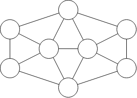
(a)

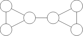
(b)

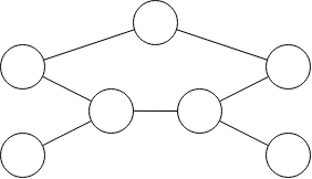
(c)

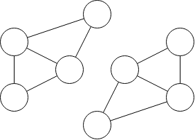
(d)

Figure 1: An undirected graph with induced and non-induced subgraphs. Fig. (a): The original undirected graph with 8 vertices and 15 edges. Fig. (b): An induced subgraph. Fig. (c): A non-induced subgraph. Fig. (d): A non-connected subgraph.

Given a graph $G=(V_{G},E_{G})$, a graph $H=(V_{H},E_{H})$ is a subgraph of graph $G$ (i.e., $H\subseteq G$) if it is composed by a set of vertices such that $V_{H}\subseteq V_{G}$. If $H$ includes all the edges $e\in E_{G}$ with both the endpoints in $V_{H}$, it is called an induced subgraph. Otherwise, $H$ is called a non-induced or partial subgraph. Fig. 1 shows some examples of induced and of non-induced subgraphs. Given two graphs, $G$ and $H$, the graph $S$ is a common subgraph if $S$ is simultaneously isomorphic to a subgraph of $G$ and to a subgraph of $H$.

A MCS of $G$ and $H$ is the largest possible common induced subgraph, i.e., the common subgraph with as many vertices as possible. Fig. 2 shows some examples with undirected and unlabeled graphs.

In the rest of the paper, we will indicate with $|V_{G}|$ and $|V_{H}|$ the number of vertices of $G$ and $H$, respectively.

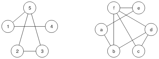
(a) Undirected graphs $G$ and $H$.

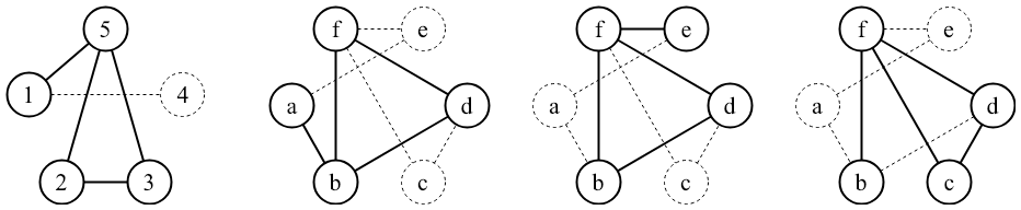
(b) Different MCS mappings for $G$ and $H$.

Figure 2: Given the graphs $G$ and $H$ represented in Fig. (a), Fig. (b) reports 4 different possible MCSs. Labels are shown only to help identify the vertices.

II-B The McSplit Algorithm

In 2017 McCreesh et al. [3] proposed McSplit, so far one of the most effective algorithm to find maximum common subgraphs. Different implementations of the algorithm are provided by the authors themselves, but essentially it is a recursive procedure based on two main ingredients: A smart invariant and an effective bound prediction formula.

The procedure dovetails together the two ingredients as follow. Let us suppose we have the two graphs $G$ and $H$ represented in Fig. 3(a) and 3(b). We consider graphs as simple as possible for the sake of readability. For now, we also suppose these graphs are undirected (even if they are represented as directed in Fig. 3) and unlabeled, i.e., the nodes labels $\{a,b,c,d\}$ are reported only to uniquely identify all vertices.

(a)

(b)

(c)

(d)

Figure 3: A running example. The graphs $G$ and $H$, of Fig. (a) and Fig. (b), produce the MCS of Fig. (c) if they are considered undirected and unlabeled, and the MCS of Fig. (d) if they are considered as directed and labeled.

McSplit builds a mapping $M$ between the vertices of $G$ and of $H$ using a depth-first search. At the very beginning $M$ is an empty set, and the algorithm adds a vertex pair to $M$ at each recursion level. During the first recursion step, let us suppose we arbitrarily select vertex $a$ in $G$, and we try to map this vertex with vertex $b$ in $H$, that is $M=\{a,b\}$. Now we label each unmatched vertex in $G$ according to whether it is adjacent to vertex $a$, and we label each unmatched vertex in $H$ according to whether it is adjacent to vertex $b$. For undirected graphs, adjacent vertex have label 1 and non-adjacent vertex have label 0. Table I(a) shows these labels. At this point, we recur and we try to extend $M$ with a new pair. A new pair can be inserted into $M$ only if the vertices within the pair share the same label. This is McSplit main invariant. If, during the second recursion step, we extend $M$ with pair $b$ and $c$, we obtain the new mapping $M=\{ab,bc\}$, and the new label set represented in Table I(b). The third step consists of extending $M$ with $c$ and $a$, which is, at this point, the only remaining possibility. We obtain $M=\{abc,bca\}$ and the label set of Table I(c). The last two vertex $d$ and $d$ cannot be inserted int $M$ because they have different labels. Then the recursive procedure backtracks and it looks-for another (possibly longer) match $M$. After all possibilities have been exhaustively explored, the final result, i.e., the MCS of $G$ and $H$ is represented in Fig. 3(c).

$G$		$H$			$G$		$H$			$G$		$H$
v	Label	v	Label		v	Label	v	Label		v	Label	v	Label
b	1	c	1		c	11	a	11		d	101	d	110
c	1	a	1		d	10	d	11
d	1	d	1

TABLE I: Labels on the non-mapped vertices of $G$ and $H$ with mapping: Fig. (a) $M=\{a,b\}$, Fig. (b) $M=\{ab,bc\}$. and Fig. (c) $M=\{abc,bca\}$.

As previously mentioned, the second very important ingredient of the algorithm is the bound computation. This computation is used to effectively prune the space search. While parsing a branch by means of a recursive call, the following bound is evaluated:

$$\small\begin{array}[]{ccl}bound&=&|M|+\sum_{l\in L}min(|\{v\in G:label(v)=l\}|,\\ &&\hskip 51.21495pt|\{v\in H:label(v)=l\}|)\end{array}$$ (1)

where $|M|$ is the cardinality of the current mapping and $L$ is the actual set of labels. If the bound is smaller than the size of the current mapping, there is no reason to follow that path along the tree search, as there is no possibility to find a match longer than the current one in there. In this way the algorithm prunes consistent branches of the decision tree, drastically reducing the computation effort.

As the MCS problem comes in many variants, McCreesh et al. propose small algorithmic variations to deal optimally with directed, vertex-labeled and edge-labeled graphs. For example, if we consider the graph in Fig. 3(a) and 3(b) as directed and with node labels, and we apply the previous process incrementing it with the two previous modifications, we find the MCS reported in Fig. 3(d).

III Parallel Approaches

In this section we present our parallel approaches, the CPU-based multi-core in Section III-A, and the GPU-based many-core in Section III-B.

III-A The CPU multi-core Approach

While Trimble himself briefly discusses a parallel multi-thread version to efficiently parallelize the algorithm analyzed in Section II-B [17, 18, 19], no complete description of the concurrent MCS function is available in the literature.

To implement the concurrent version of the algorithm, the original recursive procedure McSplit has been decomposed and restructured to balance the workload among the threads. The core delegates to a set of helper threads portions of the job done by the original function during its deeper recursion levels (fig. 4).

Figure 4: Partitioning the McSplit function to parallelize it.

The top-level function Solve orchestrates all worker threads. It initializes the matching process among vertices, and in order to achieve independence between working threads, it performs a copy of all relevant data structures, before moving into recursion. Depending on the recursion level, function Solve goes on calling a main thread or an helper thread.

The concurrency level has been tuned not to waste CPU-time copying data, and not overload the task queue in the thread-pool with too short tasks, avoiding slowdowns of the algorithm. During the first few levels of the recursion, each iteration of the main loop that pairs vertices from the two graphs is very time consuming; Then, the deeper in the recursion tree, the shorter become each branch. We define a threshold for the maximum depth in the recursion tree above which the function stops delegating work to other threads. Only main threads are called after the threshold. That is, delegation is not used when splitting the current task among more threads would be too expensive and would probably generate too many working threads.

Helper threads are called at lower recursion levels to help the main thread to solve its current task. It must be remarked that the main thread is not the first thread started by the operating system, and that in different phases of the algorithm, any thread can act as a main thread. Each thread executing the main function of a particular branch of the recursion, and eventually asking for help, acts as a main thread. At the same time, each thread helping a main thread acts as an helper thread.

In this scenario, threads cooperate with each other to compute, in parallel, different iterations of the main cycle in which pair of vertices are coupled depending on their labels. Thus the main task of all main threads and helper threads is to go on suggesting new matching pairs, and eventually recurring on their own recursion path. The main difference between main and helper threads is that the latter make a copy of all incoming data structure before moving on. The main and the helper functions are designed such that they are data-independent, and they can be assigned to different threads to be run in parallel. Anyway, they are actually linked by two atomic variables. The first one is used as a shared index of the main iterative construct. In this way, the main and the helper thread can execute the same cycle, but they must distribute iterations without both executing the same ones. The second atomic variable is the size of the current matching, which is shared among all threads to correctly evaluate the opportunity to proceed along a new path.

To further increase efficiency, all threads are kept running during the entire execution of the algorithm, and they are orchestrated using a thread pool. Such a pool implements a priority queue in which threads can insert the tasks they want to be helped with. These tasks include copies of the data structures and a pointer to the helper function. Helper threads can pick-up new tasks from the queue as soon as they are available. To achieve a higher level of parallelism, more than one helper thread can pick the same task and cooperate to solve it, also if at different times. The task objects are put in the queue following the order given by their position in the recursion three. For example, a task generated at depth $d$ will be put in the queue before any tasks generated at depth $d+1$. In the same way, a task generated at depth $d$ in the iteration $i_{n}$ of the main loop will be put after a task generated at depth $d$ in the first iteration $i_{0}$. The shared variables avoid repeating the same tasks more than once.

A simplify version of this entire process is represented by Algorithm 1. The top level procedure Parallel_McSplit receives the original graphs $G$ and $H$. It sets the current mapping $M$, and the best mapping $M_{best}$, to the empty set, and it initializes the priory queue $Q$ used by the thread-pool. After that, it calls function Solve which is essentially a recursive function adopting the concurrent scheme previously described. Solve receives as parameters the two graphs $G$ and $H$, the current and the best mapping $M$ and $M_{best}$, and the recursion level depth (properly initialize to 0). At each run of the recursive function, if a greater mapping has been found (lines 6–8). the best incumbent graph $M_{best}$ is updated. Then, the upper bound for the current search branch is computed (line 9) using Equation 1. If the bound has been hit (i.e., the current bound is lower or equal to the size of actual incumbent, thus no future search can improve it), the branch is pruned and the function returns (line 11). Otherwise, a new correct mapping is searched. In this case, first the most promising label class is selected from the remaining set of label classes (line 13), according to some heuristic. Then, a vertex belonging to that label class is selected as a new vertex $v$ (line 14).

Finally, the iterative cycle of lines 15–25 visits every vertex $u$ of $H$ belonging to the previously selected class. For each of these vertices, the recursive function explores the consequences to add the pair $(v,u)$, to the mapping (line 16). Notice that considering $(v,u)$ as a new pair in the mapping, implies splitting the current classes into two new sub-classes, according to whether vertices belonging to it are adjacent or not to $v$ and $u$. This operation if performed by function filterDomain at lines 17 and 18. At this point, as previously described, we resort to helper threads for the lower recursion levels (lines 20–21) and we proceed independently for higher depths (line 23). In the first case, a new pool task is first generated (line 20) and then enqueue in the thread pool queue (line 21). In the second case, a new recursive call is performed with updated $G$, $H$, $M$, $M_{best}$, and the recursion depth (line 23).

Notice that the process reported in lines 19–24 is repeated in lines 27–32. This last section of the code is required to check the case in which the vertex $v\in G$ is not mapped at all with any vertex of $H$. Thus $v$ is ruled-out from the graph $G$ (line 26) and the process proceeds either concurrently or recursively.

0:  

1:  $M$ = $\emptyset$

2:  $M_{best}$ = $\emptyset$

3:  QueueInit (Q)

4:  Solve ($G$, $H$, $M$, $M_{best}$, 0)

5:  QueueDestroy (Q)  

5:  

6:  if ($|M|>|M_{best}|$) then

7:     $M_{best}$ = $M$

8:  end if

9:  bound = computeBound ($G$, $H$, $M$)

10:  if (bound $\leq$ $|M_{best}|$) then

11:     return

12:  end if

13:  bidomain = selectLabelClass ($G$, $H$)

14:  $v$ = selectVertex (bidomain)

15:  for all $u\in H$ do

16:     $M=M\cup(v,u)$

17:     $\widehat{G}$ = filterDomain ($G$, $v$)

18:     $\widehat{H}$ = filterDomain ($H$, $u$)

19:     if (depth $\leq$ PART_LEVEL) then

20:        task = { $\widehat{G}$, $\widehat{H}$, $M$, $M_{best}$, depth }

21:        Enqueue (Q, Solve, task)

22:     else

23:        Solve ($\widehat{G}$, $\widehat{H}$, $M$, $M_{best}$, depth+1)

24:     end if

25:  end for

26:  $G=G\backslash v$

27:  if (depth $\leq$ PART_LEVEL) then

28:     task = { $G$, $H$, $M$, $M_{best}$, depth }

29:     Enqueue (Q, Solve, task)

30:  else

31:     Solve ($G$, $H$, $M$, $M_{best}$)

32:  end if

33:  return

Algorithm 1: The multi-core recursive branch-and-bound McSplit procedure.

As a last comment, notice that a fundamental role in the system is played by the queue within the thread pool and by the working threads running for the entire process and waiting for new tasks in the queue. In fact, the thread pool guarantees a very balanced work-load among threads: Any time a thread finishes a branch, it can go through the tasks queue and start helping other threads with their branches, thus reducing its idle time. This mechanism is not illustrated by the pseudo-code for the sake of simplicity, but depending of the status of the queue, various execution flow can be executed by threads:

• The task queue is empty. When the program starts and the thread pool is first initialized, each thread will start its own cycle when the task queue is empty. In this situation each thread acquires the lock on the queue (not everyone at the same time, of course), and then it tries to pick a task from the queue. Since the latter is empty, the thread skips all operations without doing anything, and the thread blocks on the condition variable waiting for someone to put a task in the queue and wake it up.

• Every time the Solve function adds a task to the queue, each thread of the thread pool that in that moment is waiting for the condition variable to become signalled is released. The first thread which manages to acquire the lock proceeds within its main cycle, and it picks the task from the queue. Even it this task should no longer be executed by any other thread, the only entity allowed to remove it from the queue is the one that put it in the queue.

• The task queue contains already executed tasks. The tasks queue is ordered by the position order of the tasks themselves, and thus tasks are executed and completed following the order of the recursion. Any completed task that is still being executed by some thread, will be at the beginning of the queue. When a task is executed it will be marked as such (if will have a NULL pointer instead of the actual pointer to the function which must solve the problem), such tasks will be simply skipped by any thread scanning the queue searching for a task to execute. When a task with a non-NULL pointer is found, the execution continues as the previous item point. If no task is found, the execution continues as in the first point.

III-B The GPU Many-core Approach

In this section, we show how the algorithm described in Section III-A can be modified in order to make it suitable to run on NVIDIA GPUs. We will concentrate on the most effective strategies and optimizations among the several different ones that have been implemented.

As shown in previous sections, McSplit is intrinsically recursive and the maximum recursion depth reached is equal to the size of the final solution graph. Unfortunately, even using Dynamic Parallelism, CUDA does not support more than $24$ in-depth recursion levels, and it is then suitable for graphs with a maximum of $24$ nodes. For this reason, the first step necessary to adapt the algorithm to CUDA, is to modify the execution structure in order to formally remove recursion. Substituting recursion explicitly using a stack is practically unfeasible on GPUs: First of all, as the stack would store every arguments for each virtual recursion, this approach would use a lot of memory and in an unpredictable way, whereas the memory for each thread memory on a GPU is quite limited. Moreover, each stack frame would correspond to a branch of the algorithm with its own varying depth, and the approach would lead to an extremely unbalanced workload on each GPU thread. In the next subsections, we analyze a few possibilities to decrease the algorithm memory usage and increase work-balance, while maintaining the absence of recursion.

III-B1 Labels re-computation

A first attempt is to get rid of the bidomain data structures and to drastically reduce the amount of information stored into the stack, is the following one. Each new stack entry consists of a pair of integers values. Each pair indicates a possible mapping between vertices of the two graphs. The current position in the final solution is stored into a proper variable, whose value is increased and decreased using two different special (and reserved) entries in the stack.

For example, let us suppose we are searching the MCS for two graphs ($G$ and $H$) with 5 vertices. At the beginning of the algorithm, any combination of one vertex from the first graph and one from the second graph is possible, and the stack will contain all those pairs, from $\langle 4,4\rangle$ down to $\langle 0,0\rangle$ (in reverse order, so they are popped out from the stack in the same order than the standard algorithm). When we pop the first pair, namely $\langle 0,0\rangle$, we also compute the new label classes for each remaining vertex from both the input graphs. Then, we must push in the stack all combinations of those pairs composed by vertices with matching labels. Anyhow, before pushing such pairs on the stack we push the pair $\langle-1,0\rangle$, and after pushing them we also insert the pair $\langle 0,-1\rangle$. In this way, when we pop the pair $\langle 0,-1\rangle$ we know that the current solution position is increased from 0 to 1. When we do that the algorithm starts popping pairs that it has to insert in the second position of the solution. At the same time, when the pair $\langle-1,0\rangle$ is extracted, the solution position returns to 0. Obviously, every time a better solution is found, it is stored in the incumbent solution, similarly to the standard algorithm.

Unfortunately, a fundamental aspect of this solution is that it does not allow to efficiently calculate the bound for a new branch. Indeed, every time a new pair is selected and inserted into the current solution, we must re-evaluate the labels for each remaining vertex to count the number of vertices with the same label we have, to finally compute the bound with Equation 1. Moreover, the necessity to store separately each vertex pair belonging to the same label class, instead of grouping them into a bidomain that is able to contain them all, leads to stack whose size is quickly increasing. These two drawbacks lead to massive slowdowns and make questionable its utilization in order to solve the problem in reasonable time.

III-B2 New bidomains stack

To recover from the drawbacks highlighted in the previous sub-section, our target is to group vertices in label-classes but keeping the stack small enough and maintaining the algorithm iterative.

To reach this target, we redesigned the stack to store bidomains data in an optimized form. New items are pushed into the stack every time a new set of bidomains is created, but they are popped out only after every pairs of vertices contained in the bidomains has been selected and explored. The stack thus become a matrix with eight columns, and a variable number of rows. Each column stores numbers representation at most the degree of the graph, thus we decided to use unsigned characters limiting the graphs size to $254$ vertices (the value $255$ is reserved by the algorithm). In this way each stack entry is four byte long, as in the previous implementation, in which each entry contained two integer values. Machines able to deal with graphs larger than $254$ vertices should also provide much more memory, so the same algorithm could be adjusted to work with unsigned integers too. Moreover, stack entries of eight bytes allow better memory alignment of the stack that can lead to benefits in memory performances and addresses calculation.

The first five values actually correspond to the ones included in the bidomain data structure with the same meaning (namely, left, right, left length, right length, and adjacent). The remaining three columns are used to store values that are necessary to restore values of certain variables when backtracking, as we need to explicitly store some values from previous iterations in the stack and we cannot resort to local variables within the recursive procedure.

Similarly, the current solution and the incumbent structure have been replaced by simple matrices of two rows and a variable number of columns, storing again unsigned characters.

Given this data structure, similarly to the standard algorithm, at each iteration of the main cycle, we choose a vertex from left bidomain and a vertex from right bidomain, then we put them in the solution and we compute the new bidomains depending on which vertices we just chose. However, in the recursive algorithm the selection of a vertex is performed by swapping it with the one at the end of the domain and by decreasing the bidomain size. In the recursive algorithm, this is possible because when backtracking to higher recursion levels, deep bidomains are destroyed, and the ones at higher levels has not been touched by lower recursions, thus the algorithm can continue with consistent data structures. When recursion is removed, however, we loose this important property, and when we select a vertex from the right bidomain and we decrease its size, the original size must be stored somewhere in order to be able to restore it when every right vertices has been tried with the selected left vertex. So we can select another left vertex and try again to pair it with every right vertex in the same bidomain. The values of the last column of the stack have precisely this purpose, every time a new bidomain is creates, is there stored the initial value of RL, for future utility.

In a similar way, we also need to recreate the behavior of the for loop of the recursive solve function, but since we have not a recursive call for each iteration, and the whole while main cycle is re-executed every time, we introduced an element in the stack that keep track every time of which right vertex has been selected, in order to correctly pick the next one.

Following this approach, every time a bidomain has been completely explored, we remove it from the stack and we pick the immediately following one. Doing so, we lose the possibility to choose which bidomain to select at each time. Indeed, such an approach, without any further optimization, performs significantly worse than the original on graphs larger than 15 nodes. However, it is pretty easy to implement a function to select a new label class similar to the original one. The idea, in this case, is to visit the stack backward (from top to bottom) to select the new bidomain following the desired heuristic and eventually exchange it with the one in the top of the stack.

IV The Portfolio Approach

The so-called “portfolio approaches” have been proposed and adopted in several domains. In such approaches, researchers drop the idea of designing a single, optimal algorithm, and resort to a portfolio of different tools, each one able to tackle specific instances of a given problem. The relationship between the properties of a problem instance and tool’s performance is typically opaque and difficult to capture, the construction of a portfolio normally involves machine-learning activity.

Portfolio approaches were demonstrated the best approach for model checking and satisfiability in recent competition contexts [20, 4, 5]. In these scenarios, portfolio approaches have often been used in order to emphasize multi-core CPU exploitation, and to encourage multi-threaded solutions [21]. Moreover, portfolio approaches have been proved to be more diversified, and less sensitive to model characteristics [22, 23, 24].

Generally speaking, portfolio tools take as input a distribution of problem instances and a set of tools, and constructs a portfolio, optimizing a given objective function. The function can be related to the mean runtime, percent of instances solved, or score in a competition. In our case, we will focus on the number of instances solved in a specific slotted wall-clock time. Using wall-clock time versus using only process time, both as time limit and for tie-breaking, has the advantage to encourage parallelization of tools. Indeed, the concurrency level of each tool can often be guessed only from experimental data, comparing CPU and wall-clock run times. Furthermore, in our portfolio, we may not only have different solvers possibly running in parallel on the CPU cores, but at least one version running on the GPU, thus augmenting the range of variations and affecting different hardware devices, with separate resources.

We built our portfolio starting with the following code versions:

• Versions ($mc1$ and $mc2$), are the original versions (sequential and parallel, respectively) implemented by McCreesh et al. [3], in C++.

• Version 1 ($v1$) is a sequential re-implementation of the original code in C language. This code constitutes the starting version for all our implementations, as it is more coherent with all following requirements, modifications, and choices.

• Version 2 ($v2$) is the C multi-thread version described in Section III-A. It logically derives from $mc1$ and $v1$.

• Version 3 ($v3$) is an intermediate CPU single-thread implementation that removes recursion and decreases memory usage. It is logically the starting point for comparison for the following two versions.

• Version 4 ($v4$) is a CPU multi-thread implementation based on the same principles of the following CUDA implementation.

• Version 5 ($v5$) is the GPU many-thread implementation, described in Section III-B. It is based on $v3$ and $v4$.

In the sequel, we will refer to the portfolio tool itself with $vP$. Notice that while the original version $mc1$ and $mc2$ were written in C++, all our versions have been written in C language but $v5$ which is written in CUDA. Note that versions $v3$ and $v4$ have been developed to explore the feasibility of new approaches in developing a maximum common subgraph algorithm in CUDA environment, not to obtain the best possible performances. For example, $v4$ is drastically slower than all other versions, but it represents the possibility to run the algorithm implemented in version 3 on more threads, which are completely independent from one another. Indeed the same system is used on a wider scale in version 5, which is significantly faster than $v4$, although they make use of the same approach.

We also consider the clique encodings of McCreesh et al. [25], and the k$\downarrow$ algorithm of Hoffmann et al. [26]. To increase the range of variations we also modified versions $v2$, $v3$, and $v5$ as described in the following section.

IV-A Portfolio-based Modifications

An efficient branch-and-bound procedure requires a good initial ordering to rearrange the recursion tree and improve the convergence speed. We propose an approach based on the analysis and permutation of the adjacency matrix of the two graphs to produce good recursion trees, which may significantly affect the time and memory requirements of the computation. When ordering an adjacency matrix for graph isomorphism, the rows of the matrix correspond to a permutation of the initial pairing scheme. We assume that the order is top-down. A straightforward analysis suggests that it is advantageous to pair variables with similar support sets. Mc Creesh et al. [3] always sort the vertices in descending order of degree (or total degree, in the case of directed graphs). Anyhow, as the same authors noticed, some improvements is possible in that direction.

In mathematics, a block matrix is a matrix that can be partitioned into a collection of smaller matrices each one including a block of horizontal and vertical lines. If we consider the adjacency matrix of a directed graph, the presence of more than one connected component in the graph signals the existence of non-trivial block-diagonal form for the matrix. Identifying the connected components of the graph and then ordering each component individually is desirable. Finding the connected components is linear in the size of the matrix, even for full matrices, and leads to decomposition of the problem. The overall order for a matrix that has multiple connected components is obtained by concatenating the orders for each component. The sorting of the components is based on the ratio of number of rows to number of columns. If the ratio is large, the component goes toward the beginning of the schedule.

Within each component, we order the vertices based on their bit relations. A square matrix is called upper triangular if all the entries below the main diagonal are zeros. Our ordering procedure is roughly based on the algorithm of Hellerman and Rarick [27] to put a matrix in bordered block lower-triangular form. Initially, all non-zero rows and columns of the matrix block form the active submatrix. The procedure then iteratively removes rows and columns from the active block submatrix and assigns them to final positions. It iteratively chooses the column that intersects the maximum number of shortest rows of the active submatrix. Then, it moves that column out of the active block submatrix and immediately to its left. Once the active block submatrix vanishes, the block matrix has been permuted.

As analyzes in Section II-B the recursive procedure adopts a quite effective bound prediction formula to constrain the tree search. However, this constraining effect is reduced when the value of the current bound gets closer to the actual one. Moreover, repeated adjustments of the bound may drastically slow-down the procedure, forcing it to visit useless tree sub-sections. For this reason function McSplit was also modified using a top-down strategy (similar to the one adopted by k$\downarrow$ [26]) by calling the main solve function once per goal size, that is, $|V_{G}|$, $|V_{G}|-1$, $|V_{G}|-2$, etc., being $G$ the smaller graph between $G$ and $H$. This procedure has been proved to beat the original ones in those cases in which the MCS covers nearly all of the smaller graph.

Moving in this direction, Fig. 5(b) shows the cost of procedure $mc1$ (the original sequential version of McSplit) as a function of size of the computed MCS. For the sake of simplicity, we consider only one representative graph pair with increasing size of the MCS, size varying from $15$ to $25$. Essentially, the two plots report the number of recursions (Fig. 5(a)) and the wall-clock times (Fig. 5(b)) required to move from one value of the bound to the next one. As we use a logarithmic scale along the y-axis, it is easy to infer that costs drastically increase with the bound, and get quite high close to the final bound value.

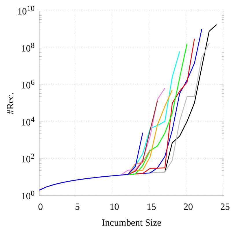
(a)

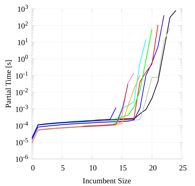
(b)

Figure 5: Number of recursions (a) and wall-clock times (b), in the standard sequential MsSplit procedure, as a function of the size of the MCS discovered.

Keeping this consideration in mind, we define “dead-ends” the condition in which no larger MCS is found, but the branch-and-bound procedure keeps recurring. Dead-ends re-computation may prove expensive, and we try to forecast them and to reduce their impact. To predict dead-ends, we rely on a global criterion such as the number of recursions. When this number exceeds a specific threshold without improving the size of the minimum common subgraph, we consider the current sub-tree as leading to a dead-end. Threshold can be evaluated using absolute values or by taking into consideration the number of recursions that led to the last increment of the bound. Once a dead-end is forecast, we experimented with two different alternatives to reduce its impact.

The first one consists in increasing the bound either by a little value (usually $1$), or by doubling it. After varying the bound the procedure may prove that the new bound is till reachable, finding a higher bound, or unreachable, proving unable to find a higher bound. In the first case, we have just avoided several useless iterations, pruning the search tree much faster and increasing the convergence speed. In the second one, we have found an upper bound for the size of the MCS. In this case, we look for the correct bound exploiting a binary search within the lower and the upper bounds. This search converges in a logarithmic number of recursive checks to the exact bound.

A second possibility consists in adopting a “restart” strategy. Restart strategies have been proposed for satisfiability (SAT) solvers, and they have been used for over a decade [28]. With a restart a SAT solver is forced to backtrack according to some criterion. Although, this may not be considered as a sophisticated technique, there is mounting evidence that it has crucial impact on performance. In our case, restarting can be thought of as attempt to avoid spending too much time in branches in which there is not an MCS larger than the current one. We adopt a simple restart strategy for our MCS tools, consisting in the random selection of the another tree branch within the current bidomain representation, from which to move on using recursion. At the same time, to make sure that the branch-and-bound procedures stop searching only once the entire tree has been visited, for each restart we store global information to indicate which part of the tree has already been visited. This information consists of task object pairs. Task objects have been introduced in Section III-A, and each pair indicates the range of recursions already taken into consideration. Notice that, to avoid too large data structure and to be efficient, restarts should not be applied too frequently. As a consequence, in this case we often trigger a new restart when the number of recursions has doubled with respect to the last one in which we found a larger MCS.

In our implementation, all previous engines are orchestrated by a a Python interface. This interface may run in two modalities. In the first one, a number of processes, each one running a different algorithm or a different configurations of the same algorithms, are run in parallel. Whenever a process finishes with a result all others are terminated. In the second one, we first run only sequential versions for a few seconds (usually from 5 to 10). In case a results is not returned, we concurrently run the parallel CPU and massively parallel GPU versions. In this last case, the CPU and the GPU versions proceed independently, even if some information (e.g., the current bound) could be maintained and updated globally. The portfolio thus include several tool versions written in C, C++, and CUDA, plus an high-level script written in Python. We will refer to the portfolio version as version $vP$ in the sequel.

V Experimental Results

In this section we report results for all versions described in Section IV (with and without the modifications reported in Section IV-A), plus the multi-engine (portfolio) application ($vP$).

Tests have been performed on a machine initially configured for gaming purposes and equipped with a CPU Intel i7 4790k over-clocked to 4.4 GHz; 16 GiB of RAM at $2,133$ MHz; a GPU NVIDIA GTX 980 over-clocked to 1,300 MHz, with 4 GiB of dedicated fast memory and 2,048 CUDA cores belonging to Compute Level 5.2. The CPU has 4 physical cores, which benefit from Intel’s Hyper-Treading and are split into 8 logical cores, theoretically improving multitasking. The number of threads present in the pool for the parallel CPU version is set to the number of logical threads that can run in parallel on the processor, i.e., 8. The operating system used was Ubuntu 18.04 LTS.

V-A Data-sets description

We tested our code using the ARG database of graphs provided by Foggia et al. [8] and De Santo et al. [7]. The ARG database is composed by several classes of graphs, randomly generated according to six different generation strategies with various parameters settings. The result is a huge data-set of 168 different types of graphs and a total of $166.000$ different graphs.

For our purposes, we selected only a subsection of the data-set, containing graphs pairs already prepared to have maximum common subgraphs of specific dimension. In particular we used the mcs10, mcs30, mcs50, mcs70 and mcs90 categories, i.e., graphs pairs with maximum common subgraphs corresponding to 10, 30, 50, 70 and 90% of the original graphs size. For each of these categories several generation strategies are present, such as bound-valence graphs (bvg) or graphs generated using 2D, 3D or 4D meshes with different parameters.

Starting from this subset of the ARG database we considered two sub-categories of graphs pairs: Small ones (with less than 40 vertices, 2,750 pairs), and medium (from 40 to 50 vertices, 240 pairs). Graphs larger than 50 vertex are not considered as it has been impossible to solve any problem in less than 1,000 seconds. All graphs are manipulated as undirected and unlabelled to generate the following results.

V-B Analysis of the Stand-Alone Procedures

Fig. 6 plots all tested versions on the small graph set with a tight wall-clock time limit, equal to 10 seconds. Given an execution time threshold on the x-axis, the relative y value indicates the number of problem instances solved by the algorithm under such a threshold. The x-axis has a logarithmic scale, while the y-axis is standard linear. For instance, from the $mc2$ plot, we can read that the parallel C++ version solved just over 2,000 instances (out of 2,750) in less than $10^{-1}$ seconds. The sequential version took about four times the time to solve the same number of instances.

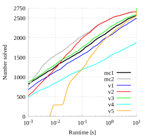
Figure 6: Cumulative number of instances (y axis) solved in under a certain time (x axis).

Not surprisingly, multi-threaded versions are usually less effective for very small problems. This is mainly due to the higher computing overhead for threads instantiation. As a consequence, none of the multi-thread versions can be considered faster than any sequential version to solve small and easy instances. Nevertheless, starting from run-times around $10^{-3}\div 10^{-2}$ seconds, parallels version quickly recover the performance gap and actually start performing significantly better for every remaining instances, with speedups up to almost an order of magnitude.

It is also clear that the sequential version ($v3$) performs more or less as the corresponding recursive version. On the contrary, the multi-thread iterative version ($v4$) is actually the worst performing version of the group. This fact can be explained by remembering that such version was only developed to explore the possibility to implement the sequential algorithm in a multi-thread but non-collaborative way. Thus threads in this implementation are independent, and performances can better scale by increasing the number of threads, what is desirable attempting a CUDA implementation.

As expected, due to the high computing overhead necessary to initialize the environment, the CUDA version is significantly slower than any other to start. You can also clearly see that the plot has a flat step in the bottom part. This phenomena is due to the fact that the algorithm runs on the CPU up to the fifth depth level of the virtual research tree and only after such level branches are delegated to GPU threads. In any instance for which the solution turns out to be very small (i.e., a maximum common subgraph with up to 5 vertices), actually the GPU is never called into play, and the computation is entirely done by the CPU. Such instances, in the small set database are about $260$, and they are the first growing part of the plot, up to the step. Then when instances begin to have larger solutions, and thus also the GPU is used to solve them, a gap is formed due to the need of copying data to and from the GPU. For this reason instances that make use of the GPU can not run for less than about $20$ milliseconds, and this determine the gap in the graphic. From there on, performances increases much faster than any other version, actually going to almost equalize CPU parallel versions in number of timeout instances, even with a much slower start.

For the smaller set parallel CPU versions (both the original one in C++ and our C implementation) are the best performing implementations. The CUDA implementation, even if not competitive for very easy instances, is faster then the C sequential versions for run-times higher than one second. Moreover, for the harder instances, CUDA is able to close the gap with the faster implementations, and it can be noted that the tangent line to the curves in the timeout point, at 10 seconds, is almost horizontal for the original parallel versions, while it is more inclined for the CUDA one. This let us imagine that for harder instances, i.e., requiring more than $100$ seconds, the CUDA implementation could become faster than all other implementations.

Fig. 7 plots separately sequential and parallel versions. From Fig. 7(a) it is possible to see that all sequential versions perform more or less in the same way, with a gap of about half an order of magnitude between the slowest and the fastest version. It is interesting to notice that for the sequential approach, the iterative approach is the fastest one. A different situation is shown in Fig. 7(b) where the iterative multi-thread version performs up to two orders of magnitude worse than the original parallel versions. Moreover, it is possible to notice that the parallel C++ version performs generally better for instances of simpler and medium difficulty.

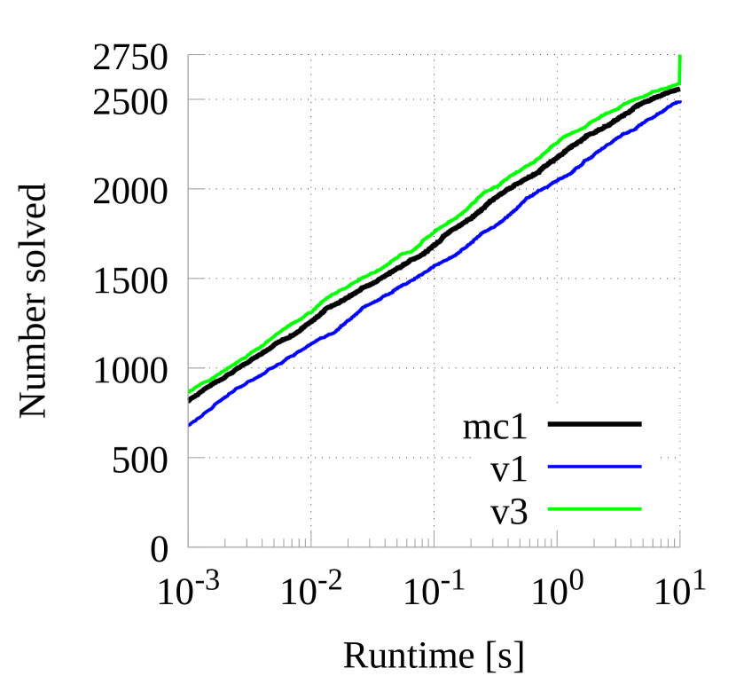
(a) Sequential summary.

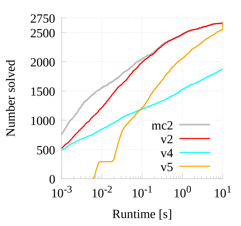
(b) Multi-thread summary.

Figure 7: Cumulative number of instances (y-axis) solved in under a certain time (x-axis) plotted separately for the sequential and parallel versions.

Fig. 8 reports the plots for the small and the medium graph sets considered together. The allowed wall-clock time has been increase to $1000~{}s$. In this picture, we just consider the fastest strategies of Fig. 6. As it can be noticed, as previously imagined, the CUDA version closes the gap with the parallel CPU implementation around $20$ seconds, and it is definitively faster than the CPU version up to about $400$ seconds.

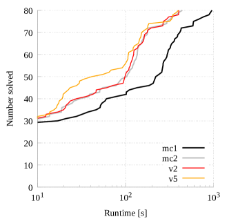
Figure 8: Cumulative number of instances solved in a given runtime by the fastest CPU versions ($mc1$, $mc2$ and $v2$) and by the GPU ($v5$) implementation.

Two main aspects influence the performances of our CUDA implementation. They are the principle of data locality and the branch divergence. The first one needs to be maximized, so that when threads in the same warp access a variable in their local memory, all requests can be grouped in one single memory fetch of consecutive memory locations. In this way, the kernel better use the memory bandwidth. The second aspect, needs to be minimized. In fact, when threads in the same warp hit a branch instruction and they take different routes, the whole warp execute both the routes sequentially, with part of the treads stalling for the first route and part of the threads stalling for the second ones. In this way the different branch paths are not executed in parallel but sequentially, and their execution time is added up. Moreover, if one or a few threads take a significantly longer route, compared to any other thread, during the same kernel execution, it or they will necessarily be waited by every other thread. Fig. 9 represents an analysis of the main reasons forcing our working threads in a stall situation.

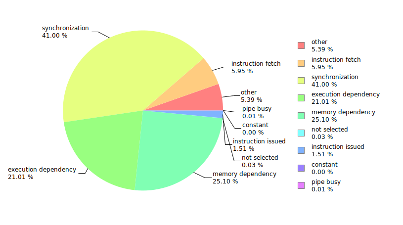
Figure 9: The chart represents all main reasons forcing the CUDA kernel function to stall, decreasing performances.

Three main reasons can be easily identified: Synchronization, memory dependency, and execution dependency. Synchronization issues, with $41$% of the overall stalls, happen when a thread is blocked on a __syncthreads instruction. Unfortunately, for the McSplit algorithm the workload for different threads is inherently heavily unbalanced. Thus many of them stall at the end of their execution, just waiting that slower threads finish their work before finding the current best solution found during the kernel execution. The second main reason for stalling, i.e., the memory dependencies, is due to those cases in which a load or store operation needs to wait for free memory bandwidth. This situation happens quite frequently in our code, where the data locality principle is limited, because each thread has a separate stack to simulate recursion, and the stack is allocated in the local memory of each thread. Thus, every time a location of the stack is accessed, a memory fetch has to be performed, and such requests cannot be coalesced within threads in the same warp, because each threads access to different cells of respective stack that are not close in memory. The third significant for thread stalling, i.e., execution dependency, happens when an instruction is stalled waiting for one or more arguments to be ready. This problem can be avoided by increasing instruction-level parallelism, but of course improving it is not that simple, because we also have to take into account the number of registers reserved for each thread, and the one available for each block. This is an important limitation to increase the number of threads and the instruction parallelism.

In addition to the stalls chart, it is also interesting to observe that some branch instructions in the kernel function show an high amount of divergence during the execution. Fig. 10 indicates the most divergent instructions inside the body of the kernel function discovered by Nsight. Note that the worst one, the one at line $325$, corresponds to the branch where the bound of the current branch is computed and the branch is eventually pruned. When the tree branch is not pruned, the body of the main loop of the kernel function is executed to compute new label domains and new solutions. On the contrary, when the branch is pruned, the code jump to the next main iteration. The overall behavior is then significantly different. All other relevant branches with high divergence (around $20$%), are again inside the main loop of the kernel function. This lead to overall high percentage of branch divergence in the core of the kernel function, limiting a lot the maximum instruction throughput reachable by the kernel.

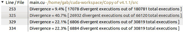
Figure 10: Extract from the profiling analysis executed by Nsight. The analysis shows the most divergent instructions in our CUDA main code section.

V-C Analysis of the Portfolio Approach

We insert in our portfolio the versions of the MCS procedure described in Section IV. Versions $v2$, $v3$ and $v5$ have also been augmented with the heuristics and the settings described in Section IV-A.

To analyze the potential benefit of our portfolio approach, Fig. 11 compares the performance of the original version $v3$ modified with 3 different heuristics. These settings include our reordering strategy for the adjacency matrix, our dead-end prediction with bound correction, and the dead-end prediction with randomize restart. The 3 plots report the running times for the original (reference) version on the x-axis, whereas they represent with different symbols (and colors) the running times for the 3 modified versions. Points on the main diagonal include benchmarks on which the performance is the same. Fig. 11(a) focuses on small graph pairs which can be solved within 2 seconds, Fig. 11(b) concentrates on a time range up to 10 seconds, and Fig. 11(c) extends the analysis to 500 seconds. As it can be noticed, different heuristics perform quite differently on different graph pairs even if they do not really improve the original version on average. For example, in the time range fro 0 to 10 seconds, the original version $v2$ is the fastest method in 34% of the cases, whereas the 3 heuristics make it faster in 26%, 23%, and 13% of the cases, respectively (all versions run out of time in the remaining 4–5% of the cases). Similar considerations hold for the procedures described in Section IV. A more accurate analysis of the the data plotted in Fig. 6 show that the number of instances on which the various methods are the fastest ones are the following: $mc1$ 60, $mc2$ 1404, $v1$ 10, $v2$ 245, $v3$ 947, $v4$ 0, and $v5$ 4. The same conclusions can be derived from the cumulative plot if Fig. 8, as the CPU and the GPU procedures have similar performance on average, but they present quite different performance on a benchmark-by-benchmark basis.

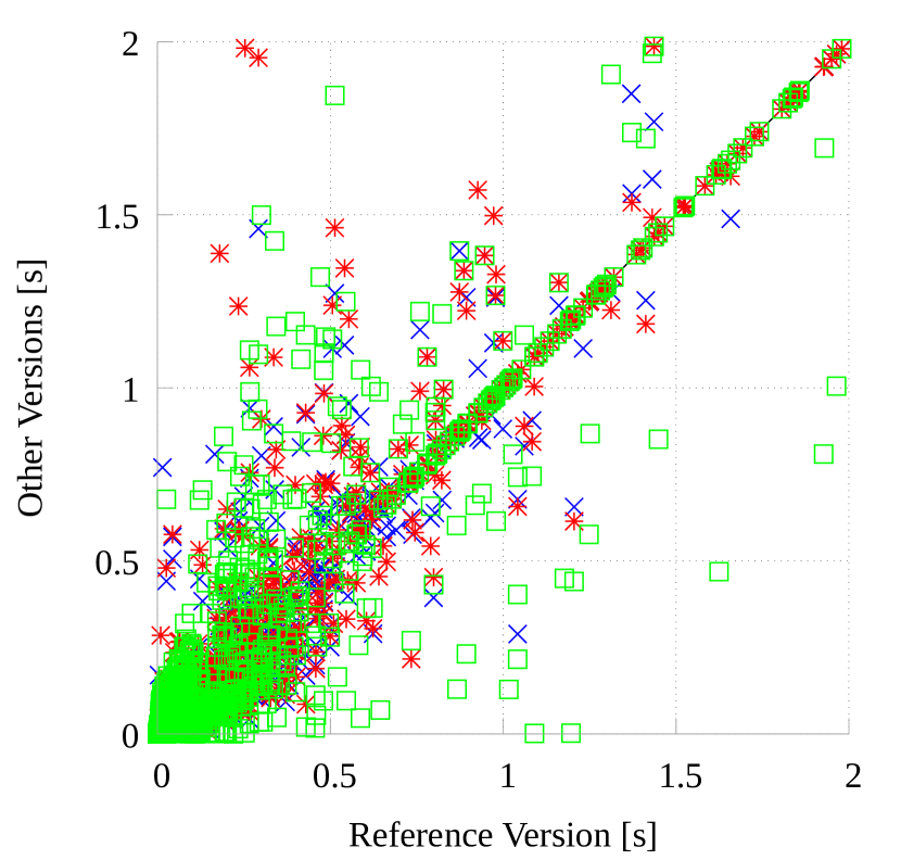
(a)

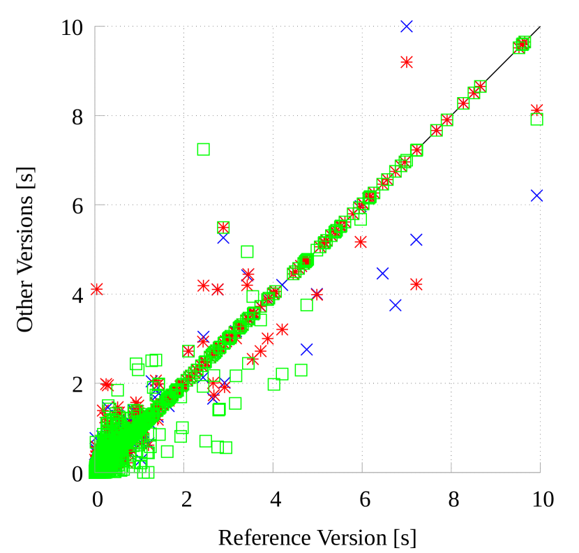
(b)

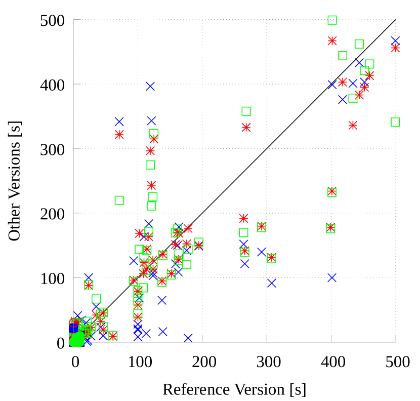
(c)

Figure 11: Running times for different heuristics (reported on the y-axis) implemented within the sequential version (reported on the x-axis) denoted as $v3$ and taken as reference version. These heuristics include the reordering strategy for the adjacency matrix (blue crosses), the dead-end prediction with bound correction (red stars), and the dead-end prediction with randomize restart (green boxes). Plots 11(a), 11(b), and 11(c) focus on different time ranges, i.e., 0–2, 0–10, 0-500 seconds.

Results gathered with the portfolio approach are presented in Fig. 12. The two graphics plot the most efficient approaches (as represented if Fig. 6 and Fig. 8) with the one gathered with our portfolio ($vP$). As in the previous cases, Fig. 12(a) includes data for small graphs analyzed up to 10 seconds. Fig. 12(b) extends our analysis for medium graphs. and a time limit up to 1000 seconds. It is easy to argue that the portfolio is faster on average and able to solve more instances that any other method on both wall-clock time (and graph size) ranges.

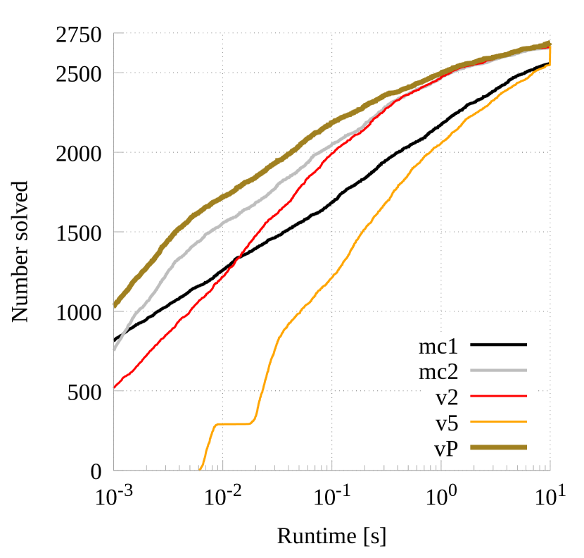
(a)

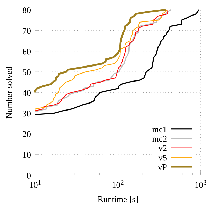
(b)

Figure 12: The most efficient sequential and parallel McSplit versions compared against the portfolio with a time limit of (a) $10$ seconds and (b) $1,000$ seconds.

VI Conclusion

In this work, we extend the algorithm named McSplit, a state-of-the-art branch-and-bound algorithm to find the maximum common subgraphs between two graphs.

First, we parallelize it, both to as a multi-core CPU implementation and as a CUDA-based GPU many-core one. Concerning the CPU procedure, we experimented with several parallel approaches, going from using different data structures to adopting several divide-and-conquer paradigms, with the purpose of balancing the threads workload and to keep under control the memory usage. As far as the CUDA extension is concerned, the main issue is that, like many other graphs algorithms, the analyzed one is based on complex data structures and on recursion. Both features do not usually suit well with GPU computing, and we propose a few ways to overcome these limitations.

Then, we develop new heuristics to reorder the adjacency matrix, trying to isolate matrix blocks and make them upper triangular, to smooth the heavy-tail phenomenon dealing with dead-ends, and to restart the process with automatic restarts. These algorithms, albeit not more efficient than the original ones from an average point of view, allow a significant performance improvement for specific graph pairs.

Finally, we propose a portfolio approach, integrating several local search algorithms as component tools. In this portfolio, a python interface orchestrate many CPU versions with one GPU procedure, exploiting modern hardware resources at their best. We demonstrate that the portfolio approaches is beneficial in the domain, and CUDA versions may worth further analysis.

Andrea Marcelli received his M.Sc. degree in Computer Engineering from Politecnico of Torino, Italy, in 2015. Currently he is a Ph.D. student in Computer and Control Engineering at the same institute and member of the CAD group. His research interests include malware analysis, semi-supervised modeling, machine learning and optimization problems, with main applications in computer security.

Stefano Quer received a M.S. in Electronic Engineering from Politecnico di Torino in $1991$, and a Ph.D. degree in Computer Engineering, from the Ministry of University and Scientific and Technological Research in Rome in $1996$. He has been a Visiting Faculty in the Department of Electronic Engineering and Computer Science of the University of California in Berkeley. He has been an intern with the “Advanced Technology Group” at Synopsys Inc., Mountain View, California, and with the “Alpha Development Group” at Compaq Computer Corporation, Shrewsbury, Massachussetts. He has been a Compaq Computer Corporation consultant. He is currently professor with the Department of Control and Computer Engineering at Politecnico di Torino, Torino, Italy. His main research interests include systems and tools for CAD for VLSI, formal methods for hardware and software systems, and embedded systems. Other activities focus on the development of sequential and concurrent algorithms and on optimization techniques able to achieve acceptable solutions with limited resources.

Giovanni Squillero (M01-SM14) received his M.S. and Ph.D. in computer engineering in 1996 and 2001, respectively. He is currently an associate professor of computer science at Politecnico di Torino. His research mixes the whole spectrum of bio-inspired metaheuristics with computational intelligence, machine learning, and selected topics in electronic CAD, games, multi-agent systems. Other activities focus on the development of optimization techniques able to achieve acceptable solutions with limited amount of resources, mainly applied to industrial problems.

References

- [1] H. G. Barrow and R. M. Burstall, “Subgraph isomorphism, matching relational structures and maximal cliques,” Inf. Process. Lett., vol. 4, no. 4, pp. 83–84, 1976.
- [2] C. Bron and J. Kerbosch, “Finding all cliques of an undirected graph (algorithm 457),” Commun. ACM, vol. 16, no. 9, pp. 575–576, 1973.
- [3] C. McCreesh, P. Prosser, and J. Trimble, “A partitioning algorithm for maximum common subgraph problems,” in Proceedings of the 26th International Joint Conference on Artificial Intelligence, ser. IJCAI’17. AAAI Press, 2017, pp. 712–719. [Online]. Available: http://dl.acm.org/citation.cfm?id=3171642.3171744
- [4] “The SAT Competition Web Page,” http://www.satcompetition.org/, accessed: 2014-12-01.
- [5] “The SMT Competition Web Page,” http://www.smtcomp.org/, accessed: 2014-12-01.
- [6] L. Kotthoff, C. McCreesh, and C. Solnon, “Portfolios of subgraph isomorphism algorithms,” in Learning and Intelligent Optimization, P. Festa, M. Sellmann, and J. Vanschoren, Eds. Cham: Springer International Publishing, 2016, pp. 107–122.
- [7] M. De Santo, P. Foggia, C. Sansone, and M. Vento, “A large database of graphs and its use for benchmarking graph isomorphism algorithms,” Pattern Recogn. Lett., vol. 24, no. 8, p. 1067–1079, May 2003. [Online]. Available: http://dx.doi.org/10.1016/S0167-8655(02)00253-2
- [8] P. Foggia, C. Sansone, and M. Vento, “A database of graphs for isomorphism and sub-graph isomorphism benchmarking,” in -, 2001, p. 176–187.
- [9] H. Bunke, P. Foggia, C. Guidobaldi, C. Sansone, and M. Vento, “A comparison of algorithms for maximum common subgraph on randomly connected graphs,” in Joint IAPR International Workshops on Statistical Techniques in Pattern Recognition (SPR) and Structural and Syntactic Pattern Recognition (SSPR). Springer, 2002, pp. 123–132.
- [10] D. Conte, P. Foggia, and M. Vento, “Challenging complexity of maximum common subgraph detection algorithms: A performance analysis of three algorithms on a wide database of graphs.” J. Graph Algorithms Appl., vol. 11, no. 1, pp. 99–143, 2007.
- [11] P. Vismara and B. Valery, “Finding maximum common connected subgraphs using clique detection or constraint satisfaction algorithms,” in Modelling, Computation and Optimization in Information Systems and Management Sciences. Springer, 2008, pp. 358–368.
- [12] M. Minot and S. N. Ndiaye, “Searching for a maximum common induced subgraph by decomposing the compatibility graph,” in en. In: Bridging the Gap Between Theory and Practice in Constraint Solvers, CP2014-Workshop, 2014, pp. 1–17.
- [13] A. C.-L. Chen, A. Elhajj, S. Gao, A. Sarhan, S. Afra, A. Kassem, and R. Alhajj, “Approximating the maximum common subgraph isomorphism problem with a weighted graph,” Knowledge-Based Systems, vol. 85, pp. 265–276, 2015.
- [14] H. Bunke, P. Foggia, C. Guidobaldi, and M. Vento, “Graph clustering using the weighted minimum common supergraph,” in Proceedings of the 4th IAPR International Conference on Graph Based Representations in Pattern Recognition, ser. GbRPR’03. Berlin, Heidelberg: Springer-Verlag, 2003, pp. 235–246. [Online]. Available: http://dl.acm.org/citation.cfm?id=1757868.1757895
- [15] V. Blondel, A. Gajardo, M. Heymans, P. Senellart, and P. Van Dooren, “A measure of similarity between graph vertices: Applications to synonym extraction and web searching,” SIAM Review, vol. 46, no. 4, pp. 647–666, 2004. [Online]. Available: https://doi.org/10.1137/S0036144502415960
- [16] L. A. Zager, “Graph similarity and matching,” Ph.D. dissertation, Massachussetts Institute of Technology, USA, 2005. [Online]. Available: http://hdl.handle.net/1721.1/34119
- [17] J. Trimble, “Mcsplit implementations,” https://github.com/ciaranm/cpaior2018-parallel-mcs-paper/tree/master/james-cpp-parallel, 2017.
- [18] C. McCreesh, “Solving hard subgraph problems in parallel,” Ph.D. dissertation, University of Glasgow, 2017.
- [19] R. Hoffmann, C. Mccreesh, S. N. Ndiaye, P. Prosser, C. Reilly, C. Solnon, and J. Trimble, “Observations from parallelising three maximum common (connected) subgraph algorithms,” in International Conference on the Integration of Constraint Programming, Artificial Intelligence, and Operations Research. Springer, 2018, pp. 298–315.
- [20] G. Cabodi, C. Loiacono, M. Palena, P. Pasini, D. Patti, S. Quer, D. Vendraminetto, A. Biere, and K. Heljanko, “Hardware Model Checking Competition 2014: An Analysis and Comparison of Model Checkers and Benchmarks,” vol. 9, pp. 135–172, jun 2016.
- [21] L. Bordeaux, Y. Hamadi, and H. Samulowitz, “Experiments with massively parallel constraint solving,” in IJCAI, 2003.
- [22] L. Xu, F. Hutter, H. H. Hoos, and L. Leyton-Brown, “SATzilla: Portfolio-based Algorithm Selection for SAT,” Journal of Artificial Intelligence Res., vol. 32, no. 1, pp. 565–606, 2008.
- [23] L. Pulina and A. Tacchella, “A self-adaptive multi-engine solver for quantified boolean formulas,” Constraints, vol. 14, no. 1, pp. 80–116, Mar 2009. [Online]. Available: https://doi.org/10.1007/s10601-008-9051-2
- [24] Y. Hamadi and L. Sais, “Manysat: a parallel sat solver,” JOURNAL ON SATISFIABILITY, BOOLEAN MODELING AND COMPUTATION (JSAT), vol. 6, 2009.
- [25] C. McCreesh, S. N. Ndiaye, P. Prosser, and C. Solnon, “Clique and constraint models for maximum common (connected) subgraph problems,” in International Conference on Principles and Practice of Constraint Programming. Springer, 2016, pp. 350–368.
- [26] R. Hoffmann, C. McCreesh, and C. Reilly, “Between subgraph isomorphism and maximum common subgraph,” in Thirty-First AAAI Conference on Artificial Intelligence, feb 2017, p. 3907–3914.
- [27] S. Hellerman and D. C. Rarick, “The partitioned preassigned pivot procedure (p4),” Sparse Matrices and Their Applications, vol. 67-76, 01 1972.
- [28] C. P. Gomes, B. Selman, and H. Kautz, “Boosting combinatorial search through randomization,” in Fifteenth National/Tenth Conference on Artificial Intelligence/Innovative Applications of Artificial Intelligence, ser. AAAI ’98/IAAI ’98. Menlo Park, CA, USA: American Association for Artificial Intelligence, 1998, pp. 431–437. [Online]. Available: http://dl.acm.org/citation.cfm?id=295240.295710