On a progressive and iterative approximation method with memory for least square fitting

Abstract

In this paper, we present a progressive and iterative approximation method with memory for least square fitting (MLSPIA). It adjusts the control points and the weighted sums iteratively to construct a series of fitting curves (surfaces) with three weights. For any normalized totally positive basis even when the collocation matrix is of deficient column rank, we obtain a condition to guarantee that these curves (surfaces) converge to the least square fitting curve (surface) to the given data points. It is proved that the theoretical convergence rate of the method is faster than the one of the progressive and iterative approximation method for least square fitting (LSPIA) in [Deng C-Y, Lin H-W. Progressive and iterative approximation for least squares B-spline curve and surface fitting. Computer-Aided Design 2014;47:32-44] under the same assumption. Examples verify this phenomenon.

1 Introduction

Least square fitting to a set of data points by a parametric curve or surface is a fundamental problem in Computer Aided Geometric Design [1, 2] and a well-known key technology in many application areas. It is powerful especially when dada set is very larger.

Based on different metric descriptions, there are two main kinds of least square fittings. One is to take control points and parameter knots as variables, so that nonlinear least square problems should be solved. Since it is nonlinear, a proper initial fitting need. The other one is to assign a parameter for each data point, so that the data set becomes organized. In this case, linear least square fittings need to be solved to obtain control points. Since it is linear, the construction of the method may be simpler. One can look for more details about these two kinds of fittings, for examples, in [3, 4, 5, 6, 1, 7, 8, 9, 10, 11, 12, 2, 13, 14] and references therein.

To improve the smoothness of fitting curves or surfaces, fairness terms with user-defined parameters may be considered sometimes[2, 14, 11, 4, 5]. As you know, choices of these user-defined parameters may affect the smoothness and accuracy, but there is no optimal choice of these user-defined parameters.

To obtain better fitting efficiency, researchers also consider the way of how to determine a relatively low number of control points used in the least square fitting [8].

In this paper, we consider the linear least square fitting, with a given number of control points, to the data set of which each point is assigned to a parameter value. For simplicity, we also assume that there are no fairness terms.

Standard fittings to any data set of such kind are to obtain control points by solving corresponding systems of linear equations directly. When occasionally extra control points need to be added to improve the fitting accuracy, new systems of linear equations should be assembled and resolved. The LSPIA method, a least square version of PIA method[15], developed in [7], is one of the least square fitting methods that need not solve any system of linear equations directly. It approximates control points iteratively, and generates a series of curves (surfaces) converging to the least square fitting result of the given data points. It is easy to make the fitting result hold the shape preserving property. When an extra control point should be added, rather than assembling a new system of linear equations, only iterative formula needs to be modified, as said in [7, 12].

To increase the convergence speed, in this paper, a PIA method with memory for least square fitting (abbr. MLSPIA) is presented. As usual, the method constructs a series of curves (surfaces) by adjusting the control points and the weighted sums iteratively. Reasons for us to call the new method as MLSPIA method can be found in Section 3.

Our contributions to the MLSPIA method are:

• We prove in a same way that the MLSPIA method is feasible regardless of whether the collocation matrix is of deficient column rank or not.

• Compared with the LSPIA method in [7], the MLSPIA method does not increase too high cost, especially for the case of a very large data set, while the convergence rate is much faster when the collocation matrix is of full column rank.

• The MLSPIA method preserves the advantages of the LSPIA method, including handling point set of large size and allowing the adjustment of the number of control points and knot vectors in the iterations, the shape preserving property and parallel performance.

The paper is organized as follows. In Section 2, related works are introduced briefly, and in Section 3, the iterative format and the convergence analysis of the MLSPIA method are presented. We compare the convergence speed of the MLSPIA method with that of the LSPIA method in Section 4, and propose the MLSPIA iterative format of the surface in Section 5. Finally, five representative examples are performed in Section 6.

2 Related work

PIA methods, i.e., geometric fitting methods that make use of the progressive and iterative approximation property of univariate NTP bases, have the similar iterative formats as the geometric interpolation (GI) methods, such as in [16, 17], etc. The PIA methods depend on the parametric distance while the GI methods rely on the geometric distance. The study starts from the woks of de Boor [18], Qi and co-authors [19], and Yamaguji [20] in 1970’s. Rather than those methods based directly on the solution of a linear system, by fixing parameters, each PIA method generates a series of curves (or surfaces) to approximate the interpolation curve (or surface).

Give a point set $\{Q_{i}\}_{i=1}^{m}$ and $m\geq n$. Let $0\leq t_{1}<t_{2}<\cdots<t_{m}\leq 1$ be an increasing sequence.

Choose $B_{1}(t),B_{2}(t),\cdots,B_{n}(t)$ as an normalized totally positive (NTP) basis of a vector space of real functions defined on $[0,1]$. As you know, the basis is said to be NTP if $B_{i}(t)\geq 0,i\!=\!1,2,\cdots,n,$ and $\sum\limits_{i=1}^{n}B_{i}(t)=1$ hold for all $t\in[0,1]$, and its collocation matrix at any increasing sequence is a totally positive matrix. A matrix is called to be totally positive if all of its minors are nonnegative [21, 22].

Clearly, the collocation matrix of the basis $B_{1}(t),B_{2}(t),\cdots,B_{n}(t)$ at the given increasing sequence $0\leq t_{1}<t_{2}<\cdots<t_{m}\leq 1$ is

$$B_{m\times n}=\begin{pmatrix}B_{1}(t_{1})\ &B_{2}(t_{1})\ &\cdots\ &B_{n}(t_{1})\\ B_{1}(t_{2})\ &B_{2}(t_{2})\ &\cdots\ &B_{n}(t_{2})\\ \vdots&\vdots&\ddots&\vdots\\ B_{1}(t_{m})\ &B_{2}(t_{m})\ &\cdots\ &B_{n}(t_{m})\end{pmatrix}.$$

Choosing any $\left\{P_{i}^{0}\right\}^{n}_{i=1}$ in the vector space, where the set $\left\{Q_{i}\right\}^{m}_{i=1}$ is located, as the initial control points set, the PIA method defined in [15] (with $m=n$) and the LSPIA method in [7] (with $m>n$) approximate the target curve with the NTP basis $B_{1}(t),B_{2}(t),\cdots,B_{n}(t)$ by the following curves iteratively:

$$C^{k+1}(t)=\sum\limits_{i=1}^{n}B_{i}(t)P_{i}^{k+1},\ \ t\in[0,1],\ \ \ \ k\geq-1,$$ (1)

with

$$P_{i}^{k+1}=P_{i}^{k}+\Delta_{i}^{k},\ \ \ \ i=1,2,\ \cdots,n,\ \ \ \ k\geq 0,$$ (2)

where

$$\Delta_{i}^{k}\!=\!\left\{\!\!\begin{array}[]{cr}\!Q_{i}\!-\!C^{k}(t_{i}),\!&\mbox{\small\!for PIA method \cite[cite]{[\@@bibref{Number}{RN218Totally}{}{}]}},\\ \!\mu\sum\limits_{j\!=\!1}^{m}B_{i}(\!t_{j}\!)\!\left(\!Q_{j}\!-\!C^{k}(t_{j})\!\right)\!,\!&\mbox{\small\!for LSPIA method \cite[cite]{[\@@bibref{Number}{RN183LSPIA}{}{}]}},\end{array}\right.\ i=1,2,\cdots\!,\!n,\ \ k\geq 0,$$

and $\mu>0$ is a constant.

The PIA method in the format of (1) and (2), defined and firstly named in [23], is based on the idea of profit and loss modification proposed in [19, 18] by using the non-uniform B-spline basis. It is generalized to the method in the same format as in [15] by replacing the non-uniform B-spline basis with any totally positive basis whose collocation matrix is nonsingular.

The PIA method in [15] has been developed to a weighted PIA method in [24] that speeds up the convergence, and to an extended PIA (EPIA) format with NTP bases in [25] that focuses on large-scale data sets. It is also extended to approximate the NURBS curves (surfaces) in [26] by using homogeneous coordinates.

In [27], the author considers the local property of the progressive iteration approximation, and proposes a PIA method with local format. It is shown that the limit curve will still interpolate the subset of data points if only a subset of the control points are adjusted iteratively, and the others remain unchanged.

The PIA method in [15] has been modified to approximate surface by constructing series of tensor product surfaces based on the corresponding tensor bases to fitting in [23, 15, 24, 25, 27], to approach the triangular Bézier surface or the rational triangular Bézier surface in [28, 29] by using the non-tensor product triangular Bernstein basis. It is also generalized to construct the progressive interpolation (PI) methods for subdivision surface fittings such as the Loop subdivision fitting [30, 31], the Catmull-Clark subdivision fitting [32] and the Doo-Sabin subdivision surface fitting [33].

The PIA methods converge with suitable weights, and own the advantages of convexity preserving and the explicit expression of curves (or surfaces), locality and adaptivity. The locality and adaptivity makes it possible for us to improve the approximation precise to a segment of the result curve (or surface) by changing only control points that link with this segment with lower cost [23, 15]. One can look for more details in the survey paper [12].

The LSPIA method in the format of (1) and (2), defined in [7], is constructed mainly for very large-scale data sets, and inherits advantages of PIA methods. It is developed by using the T-splines in [RN209TSPLINE]. By replacing the B-spline basis with the generalized B-spline basis, it is generalized in [9] to the weighted least square fitting curve, and, by replacing the tensor product B-spline basis with the non-tensor product bivariate B-spline basis, extended in [13] to the regularized least square fitting surface.

The convergence of the LSPIA methods in the singular case is first proved in [10] for the LSPIA method published in [7] and some variants of it. In [7], only convergence in the nonsingular cases is proved. The way used in [10] to prove the convergence in the singular case is different from that used in [7] to prove the convergence in the nonsingular case.

The history of a least square fitting to a curve with B-spline function can be traced back to [34] at least, where authors computed the least square cubic spline fitting with fixed knots based on the Gram-Schmidt process.

3 The MLSPIA method and its convergence

In this section, we will propose the MLSPIA method, i.e., the progressive iteration approximation method with memory for least square fitting, and discuss its convergence.

For the given data point set $\{Q_{i}\}_{i=1}^{m}$ and any initial control point set $\{P_{i}^{0}\}_{i=1}^{n}$, with $m>n$, in the vector space where $\{Q_{i}\}_{i=1}^{m}$ is located, the NTP basis $B_{1}(t)$, $B_{2}(t)$, $\cdots,B_{n}(t)$ and the increasing sequence $0=t_{1}<t_{2}<\cdots<t_{m}=1$ , the MLSPIA method approximates the curve iteratively by (1) and (2) with

$$\left\{\!\!\!\begin{array}[]{lc}\Delta_{i}^{0}=\upsilon\sum\limits_{j=1}^{m}B_{i}(t_{j})\Lambda_{j}^{0},&\\ \Delta_{i}^{k}=(1-\omega)\Delta_{i}^{k-1}+\gamma\delta_{i}^{k}+(\omega-\gamma)\delta_{i}^{k-1},&k\geq 1,\\ \delta_{i}^{k}=\upsilon\sum\limits_{j=1}^{m}B_{i}(t_{j})(Q_{j}-C^{k}(t_{j})),&k\geq 0,\end{array}\ i=1,2,\cdots,n,\right.\!\!$$ (3)

where $\Lambda_{j}^{0}$ is an arbitrary point in the vector space where $\{Q_{i}\}_{i=1}^{m}$ is located for each $j=1,2,\cdots,m$, and $\omega,\gamma,\upsilon$ are three real weights.

There are at least two reasons for us to call the method, defined by (1), (2) and (3), the MLSPIA method. It is called as a LSPIA method since the construction of it is very similar to the LSPIA method in the format of (1) and (2), defined in [7], expect the difference of $\Delta_{i}^{k}$ for each possible $i$ and $k$. As we can see later, it will also converge to the least square fitting curve of the given data point set $\{Q_{i}\}_{i=1}^{m}$ for suitable weights $\omega,\upsilon,\gamma$. And it is called a method with memory since when we compute $\Delta_{i}^{k}$ via (3), we need to store and use $\Delta_{i}^{k-1}$ and $\delta_{i}^{k-1}$ that have been computed, and compute $\delta_{i}^{k}$ for each $k\geq 1$ and $i=1,2,\cdots,n$. Since the price of DRAM becomes more and more cheaper, storing data of the previous step becomes more and more cheaper, too. It is a non-stationary method since it needs to store the information of previous steps.

Compared with the LSPIA method in [7], the MLSPIA method just needs two more additions and three more scalar multiplications for each $k\geq 1$ and each $1\leq i\leq n$. So it does not increase too much cost for the case of a very large data set. As we can see in the next section, the MLSPIA method has the faster convergence rate.

In the following, we at first give an equivalent expression of the MLSPIA method defined by (1), (2) and (3).

Lemma 1

For any initial control point set $\{P_{i}^{0}\}_{i=1}^{n}$, and any point set $\{\Lambda_{i}^{0}\}_{i=1}^{m}$, all the $P_{i}^{k}$, $i=1,2,\cdots,n$, $k\geq 0$, generated by (2) and (3), can be rewritten as

$$P_{i}^{k+1}=P_{i}^{k}+\upsilon\sum\limits_{j=1}^{m}B_{i}(t_{j})\Lambda_{j}^{k},\ \ i=1,2,\cdots,n,\ \ k\geq 0,$$ (4)

where

$$\left\{\begin{array}[]{c}\Lambda_{i}^{k+1}=(1-\omega)\Lambda_{i}^{k}+\omega Q_{i}-\sum\limits_{j_{1}=1}^{n}B_{j_{1}}(t_{i})\left[\omega P_{j_{1}}^{k}+\gamma\upsilon\sum\limits_{j_{2}=1}^{m}B_{j_{1}}(t_{j_{2}})\Lambda_{j_{2}}^{k}\right],\\ \ \ \ \ \ \ \ \ \ \ \ \ \ i=1,2,\cdots,m,\ \ k\geq 1.\end{array}\right.$$ (5)

Proof 1

When $k=0$, it can be easily checked that (4) holds by (2) and (3).

Suppose that (4) holds for some $k\geq 0$. Since, for each $1\leq i\leq n$,

$$\omega\delta_{i}^{k}+\gamma(\delta_{i}^{k+1}-\delta_{i}^{k})\!\!\!\! = \!\!\!\!\upsilon\omega\sum\limits_{j=1}^{m}\!B_{i}(t_{j})(Q_{j}-C^{k}(t_{j}))$$

$$\!\!\!\!\qquad\qquad-\upsilon\gamma\!\sum\limits_{j=1}^{m}\!B_{i}(t_{j})\left(C^{k+1}(t_{j})-C^{k}(t_{j})\right)$$

$$\!\!\!\!= \!\!\!\!\upsilon\omega\sum\limits_{j=1}^{m}\!B_{i}(t_{j})\left(Q_{j}-\sum\limits_{j_{1}=1}^{n}\!B_{j_{1}}(t_{j})P_{j_{1}}^{k}\right)$$

$$\!\!\!\!\qquad\qquad-\upsilon\gamma\!\sum\limits_{j=1}^{m}\!B_{i}(t_{j})\!\sum\limits_{j_{1}=1}^{n}\!B_{j_{1}}(t_{j})\left(P_{j_{1}}^{k+1}-P_{j_{1}}^{k}\right)$$

holds by (3), we have by (2) and (3) for each $1\leq i\leq n$ that

$$\Delta_{i}^{k+1}\!\!\!\! = \!\!\!\!(1-\omega)\Delta_{i}^{k}+\omega\delta_{i}^{k}+\gamma(\delta_{i}^{k+1}-\delta_{i}^{k})$$

$$= \!\!\!\!(1-\omega)(P_{i}^{k+1}-P_{i}^{k})+\upsilon\omega\sum\limits_{j=1}^{m}\!B_{i}(t_{j})\left(Q_{j}-\sum\limits_{j_{1}=1}^{n}\!B_{j_{1}}(t_{j})P_{j_{1}}^{k}\right)$$

$$\qquad\qquad\qquad\qquad\ -\upsilon\gamma\!\sum\limits_{j=1}^{m}\!B_{i}(t_{j})\!\sum\limits_{j_{1}=1}^{n}\!B_{j_{1}}(t_{j})\left(P_{j_{1}}^{k+1}-P_{j_{1}}^{k}\right)$$

$$= \!\!\!\!(1-\omega)\upsilon\!\sum\limits_{j=1}^{m}\!B_{i}(t_{j})\Lambda_{j}^{k}+\upsilon\omega\sum\limits_{j=1}^{m}\!B_{i}(t_{j})\left(Q_{j}-\sum\limits_{j_{1}=1}^{n}\!B_{j_{1}}(t_{j})P_{j_{1}}^{k}\right)$$

$$\qquad\qquad\qquad\qquad\ \ -\upsilon^{2}\gamma\!\sum\limits_{j=1}^{m}\!B_{i}(t_{j})\!\sum\limits_{j_{1}=1}^{n}\!B_{j_{1}}(t_{j})\!\sum\limits_{{j_{2}}=1}^{m}\!B_{j_{1}}(t_{j_{2}})\Lambda_{j_{2}}^{k}$$

$$= \!\!\!\!\upsilon\sum\limits_{j=1}^{m}\!B_{i}(t_{j})\Lambda_{j}^{k+1},$$

if we let

$$\Lambda_{i}^{k+1}\!=(1-\omega)\Lambda_{i}^{k}+\omega Q_{i}-\!\!\sum\limits_{j_{1}=1}^{n}\!B_{j_{1}}(t_{i})\!\!\left[\omega P_{j_{1}}^{k}+\gamma\upsilon\!\!\sum\limits_{j_{2}=1}^{m}\!B_{j_{1}}(t_{j_{2}})\Lambda_{j_{2}}^{k}\right]\!\!,i=1,2,\cdots,m.$$

It follows that

$$P_{i}^{k+2}=P_{i}^{k+1}+\Delta_{i}^{k+1}=P_{i}^{k+1}+\upsilon\sum\limits_{j=1}^{m}\!B_{i}(t_{j})\Lambda_{j}^{k+1},i=1,2,\cdots,n,$$

which shows that (4) holds for $k+1$.
By the induction method, (4) holds for any $k\geq 0$. The proof is completed.

Denote

$$\left\{\begin{array}[]{l}\Lambda^{k}=[\Lambda_{1}^{k},\Lambda_{2}^{k},\cdots,\Lambda_{m}^{k}]^{T},\\ P^{k}=[P_{1}^{k},P_{2}^{k},\cdots,P_{n}^{k}]^{T},\end{array}\right.\ \ k\geq 0,$$ (6)

and

$$Q=[Q_{1},Q_{2},\cdots,Q_{m}]^{T},\ \ B=\left(B_{i}(t_{j})\right)_{m\times n},$$ (7)

where $P_{i}^{k}$, $i=1,2,\cdots,n$, and $\Lambda_{i}^{k}$, $i=1,2,\cdots,m$, are defined by (4) and (5), respectively, for each $k\geq 0$. Then (4) and (5) can be written as

$$\left\{\begin{array}[]{l}\Lambda^{k+1}=\left[(1-\omega)I_{m}-\gamma\upsilon BB^{T}\right]\Lambda^{k}+\omega(Q-BP^{k}),\\ P^{k+1}=P^{k}+\upsilon B^{T}\Lambda^{k},\end{array}\right.\ k\geq 0,$$ (8)

or,

$$\left(\begin{array}[]{l}\Lambda^{k+1}\\ P^{k+1}\end{array}\right)=H_{\omega,\gamma,\upsilon}\left(\begin{array}[]{l}\Lambda^{k}\\ P^{k}\end{array}\right)+C_{\omega,\gamma,\upsilon},\ \ \ k\geq 0,$$ (9)

where

$$H_{\omega,\gamma,\upsilon}=\left(\begin{array}[]{*{20}{c}}(1-\omega)I_{m}-\gamma\upsilon BB^{T}&-\omega B\\ \upsilon B^{T}&I_{n}\end{array}\right),\ C_{\omega,\gamma,\upsilon}=\left(\begin{array}[]{c}\omega Q\\ 0\end{array}\right).$$ (10)

(9) can be regarded as the matrix iterative format of the MLSPIA method. So to consider the convergence of the curves generated by the MLSPIA method, we only need to discuss the convergence of $\displaystyle\binom{\Lambda^{k}}{P^{k}}$ generated by (9) for the given initial point $\displaystyle\binom{\Lambda^{0}}{P^{0}}$.

Theorem 2

Let $m>n$ and $B$ be defined by (7). If $rank(B)=r$ and $\sigma_{1}\geq\sigma_{2}\geq\cdots\geq\sigma_{r}>0$ are the singular values of the matrix $B$, then, for any initial control point set $\{P_{i}^{0}\}_{i=1}^{n}$ and any point set $\{\Lambda_{i}^{0}\}_{i=1}^{m}$, the series of the curves, generated by the MLSPIA method, defined by (1), (2) and (3), with weights $\omega,\gamma,\upsilon$, converge to the least square fitting curve of the given $\{Q_{i}\}_{i=1}^{m}$ if

$$0<\omega<2,\ \ \ \omega-\frac{\omega}{\sigma_{1}^{2}\upsilon}<\gamma<\frac{\omega}{2}-\frac{\omega-2}{\sigma_{1}^{2}\upsilon},\ \ \ \upsilon>0.$$ (11)

To prove Theorem 2, we at first rewrite the equivalent format of the iteration matrix $H_{\omega,\gamma,\upsilon}$ defined by (10).

Suppose that the singular value decomposition of $B$ is

$$B=U\left(\begin{array}[]{*{20}{c}}\Sigma_{r}&0\\ 0&0\end{array}\right)V^{T},$$ (12)

where $U\in R^{m\times m}$ and $V\in R^{n\times n}$ are orthogonal matrices and $\Sigma_{r}=diag(\sigma_{1},$$\sigma_{2},$ $\cdots,\sigma_{r})$ with $\sigma_{1}\geq\sigma_{2}\geq\cdots\geq\sigma_{r}>0.$ Let

$$W=\left(\begin{array}[]{*{20}{c}}U&0\\ 0&V\end{array}\right),$$ (13)

then $W\in R^{(m+n)\times(m+n)}$ is an orthogonal matrix. By the equalities

$$U^{T}BV=\left(\begin{array}[]{*{20}{c}}\Sigma_{r}&0\\ 0&0\end{array}\right)\in R^{m\times n},\ \ V^{T}B^{T}U=\left(\begin{array}[]{*{20}{c}}\Sigma_{r}&0\\ 0&0\end{array}\right)\in R^{n\times m},$$

and

$$U^{T}BB^{T}U=\left(\begin{array}[]{*{20}{c}}\Sigma_{r}^{2}&0\\ 0&0\end{array}\right)\in R^{m\times m},$$

it holds that

$$W^{T}H_{\omega,\gamma,\upsilon}W=\left(\begin{array}[]{*{20}{c}}\hat{H}_{\omega,\gamma,\upsilon}&0\\ 0&I_{n-r}\end{array}\right),$$ (14)

where

$$\hat{H}_{\omega,\gamma,\upsilon}=\left(\begin{array}[]{*{30}{c}}(1-\omega)I_{r}-\gamma\upsilon\Sigma_{r}^{2}&0&-\omega\Sigma_{r}\\ 0&(1-\omega)I_{m-r}&0\\ \upsilon\Sigma_{r}&0&I_{r}\end{array}\right).$$ (15)

The following lemmas are useful in analyzing the convergence of the method.

Lemma 3

Under the assumption of Theorem 2, $\lambda$ is an eigenvalue of $\hat{H}_{\omega,\gamma,\upsilon}$ defined by (15) if and only if $\lambda=1-\omega$ or $\lambda$ is a root of the one of the following equations

$$\lambda^{2}\!+\![\gamma\upsilon\sigma_{i}^{2}\!-\!(2\!-\!\omega)]\lambda\!+\!\sigma_{i}^{2}\upsilon(\omega-\gamma)+1-\omega=0,\ \ \ i=1,2,\cdots,r.$$ (16)

Proof 2

Since $m>n$, it follows from (15) that

$$\begin{array}[]{ll}|\hat{H}_{\omega,\gamma,\upsilon}\!-\!\lambda I_{m+r}|\!\!\!&\!\!=\!\left|\begin{array}[]{*{30}{c}}(1\!-\!\omega\!-\!\lambda)I_{r}-\gamma\upsilon\Sigma_{r}^{2}&0&\!-\!\omega\Sigma_{r}\\ 0&(1\!-\!\omega\!-\!\lambda)I_{m-r}&0\\ \upsilon\Sigma_{r}&0&(1-\lambda)I_{r}\end{array}\right|\\ &\!=\!(1-\omega-\lambda)^{m-r}\mathop{\Pi}\limits_{i=1}^{r}\left[(1-\lambda)(1-\omega-\lambda-\gamma\upsilon\sigma_{i}^{2})+\omega\upsilon\sigma_{i}^{2}\right]\end{array}$$

by the computational property of determinant. So $\lambda$ is an eigenvalue of $\hat{H}_{\omega,\gamma,\upsilon}$ if and only if $\lambda=1-\omega$ or

$$\mathop{\Pi}\limits_{i=1}^{r}[(1-\lambda)(1-\omega-\lambda-\gamma\upsilon\sigma_{i}^{2})+\omega\upsilon\sigma_{i}^{2}]=0$$

holds. In other words, $\lambda=1-\omega$ or $\lambda$ is a root of the one of the equations (16). This completes the proof.

Lemma 4

[35] Both roots of the real quadratic equation $\lambda^{2}-b\lambda+c=0$ are less than unity in modulus if and only if $|c|<1$ and $|b|<1+c$.

Lemma 5

Under the assumption of Theorem 2, $\rho(\hat{H}_{\omega,\gamma,\upsilon})<1$, where $\rho(\hat{H}_{\omega,\gamma,\upsilon})$ denotes the spectral radius of $\hat{H}_{\omega,\gamma,\upsilon}$ defined by (15), if and only if weights $\omega,\gamma,\upsilon$ satisfy (11).

Proof 3

For the given weights $\omega,\gamma,\upsilon$, by Lemma 4, all the roots of equations in (16) are less than unity in modulus if and only if

$$\left\{\begin{array}[]{l}|\sigma_{i}^{2}\upsilon(\omega-\gamma)+1-\omega|<1,\\ |\gamma\upsilon\sigma_{i}^{2}-(2-\omega)|<2-\omega+\sigma_{i}^{2}\upsilon(\omega-\gamma),\end{array}\right.i=1,2,\cdots,r$$ (17)

holds, so by Lemma 3, $\rho(\hat{H}_{\omega,\gamma,\upsilon})<1$ if and only if $|1-\omega|<1$ and (17) holds. Or equivalently,

$$\left\{\begin{array}[]{l}0<\omega<2,\\ \sigma_{i}^{2}\upsilon\omega>0,\\ \omega-2<\sigma_{i}^{2}\upsilon(\omega-\gamma)<\omega,\\ \sigma_{i}^{2}\upsilon(\omega-2\gamma)>2(\omega-2),\end{array}\right.\ i=1,2,\cdots,r.$$ (18)

Since $\sigma_{1}^{2}\geq\sigma_{2}^{2}\geq\cdots\geq\sigma_{r}^{2}>0$, (11) is equivalent to (18). This completes the proof.

We now turn to prove Theorem 2.

Proof of Theorem 2

Proof 4

Since proving that the curve sequence $\{C^{k}(t)\}_{k\geq 0}$, generated by the MLSPIA method, converges to a least square fitting curve of the data set $\{Q_{i}\}_{i=1}^{m}$ is equivalent to proving that the iterative sequence $\{P^{k}\}_{k\geq 0}$, generated by (8), converges to a solution of $B^{T}BX=B^{T}Q$, where $B$ and $Q$ are defined by (7), we consider the convergence of the sequence $\{P^{k}\}_{k\geq 0}$.

For any weights $\omega,\gamma,\upsilon$ satisfying (11), let $\alpha=Q-B\beta$, where $\beta$ is any solution of $B^{T}BX=B^{T}Q$, then it can be easily verified that $(\alpha^{T}\ \beta^{T})^{T}$ is a solution of the equation

$$(I_{m+n}-H_{\omega,\gamma,\upsilon})(x^{T}\ y^{T})^{T}=C_{\omega,\gamma,\upsilon},$$ (19)

where $H_{\omega,\gamma,\upsilon}$ and $C_{\omega,\gamma,\upsilon}$ are defined in (10). That is to say, the equation (19) is consistent.

Let $\displaystyle\binom{\Lambda}{P}$ be any solution of the equation (19), i.e.,

$$\begin{array}[]{l}(I_{m+n}-H_{\omega,\gamma,\upsilon})\left(\begin{array}[]{*{20}{c}}\Lambda\\ P\end{array}\right)=C_{\omega,\gamma,\upsilon}.\end{array}$$ (20)

Then,

$$\left(\!\begin{array}[]{l}\Lambda^{k}\!-\!\Lambda\\ P^{k}\!-\!P\end{array}\right)\!=\!H_{\omega,\gamma,\upsilon}\left(\begin{array}[]{l}\Lambda^{k-1}\!-\!\Lambda\\ P^{k-1}\!-\!P\end{array}\right)\!=\!\cdots\!=\!H_{\omega,\gamma,\upsilon}^{k}\left(\begin{array}[]{l}\Lambda^{0}\!-\!\Lambda\\ P^{0}\!-\!P\end{array}\right),k\geq 1.$$ (21)

By Lemma 5, (11) guarantees that $\rho(\hat{H}_{\omega,\gamma,\upsilon})<1$ for the weights $\omega,\gamma,\upsilon$ chosen and $\hat{H}_{\omega,\gamma,\upsilon}$ defined by (15), so $\mathop{\lim}\limits_{k\to\infty}\hat{H}_{\omega,\gamma,\upsilon}^{k}=0$. By (14), it holds that

$$\mathop{\lim}\limits_{k\to\infty}(W^{T}H_{\omega,\gamma,\upsilon}W)^{k}=\mathop{\lim}\limits_{k\to\infty}\left(\begin{array}[]{*{20}{c}}\hat{H}_{\omega,\gamma,\upsilon}^{k}&0\\ 0&I_{n-r}\end{array}\right)=\left(\begin{array}[]{*{20}{c}}0&0\\ 0&I_{n-r}\end{array}\right),$$

where $W$ is defined by (13). Therefore,

$$\mathop{\lim}\limits_{k\to\infty}{H_{\omega,\gamma,\upsilon}^{k}}=W\left(\begin{array}[]{*{20}{c}}0&0\\ 0&I_{n-r}\end{array}\right)W^{T}.$$ (22)

By (21), $\lim\limits_{k\to\infty}\displaystyle\binom{\Lambda^{k}-\Lambda}{P^{k}-P}$ exists. Consequently, $\lim\limits_{k\to\infty}\displaystyle\binom{\Lambda^{k}}{P^{k}}$ also exists. Let $\displaystyle\binom{\Lambda^{\infty}}{P^{\infty}}$ be the limit of $\displaystyle\binom{\Lambda^{k}}{P^{k}}$ as $k\rightarrow\infty$, i.e., $\mathop{\lim}\limits_{k\to\infty}\displaystyle\binom{\Lambda^{k}}{P^{k}}=\binom{\Lambda^{\infty}}{P^{\infty}}$, then by (21) and (22),

$$\left(\!\!\begin{array}[]{*{20}{c}}\Lambda^{\infty}\\ P^{\infty}\end{array}\!\!\right)\!\!=\!\!\left(\!\!\begin{array}[]{*{20}{c}}\Lambda\\ P\end{array}\!\!\right)\!+\!\left(\!\!\begin{array}[]{*{20}{c}}\Lambda^{\infty}\!-\!\Lambda\\ P^{\infty}\!-\!P\end{array}\!\!\right)\!=\!\left(\!\!\begin{array}[]{*{20}{c}}\Lambda\\ P\end{array}\!\!\right)\!+\!W\left(\!\!\begin{array}[]{*{20}{c}}0&0\\ 0&I_{n\!-\!r}\end{array}\!\!\right)W^{T}\left(\!\!\begin{array}[]{*{20}{c}}\Lambda^{0}\!-\!\Lambda\\ P^{0}\!-\!P\end{array}\!\!\right)$$ (23)

holds as $k\to\infty$ in (21). Since

$$(\!I_{m+n}\!-\!H_{\omega,\gamma,\upsilon}\!)W\begin{pmatrix}0&0\\ 0&I_{n-r}\end{pmatrix}=W\begin{pmatrix}I_{m+r}\!-\!\hat{H}_{\omega,\gamma,\upsilon}&0\\ 0&0\end{pmatrix}\!\!\!\begin{pmatrix}0&0\\ 0&I_{n-r}\end{pmatrix}=0$$ (24)

follows from (14), we have by (20) that

$$\begin{aligned} (I_{m+n}-H_{\omega,\gamma,\upsilon})\!\!\begin{pmatrix}\Lambda^{\infty}\\ P^{\infty}\end{pmatrix}&\!=(\!I_{m+n}\!-\!H_{\omega,\gamma,\upsilon}\!)\!\!\begin{pmatrix}\Lambda\\ P\end{pmatrix}\\ &\quad+\!\!\left[(\!I_{m+n}\!-\!H_{\omega,\gamma,\upsilon}\!)W\!\!\begin{pmatrix}0&\!\!0\\ 0&\!\!I_{n-r}\end{pmatrix}\!\right]\!\!W^{T}\!\begin{pmatrix}\Lambda^{0}\!-\!\Lambda\\ P^{0}\!-\!P\end{pmatrix}\\ &=C_{\omega,\gamma,\upsilon}.\end{aligned}\!\!\!$$ (25)

Thus, $\displaystyle\binom{\Lambda^{\infty}}{P^{\infty}}$ is also a solution of (19), and $\displaystyle\binom{\Lambda^{k}}{P^{k}}$ converges to a solution of (19). Since $\omega\upsilon\neq 0$, it follows from (25) that

$$\left\{\begin{array}[]{l}\Lambda^{\infty}+BP^{\infty}=Q,\\ B^{T}\Lambda^{\infty}=0.\end{array}\right.$$

By eliminating $\Lambda^{\infty}$, we obtain

$$B^{T}BP^{\infty}=B^{T}Q,$$

which means that the sequence $\{P^{k}\}_{k\geq 0}$ converges to a least square fitting result. This completes the proof.

In the following remark, we list the expressions of the absolute error and the backward error at the $k$th step for computing $\displaystyle\binom{\Lambda^{k}}{P^{k}}$.

Remark 1

The absolute error and backward error at the $k$th step are

$$\begin{pmatrix}\Lambda^{k}-\Lambda^{\infty}\\ P^{k}-P^{\infty}\end{pmatrix}=\begin{pmatrix}U&0\\ 0&V_{r}\end{pmatrix}\hat{H}_{\omega,\gamma,\upsilon}^{k}\begin{pmatrix}U^{T}&0\\ 0&V_{r}^{T}\end{pmatrix}\!\!\begin{pmatrix}\Lambda^{0}-\Lambda\\ P^{0}-P\end{pmatrix}\!\!,\ \ \ k\geq 0,$$

and

$$\!\!\!\!\!\!\begin{pmatrix}\Lambda^{k}\!-\!\Lambda^{k-1}\\ P^{k}\!-\!P^{k-1}\end{pmatrix}\!=\!\begin{pmatrix}U&0\\ 0&V_{r}\!\end{pmatrix}\!\!\left(\hat{H}_{\omega,\gamma,\upsilon}^{k}-\hat{H}_{\omega,\gamma,\upsilon}^{k-1}\right)\!\!\begin{pmatrix}U^{T}&0\\ 0&V_{r}^{T}\end{pmatrix}\!\!\begin{pmatrix}\Lambda^{0}\!-\!\Lambda\\ P^{0}\!-\!P\end{pmatrix}\!\!,\ \ k\!\geq\!1,\!$$

separately, where $\displaystyle\binom{\Lambda^{\infty}}{P^{\infty}}$ is defined by (23) and $\displaystyle\binom{\Lambda}{P}$ is any solution of (20), $\hat{H}_{\omega,\gamma,\upsilon}$ is defined by (15) and $V_{r}$ is the first $r$ column of $V$ in (13).

In fact, by (15) and (23), it follows that

$$\begin{pmatrix}\Lambda^{k}-\Lambda^{\infty}\\ P^{k}-P^{\infty}\end{pmatrix}\!\!\!\! = \!\!\!\!\begin{pmatrix}\Lambda^{k}-\Lambda\\ P^{k}-P\end{pmatrix}-\begin{pmatrix}\Lambda^{\infty}-\Lambda\\ P^{\infty}-P\end{pmatrix}$$

$$= \!\!\!\!W\begin{pmatrix}\hat{H}_{\omega,\gamma,\upsilon}^{k}&0\\ 0&0\end{pmatrix}W^{T}\begin{pmatrix}\Lambda^{0}-\Lambda\\ P^{0}-P\end{pmatrix}$$

$$= \!\!\!\!\begin{pmatrix}U&0\\ 0&V_{r}\end{pmatrix}\hat{H}_{\omega,\gamma,\upsilon}^{k}\begin{pmatrix}U^{T}&0\\ 0&V_{r}^{T}\end{pmatrix}\!\!\begin{pmatrix}\Lambda^{0}-\Lambda\\ P^{0}-P\end{pmatrix},$$

and then it holds that

$$\begin{pmatrix}\Lambda^{k}\!-\!\Lambda^{k-1}\\ P^{k}\!-\!P^{k-1}\end{pmatrix}\!\!\!\!\! = \!\!\!\!\begin{pmatrix}\Lambda^{k}-\Lambda^{\infty}\\ P^{k}-P^{\infty}\end{pmatrix}-\begin{pmatrix}\Lambda^{k-1}-\Lambda^{\infty}\\ P^{k-1}-P^{\infty}\end{pmatrix}$$

$$= \!\!\!\!\begin{pmatrix}U&0\\ 0&V_{r}\end{pmatrix}\!\!\left(\hat{H}_{\omega,\gamma,\upsilon}^{k}\!-\!\hat{H}_{\omega,\gamma,\upsilon}^{k-1}\right)\!\!\begin{pmatrix}U^{T}&0\\ 0&V_{r}^{T}\end{pmatrix}\!\!\begin{pmatrix}\Lambda^{0}\!-\!\Lambda\\ P^{0}\!-\!P\end{pmatrix}\!\!.\!\!$$

4 The comparison of the LSPIA and MLSPIA methods

In this section, we compare the convergence rates of the LSPIA method and MLSPIA method.

Usually, the convergence rate of any method in the format similar to (9) is measured by the spectral radius of the iteration matrix. The smaller the spectral radius is, the faster the convergence rate is.

In the following, we give a comparison result.

Theorem 6

Under the same assumption of Theorem 2, we have

• the convergence rate of the MLSPIA method (8) for approximating curves at the weights $\omega=\omega^{*}$, $\gamma=\gamma^{*}$, $\upsilon=\upsilon^{*}$ is

  $$\rho(\hat{H}_{\omega^{*},\gamma^{*},\upsilon^{*}})=\frac{\sigma_{1}-\sigma_{r}}{\sigma_{1}+\sigma_{r}}\leq\frac{\sigma_{1}^{2}-\sigma_{r}^{2}}{\sigma_{1}^{2}+\sigma_{r}^{2}}<1.$$ (26)

  Here $\omega^{*},\gamma^{*},\upsilon^{*}$ are defined by

  $$\omega^{*}=\gamma^{*}=\frac{4\sigma_{1}\sigma_{r}}{(\sigma_{1}+\sigma_{r})^{2}},\ \upsilon^{*}=\frac{1}{\sigma_{1}\sigma_{r}},$$ (27)

  $\rho(\hat{H}_{\omega^{*},\gamma^{*},\upsilon^{*}})$ is the spectral radius of the matrix $\hat{H}_{\omega^{*},\gamma^{*},\upsilon^{*}}$, and $\sigma_{1}$ and $\sigma_{r}$ are the largest and the smallest singular values of the matrix $B$, respectively, as in Theorem 2.

• when $\sigma_{1}\neq\sigma_{r}$, the fastest convergence rate of the MLSPIA method for approximating curves is faster than that of the LSPIA method defined in [7] for the case that the NTP basis is linearly independent.

Proof 5

By Lemma 3, the eigenvalues of the iterative matrix $H_{\omega^{*},\gamma^{*},\upsilon^{*}}$ are $1-\omega^{*}$ and all the roots of the corresponding quadratic polynomials defined by (16) with $\omega,\gamma,\upsilon$ replaced by $\omega^{*},\gamma^{*},\upsilon^{*}$ for each $i=1,2,\cdots,r$.

Clearly, it holds that

$$|1-\omega^{*}|=\left(\frac{\sigma_{1}-\sigma_{r}}{\sigma_{1}+\sigma_{r}}\right)^{2}<\frac{\sigma_{1}-\sigma_{r}}{\sigma_{1}+\sigma_{r}}<1.$$ (28)

Since $x^{2}-(\sigma_{1}^{2}+\sigma_{r}^{2})x+\sigma_{1}^{2}\sigma_{r}^{2}\leq 0$ when $\sigma_{r}^{2}\leq x\leq\sigma_{1}^{2}$, for each $i=1,2,\cdots,r$, the discriminant of the corresponding quadratic polynomial defined by (16), for each $i=1,2,\cdots,r$, satisfies

$$\begin{array}[]{ll}D_{i}\!\!\!\!\!&\triangleq(\sigma_{i}^{2}\gamma^{*}\upsilon^{*}+\omega^{*})^{2}-4\sigma_{i}^{2}\upsilon^{*}\omega^{*}\\ &=\left[\sigma_{i}^{2}\dfrac{4\sigma_{1}\sigma_{r}}{(\sigma_{1}+\sigma_{r})^{2}}\dfrac{1}{\sigma_{1}\sigma_{r}}+\dfrac{4\sigma_{1}\sigma_{r}}{(\sigma_{1}+\sigma_{r})^{2}}\right]^{2}-4\sigma_{i}^{2}\dfrac{1}{\sigma_{1}\sigma_{r}}\dfrac{4\sigma_{1}\sigma_{r}}{(\sigma_{1}+\sigma_{r})^{2}}\\[11.38092pt] &=\dfrac{16\left[\sigma_{i}^{4}-(\sigma_{1}^{2}+\sigma_{r}^{2})\sigma_{i}^{2}+\sigma_{1}^{2}\sigma_{r}^{2}\right]}{(\sigma_{1}+\sigma_{r})^{4}}\leq 0.\end{array}$$ (29)

If $D_{i}=0$ for some $1\leq i\leq r$, i.e., $\sigma_{i}^{2}=\sigma_{1}^{2}$ or $\sigma_{i}^{2}=\sigma_{r}^{2}$, then the corresponding quadratic polynomial has multiple roots

$$\lambda_{i1}=\lambda_{i2}=\left\{\begin{array}[]{l}\dfrac{\sigma_{r}-\sigma_{1}}{\sigma_{r}+\sigma_{1}},\ \ \ if\ \ \ \sigma_{i}=\sigma_{1},\\[5.69046pt] \dfrac{\sigma_{1}-\sigma_{r}}{\sigma_{r}+\sigma_{1}},\ \ \ if\ \ \ \sigma_{i}=\sigma_{r}\end{array}\right.$$ (30)

for these $1\leq i\leq r$. In a word,

$$|\lambda_{i1}|=|\lambda_{i2}|=\frac{\sigma_{1}-\sigma_{r}}{\sigma_{1}+\sigma_{r}}$$ (31)

holds for these $1\leq i\leq r$.
If $D_{i}<0$ for some $1\leq i\leq r$, then the corresponding quadratic polynomial has two conjugate imaginary roots, denoted as $\lambda_{i}$ and ${\overline{\lambda}}_{i}$ without inconvenience. Then it holds that

$$|{\overline{\lambda}}_{i}|=|\lambda_{i}|=\sqrt{{\overline{\lambda}}_{i}\lambda_{i}}=\sqrt{1-\omega^{*}}=\frac{\sigma_{1}-\sigma_{r}}{\sigma_{1}+\sigma_{r}},$$ (32)

for these $1\leq i\leq r$.

It follows from (28), (31) and (32) that

$$\rho(\hat{H}_{\omega^{*},\gamma^{*},\upsilon^{*}})=\max\left\{\frac{\sigma_{1}-\sigma_{r}}{\sigma_{1}+\sigma_{r}},\ \left(\frac{\sigma_{1}-\sigma_{r}}{\sigma_{1}+\sigma_{r}}\right)^{2}\right\}=\frac{\sigma_{1}-\sigma_{r}}{\sigma_{1}+\sigma_{r}}<1.$$

By Lemma 4, the inequality $\rho(\hat{H}_{\omega^{*},\gamma^{*},\upsilon^{*}})<1$ means that $\omega^{*},\gamma^{*},\upsilon^{*}$ satisfy (11).

The fact that

$$\frac{\sigma_{1}^{2}-\sigma_{r}^{2}}{\sigma_{1}^{2}+\sigma_{r}^{2}}-\frac{\sigma_{1}-\sigma_{r}}{\sigma_{1}+\sigma_{r}}=\frac{2\sigma_{1}\sigma_{r}(\sigma_{1}-\sigma_{r})}{(\sigma_{1}^{2}+\sigma_{r}^{2})(\sigma_{1}+\sigma_{r})}\geq 0$$

deduces that the inequality of (26) is true. 1) is proved.

For the case when the NTP basis is linearly independent, $B$ is of full column rank, that is to say, $r=rank(B)=n$, we have $\sigma_{r}=\sigma_{n}$ and that $\sigma_{1}^{2},\sigma_{2}^{2},\cdots,\sigma_{n}^{2}$ are all the positive eigenvalues of $BB^{T}$ by (12). Since $B^{T}B$ and $BB^{T}$ have the same nonzero eigenvalues (including multiples), $\sigma_{1}^{2},\sigma_{2}^{2},\cdots,\sigma_{n}^{2}$ are just all the eigenvalues of the symmetric and positive definite matrix $B^{T}B$. It is shown in [7] that $\dfrac{\sigma_{1}^{2}-\sigma_{n}^{2}}{\sigma_{1}^{2}+\sigma_{n}^{2}}$ is the fastest convergence rate of the LSPIA method, so, by the inequality in (26), $\rho(H_{\omega^{*},\gamma^{*},\upsilon^{*}})$, the spectral radius of $H_{\omega,\gamma,\upsilon}$ at weights $\omega=\omega^{*}$, $\gamma=\gamma^{*}$, $\upsilon=\upsilon^{*}$, is smaller than the fastest convergence rate of the LSPIA method [7] if $\sigma_{1}\neq\sigma_{n}$. We can now conclude that the fastest convergence rate of the MLSPIA method is faster than that of the LSPIA method [7] for this case when $\sigma_{1}\neq\sigma_{n}$. 2) is proved.

The proof is completed.

Based on Theorem 6, $\omega=\omega^{*}$, $\gamma=\gamma^{*}$ and $\upsilon=\upsilon^{*}$ may be a suitable choice to guarantee the faster convergence of the MLSPIA method.

Remark 2

In this paper, we do not consider the problem of how weights influence the convergent rate of the algorithm. The answer to this problem may be long due to the difficulty of obtaining the expression of the $\rho(\hat{H}_{\omega,\gamma,\upsilon})$ for any weights $\omega,\gamma,\upsilon$ that guarantee the convergence. It is interesting and hard and could be the subject of a new paper.

Remark 3

After all, it is a least square fitting, some unwanted undulations, a not well local approximation to a segment of the original curve, might happen sometimes. In this case, local adjustments of knots and increment of control points during the iterative procedure may improve the fitting result, as is done for the LSPIA method in Section $5.2$ of [7]. Since we are only interested in accelerate the convergence rate of iteration methods here, we omit the discussion of this part here.

5 The MLSPIA method for surfaces

In this section, we will extend the MLSPIA method to fitting surfaces.

For the given data point set $\{Q_{ij}\}_{i=1,j=1}^{m_{1},m_{2}}$ and any initial control point set $\{P_{ij}\}_{i=1,j=1}^{n_{1},n_{2}}$ in the same vector space with $m_{1}>n_{1},m_{2}>n_{2}$, let $\{t_{i},s_{j}\}_{i=1,j=1}^{m_{1},m_{2}}$, satisfying $0\leq t_{1}<t_{2}<\cdots<t_{m_{1}}\leq 1$ and $0\leq s_{1}<s_{2}<\cdots<s_{m_{2}}\leq 1$, be two increasing sequences and $\{\phi_{i}(t)\}_{i=1}^{n_{1}}$ and $\{\psi_{i}(t)\}_{i=1}^{n_{2}}$ be two NTP bases of the vector spaces of real functions defined on $[0,1]$. The MLSPIA method approximates the surface iteratively by the tensor product surfaces

$$C^{k+1}(t,s)=\sum\limits_{i=1}^{n_{1}}\sum\limits_{j=1}^{n_{2}}\phi_{i}(t)\psi_{j}(s)P_{ij}^{k},\ \ \ \ 0\leq t,s\leq 1.$$ (33)

Here,

$$P_{ij}^{k+1}=P_{ij}^{k}+\Delta_{ij}^{k},\ \ \ \ i=1,2,\cdots,n_{1},\ j=1,2,\cdots,n_{2},$$ (34)

and

$$\left\{\!\!\!\begin{array}[]{lc}\Delta_{ij}^{0}\!=\!\upsilon\!\sum\limits_{h=1}^{m_{1}}\!\sum\limits_{l=1}^{m_{2}}\phi_{i}(t_{h})\psi_{j}(s_{l})\Lambda_{hl}^{0},\mathop{with\ any\ sequence}\ \{\Lambda_{hl}^{0}\}_{h=1,l=1}^{m_{1},m_{2}},&\\ \Delta_{ij}^{k}\!=\!(1-\omega)\Delta_{ij}^{k-1}+\gamma\delta_{ij}^{k}+(\omega-\gamma)\delta_{ij}^{k-1},&\!\!k\geq 1,\\ \delta_{ij}^{k}\!=\!\upsilon\!\sum\limits_{h=1}^{m_{1}}\!\sum\limits_{l=1}^{m_{2}}\!\phi_{i}(t_{h})\psi_{j}(s_{l})\left(Q_{hl}-\!\sum\limits_{i_{1}=1}^{n_{1}}\!\sum\limits_{j_{1}=1}^{n_{2}}\!u_{i_{1}}(t_{h})v_{j_{1}}(s_{l})P_{i_{1},j_{1}}^{k}\right),&\!\!k\geq 0,\end{array}\right.\!\!\!\!\!\!$$ (35)

for all $i=1,2,\cdots,m_{1},\ j=1,2,\cdots,m_{2},$ where $\omega$, $\gamma$ and $\upsilon$ are three real weights.

Similar to the Theorems 2 and 6, we have

Theorem 7

Let $B_{1}=\left(\phi_{i}(t_{j})\right)_{m_{1}\times n_{1}}$ and $B_{2}=\left(\psi_{i}(t_{j})\right)_{m_{2}\times n_{2}}$ with $m_{1}>n_{1}$ and $m_{2}>n_{2}$. If $rank(B_{1})=r$ and $rank(B_{2})=s$, and the singular values of $B_{1}$ and $B_{2}$ are $\sigma_{1}\geq\sigma_{2}\geq\cdots\geq\sigma_{r}>0$ and $\mu_{1}\geq\mu_{2}\geq\cdots\geq\mu_{s}>0$, respectively, then

• the series of the surfaces generated by the MLSPIA method defined by (33), (34) and (35) with weights $\omega$, $\gamma$ and $\upsilon$ converge to the least square fitting surface of the given data point set $(\{Q_{ij}\}_{i=1,j=1}^{m_{1},m_{2}}$ for any initial control point set $\{P_{ij}^{0}\}_{i=1,j=1}^{n_{1},n_{2}}$ and any point set $\{\Lambda_{ij}^{0}\}_{i=1,j=1}^{m_{1},m_{2}}$ if

  $$\upsilon>0,\ \ \ 0<\omega<2,\ \ \ \omega-\frac{\omega}{(\sigma_{1}\mu_{1})^{2}\upsilon}<\gamma<\frac{\omega}{2}-\frac{\omega-2}{(\sigma_{1}\mu_{1})^{2}\upsilon}.$$ (36)

• the convergence rate of the MLSPIA method at the weights $\omega=\omega^{*},\gamma=\gamma^{*},\upsilon=\upsilon^{*}$ for the tensor product surfaces is

  $$\rho(\hat{H}_{\omega^{*},\gamma^{*},\upsilon^{*}})=\dfrac{\sigma_{1}\mu_{1}-\sigma_{r}\mu_{s}}{\sigma_{1}\mu_{1}+\sigma_{r}\mu_{s}}\leq\dfrac{(\sigma_{1}\mu_{1})^{2}-(\sigma_{r}\mu_{s})^{2}}{(\sigma_{1}\mu_{1})^{2}+(\sigma_{r}\mu_{s})^{2}}<1,$$

  Here $\omega^{*},\gamma^{*},\upsilon^{*}$ are defined by

  $$\omega^{*}=\frac{4\sigma_{1}\mu_{1}\sigma_{r}\mu_{s}}{(\sigma_{1}\mu_{1}+\sigma_{r}\mu_{s})^{2}},\ \gamma^{*}=\frac{4\sigma_{1}\mu_{1}\sigma_{r}\mu_{s}}{(\sigma_{1}\mu_{1}+\sigma_{r}\mu_{s})^{2}},\ \upsilon^{*}=\frac{1}{\sigma_{1}\mu_{1}\sigma_{r}\mu_{s}},$$ (37)

  and $\rho(\hat{H}_{\omega^{*},\gamma^{*},\upsilon^{*}})$ is the spectral radius of the matrix $\hat{H}_{\omega^{*},\gamma^{*},\upsilon^{*}}$.

The proof to the Theorem 7 is omitted since it is similar to the case for Theorems 2 and 6.

Based on $2)$ of Theorem 7, the wights $\omega^{*},\gamma^{*},\upsilon^{*}$, defined by (37), may be a suitable choice to guarantee the faster convergence of the MLSPIA method for fitting the given surface.

Similar to the case in Section 4, how weights influence the convergent rate of MLSPIA method for the surface fitting does not considered.

6 Implementation and examples

6.1 Examples, parameter knots and weights

In this section, five representative examples are used to test the efficiency of the MLSPIA method. They are

• Example 1: $205$ ($m=205$) points measured and smoothed from an airfoil-shape data.

• Example 2: $305$ ($m=305$) points derived from a subdivision curve generated by in-center subdivision scheme.

• Example 3: $501$ ($m=501$) points sampled uniformly from an analytic curve whose polar coordinate equation is $r=sin\frac{\theta}{4}\ ([0,8\pi])$.

• Example 4: $269$ ($m=269$) points with features measured and smoothed from a G-shape font.

• Example 5: $81\times 81$ ($m_{1}=m_{2}=81$) points sampled from the face model.

The given data sets of Examples 1–3 and Example 5 are the same as that used in [7] for cubic B-spline curves fitting and that in [27] for cubic B-spline (tensor product) surface fitting, separately. The given data set used in Example $4$ contains $269$ points which is a set smaller than that used in [7]. All these data sets are obtained from one of the authors of [7, 27].

In the case of curves, for the given data point set $\{Q_{i}\}_{i=1}^{m}$ and $n\leq m$, as other researchers do, we use the cubic B-spline basis defined on the knot vector with the parameters, satisfying the Schöenberg-Whitney condition [36], created by the normalized accumulated chord parameterization method. One can look for more details in $(9.5)$ and $(9.69)$ of the book [1].

In the case of surfaces, for the given data point set $\{Q_{ij}\}_{i=1,j=1}^{m_{1},m_{2}}$, $n_{1}\leq m_{1}$ and $n_{2}\leq m_{2}$, we use two groups of the cubic B-spline bases defined separately on two knot vectors with different parameters

$$\left\{\begin{array}[]{ll}{\bar{u}_{i}=\dfrac{1}{m_{2}}\sum\limits_{j=1}^{m_{2}}}t_{ij},&\ \ \ i=1,2,\cdots,m_{1},\\[5.69054pt] {\bar{v}_{i}=\dfrac{1}{m_{1}}\sum\limits_{j=1}^{m_{1}}}s_{ji},&\ \ \ i=1,2,\cdots,m_{2},\end{array}\right.$$

where for each $i=1,2,\cdots,m_{1}$, $\{t_{ij}\}_{j=1}^{m_{2}}$ is generated by the normalized accumulated chord parameterization method $(9.5)$ in [1] for the data set $\{Q_{ij}\}_{j=1}^{m_{2}}$, and for each $i=1,2,\cdots,m_{2}$, $\{s_{ji}\}_{j=1}^{m_{1}}$ for the data set $\{Q_{ji}\}_{j=1}^{m_{1}}$.

In numerical experiments, the weights appeared in the MLSPIA method are chosen as $\omega=\omega^{*}$, $\gamma=\gamma^{*}$ and $\upsilon=\upsilon^{*}$, where $\omega^{*},\gamma^{*},\upsilon^{*}$ are defined by (27) for Examples 1–4 and by (37) for Example 5, and the weight appeared in the LSPIA method is chosen as $\mu=\mu^{\ast}$, where $\mu^{\ast}$ is the value defined by (18) in [7].

6.2 Initial control points

The discussion on the choice of initial control points for the MLSPIA method is not an aim of this paper. To compare the numerical experiments of the MLSPIA and LSPIA methods, only two trivial initial control points are considered.

As what is done in tests for methods that solve systems of linear systems, a trivial choice is that all initial control points in $\{P_{i}^{0}\}_{i=1}^{n}$ and all points in $\{\Lambda_{i}^{0}\}_{i=1}^{m}$ are zero points. In this case, we can get directly via (4) and (5), without any real numerical computation, that $P_{1}^{1},P_{2}^{1},\cdots,P_{n}^{1}$ are all zero points and $\Lambda_{i}^{1}=\omega Q_{i}$, $i=1,2,\cdots,m$. To save computational cost, by replacing $P_{1}^{0},P_{2}^{0},\cdots,P_{n}^{0}$ with $P_{1}^{1},P_{2}^{1},\cdots,P_{n}^{1}$ (all zero points) and $\Lambda_{1}^{0},\Lambda_{2}^{0},\cdots,\Lambda_{m}^{0}$ with $\Lambda_{1}^{1},\Lambda_{2}^{1},\cdots,\Lambda_{m}^{1}$, we obtain the initial control points I listed below.

To compare with the LSPIA method, the other trivial choice is to use the same initial control points as that used by another authors in numerical experiments. Since the initial control point set is selected as a subset of the given data set in [7, 9], we choose them as initial control points, too, and let $\Lambda_{1}^{0}=\Lambda_{2}^{0}=\dots=\Lambda_{m}^{0}=0$. Thanks for the same reason to obtain the initial control points I, we determine the initial control points II.

These two kinds of trivial initial control points for the case of curve are

• all the $P_{1}^{0},P_{2}^{0},\cdots,P_{n}^{0}$ are zero points accompanied by $\Lambda_{i}^{0}=\omega Q_{i}$, $i=1,2,\cdots,m$.

• accompanied by $\Lambda_{i}^{0}=\omega Q_{i}-\omega\sum\limits_{j=1}^{n}\!B_{j}(t_{i})P_{j}^{0}$, $i=1,2,\cdots,m$, all the $P_{1}^{0},P_{2}^{0},$ $\cdots,$ $P_{n}^{0}$ are chosen as $Q_{f(1,m,n)},Q_{f(2,m,n)},\cdots,Q_{f(n,m,n)}$, where

  $$\left\{\begin{array}[]{l}f(1,m,n)=1,\\ f(i,m,n)=\left[\frac{m(i-1)}{n-1}\right]+1,\ i=2,3,\cdots,n-1,\\ f(n,m,n)=n\end{array}\right.$$ (38)

  is described in the equation $(23)$ of [7].

Similarly, two kinds of trivial initial control points for the case of surfaces may be:

• all the elements of $\{P_{ij}^{0}\}_{i=1,j=1}^{n_{1},n_{2}}$ are zero points accompanied by

  $$\Lambda_{i,j}^{0}=\omega Q_{i,j},\ \ \ \ \ \ i=1,2,\cdots,m_{1},\ j=1,2,\cdots,m_{2}.$$

• accompanied by

  $$\Lambda_{ij}^{0}=\omega Q_{ij}\!-\!\omega\sum\limits_{h=1}^{n_{1}}\sum\limits_{l=1}^{n_{2}}\!u_{h}(t_{i})v_{l}(t_{j})P_{hl}^{0},\ \ \ i=1,2,\cdots,m_{1},\ j=1,2,\cdots,m_{2},$$

  all the elements of $\{P_{ij}^{0}\}_{i=1,j=1}^{n_{1},n_{2}}$ are chosen as

  $$P_{ij}^{0}=Q_{f(i,m_{1},n_{1}),f(j,m_{2},n_{2})},\ \ \ i=1,2,\cdots,n_{1},\ j=1,2,\cdots,n_{2},$$

  where the function $f$ is defined by (38).

As is listed in Table 1 of Section 6, we can see that under the same stop criterion, the iteration steps starting from the second kind of the initial control points are usually fewer. In the following, all the initial control points are chosen as the second kind, except in the Table 1, where two kinds of initial control points are used.

6.3 Numerical results

In all of our implementations for the comparison of the LSPIA and MLSPIA methods, the iteration process is stopped if $|E_{k}|<10^{-7}$, where

$$E_{k}=\left\|\tilde{B}^{T}(\tilde{B}\tilde{P}^{k}-\tilde{Q})\right\|_{2},\ \ k\geq 0,$$ (39)

and the $i$th row of $\tilde{P}^{k}$ and $\tilde{Q}$ are coordinates of the control point $P_{i}^{k}$ at the $k$th step and corresponding $i$th ordered point $Q_{i}$, separately, and $\tilde{B}$ is the collocation matrix for the cases of curves and $\tilde{B}=B_{1}\otimes B_{2}$ for the case of tensor product surfaces. Here $B_{1}$ and $B_{2}$ are defined in Theorem 7.

All the examples are performed on a PC with a $3.10$ GHz $64$-bit processor and $12$ GB memory via MATLAB R2014b.

In the following, firstly, we list the iteration numbers of the above examples in Table 1 for two kinds of the trivial initial control points described in Sections 4 and 5.

In Table 1, “ICP” denotes the initial control points and “NP” the number of the initial control points, “I” and “II” represent the first and second kinds of the initial control points separately and “IT” is the iteration steps, $\lfloor x\rfloor$ is the biggest integer not greater than $x$. To save spaces in the table, $\lfloor x\rfloor$ is used to denote $\lfloor x\rfloor\times\lfloor x\rfloor$ for Example $5$, too.

Table 1: The iteration steps for the different choices of the control points

$\lfloor\frac{m}{12}\rfloor$ $\lfloor\frac{m}{10}\rfloor$ $\lfloor\frac{m}{8}\rfloor$ $\lfloor\frac{m}{6}\rfloor$ $\lfloor\frac{m}{4}\rfloor$ $\lfloor\frac{m}{2}\rfloor$ $\lfloor\frac{2m}{3}\rfloor$ Example $1$ I 63 63 62 60 59 84 531 II 58 57 55 53 51 71 453 Example $2$ I 78 72 72 74 70 100 979 II 69 64 62 61 54 75 946 Example $3$ I 56 55 55 55 55 85 696 II 49 47 48 48 49 74 570 Example $4$ I 73 70 69 67 69 75 426 II 67 63 63 59 56 57 331 Example $5$ I 396 384 362 340 319 582 32172 II 407 388 364 339 313 551 32014 “ICP”: the initial control points, “NP”: the number of the initial control points, “I” and “II”: the first and second kind of the initial control points, “IT”: iteration steps, $\lfloor x\rfloor$: the biggest integer not greater than $x$, $\lfloor x\rfloor$ for Example $5$: $\lfloor x\rfloor\times\lfloor x\rfloor$.

We can see from Table 1 that the second kind of the initial control points may save iteration steps in most cases. In the following, we always use the second kind of initial control points.

Now, we begin to draw the cubic B-spline curves or cubic B-spline (tensor product) surfaces which are selected from the convergent process to the least square fitting produced by the MLSPIA method starting from the second kind of the initial control points. The point sets of the above examples are fitted with $20,30,50,35$, $35\times 35$ control points, respectively. In other words, $n=20,30,50,35$ for Examples $1-4$ and $n_{1}=n_{2}=35$ for Example $5$. Here, the number of the control points is chosen as the same as that in [7] in Examples $1-3$, separately. Since the shapes of Examples $4-5$ are slightly complexity, the number of control points are chosen greater slightly. It is chosen stochastically as an integer near $\frac{m}{8}$ in Example 4, and as $n_{1}\times n_{2}$ in Example 5 with $n_{1}=n_{2}$ near $\frac{m_{1}}{3}$ (or $\frac{m_{2}}{3})$. The values of the weights used here are listed in Table 2.

In each figure of the first four examples, the red line is the iteration curve and green points are control points obtained at corresponding step, and the small blue points are the given points that shape a dotted limit curve that is to be fitted. Since Example 5 is complex, only blue grids are drawn.

For Example 1, the cubic B-spline curves generated by the MLSPIA method at the initial step, $7$th and $14$th steps, and $57$th step are shown in Figure 1.

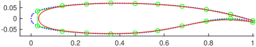
(a) Step 0, initial fitting.

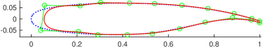
(b) Step 7.

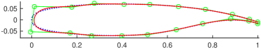
(c) Step 14.

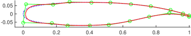
(d) Step 57, fitting result.

Figure 1: An airfoil-shape data set of 205 data points is fitted by a cubic B-spline curve with 20 control points.

For Example 2, the cubic B-spline curves generated by the MLSPIA method with the second kind of initial points at the initial step, $5$th and $10$th steps, and $64$th step are shown in Figure 2.

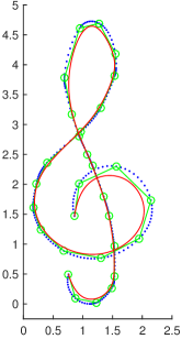
(a) Initial fitting.

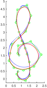
(b) Step 5.

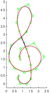
(c) Step 10.

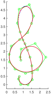
(d) Fitting result.

Figure 2: A point set of 305 points is fitted by a cubic B-spline curve with 30 control points.

For Example 3, the cubic B-spline curves generated by the MLSPIA method with the second kind of initial points at the initial step, $5$th and $10$th steps, and $47$th step are shown in Figure 3.

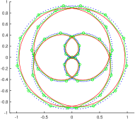
(a) Initial fitting.

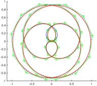
(b) Step 5.

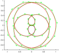
(c) Step 10.

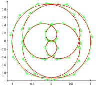
(d) Fitting result.

​​​​ ​​​​ ​​​​

Figure 3: A point set of 501 points is fitted by a cubic B-spline curve with 50 control points.

For Example $4$, the cubic B-spline curves generated by the MLSPIA method with the second kind of initial points at the initial step, $20$th and $40$th steps, and $63$th step are shown in Figure 4.

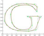
(a) Initial fitting.

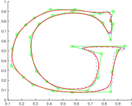
(b) Step 20.

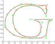
(c) Step 40.

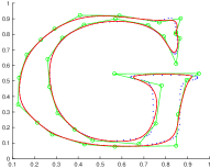
(d) Fitting result.

​​​​​​​​​ ​​​​​​​​ ​​​​​​​​

Figure 4: A point set of 269 points is fitted by a cubic B-spline curve with 35 control points.

For Example 5, the cubic B-spline tensor product surfaces generated by the MLSPIA method with the second kind of initial points at the initial step, $200$th and $362$th steps, and the original surface are shown in Figure 5.

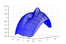
(a) Initial surface.

(b) Step 1000.

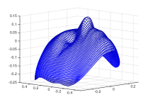
(c) Fitting result.

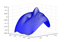
(d) Original surface.

​​​​​​​​​​​​​​​ ​​​​​​​​​​​​​​​​ ​​​​​​​​​​​​​​​​

Figure 5: A point set of $81\times 81$ points is fitted by a cubic B-spline tensor product surface with $35\times 35$ control points..

It can be seen that the fittings at the left side in Figure 1 and around the corner at the right part in Figure 4 are not very well. It is the same as what is stated in [7] for the LSPIA method. To improve the fitting result, as is described in Remark 3, it is suggested that effective techniques, such as the incremental data fitting and the shape preserving ones that are stated in [7], should be used in practice.

In Table 2, columns “IT” (iteration steps), “CPU time” (the average of CPU times in ten times) and “Weights” (the weights used in numerical experiments) for the LSPIA and MLSPIA methods are listed. The value listed in the column “MaxDeviations” for each example is defined by

$$\max_{0\leq t\leq 1}\|C_{LS}(t)-C_{MLS}(t)\|,$$

Table 2: Comparison of iteration steps, CPU times and maximum deviations at chosen weights

Examples	Methods	IT	CPU time(s)	Weights	MaxDeviations
1	MLSPIA	57	0.00094	$\omega^{\ast}=\gamma^{\ast}=0.564044574432$	$5.7533\times 10^{-11}$
				$\nu^{\ast}=0.410174207181$
	LSPIA	224	0.0030	$\mu^{\ast}=0.161116795141$
2	MLSPIA	64	0.0043	$\omega^{\ast}=\gamma^{\ast}=0.540473573417$	$8.0937\times 10^{-10}$
				$\nu^{\ast}=0.441899756336$
	LSPIA	268	0.0188	$\mu^{\ast}=0.163638791357$
3	MLSPIA	47	0.0045	$\omega^{\ast}=\gamma^{\ast}=0.589932226424$	$1.1266\times 10^{-9}$
				$\nu^{\ast}=0.418520492365$
	LSPIA	156	0.0109	$\mu^{\ast}=0.175097063057$
4	MLSPIA	63	0.0058	$\omega^{\ast}=\gamma^{\ast}=0.524388806864$	$2.5985\times 10^{-10}$
				$\nu^{\ast}=0.572453504530$
	LSPIA	272	0.0124	$\mu^{\ast}=0.203433134434$
5	MLSPIA	362	5.4167	$\omega^{\ast}=\gamma^{\ast}=0.132873535878$	$1.8688\times 10^{-10}$
				$\nu^{\ast}=4.404202175610$
	LSPIA	7576	130.6242	$\mu^{\ast}=0.313423823743$
“IT”: iteration steps, “CPU time”: average CPU times in ten runs, “Weights”: $\omega^{\ast},\gamma^{\ast},\nu^{\ast}$ are
defined by (27) for Examples 1–4 and by (37) for Example 5, and $\mu^{\ast}$ is defined by (18) in [7].

where $C_{LS}(t)$ and $C_{MLS}(t)$ with $0\leq t\leq 1$ are the least square fitting curves (or surfaces) obtained by the LSPIA and MLSPIA methods, separately. We can see that the MLSPIA method needs less iteration steps and spend less CPU time than the LSPIA method, and that the maximum deviations are very tiny.

Curvature combs for Examples 1-4 and zebra maps for Example 5 obtained by the LSPIA and MLSPIA methods are listed in Figure 6, where, upper and lower figures for Example 1 are the fitting results of the LSPIA and MLSPIA methods, separately, and left and right figures for Examples 2-5 in each row stands for the fitting results of the LSPIA and MLSPIA methods, separately. We can see that the differences in each example are very small, as is shown in Table 2.

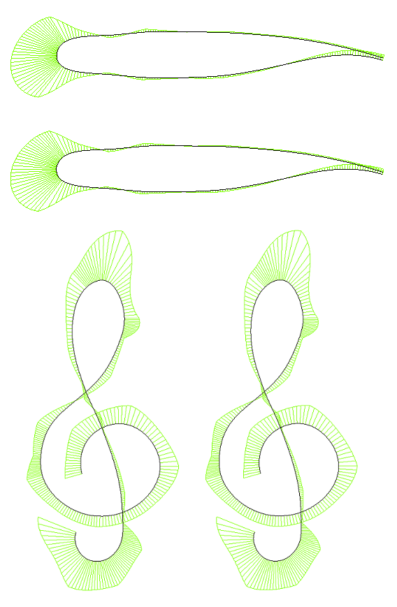
(a) Examples 1-2.

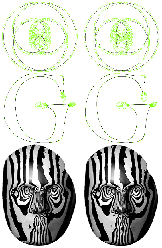
(b) Examples 3-5.

Figure 6: Curvature combs for Examples 1-4 and zebra maps for Example 5: For Example 1, upper and lower figures of are the fitting results of LSPIA and MLSPIA methods, separately. For Examples 2-5, left and right figures in each row stands for the fitting results of LSPIA and MLSPIA methods, separately.

Table 3 lists the numerical results of the MLSPIA method in ten runs based on the sparse initial control points, obtained by the rand function of Matlab, in the rectangle $[-200000,20000]^{2}$ for Examples 1-4 and in the cube $[-20000,20000]^{3}$ for Example 5. In the table, the weights are chosen as the same as that in Table 2, and columns “IT”, “CPU time” and “Errors” list the maximum and minimum numbers of iterations, CPU times in second and errors $E_{IT}$ computed via (39), separately. From the table, we can see that even for a very sparse initial control points that is far away from the given data set, the MLSPIA method will converges to the least square fitting in not too long a time.

Table 3: MLSPIA method based on random initial control points

Examples	IT	CPU time(s)	Errors $E_{IT}$	Weights
1	$86\thicksim 95$	$0.0015\thicksim 0.0028$	$6.7986\times 10^{-9}\thicksim$	$\omega^{\ast}=\gamma^{\ast}=0.564044574432$
			$9.8944\times 10^{-9}$	$\nu^{\ast}=0.410174207181$
2	$92\thicksim 100$	$0.0045\thicksim 0.0072$	$6.9669\times 10^{-9}\thicksim$	$\omega^{\ast}=\gamma^{\ast}=0.540473573417$
			$9.8188\times 10^{-9}$	$\nu^{\ast}=0.441899756336$
3	$82\thicksim 87$	$0.0056\thicksim 0.0089$	$7.1887\times 10^{-9}\thicksim$	$\omega^{\ast}=\gamma^{\ast}=0.589932226424$
			$9,6780\times 10^{-9}$	$\nu^{\ast}=0.418520492365$
4	$96\thicksim 104$	$0.0054\thicksim 0.0117$	$7.4159\times 10^{-9}\thicksim$	$\omega^{\ast}=\gamma^{\ast}=0.524388806864$
			$9.7002\times 10^{-9}$	$\nu^{\ast}=0.572453504530$
5	$533\thicksim 558$	$8.2565\thicksim 8.8496$	$9.3723\times 10^{-9}\thicksim$	$\omega^{\ast}=\gamma^{\ast}=0.132873535878$
			$9.8929\times 10^{-9}$	$\nu^{\ast}=4.404202175610$
“IT”: iteration steps, “CPU time”: CPU times, “Weights”: see Table 2, $``E_{IT}"$: computed via (39).

7 Conclusions

In this paper, a progressive and iterative approximation method with memory for least square fitting (MLSPIA) is developed. The method constructs a series of fitting curves (surfaces) with three weights by adjusting the control points and the weighted sums iteratively. It is proved that these curves (surfaces) under the suitable choices of weights will converge to the least square fitting result even when the collocation matrix is singular, and that the fastest convergence rate of the method is faster than that of the LSPIA method proposed in [7] under the same condition.

References

- Piegl L, Tiller W [1997] Piegl L, Tiller W . The NURBS book. 2nd ed.; New York, USA: Springer-Verlag; 1997.
- Farin G, Hoschek J, Kim M-S [2002] Farin G, Hoschek J, Kim M-S . Handbook of computer aided geometric design. 1st ed.; North-Holland; 2002.
- Borges CF, Pastva T [2002] Borges CF, Pastva T . Total least squares fitting of bezier and b-spline curves to ordered data. Comput-Aided Des 2002;19:275–89.
- Wang W, Pottmann H, Liu Y [2006] Wang W, Pottmann H, Liu Y . Fitting b-spline curves to point clouds by curvature-based squared distance minimization. ACM Transactions on Graphics 2006;25:214–38.
- Kineri Y, Wang M, Lin H, Maekawa T [2012] Kineri Y, Wang M, Lin H, Maekawa T . B-spline surface fitting by iterative geometric interpolation/approximation algorithms. Comput-Aided Des 2012;44(7):697–708.
- Lin H-W, Zhang Z-Y [2013] Lin H-W, Zhang Z-Y . An efficient method for fitting large data sets using T-splines. SIAM J Sci Comput 2013;35(6):A3052–68.
- Deng C-Y, Lin H-W [2014] Deng C-Y, Lin H-W . Progressive and iterative approximation for least squares B-spline curve and surface fitting. Comput-Aided Des 2014;47:32–44.
- Galveza A, Iglesiasa A, Avilaa A, Oteroc C, Ariasc R, Manchadoca C [2015] Galveza A, Iglesiasa A, Avilaa A, Oteroc C, Ariasc R, Manchadoca C . Elitist clonal selection algorithm for optimal choice of free knots in b-spline data fitting. Applied Soft Computing 2015;26:90–106.
- Zhang L, Ge X-Y, Tan J-Q [2016] Zhang L, Ge X-Y, Tan J-Q . Least square geometric iterative fitting method for generalized B-spline curves with two different kinds of weights. Vis Comput 2016;32(9):1109–20.
- Lin H, Cao Q, Zhang X [2017] Lin H, Cao Q, Zhang X . The convergence of least-squares progressive iterative approximation with singular iterative matrix. arXiv 2017;URL: arXiv:1707.09109.
- Ebrahimi A, Loghmani BG [2018] Ebrahimi A, Loghmani BG . Shape modeling based on specifying the initial b-spline curve and scaled bfgs optimization method. Multimed Tools Appl 2018;77:30331–51.
- Lin H, Maekawa T, Deng C [2018] Lin H, Maekawa T, Deng C . Survey on geometric iterative methods and their applications. Comput-Aided Des 2018;95:40–51.
- Liu M-Z, Li B-J, Guo Q-J, Zhu C-G, Hu P, Shao Y-H [2018] Liu M-Z, Li B-J, Guo Q-J, Zhu C-G, Hu P, Shao Y-H . Progressive iterative approximation for regularized least square bivariate B-spline surface fitting. J Comput Appl Math 2018;327:175–87.
- Vaitkus M, Varady T [2018] Vaitkus M, Varady T . Parameterizing and extending trimmed regions for tensor-product surface fitting. Comput-Aided Des 2018;104:125–40.
- Lin H-W, Bao H-J, Wang G-J [2005] Lin H-W, Bao H-J, Wang G-J . Totally positive bases and progressive iteration approximation. Comput Math Appl 2005;50(3-4):575–86.
- Lin H-W [2010a] Lin H-W . The convergence of the geometric interpolation algorithm. Comput-Aided Des 2010a;42(6):505–8.
- Maekawa T, Matsumoto Y, Namiki K [2007] Maekawa T, Matsumoto Y, Namiki K . Interpolation by geometric algorithm. Comput-Aided Des 2007;39(4):313–23.
- De Boor C [1979] De Boor C . How does Agee’s smoothing method work? Proceedings of the 1979 army numerical analysis and computers conference, ARO report 1979;79-3:299–302.
- Qi D, Tian Z, Zhang Y, Feng J [1975] Qi D, Tian Z, Zhang Y, Feng J . The method of numeric polish in curve fitting. Acta Mathematica Sinica 1975;18:173–84.
- Yamaguchi F [1977] Yamaguchi F . A method of designing free surfaces by computer display (1st report). Precision Machinery 1977;43(2):168–73.
- Carnicer JM, García-Esnaola M, Peña JM [1996] Carnicer JM, García-Esnaola M, Peña JM . Convexity of rational curves and total positivity. J Comput Appl Math 1996;71(2):365–82.
- Delgado J, Peña, JM [2003] Delgado J, Peña, JM . A shape preserving representation with a evaluation algorithm of linear complexity. Comput Aided Geom Design 2003;20(1):1–10.
- Lin H-W, Wang G-J, Dong C-S [2004] Lin H-W, Wang G-J, Dong C-S . Constructing iterative non-uniform B-spline curve and surface to fit data points. Sci China Ser F 2004;47(3):315–31.
- Lu L-Z [2010] Lu L-Z . Weighted progressive iteration approximation and convergence analysis. Comput Aided Geom Design 2010;27(2):129–37.
- Lin H-W, Zhang Z-Y [2011] Lin H-W, Zhang Z-Y . An extended iterative format for the progressive-iteration approximation. Comput Graph 2011;35(5):967–75.
- Shi L-M, Wang R-H [2006] Shi L-M, Wang R-H . An iterative algorithm of NURBS interpolation and approximation. J Math Res Exposition 2006;26(4):735–43.
- Lin H-W [2010b] Lin H-W . Local progressive-iterative approximation format for blending curves and patches. Comput Aided Geom Design 2010b;27(4):322–39.
- Chen J, Wang G-J [2011] Chen J, Wang G-J . Progressive iterative approximation for triangular Bézier surfaces. Comput-Aided Des 2011;43(8):889–95.
- Hu Q-Q [2013] Hu Q-Q . An iterative algorithm for polynomial approximation of rational triangular Bézier surfaces. Appl Math Comput 2013;219(17):9308–16.
- Cheng F-H, Fan F-T, Lai S-H, Huang C-L, Wang J-X, Yong J-H [2009] Cheng F-H, Fan F-T, Lai S-H, Huang C-L, Wang J-X, Yong J-H . Loop subdivision surface based progressive interpolation. J Comput Sci Tech 2009;24(1):39–46.
- Deng C-Y, Ma W-Y [2012] Deng C-Y, Ma W-Y . Weighted progressive interpolation of Loop subdivision surfaces. Comput-Aided Des 2012;44(5):424–31.
- Chen Z-X, Luo X-N, Tan L, Ye B-H, Chen J-P [2008] Chen Z-X, Luo X-N, Tan L, Ye B-H, Chen J-P . Progressive interpolation based on Catmull-Clark subdivision surfaces. Computer Graphics Forum 2008;27(7):1823–7.
- Fan F-T, Cheng F-H, Lai S-H [2008] Fan F-T, Cheng F-H, Lai S-H . Subdivision based interpolation with shape control. Computer-Aided Design and Applications 2008;5(1-4):539–47.
- De Boor C, Rice JR [1968] De Boor C, Rice JR . Least squares cubic spline approximation I-Fixed knots. Computer Sciences, Purdue University; 1968.
- Young DM [1971] Young DM . Iterative solution of large linear systems. New York-London: Academic press; 1971.
- Schöenberg IJ, Whitney A [1953] Schöenberg IJ, Whitney A . On polya frequency functions. Trans Amer Math Soc 1953;74:246–59.