: Two-stage Active Learning for Error Detection - Technical Report

Abstract.

Traditional error detection approaches require user-defined parameters and rules. Thus, the user has to know both the error detection system and the data. However, we can also formulate error detection as a semi-supervised classification problem that only requires domain expertise. The challenges for such an approach are twofold: (1) to represent the data in a way that enables a classification model to identify various kinds of data errors, and (2) to pick the most promising data values for learning. In this paper, we address these challenges with , our new example-driven error detection method. First, we present a new two-dimensional multi-classifier sampling strategy for active learning. Second, we propose novel multi-column features. The combined application of these techniques provides fast convergence of the classification task with high detection accuracy. On several real-world datasets, requires, on average, less than 1% labels to outperform existing error detection approaches.

This report extends the peer-reviewed paper ED2: A Case for Active Learning in Error Detection (neutatz2019ed2). All source code related to this project is available on GitHub.

1. Introduction

Data cleaning is an essential process in maintaining high data quality and reliable analytics. A core step in data cleaning is identifying erroneous values and repairing them.

In this paper, we consider the problem of error detection. Accurate detection of errors improves the performance of data-driven error correction methods (rekatsinas2017holoclean) and relieves data engineers from manual verification of false positives. In fact, many companies still rely on manual repair procedures (abedjan2016detecting). Research on error detection has pursued different strategies, such as rule-based (dallachiesa2013nadeef), quantitative (pit2016outlier), pattern-based (kandel2012enterprise), or dictionary-based (chu2015katara) methods. However, all these methods require either qualitative parameters, such as rules, or quantitative parameters, such as outlier thresholds. Identifying promising outlier thresholds requires the user to search and evaluate a wide range of statistical parameters. Similarly, formulating rules requires rudimentary programming knowledge, e.g., to formulate regular expressions or functional dependencies. Yet, users often are unaware of the pre-existing set of rules and have to undergo time-consuming browsing and exploration routines to identify applicable cleaning rules.

A different approach to error detection that does not require the user to have prior tool-specific knowledge or spend time wrangling with the data is to consider it as a classification task. The idea is to have the user label a subset of the dataset as erroneous or correct. Then, classification models learn to label the rest of the dataset accordingly. This approach requires only domain knowledge from the users and unburdens them from parameter tuning and rule declaration.

ActiveClean (krishnan2016activeclean) and BoostClean (krishnan2017boostclean) are two recent approaches that apply error classification for tuples. Both approaches focus on identifying and cleaning erroneous tuples based on their impact on an application-specific machine learning task, such as house price prediction. The limitation of these approaches is twofold: First, their sampling strategy for obtaining labels depends on an application-specific machine learning task. In the absence of such a task, one has to resort to a more general sampling strategy. Second, their approach and feature selection are designed to detect erroneous tuples. In many application scenarios, identifying only the tuple is not enough. One has to find the exact position of an actual data error, namely the actual data cells. To formulate a classification task for this goal, the following two challenges emerge:

Table 1. Sample dataset with errors.

Position	Salary	Phone	Company
Senior Manager	5000	1111	Stark Industries
Senior Accountant	8000	1112	PiedPiper
Junior Engineer	5000	1113	Hooli
Senior Accountant	10000	4111	Hooli
Junior Engineer	0	1114	-

Feature Representation. Errors come in various shapes and forms, such as misspellings, formatting issues, missing values, token transpositions, or semantically incorrect values. In order to generalize knowledge of labeled errors, we need features that describe the context of possible data errors.

For example, consider the motivational dataset in Table 1. Suppose the dataset contains the five errors that are marked with red background color. Certainly, one has to include features that describe how well a value fits inside a column. For example, features that identify the valid magnitude of numbers, such as ${\textit{Salary}>500}$, or features that describe the lexical appearance of values, such as Company is not empty, or phone numbers should have the prefix $11$. Additionally, one has to also featurize the relationship of each cell with all the other cells in the same row and encode co-occurrences. Consider the errors in the first tuple. In order to identify that the Salary value is wrong, the model has to learn a rule similar to ${\textit{Position}.\text{contains}(\textit{"Senior")}\rightarrow\textit{Salary}>7999}$. Finally, we might also have syntactically correct values that are still considered to be wrong according to the ground truth. For example, the company Stark Industries is from another cinematic universe and therefore an error. However, there is no apriori rule to capture this error. In this particular case, one could draw a parallel between the first and the last tuple where both the Salary and Company attributes are erroneous. So, if we can encode the classification results of the other columns as features, a classifier might be able to identify that the value in the Company column is more likely to be erroneous if the Salary had been already identified as an error.

Therefore, the first challenge is to present a general feature representation that captures a large number of error types and can be extracted automatically.

Labeling Effort. Once we have a feature set that can represent each data cell of a dataset, the next challenge is to model the classification task in a way that is efficient with regard to the required number of labels. If we employ a single classifier for the error detection task, we would have to train a multi-label classification model (tsoumakas2007multi). Because not all cells of a tuple are correct or erroneous at the same time, such a model requires a separate label for each attribute value of a tuple. Therefore, we propose to use one classifier per column, requiring a separate training set per column (tsoumakas2007multi). Each classifier can use features from the entire dataset for classifying the values of its corresponding column. We can then apply active learning, which has been shown to be effective in classification tasks with imbalanced classes (ertekin2007learning). Using one classifier per column additionally provides us with an opportunity to share insights on classification results across classifiers. This way, the models can detect error correlations across columns faster. However, considering that errors in different columns are differently hard to detect, we would need a different amount of labels for each column. This problem becomes more critical as the ratio of erroneous values to correct values in a dataset is typically imbalanced, i.e., the class of erroneous values is much smaller than the class of correct values, leading to higher diffusion of data errors inside a dataset. Therefore, we need an approach that judiciously selects the most promising columns from the dataset for labeling.

To address the aforementioned challenges, we propose the cell-wise error detection system that classifies data errors with the help of the user, who progressively labels dataset cells as erroneous or correct. In particular, we make the following contributions:

• To reduce the user labeling effort, we present a new two-dimensional multi-classifier active learning policy (Section 3) to progressively choose the appropriate cells for labeling. This active learning strategy advances standard active learning by not only finding the right cells within one column (one dimensional) but also across all columns (two dimensional).

• To cover the wide range of error types, our new example-driven error detection approach leverages a holistic set of features (Section 4) based on metadata, a character-level language model, value correlations, and error correlations. Furthermore, we leverage column-wise feature concatenation to exploit inter-column feature relationships.

• We conduct extensive experiments (Section 5) showing that our method surpasses state-of-the-art accuracy while keeping the user effort low. Furthermore, we report how different feature sets, classification models, and labeling strategies influence the performance of our method.

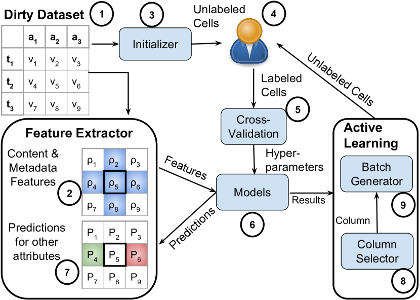
Figure 1. The workflow.

2. Problem Statement

We address the problem of error detection in relational datasets. We denote $D=\{t_{1},t_{2},...,t_{N}\}$ as a dataset of size $N$, where each $t_{i}$ represents a tuple. Let $A=\{a_{1},a_{2},...,a_{M}\}$ be the schema with attributes $a_{j}$. Then, ${D[i,j]}$ represents the cell value of the attribute $a_{j}$ in the tuple $t_{i}$. We denote $D_{C}$ as the cleaned version of $D$ representing the ground truth.

Definition 2.0.

Similar to existing literature (rekatsinas2017holoclean; abedjan2016detecting), we define an error as any cell value ${D[i,j]}$ that deviates from its ground truth value ${D_{C}[i,j]}$.

The goal of our method is to detect errors in a relational dataset $D$ by letting the user progressively label attribute values as erroneous or correct. Therefore, the first problem is to identify the right numerical feature representation $\rho$, which effectively describes the content of each cell ${D[i,j]}$. The second problem is to develop a sampling strategy that chooses the most promising training set to maximizes the error detection effectiveness, i.e., $F_{1}$-score.

The $F_{1}$-score is defined as $F_{1}=2\times(P\times R)/(P+R)$, where the precision (P) is the fraction of cells that are correctly detected as errors and the recall (R) is the fraction of the actual errors that are discovered.

3. Two-Dimensional Active Learning

Before discussing our active learning strategy, we present the overall workflow of in Figure 1. takes a dirty dataset $D$ as input ❶. The Feature Extractor generates features $\rho$ for each data cell of the dataset ❷ as described in Section 4. Then, the user receives an initial sample of cells from all columns, which should be labeled as erroneous or correct ❸. Leveraging the user-provided labels ❹, trains one classifier for each column. leverages the user-provided labels to automatically optimize the hyperparameters of the classification models using grid search and cross-validation ❺.

Afterward, applies this model to all data cells of the corresponding column and estimates the probability of a cell to be erroneous ❻. In step ❼, leverages these predictions $P$ to augment the feature vector and enables knowledge sharing across models, as we discuss in Section 4.2.3. Once the models for all columns are initialized ❻, the actual active learning process starts.

Our two-dimensional active learning policy is implemented via the Column Selector component and the Batch Generator component. As we train one classifier per column, the Column Selector has to choose the column that should be labeled next ❽. In Section 3.1, we describe how the Column Selector leverages the results of the models to make this decision. Then, the Batch Generator selects the most promising cells for the given column ❾ as detailed in Section 3.2. For each data cell in the batch, its corresponding tuple is presented to the user for manual verification ❹. After the batch of cells is labeled, the new labels are added to the training set of the corresponding column, model hyperparameters are optimized ❺, and the classifier is retrained on the new data ❻. From this point on, the process continues and repeats the steps from ❹ to ❾ in a loop.

During the entire active learning process, provides the user with a summary of the current and previous cross-validation performances, the certainty distributions, and the most decisive features per column. The active learning loop continues as long as the user is willing to provide additional labels. Then, the system applies the latest classification models for each column, marks the errors, and returns the result to the user.

Next, we explain the design of our two-dimensional active learning strategy.

3.1. Column Selection

As we train one classifier per column, we need a strategy for the Column Selector to decide the next column for user labeling. A naive approach for column selection is the random column selection strategy (RA). This strategy randomly chooses one column and lets the user label one batch of cells for this selected column. A more orderly approach is the selection in a round-robin fashion (RR). So, we assign the batches to the user for all columns in equal portions and in a circular order.

Both of the presented naive strategies do not consider that, for some columns, the model might detect errors easily and converge quickly, whereas for other columns, there might be more complex, diverse errors that cause the model to converge slower. Slower convergence also means that the user needs to label more cells to achieve the same performance. Figure 2 illustrates one example of significant differences between the convergence behavior of two columns. In this example, the optimal column selection strategy would choose to label the column City only for two iterations because after that the classifier is already relatively accurate in classifying the City values. Then, the strategy would continue to ask the user for labels for the column Middle Name. Picking the best column not only accelerates the convergence of the classifiers but also increases the quality of some of our error correlation features as described in Section 4.

Figure 2. Example of different model convergence behavior.

We studied three strategies to choose the next best column.

Min Certainty (MC). The classification model returns a probability score for each prediction, i.e., the certainty. High certainty correlates with model convergence (zhu2007active). Thus, we calculate the average certainty for all cells in a column and choose the column with the lowest average certainty.

Max Error (ME). In each iteration, we apply cross-validation on the current labeled training set for the corresponding column. The cross-validation scores are an estimate of the overall performance on the whole column data and thereby also correlate with convergence (zhu2007active). We calculate the average of all cross-validation $F_{1}$-scores per column and choose the column with the minimum average cross-validation $F_{1}$-score.

Max Prediction Change (MPC). Prediction change is the fraction of predictions that changed compared to the previous iteration. Prediction change negatively correlates with active learning convergence (bloodgood2009method). We choose the column with the highest number of prediction changes.

These column selection strategies take the convergence of the models into account to optimize the global $F_{1}$-score for the corresponding dataset. To gather all these metrics, we apply one round of round-robin first. Then, we can use one of these metrics to identify the next best column.

For the Column Selector, we choose Min Certainty because it is most stable against local optima as reported in Section LABEL:subsec:orderstrategy. For instance, if we use the Max Error strategy, we might achieve 100% $F_{1}$-score on the labeled training set, but still perform poorly on the overall dataset. Also, in the case of the Max Prediction Change strategy, a minor or no prediction change does not necessarily indicate that there is no learning progress.

3.2. Distinct Batch Sampling

Once the next column has been selected by the Column Selector component, the next step is to select actual values within a column. For the data cell values within a column, we apply standard active learning techniques. In particular, we apply the query-by-committee algorithm (settles2010active) because it is a good fit for XGBoost (chen2016xgboost) that has the fastest convergence in comparison to other models, as experiments showed in Section LABEL:sec:model_selection. Furthermore, we apply batch active learning (settles2010active) to reduce the runtime. In order to keep the sampled batch diverse, we choose cells with distinct values if possible.

3.3. Initialization

In order to be able to train a classifier, we need positive and negative examples for erroneous cells. As a minimum, we should start active learning with two erroneous and two correct cells per column. Instead of browsing through the whole dataset and identifying these cells to start up classification, we run an outlier detection method to pre-filter the possible cells. As a parameter-free variant, we employ a frequency-based ranker that ranks the values of each column by their frequency. Hence, the initial set of cells contain rare and frequent values as potential erroneous and clean training examples.

4. Feature Representation

The correct feature representation $\rho$ is critical to identify both syntactic and semantic errors. Syntactic data errors are all values that are not in the valid domain or format of the corresponding column. For example, "Londonnn" is not in the value domain of City. All errors that do not violate the syntax are called semantic errors. London as the capital of United States is a semantic error, because the value London is syntactically correct as a capital city but wrong in the given relationship.

In order to detect both syntactic and semantic errors, we have to model the context of both the patterns inside the specific column and the relationships among multiple columns. Our feature representation is a combination of existing well-known metadata features, fine-granular text features, and novel multi-column features. Before we describe the novel multi-column features, we review the set of single-column features that have been used in prior work.

4.1. Single-Column Features

We discuss two approaches to featurize a single column. First, we present a text feature representation that can be used to detect syntactic errors. Then, we discuss well-known metadata features (visengeriyeva2018metadata; pit2016outlier; krishnan2017boostclean; SchelterLSCBG18) that provide additional information to extend the text feature representation.

4.1.1. Text Features

A common way to represent text is the bag-of-words representation (harris1954distributional; krishnan2016activeclean). Relational data does not only consist of words, but also of numbers, dates, and many more diverse types of data. Furthermore, some data errors can only be discovered at a finer granularity. For instance, the salary value "1200$" requires the dollar sign to be syntactically correct. Thus, the value "1200" would be erroneous because it does not contain a dollar sign and violates the required syntax. A word-level representation would only learn this error for "1200" and would not be able to generalize it to other salary values. Using a character-level representation, the model will learn that the absence of the character ’$’ correlates with erroneous syntax. Thus, another salary value "2000" would be classified as erroneous because the value also does not contain a dollar sign. Therefore, instead of a word-level language model as used in prior work (krishnan2016activeclean), we use the more fine-granular character-level language model $\rho_{\text{n-grams}}$.

The bag-of-n-grams model is a character-based n-gram language model (cavnar1994n). Here, the Feature Extractor counts all character sequences of length $n$ occurring in a given column of the dataset. In the case of a unigram model ($n=1$), the Feature Extractor counts the occurrences of single characters, such as ’A’, ’a’, ’1’, ’.’, and ’ ’, for each cell ${D[i,j]}$ of a given column ${D[:,j]}$. The Feature Extractor applies the common approach of the TF-IDF score to normalize the n-gram counts (sparck1972statistical). Formally, we define the bag-of-n-grams feature vector as

(1)

where $\Omega_{n}(D[:,j])$ is the set of all n-grams $\omega$ of length $n$ that exist in column ${D[:,j]}$. The term frequency $\operatorname{tf}$ measures the number of times that a specific n-gram $\omega$ occurs in the cell ${D[i,j]}$ and the inverse document frequency $\operatorname{idf}$ measures whether a specific n-gram $\omega$ is common or rare across all cells in the column ${D[:,j]}$.

4.1.2. Metadata Features

Metadata can be used to complement the text features with domain-independent features that can be used to describe errors. Previous studies have shown the applicability of various metadata and statistics for data quality assessment (SchelterLSCBG18).

We leverage previously proposed metadata features: the value occurrence count $\rho_{\text{occurrence}}$ (visengeriyeva2018metadata), the string length of a value $\rho_{\text{string\_length}}$ (pit2016outlier), the data type of a value $\rho_{\text{data type}}$ (visengeriyeva2018metadata), and the numeric representation of a value $\rho_{\text{number}}$ (krishnan2017boostclean). We combine these features in a metadata feature vector of a data cell as follows:

(2) $$\begin{split}\rho_{\text{meta}}(D[i,j])=\Big{[}\rho_{\text{occurrence}}(D[i,j]),\rho_{\text{string\_length}}(D[i,j]),\\ \rho_{\text{data type}}(D[i,j]),\rho_{\text{number}}(D[i,j])\Big{]}.\end{split}$$

4.2. Feature Aggregation and Multi-Column Features

Correlations and value relationships across columns can support the error detection process. Since we have to train one classifier per column, there are several challenges and opportunities to capture inter-column relationships. We introduce three approaches to embed signals from other columns as features for a column classifier at hand. First, we adopt word embedding techniques to encode the semantic relationship of dataset values across columns. Second, we use a concatenation approach to model the relationship of labeled data cells in one column with individual features of other columns. Third, leverages prediction results of other classifiers to obtain error correlations within a tuple.

Position	Salary
senior manager	5,000
senior manager	10,000
senior manager	10,000

Figure 3. An example to show how the cell value embedding can help to detect semantic errors leveraging cell value correlations.

4.2.1. Cell Value Correlation Features

Word embeddings are a novel technique for identifying the semantic similarity of values (mikolov2013distributed). One can apply the same technique to identify correlations among values inside a dataset. To model all cell value correlations of the whole dataset, we use the Word2vec (mikolov2013distributed) features. We consider each tuple as a "document" and each cell value ${D[i,j]}$ as a "word" (krishnan2017boostclean). Then, we learn a word embedding $\rho_{\text{w2v}}$ that maps each cell value ${D[i,j]}$ into a multidimensional space $\rho_{\text{w2v}}(D[i,j])$ where co-occurring cell values are close to each other.

As shown in Figure 3, the classifier could consider all Salary values within the vicinity of the embedding of the Position value as correct, i.e., "10,000" is a correct Salary for "senior manager".

Position	Salary
senior accountant	5,000
senior manager	10,000
junior engineer	4,000
senior engineer	11,000

Figure 4. Column-wise feature concatenation: All salary values in this example have been labeled. Thus, we can use the relationship to the single-column features in Position.

4.2.2. Column-Wise Feature Concatenation

While word embeddings can be used to identify correlations at the cell value level, they do not capture correlations among more fine-granular features. For example, they cannot represent a correlation between a character "," in column A and the value string length of column B. The dataset in Figure 4 contains only distinct value pairs of Salary and Position. Therefore, there is no cell value co-occurrence. In order to learn that the salary of "senior" positions is significantly higher than that of "junior" positions, the classification model has to have access to information that concerns both Salary and Position. By concatenating the single-column features of all columns, we enable the classifier to model these fine-granular inter-column relationships.

In Figure 4, we show a decision tree that was trained based on the concatenated features of both columns Salary and Position. This model successfully identified the rule that if the Position value contains an "s" for "senior" and the Salary value is smaller than "10,000" then the Salary value is erroneous. Since we do not know upfront which inter-column relationships exist in the corresponding dataset, we concatenate features from all columns and let the classifier decide which of the features are useful.

Formally, we concatenate the single-column features of all $M$ columns as follows:

(3) $$\rho_{\text{concat}}(D[i,j],\rho)=\Big{[}\rho(D[i,1]),\dots,\rho(D[i,M])\Big{]}.$$

4.2.3. Error Correlation Features

Misfortune seldom comes alone — the same often applies to errors. Once, a classifier detects an error in one of the attributes of a tuple, it is more likely that there is an error in another attribute of the same tuple as well. In particular, there is error co-occurrence when certain tuples come from an unreliable source. For instance, in Table 1, we illustrate a potential error correlation. Whenever the Salary value is erroneous, the Company value is erroneous as well.

So far, each classification model can access only the labels of its corresponding column $j$ and therefore does not know about errors in the other columns $k$. We want to incorporate knowledge about errors in other columns. Let $\phi_{k}$ be the last trained model on the data column $k$. Further, let $P_{\phi_{k}}(D[i,k]=erroneous)$ be the estimated error probability of the data cell ${D[i,k]}$ based on the model $\phi_{k}$. Therefore, for our current column $j$, we concatenate the estimated error probabilities of all other columns $k\neq j$. Formally,

(4) $$\begin{split}\rho_{\text{error}}(D[i,j])=\Big{[}P_{\phi_{1}}(D[i,1]=\text{erroneous}),\dots,P_{\phi_{j-1}}(D[i,j-1]=\text{erroneous}),\\ P_{\phi_{j+1}}(D[i,j+1]=\text{erroneous}),\dots,P_{\phi_{M}}(D[i,M]=\text{erroneous})\Big{]}.\end{split}$$

In case of very small error fractions, it is harder to find examples for erroneous values. Our experiments show that particularly in such cases, the error correlation features improve the prediction quality of the classifiers. We add these features to the feature matrix in step ❼ of Figure 1.

4.3. Feature Vector at a Glance

The Feature Extractor concatenates all the features that can be obtained per column, i.e., the n-gram features, metadata features, Word2vec features, together with the error correlation features that are extracted after a prediction step. Formally, we can define the final feature vector per data cell ${D[i,j]}$ as follows:

(5) $$\begin{split}\rho_{\text{\system{}}}(D[i,j])=\bigg{[}\rho_{\text{concat}}(D[i,j],\rho_{\text{n-grams}}),\rho_{\text{concat}}(D[i,j],\rho_{\text{meta}}),\\ \rho_{\text{concat}}(D[i,j],\rho_{\text{w2v}}),\rho_{\text{error}}(D[i,j])\bigg{]}.\end{split}$$

4.4. Explainability

One of the reasons that data practitioners still resort to rule-based approaches is that rules are explainable. In order to explain classification results, we train simple interpretable models, such as a decision tree. By training this model on our fine-granular features, is able to provide the decision path as explanation to the user. For instance, the explanation for the erroneous value Stark Industries in Table 1 would be the following decision path: IF ${P(\text{Salary("5000")}=\text{erroneous})>0.8}$ THEN Stark Industries is erroneous. If the user detects a mistake of the classification model, the user can also prevent the model from using specific features to improve and accelerate model learning.

5. Experiments

5

Figure 5. $F_{1}$-score and labeling effort of different error detection methods for different datasets.

Table 2. Best $F_{1}$-score results of each method in Figure 5 and their corresponding precision (P) and recall (R).

1.3 Flights Movies Beers Address P R $\text{F}_{1}$ P R $\text{F}_{1}$ P R $\text{F}_{1}$ P R $\text{F}_{1}$ 0.84 $\pm$ 0.03 0.90 $\pm$ 0.02 0.87 $\pm$ 0.01 0.89 $\pm$ 0.16 0.67 $\pm$ 0.13 0.75 $\pm$ 0.12 1.00 $\pm$ 0.00 1.00 $\pm$ 0.00 1.00 $\pm$ 0.00 0.99 $\pm$ 0.01 0.96 $\pm$ 0.01 0.97 $\pm$ 0.01 ActiveClean 0.61 $\pm$ 0.03 0.50 $\pm$ 0.10 0.54 $\pm$ 0.06 0.73 $\pm$ 0.11 0.51 $\pm$ 0.07 0.60 $\pm$ 0.08 0.43 $\pm$ 0.08 0.07 $\pm$ 0.03 0.12 $\pm$ 0.04 0.49 $\pm$ 0.05 0.42 $\pm$ 0.07 0.44 $\pm$ 0.02 BoostClean 0.83 $\pm$ 0.02 0.85 $\pm$ 0.03 0.84 $\pm$ 0.02 0.60 $\pm$ 0.16 0.42 $\pm$ 0.10 0.47 $\pm$ 0.06 0.99 $\pm$ 0.04 0.54 $\pm$ 0.03 0.70 $\pm$ 0.02 0.67 $\pm$ 0.06 0.40 $\pm$ 0.07 0.50 $\pm$ 0.06 MDED 0.81 $\pm$ 0.10 0.77 $\pm$ 0.14 0.77 $\pm$ 0.04 0.68 $\pm$ 0.44 0.53 $\pm$ 0.14 0.43 $\pm$ 0.26 1.00 $\pm$ 0.00 1.00$\pm$ 0.00 1.00 $\pm$ 0.00 1.00 $\pm$ 0.00 0.82 $\pm$ 0.00 0.90 $\pm$ 0.00 dBoost 0.52 $\pm$ 0.00 1.00 $\pm$ 0.00 0.68 $\pm$ 0.00 0.24 $\pm$ 0.00 0.63 $\pm$ 0.00 0.34 $\pm$ 0.00 0.40 $\pm$ 0.00 1.00 $\pm$ 0.00 0.57 $\pm$ 0.00 0.43 $\pm$ 0.00 0.49 $\pm$ 0.00 0.45 $\pm$ 0.00 KATARA 0.09 $\pm$ 0.00 0.09 $\pm$ 0.00 0.09 $\pm$ 0.00 0.02 $\pm$ 0.00 0.16 $\pm$ 0.00 0.03 $\pm$ 0.00 0.13 $\pm$ 0.00 0.58 $\pm$ 0.00 0.21 $\pm$ 0.00 0.18 $\pm$ 0.00 0.53 $\pm$ 0.00 0.26 $\pm$ 0.00 NADEEF 0.79 $\pm$ 0.00 0.69 $\pm$ 0.00 0.74 $\pm$ 0.00 1.00 $\pm$ 0.00 0.43 $\pm$ 0.00 0.60 $\pm$ 0.00 1.00 $\pm$ 0.00 1.00 $\pm$ 0.00 1.00 $\pm$ 0.00 1.00 $\pm$ 0.00 0.83 $\pm$ 0.00 0.90 $\pm$ 0.00

We conducted several experiments to compare our approach against state-of-the-art error detection methods on multiple datasets and to benchmark different aspects of our solution. In particular, we investigate how our approach compares to state-of-the-art error detection methods in terms of effectivity and user effort. Further, we explore the influence of different feature representations, column selection strategies, and classification models on the performance of . Additional experiments with additional error detection systems and datasets can be found in our peer-reviewed paper (neutatz2019ed2).

5.1. Experimental Setup

In the following, we present the datasets, competing methods, evaluation methodology, parameter configuration, and implementation details.

5.1.1. Datasets

We conducted our experiments on four real-world datasets that mostly have been used in prior work in data cleaning. Table 3 lists these datasets along with the number of rows, number of columns, and the corresponding fraction of erroneous cells divided by all cells in the dataset.

Table 3. Experimental datasets.

Dataset	Columns		Rows		Errors
Flights	6		2,376		35%
Movies	17		7,390		1%
Beers	10		2,410		8%
Address	12		94,306		14%

Flights. Flights is a real-world dataset (li2012truth; rekatsinas2017holoclean). Errors comprise mostly wrong departure/arrival times that violate inter-column dependencies and missing values. We use this dataset to examine how stable our algorithm is in the presence of a large number of errors.

Movies. Movies is a real-world collection of movies from Rotten Tomatoes and IMDB (magellandata). Errors are mostly due to formatting issues. We use this dataset to examine if can find errors in the case of a very small error fraction.

Beers. Leveraging web scraping, multiple types of beer have been collected (beers_dataset). The errors are missing values, field separation issues, and formatting issues. We use this dataset to examine the ability of in capturing web scraping originated issues.

Address. Address is an anonymized proprietary address dataset. Errors concern spelling, formatting, completeness, and field separation. We use this dataset to examine the ability of in capturing various error types in the same dataset.

5.1.2. Baselines

We evaluate against three conventional and three novel machine learning-based competing error detection approaches.

NADEEF (dallachiesa2013nadeef) is a rule violation detection system that allows users to specify multiple types of rules to detect data errors. Usage: In addition to provided constraints by the data owners, we run Metanome (papenbrock2015data) to mine functional dependencies that are added to the set of constraints if they increase the overall $F_{1}$-score. We consider any cell that participates in at least one violation to be erroneous (abedjan2016detecting).

dBoost (pit2016outlier) is a framework that provides various machine learning models to detect outliers. In contrast to traditional outlier detection methods that are built for numerical data, dBoost proposes tuple expansion to leverage rich information across data types. Usage: We report the dBoost model with the highest $F_{1}$-score after extensive hyperparameter optimization.

KATARA (chu2015katara) can be used to detect semantic pattern violations using external knowledge bases. Usage: We provide KATARA with access to DBpedia (lehmann2015dbpedia) that contains $2017$ relations, such as has_ZIP and has_Director. Thus, potentially it can find violations for the data domains that are present in DBpedia.

ActiveClean (krishnan2016activeclean) is a machine learning model training framework that allows for iterative data cleaning. It contains an adaptive error detection component based on classification. Usage: We can not use the sampling approach of ActiveClean because it requires a user-specified machine learning task. Therefore, we apply our sampling approach while using the features proposed by ActiveClean.

BoostClean (krishnan2017boostclean) is an automated data cleaning system for machine learning datasets. Usage: The same restrictions that apply to ActiveClean, apply to BoostClean as well. Therefore, we use our sampling approach while leveraging the features proposed by BoostClean.

Metadata-driven error detection (MDED) (visengeriyeva2018metadata) aggregates the results of manually configured stand-alone error detection methods and metadata to classify errors. Usage: We provide this approach with the results from the traditional methods NADEEF, KATARA, and dBoost.

Note that these methods require configuration, such as rules, hyperparameters, and external data, whereas does not.

6

Figure 6. Comparison of different feature sets for Flights, Beers, and Address.

5.1.3. Evaluation Methodology

We measure the effectiveness of the methods in detecting potential errors using precision (P), recall (R), and $F_{1}$-score ($F_{1}$). We report the labeling effort by the number of data cell labels.

5.1.4. Our Approach

Per default, we use with the feature combination of character-level unigrams, metadata, cell value correlation, and error correlation features, and the Min Certainty column selection strategy. We choose an active learning batch size of $k=10$. Preliminary experiments show that the batch size does not significantly affect performance. As the classifier, we choose XGBoost (chen2016xgboost) because of its robustness against irrelevant features (friedman2001greedy) (see Section LABEL:sec:model_selection). For the cell value embedding space, we choose $100$ dimensions as proposed by Krishnan et al. (krishnan2017boostclean). Since is not deterministic, we apply it 10 times and report the average and the standard deviation.

5.1.5. Implementation Details

All experiments were executed on a machine with 14 2.60GHz Intel Xeon E5-2690 CPUs (each two threads), 251GB RAM, and running Ubuntu 16.04.2.

5.2. Effectiveness

In all our experiments, achieves state-of-the-art error detection $F_{1}$-score with only less than 1% labels. Figure 5 illustrates the $F_{1}$-score performance of different error detection methods with respect to the number of required labels, if applicable. The number of required labels depends on the diversity of errors. The higher the error fraction and the less diverse they appear, the fewer labels are needed. Additionally, Table 2 reports the best $F_{1}$-score result of each error detection method from Figure 5 to show the corresponding precision and recall.

The main reason for the superior performance of is that it can detect a broad set of error types, such as pattern violations, outliers, and constraint violations. Traditional methods, such as NADEEF, dBoost, and NADEEF, cannot reach the performance of because they are limited to special types of errors. For instance, on the Address dataset, covers at least 96% of the true positives of each competing method. Another advantage of over conventional methods is that can effectively exploit inter-column correlations without the help of the user. The Flights dataset requires the error detection method to exploit inter-column correlations to achieve high accuracy. For instance, for a low-quality data source, the data source identifier might correlate with erroneous values in other columns. The user might not even know about these subtle correlations. However, for Movies, ’s results differ significantly across runs. The reason for this uncertainty is that the dataset Movies has a very low error fraction. Since there are very few errors, it is harder for to find these errors and learn their pattern.

Furthermore, the experiments show that both the BoostClean and the ActiveClean features are not expressive enough and therefore achieve lower recall than .

Metadata-Driven Error Detection (MDED) converges faster at the beginning than because it leverages the results of the configured tools NADEEF, KATARA, and dBoost. However, given enough labels, always outperforms MDED. Furthermore, MDED fails to reach the performance of NADEEF for Movies due to a large number of false positives returned by KATARA.

In summary, we see that, given a small set of labels, can outperform all other error detection methods while requiring a comparably short runtime. Our approach requires slightly higher runtime than BoostClean because of the more complex features but is still faster than ActiveClean. On the largest dataset needs 12 minutes of machine time for the obtained results. Furthermore, does not require any tool-specific knowledge.

7

Figure 7. Comparison of different column selection strategies.

5.3. Micro-Benchmark Results

Next, we evaluate different internal decisions that we made for our system. First, we evaluate the features that we described in Section 4. Then, we evaluate the strategies for column selection. Finally, we evaluate different classifiers as the learning model in our system.

5.3.1. Feature Representation

Figure 6 illustrates how the $F_{1}$-score evolves based on the acc