OUJ-FTC-4
OCHA-PP-358
Beyond Squeezing à la Virasoro Algebra
So Katagiri1000So.Katagiri@gmail.com, Akio Sugamoto2,3, Koichiro Yamaguchi4, Tsukasa Yumibayashi5
1Division of Arts and Sciences, The School of Graduate Studies,
The Open University of Japan, Chiba 261-8586, Japan
2Tokyo Bunkyo Study Center, The Open University of Japan (OUJ),
Tokyo 112-0012, Japan
3Ochanomizu University, 2-1-1 Ohtsuka, Bunkyo-ku, Tokyo 112-8610, Japan
4Nature and Environment, Faculty of Liberal Arts, The Open University of Japan, Chiba 261-8586, Japan
5Department of Social Information Studies, Otsuma Women’s University, 12 Sanban-cho, Chiyoda-ku, Tokyo 102-8357, Japan
Abstract
The generalization of squeezing is realized in terms of the Virasoro algebra. The higher-order squeezing can be introduced through the higher-order time-dependent potential, in which the standard squeezing operator is generalized to higher-order Virasoro operators. We give a formula that describes the number of particles generated by the higher-order squeezing when a parameter specifying the degree of squeezing is small. The formula (18) shows that the higher the order of squeezing becomes the larger the number of generated particles grows.
1 Introduction
Squeezing has received great attention in various fields such as quantum optics [1], cosmology [2] and quantum information [3].
In particular, particle generation is an important issue; in the time-dependent oscillator, the number of produced particles is increased by repeated application of squeezing.
Accordingly, it is expected that a generalization of squeezing can increase the number of the generated particles more effectively.
Braunstein and McLachlan [5] generalized the parametric amplification by producing k-photon correlation, and numerically showed the structure of phase space. There, the usual quadratic squeezing was extended to the cases with cubic, quartic or higher-order interactions. Next, the statistics of heterodyne and homodyne detection in cubic and quartic interactions were examined by Braunstein and Caves [6]. These studies have shown that the features of higher-order interactions are well reflected in the structure of the phase space. As a review, see [4].
In this paper, we investigate the generalized squeezing from the viewpoint of the Virasoro algebra.
The Virasoro algebra is an algebra used in string theory and represents symmetry including scale transformation [7] which is called the conformal symmetry. The symmetries of parallel translation and scale transformation make up as a subalgebra of the Virasoro algebra.
Squeezing is a transformation of phase space, which preserves the area of the phase space of position and momentum. By the squeezing transformation, the position is scaled up (down) and the momentum is scaled down (up) in the opposite direction. Therefore, squeezing can be considered as a kind of scale transformation combined with parallel translation to form subalgebra of Virasoro algebra. This is the standpoint from which we construct a theory in this study.
The paper is organized as follows. First, in the next section, we introduce the Virasoro algebra with conformal symmetries. Next, in section 3, we examine the usual second-order squeezing in light of time-dependent oscillators.
In section 4, we investigate the N-th order squeezing and show that this satisfies the Virasoro algebra. In section 5, we discuss the particle generation of the N-th order squeezing. In section 6, we discuss the uncertainty relation of the N-th order squeezing. We examine the structure of the phase space of N-th order squeezing in section 7. The final section is devoted to discussion.
2 Virasoro algebra
In this section, we introduce the Virasoro algebra and see that it contains a scale transformation. Virasoro algebra is an algebra generated by generators that satisfy the following algebraic relation,
where, is called the central charge and commutes with any
and satisfies
which is subalgebra of Virasoro Algebra.
When , this algebra reduces to
which is called Witt algebra (centerless Virasoro algebra) [8].
The generator of this algebra can be constructed by and its differential operator as follows:
Then, we can understand the specific geometrical meaning of these algebras.
generates a scale transformation,
Next,
generates a parallel transformation,
Finallly,
generates a special conformal transformation,
Now, the Virasoro algebra (or Witt algebra) contains scale transformation and parallel translation in it.
3 Squeezing and time-dependent oscillators
In this section, we introduce the usual second-order squeezing, and in particular, show that the squeezed state can be obtained from time-dependent oscillators.
As is well known, in a system that describes harmonic oscillators, squeezed states are constructed by acting on the states with the following operator,
where is a squeezing parameter, and and are a creation and annihilation operator of the harmonic oscillator. The position and momentum operator are constructed as follows from and ,
We note that the generator is rewritten into the following symmetric form using and ,
Therefore, and are scaled by as follows,
The scaling factor of and are inverse with one another because is symmetric while the commutation relation antisymmetic i.e. .
These relation reduce that the squeezed state preserves the minimum uncertainty relation,
where
The squeezing opertor can be rotated to any direction, namely,
where
The time-dependent oscillators are described by,
where
In the interaction picture, the Hamiltonian can be written as,
where . The time evolution of the state can be described as follows,
where is the time ordering operator.
If we divide the time evolution operator into the product of those in a small time lapse and write,
we can write the infinitesimal time evolution operator becomes,
where is given by . If , we obtain
where . Then, in time-dependent oscillators, the time evolution of the state can be described as the repetition of the squeezing operations.
The above description is crucial in the generalization of the squeezing phenomenon in the following sections.
4 N-th order squeezing
In this section, N-th order squeezed state is represented by the Virasoro algebra, i.e. Witt algebra, as the time dependent anharmonic oscillator.
4.1 N-th order squeezing
We can construct the Virasoro algebra from the position and momentum operators in quantum mechanics111We take = 1. Here we have tentatively asssumed the operator ordering in defining (1). The more detailed analysis may give a non-vanishing central charge, but whether the analysis restores the violation of the minimum uncertainty relation for the N-th order squeezed state or not, is not clear at this moment. (See the Discussion.),
| (1) |
satisfies
This is the centerless Virasoro algebra (Witt algebra).222Here the calculation has been performed using a position representation, . This calculation can be extended to . Thus, represents a conformal transformation in space. We note here that is a generator of the usual second-order squeezing transformation.
Similarly, the dual operator of ,
| (2) |
also satisfies the Virasoro algebra,
This shows that represents a conformal transformation in space.
If we express as a harmonic oscillator, it has the following form,
We call the state, obtained by applying the unitary operator to the vacuum, an “(Virasoro) N-th order squeezed state” and write it as follows,
| (3) |
Let us examine how and are transformed by the N-th order squeezing. First,
leads to the transformation of
| (4) | |||
where . The sum can be estimated as
| (5) |
If , this equation is reduced to the usual second-order squeezing,
Next,
leads to the transformation of
| (6) | |||
This sum can also be calculated as
| (7) |
If we take the commutative limit, that is, and commute in (7), these equations yield
| (8) |
In this limit, the phase space volume is multiplied by by N-th order squeezing.
Using the and operators rotated by angle ,
the generalization of in any direction, as in the usual second-order squeezing, is naturally defined by
| (9) |
Then, can be expanded in terms of and p as follows:
| (10) | ||||
| (11) |
where is some appropriate factor. All can be expanded as the linear combination of the , namely, the algebra generated by is a generalization of the Virasoro algebra and is called algebra [9].
4.2 Time-dependent anharmonic oscillators
The time-dependent anharmonic oscillators are given by,
In the interaction picture, the Hamiltonian reads,
In the same way as in the squeezing argument, the time evolution of the state can be written as follows,
As is similar to the squeezing case, the time evolution of the state is given by
| (12) |
where .
Then, in time-dependent oscillators, the time evolution of the state can be obtained by the successive application of the N-th squeezing operators.
5 Particle production
Here we calculate the number of particle generated by N-th order squeezing. The expected number of particles in the N-th order squeezed state is written as
| (13) |
where and are
| (14) |
Here,
| (15) |
These are a generalization of the Bogolyubov transformation.
Using these equations, we obtain
| (16) |
As a result, is given by
| (17) |
where If , reproduces the result of the usual second-order squeezing,
In the case of , if is small, we can expand in and the following equation is obtained,
| (18) |
If the potential is , namely for reads
| (19) |
where is called the complementary error function, given by
If the potential is , becomes
| (20) |
where and are Bessel functions of the first and second kind.
The number of particles produced in quantum mechanics with having the time dependent potential for is plotted in fig.1.
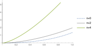
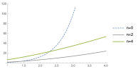
This shows that for small , the number of generated particles increase as the order of squeezing becomes higher.
6 The uncertainty relation of higher order
The usual second-order squeezed state satisfied the minimum uncertainty relation. We calculate the uncertainty relation in the case of the N-th order squeezing.
First, to determine , we note
| (21) |
is an eigenstate of because of
Then, we obtain
| (22) |
Using this vacuum state, we can calculate the uncertainty relation perturbatively in .
As a result, if is even, we obtain
| (23) |
while if is odd, we have
| (24) |
In estimating
, we will make use of
and .
As a result, if is even, we get
| (25) |
and if is odd, we have
| (26) |
From and , the uncertainty relation of N-th order squeezing is given as follows. If is even,
| (27) | ||||
If is odd,
| (28) | ||||
As an example, if we take the uncertainty relation is
| (29) |
The above results indicate that the minimum uncertainty relation is broken at the low order of perturbation in in the N-th order squeezing.
7 Phase space of the higher order
We introduce a Husimi function [10] to determine the structure of phase space. The Husimi function is defined by coherent representation,
where
For the vacuum state, , the Husimi function is
To get the N-th order squeezed Husimi function , we note
| (30) |
where we have used the following formula,
Because
the term vanishes and becomes
| (31) |
Therefore, the N-th order squeezed Husimi function is given by
| (32) |
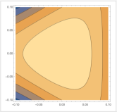
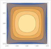
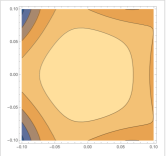
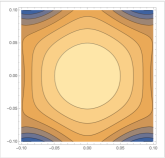
As a final result, the contour lines of phase space are depicted in fig. 2. From the figure, we have found that the N-th order squeezing is narrowed in proportion to -th square root.
8 Discussion
As the beyond squeezing effect, we have proposed the N-th order squeezing based on the Virasoro algebra, in which the N-th order squeezing is induced by the N-th order time-dependent potential. That is, the usual second-order squeezing operator is generalized to the higher-order Virasoro operators. The and are subject to local scale deformation in the opposite direction also in N-th order squeezing.
We have obtained a formula of the particle number produced by the N-th order squeezing, when the squeezing parameter is small. The formula implies that the higher the order of the squeezing is, the larger the number of generated particle is.
It is interesting to note that the extension of N-th order squeezing in any direction is related to the -algebra. The algebra of the transformation that preserves the area of phase space333This is called where is phase space of . is called -algebra, and the -algebra is its the quantized version in which the area conservation is not always preserved. These algebras represent deep connections with integrable systems [11], and the relationship between Nth-order squeezing states and integrable systems need to be further studied.
In the context of string theory, a similar Virasoro algebra and -algebra with and in the correspondence appears on the side [12]. Particles near the horizon of an extremal Reissner-Nordstrom black hole is described by conformal mechanics [13]. In , the algebra of symmetry is the Virasoro algebra, and it is possible that understanding of the relationship between the Virasoro algebra in and that in the N-th order squeezing can elucidate the role of N-th order squeezing in black holes.
In the theory of reheating after inflation, the effect of squeezing by parametric resonance has been attracting attention in connection with the problem of baryogenesis [14], and it may be applied as an effective model for the N-th order squeezing.
The N-th order squeezing obtained in this discussion can be generalized to the two-mode Bogolyubov transformation or fermionic version. It is interesting to investigate the physics, which might bring the extensions of well-known theories such as Bardeen-Cooper-Schrieffer theory [15].
These studies will be the subject in the near future.
Acknowledgments
We are deeply grateful to Shiro Komata for discussions which clarify important points on Virasoro algebra. We are indebted to Ken Yokoyama for reading this paper and giving useful comments. We would also like to thank Naoaki Fujimoto and Noriaki Aibara for reading this paper.
References
- [1] Loudon R., and Knight P. L., “Squeezed light.” J. Mod. Opt. 34.6-7 (1987): 709-759.
- [2] Kofman L., Linde A, and Starobinsky A. A., “Towards the theory of reheating after inflation.” Phys. Rev. D 56.6 (1997): 3258.
- [3] Hillery M., “Quantum cryptography with squeezed states.” Phys. Rev. A 61.2 (2000): 022309.
- [4] Dell’Anno F., De Siena S., and Illuminati F., “Multiphoton quantum optics and quantum state engineering.” Phys. Rep. 428.2-3 (2006): 53-168.
- [5] Braunstein S. L., and McLachlan R. I., “Generalized squeezing.” Phys. Rev. A 35.4 (1987): 1659.
- [6] Braunstein S. L., and Caves C. M., “Phase and homodyne statistics of generalized squeezed states.” Phys. Rev. A 42.7 (1990): 4115.
- [7] Ginsparg P., “Applied conformal field theory.” arXiv preprint hep-th/9108028 (1988).
- [8] Kac V. G., Raina A. K., and Rozhkovskaya N., “Bombay lectures on highest weight representations of infinite dimensional Lie algebras.” Vol. 29. World scientific, 2013.
- [9] Sezgin E., “Aspects of Symmetry.” arXiv preprint hep-th/9112025 (1991).
- [10] Husimi K., “Some Formal Properties of the Density Matrix” Proc.Phys. Math. Soc. Jpn. 22:264-314
- [11] Takasaki K., and Takebe T., “SDiff (2) KP hierarchy.” Int. J. Mod. Phys. A 7.supp01b (1992): 889-922.
- [12] Cacciatori S., Klemm D, and Zanon D., “w algebras, conformal mechanics and black holes.” Class. Quantum Gravity 17.8 (2000): 1731.
- [13] de Alfaro V, Fubini S., and Furlan G., “Conformal invariance in quantum mechanics.” Il Nuovo Cimento A (1965-1970) 34.4 (1976): 569-612.
- [14] Linde A., “Inflationary cosmology after Planck. ” Post-Planck Cosmology: Lecture Notes of the Les Houches Summer School: Volume 100, July 2013 100 (2015): 231.
- [15] Bardeen J., Cooper L. N., and Schrieffer J. R., “Microscopic Theory of Superconductivity”, Phys. Rev. 106, 162 - 164 (1957).