Ferromagnetism in the SU($n$) Hubbard model with a nearly flat band

Abstract

We present rigorous results for the SU($n$) Fermi-Hubbard model on the railroad-trestle lattice. We first study the model with a flat band at the bottom of the single-particle spectrum and prove that the ground states exhibit SU($n$) ferromagnetism when the total fermion number is the same as the number of unit cells. We then perturb the model by adding extra hopping terms and make the flat band dispersive. Under the same filling condition, it is proved that the ground states of the perturbed model remain SU($n$) ferromagnetic when the bottom band is nearly flat. This is the first rigorous example of the ferromagnetism in nonsingular SU($n$) Hubbard models in which both the single-particle density of states and the on-site repulsive interaction are finite.

I Introduction

Strongly correlated electron systems, in which the Coulomb interaction between electrons plays an essential role, can exhibit a variety of phenomena such as ferromagnetism, antiferromagnetism, and superconductivity. The Hubbard model has been introduced as a minimum model to describe such systems Kanamori (1963); Gutzwiller (1964); Hubbard (1963). Dispite its apparent simplicity, the intricate competition between the kinetic and the on-site Coulomb terms in the model is hard to deal with analytically. So far exact/rigorous results have been mostly limited to one dimension Essler et al. (2005) or systems with special hopping and filling Tasaki (1992); Mielke (1993); Mielke and Tasaki (1993); Tasaki (1997, shed); Derzhko et al. (2015).

Recently, it has become possible to simulate the Hubbard model using ultracold atoms in optical lattices Köhl et al. (2005); Jördens et al. (2008); Schneider et al. (2008). Furthermore, it was proposed theoretically Honerkamp and Hofstetter (2004) and demonstrated experimentally Taie et al. (2012) that multi-component fermionic systems with SU($n$) symmetry can be realized in cold-atom setups. These systems are well described by the SU($n$) Fermi-Hubbard model, in which each atom carries $n$ internal degrees of freedom. When $n=2$, the model reduces to the original Hubbard model with spin-independent interaction. Although the SU($n$) ($n>2$) symmetry has been less explored in the condensed matter literature, there is a growing interest in recent years in studying the SU($n$) Hubbard model theoretically. For example, it is argued that the SU($n$) Hubbard model can exhibit exotic phases that do not appear in the SU($2$) counterpart Cazalilla et al. (2009); Honerkamp and Hofstetter (2004); Chung and Corboz (2019). Besides, enlarged symmetry other than SU($n$), such as SO(5), in higher-spin systems has also been discussed Wu et al. (2003).

The SU($n$) Hubbard model is, in general, harder to theoretically study than the SU(2) Hubbard model. It has been reported that the Nagaoka ferromagnetism Nagaoka (1966); Tasaki (1989), which is the first rigorous result for the SU($2$) Hubbard model, can be generalized to the case of SU($n$) Katsura and Tanaka (2013); Bobrow et al. (2018). Flat-band ferromagnetism is another example of rigorous results for the SU(2) Hubbard model. Here, a flat band refers to a structure of single-particle energy spectrum which has a macroscopic degeneracy. A tight-binding model with a flat band can be constructed using standard methods such as the line-graph Mielke (1991) and the cell constructions Tasaki (1992). In the SU(2) case, it is known that if the system has a flat band at the bottom of the single-particle spectrum and the particle number is the same as the number of unit cells, the ground state of the model exhibits ferromagnetism Tasaki (1992); Mielke (1993); Tasaki (1997); Li and Shen (2004). An SU($n$) counterpart of the flat-band ferromagnetism has also been discussed recently Liu et al. (2019).

In this paper, we consider the SU($n$) Hubbard model on a one-dimensional (1D) lattice called the railroad-trestle lattice and derive rigorous results. We first treat the model with a flat band at the bottom and prove that the model exhibits SU($n$) ferromagnetism in its ground states provided that the on-site interaction is repulsive and the total fermion number is the same as the number of unit cells. This is a slight generalization of the result obtained by Liu et al. in Liu et al. (2019), in the sense that our hopping Hamiltonian has one more parameter. We then discuss SU($n$) ferromagnetism in a perturbed model obtained by adding extra hopping terms that make the flat band dispersive. We prove that this particular perturbation leaves the SU($n$) ferromagnetic ground states unchanged when the band width of the bottom band is sufficiently narrow. This is our main result and can be thought of as an SU($n$) extension of the previous theorem for the SU($2$) Hubbard model with nearly flat bands Tasaki (1995).

The rest of this paper is organized as follows. In Sec. II, we introduce the SU($n$) Hubbard model with completely flat band and prove that its ground states exhibit SU($n$) ferromagnetism. In Sec. III, we study a model with nearly flat band and prove that the ground states remain SU($n$) ferromagnetic when the repulsive interaction and the band gap are sufficiently large. We present our conclusions in Sec. IV.

II Model with completely flat band

Let $M$ be an arbitrary positive integer and $\Lambda=\{1,2,\dots,2M\}$ be a set of $2M$ sites on the railroad-trestle lattice [Fig. 1]. We impose periodic boundary condition, so that site $j$ and $j+2M$ are identified. We denote by $\mathcal{E}$ and $\mathcal{O}$ subsets of $\Lambda$ consisting of even sites and odd sites, respectively. We define creation and annihilation operators $c_{x,\alpha}^{{\dagger}}$ and $c_{x,\alpha}$ for a fermion at site $x\in\Lambda$ with color $\alpha=1,\dots,n$. They satisfy $\{c_{x,\alpha},c_{y,\beta}^{{\dagger}}\}=\delta_{\alpha,\beta}\delta_{x,y}$. The number operator of fermion at site $x$ with color $\alpha$ is denoted by $n_{x,\alpha}=c_{x,\alpha}^{{\dagger}}c_{x,\alpha}$. We consider the SU($n$) Hubbard Hamiltonian

$$H_{1} =H_{\mathrm{hop}}+H_{\mathrm{int}},$$ (1)

$$H_{\mathrm{hop}} =\sum^{n}_{\alpha=1}\sum_{x,y\in\Lambda}t_{x,y}c_{x,\alpha}^{{\dagger}}c_{y,\alpha},$$ (2)

$$H_{\mathrm{int}} =U\sum_{1\leq\alpha<\beta\leq n}\,\sum_{x\in\Lambda}n_{x,\alpha}n_{x,\beta},$$ (3)

where $t_{2x-1,2x-1}=t$, $t_{2x,2x}=2\nu^{2}t$, $t_{2x-1,2x}=t_{2x,2x-1}=\nu t$, $t_{2x-2,2x}=t_{2x,2x-2}=\nu^{2}t$, and the remaining elements of $t_{x,y}$ are zero (see Fig. 1). The parameters $t,\nu$ and $U$ are positive.

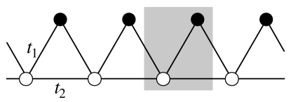
(a) (b)

Figure 1: 1 The railroad-trestle lattice with hopping amplitudes $t_{1}=\nu t$ and $t_{2}=\nu^{2}t$. Odd (black) and even (white) sites have on-site potentials $t$ and $2\nu^{2}t$, respectively. The shaded region indicates the unit cell. 1 The energy bands for $t=1,\nu=1/\sqrt{2}$. The lowest band at zero energy is completely flat.

When $U=0$, the model reduces a tight-binding model and we see that it has two bands with $\epsilon_{1}(k)=0,\epsilon_{2}(k)=t(2\nu^{2}+1)+2\nu^{2}t\cos{k}$. Clearly, the lowest band is dispersionless as shown in Fig. 1.

We define total number operators of fermion with color $\alpha$ and color-raising and lowering operators as $F^{\alpha,\beta}=\sum_{x\in\Lambda}c_{x,\alpha}^{{\dagger}}c_{x,\beta}$. Since the Hamiltonian $H_{1}$ has SU($n$) symmetry, they commute with $H_{1}$. We denote the eigenvalue of $F^{\alpha,\alpha}$ by $N_{\alpha}$. Since $F^{\alpha,\alpha}$ commute with the Hamiltonian $H_{1}$, the eigenstates of $H_{1}$ are separated into different sectors labeled by $(N_{1},\dots,N_{n})$. If the total fermion number $N_{\mathrm{f}}=\sum_{x\in\Lambda}\sum_{\alpha=1}^{n}n_{x,\alpha}$ is fixed, $N_{\alpha}$ must satisfy $\sum_{\alpha=1}^{n}N_{\alpha}=N_{\mathrm{f}}$.

Now we define a new set of operators

$$a_{x,\alpha}:=-\nu c_{x-1,\alpha}+c_{x,\alpha}-\nu c_{x+1,\alpha}\ \ \ \text{for}\ x\in\mathcal{E},$$ (4)

$$b_{x,\alpha}:=\nu c_{x-1,\alpha}+c_{x,\alpha}+\nu c_{x+1,\alpha}\ \ \ \text{for}\ x\in\mathcal{O},$$ (5)

which satisfy

$$\{a_{x,\alpha},b_{y,\beta}^{{\dagger}}\} =0,$$ (6)

$$\{a_{x,\alpha},a_{y,\beta}^{{\dagger}}\} =\begin{cases}\delta_{\alpha,\beta}(\nu^{2}+2)\ \ &\text{if}\ x=y,\\ \delta_{\alpha,\beta}\ \nu^{2}\ \ &\text{if}\ x=y\pm 2,\\ 0\ \ &\text{otherwise},\end{cases}$$ (7)

$$\{b_{x,\alpha},b_{y,\beta}^{{\dagger}}\} =\begin{cases}\delta_{\alpha,\beta}(\nu^{2}+2)\ \ &\text{if}\ x=y,\\ \delta_{\alpha,\beta}\ \nu^{2}\ \ &\text{if}\ x=y\pm 2,\\ 0\ \ &\text{otherwise}.\end{cases}$$ (8)

The hopping Hamiltonian $H_{\mathrm{hop}}$ is rewritten in terms of $b_{x,\alpha}$ and $b_{x,\alpha}^{{\dagger}}$ as

$$H_{\mathrm{hop}}=t\sum_{\alpha=1}^{n}\sum_{x\in\mathcal{O}}b_{x,\alpha}^{{\dagger}}b_{x,\alpha}$$ (9)

and hence positive semi-definite. The interaction term $H_{\mathrm{int}}$ is also positive semi-definite because $n_{x,\alpha}n_{x,\beta}=\left(c_{x,\alpha}c_{x,\beta}\right)^{{\dagger}}c_{x,\alpha}c_{x,\beta}$. Therefore, the total Hamiltonian $H_{1}=H_{\mathrm{hop}}+H_{\mathrm{int}}$ is positive semi-definite as well. From now on, we fix the total fermion number as $N_{\mathrm{f}}=|\mathcal{E}|=M$ and define a fully polarized state as $\ket{\Phi_{\mathrm{all},\alpha}}:=\prod_{x\in\mathcal{E}}a_{x,\alpha}^{{\dagger}}\ket{\Phi_{\mathrm{vac}}}$, where $\ket{\Phi_{\mathrm{vac}}}$ is a vacuum state of $c_{x,\alpha}$. From the anti-commutation relation (6), we find that $\ket{\Phi_{\mathrm{all},\alpha}}$ is an eigenstate of $H_{1}$ with eigenvalue zero. Since $H_{1}\geq 0$, the fully polarized states are ground states of $H_{1}$. Due to the SU($n$) symmetry, one obtains a general form of degenerate ground states as

$$\ket{\Phi_{N_{1},\dots,N_{n}}}=\left(F^{n,1}\right)^{N_{n}}\dots\left(F^{2,1}\right)^{N_{2}}\ket{\Phi_{\mathrm{all},1}},$$ (10)

where $N_{1}=M-\sum_{\alpha=2}^{n}N_{\alpha}$. We also refer to states of the form Eq. (10) as fully polarized states .

The first result of this paper is the following:

Theorem 1.—Consider the Hubbard Hamiltonian (1) with the total fermion number $N_{\mathrm{f}}=M$. For arbitrary $t>0$ and $U>0$, the ground states of the Hamiltonian (1) are the fully polarized states and unique apart from trivial degeneracy due to the SU($n$) symmetry.

Proof of Theorem 1.—Let $\ket{\Phi_{\mathrm{GS}}}$ be an arbitrary ground state of $H_{1}$ with $N_{\mathrm{f}}=M$. Since the ground state energy is zero, we have $H_{1}\ket{\Phi_{\mathrm{GS}}}=0$. The inequalities $H_{\mathrm{hop}}\geq 0$ and $H_{\mathrm{int}}\geq 0$ imply that $H_{\mathrm{hop}}\ket{\Phi_{\mathrm{GS}}}=0$ and $H_{\mathrm{int}}\ket{\Phi_{\mathrm{GS}}}=0$, which means that

$$b_{x,\alpha}\ket{\Phi_{\mathrm{GS}}}=0\ \ \text{for any $x\in\mathcal{O}$ and $\alpha=1,\dots n$},$$ (11)

$$c_{x,\alpha}c_{x,\beta}\ket{\Phi_{\mathrm{GS}}}=0\ \ \text{for any $x\in\Lambda$ and $\alpha\neq\beta$}.$$ (12)

Since $a_{x,\alpha}$ and $b_{x,\alpha}$ obey the anti-commutation relation (6), the condition (11) implies that $\ket{\Phi_{\mathrm{GS}}}$ does not contain any $b_{x,\alpha}^{{\dagger}}$ operator when it is constructed by acting with creation operators on the vacuum state. Therefore, it is written as

$$\ket{\Phi_{\mathrm{GS}}}$$

$$=\!\sum_{\begin{subarray}{c}A_{1},A_{2},\dots A_{n}\subset\mathcal{E}\\ \sum_{\alpha=1}^{n}|A_{\alpha}|=M\end{subarray}}\!f(\{A_{\alpha}\})\left(\prod_{x\in A_{1}}a_{x,1}^{{\dagger}}\right)\!\!\dots\!\left(\prod_{x\in A_{n}}a_{x,n}^{{\dagger}}\right)\!\!\ket{\Phi_{\mathrm{vac}}},$$ (13)

where $A_{\alpha}$ is a subset of $\mathcal{E}$ and $f(\{A_{\alpha}\})$ is a certain coefficient.

Next, we make use of the condition (12). We take an even site $x\in\mathcal{E}$. Using the anti-commutation relation $\{c_{x,\alpha},a_{y,\beta}^{{\dagger}}\}=\delta_{\alpha,\beta}\delta_{x,y}$ and Eq. (12) we see that $f(\{A_{\alpha}\})=0$ if there exist $A_{\alpha}$ and $A_{\beta}$ such that $A_{\alpha}\cap A_{\beta}\neq\emptyset$. Since $\sum_{\alpha=1}^{n}|A_{\alpha}|=M$ and $A_{\alpha}\cap A_{\beta}=\emptyset$ for $\alpha\neq\beta$, we find that $\cup_{\alpha=1}^{n}A_{\alpha}=\mathcal{E}$. This means that the ground state is rewritten as

$$\ket{\Phi_{\mathrm{GS}}}=\sum_{\bm{\alpha}}C(\bm{\alpha})\left(\prod_{x\in\mathcal{E}}a_{x,\alpha_{x}}^{{\dagger}}\right)\ket{\Phi_{\mathrm{vac}}},$$ (14)

where the sum is over all possible color configurations $\bm{\alpha}=(\alpha_{x})_{x\in\mathcal{E}}$ with $\alpha_{x}=1,\dots,n$. Then we consider the condition (12) for $x\in\mathcal{O}$. By using

$$\{c_{x,\alpha},a_{y,\beta}^{{\dagger}}\}=\begin{cases}-\nu\delta_{\alpha,\beta}\ \ &\text{if $y=x\pm 1$},\\ 0\ \ &\text{otherwise},\end{cases}$$ (15)

we get

$$c_{x,\alpha}c_{x,\beta}\ket{\Phi_{\mathrm{GS}}}$$

$$=\sum_{\begin{subarray}{c}\bm{\alpha}\\ \mathrm{s.t.}\alpha_{p}=\beta,\\ \alpha_{q}=\alpha\end{subarray}}\nu^{2}\left[C(\bm{\alpha})-C(\bm{\alpha}_{p\leftrightarrow q})\right]\left(\prod_{y\in\mathcal{E}\backslash\{x\pm 1\}}a_{y,\alpha_{y}}^{{\dagger}}\right)\ket{\Phi_{\mathrm{vac}}},$$ (16)

where $p=x-1$ and $q=x+1$. The color configuration $\bm{\alpha}_{p\leftrightarrow q}$ is obtained from $\bm{\alpha}$ by swapping $\alpha_{p}$ and $\alpha_{q}$. Since all the states in the sum are linearly independent, we find from the condition (12) that $C(\bm{\alpha})=C(\bm{\alpha}_{p\leftrightarrow q})$ for all $\bm{\alpha}$ and all $x\in\mathcal{O}$. As the two localized states on neighboring even sites share an odd site between them, we see that

$$C(\bm{\alpha})=C(\bm{\alpha}_{x\leftrightarrow y}),$$ (17)

where $x,y$ are arbitrary different sites in $\mathcal{E}$.

To show that states satisfying Eq. (17) are the fully polarized states, i.e., SU($n$) ferromagnetic, we introduce a concept of a word Kitaev (2011). A word $w=(w_{1},\dots,w_{M})$ is a sequence of integers where $w_{i}\in\{1,\dots,n\}$ for all $i$. We denote by $|w|_{\alpha}$ the number of occurences of $\alpha$ in $w$. We define the set of words for which $|w|_{\alpha}=N_{\alpha}$ holds as follows: $W(N_{1},\dots,N_{n})=\{w|\ |w|_{\alpha}=N_{\alpha},\ \alpha=1,\dots,n\}$. For example, $W(2,0,1)$ consists of $(1,1,3),(1,3,1)$ and $(3,1,1)$. It follows from Eq. (17) that the ground state of $H_{1}$ in the sector labeled by $(N_{1},\dots,N_{n})$ can be written as

$$\ket{\widetilde{\Phi}_{N_{1},\dots,N_{n}}}=\sum_{w\in W(N_{1},\dots,N_{n})}a_{2,w_{1}}^{{\dagger}}a_{4,w_{2}}^{{\dagger}}\dots a_{2M,w_{M}}^{{\dagger}}\ket{\Phi_{\mathrm{vac}}}.$$ (18)

Now using commutation relations $[F^{\beta,\alpha},a_{x,\gamma}^{{\dagger}}]=\delta_{\alpha,\gamma}a_{x,\beta}^{{\dagger}}$ for all $x\in\mathcal{E}$ , we see that

$$\left(F^{2,1}\right)^{N_{2}}\!\ket{\Phi_{\mathrm{all},1}}=\!\!\!\!\sum_{w\in W(M-N_{2},N_{2})}\!\!\!\!a_{2,w_{1}}^{{\dagger}}a_{4,w_{2}}^{{\dagger}}\dots a_{2M,w_{M}}^{{\dagger}}\ket{\Phi_{\mathrm{vac}}}.$$ (19)

By repeating the procedure, we have the desired result $\ket{\widetilde{\Phi}_{N_{1},\dots,N_{n}}}=\ket{\Phi_{N_{1},\dots,N_{n}}}$. This proves that the ground states of $H_{1}$ are fully polarized states. $\blacksquare$

III Model with nearly flat band

So far, we have considered the flat-band model, but this is an idealized case in which the lowest energy band becomes completely dispersionless. As a more realistic model, we consider a model with nearly flat band by adding a perturbation to the model in the previous section . Here we define another Hubbard model on the same lattice as Theorem 1:

$$H_{2} =H_{\mathrm{hop}}^{\prime}+H_{\mathrm{int}},$$ (20)

where $H_{\mathrm{hop}}^{\prime}$ is defined as

$$H_{\mathrm{hop}}^{\prime} =-s\sum_{\alpha=1}^{n}\sum_{x\in\mathcal{E}}a_{x,\alpha}^{{\dagger}}a_{x,\alpha}+t\sum_{\alpha=1}^{n}\sum_{x\in\mathcal{O}}b_{x,\alpha}^{{\dagger}}b_{x,\alpha},$$ (21)

and $H_{\mathrm{int}}$ is defined in Eq.(3) with parameters $s,t,U>0$. When the hopping Hamiltonian $H_{\mathrm{hop}}^{\prime}$ is written in terms of original fermion operator $c_{x,\alpha}$, it takes the form $H_{\mathrm{hop}}^{\prime}=\sum_{\alpha}\sum_{x,y\in\Lambda}t^{\prime}_{xy}c_{x,\alpha}^{{\dagger}}c_{y,\alpha}$ , where $t^{\prime}_{2x-1,2x-1}=t-2\nu^{2}s$, $t^{\prime}_{2x,2x}=-s+2\nu^{2}t$, $t^{\prime}_{2x-1,2x}=t^{\prime}_{2x,2x-1}=\nu(t+s)$, $t^{\prime}_{2x-2,2x}=t^{\prime}_{2x,2x-2}=\nu^{2}t$, $t^{\prime}_{2x-1,2x+1}=t^{\prime}_{2x+1,2x-1}=-\nu^{2}s$, and the remaining elements of $t^{\prime}_{x,y}$ are zero. When we consider the single particle problem, we obtain two bands with $\epsilon_{1}(k)=-s(2\nu^{2}+1)-2\nu^{2}s\cos{k}$, $\epsilon_{2}(k)=t(2\nu^{2}+1)+2\nu^{2}t\cos{k}$ (see Fig. 2). We see that the lowest band is no longer flat, however, it can be regarded as a nearly flat band when $s$ is small enough. We focus on this model in the following and prove a theorem on the ferromagnetism.

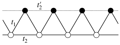
(a) (b)

Figure 2: 2 The lattice geometry of $H_{\mathrm{hop}}^{\prime}$. The hopping amplitudes are given by $t_{1}=\nu(t+s)$, $t_{2}=\nu^{2}t$, and $t_{2}^{\prime}=-\nu^{2}s$. Odd (black) and even (white) sites have on-site potentials $t-2\nu^{2}s$ and $-s+2\nu^{2}t$, respectively. The corresponding energy bands are shown in 2 for $t=1,\nu=1/\sqrt{2},s=1/10$.

Theorem 2.—Consider the Hamiltonian (20) with the total fermion number $N_{\mathrm{f}}=M$. For sufficiently large $t/s>0$ and $U/s>0$, the ground states are the fully polarized states and unique apart from the trivial degeneracy due to the SU($n$) symmetry.

Proof of Theorem 2.— First, we decompose the Hamiltonian (20) into the sum of local Hamiltonians as

$$H_{2}=-sM(2\nu^{2}+1)+\lambda H_{\mathrm{flat}}+\sum_{x\in\mathcal{E}}h_{x},$$ (22)

where

$$H_{\mathrm{flat}}=\sum_{\alpha=1}^{n}\sum_{x\in\mathcal{O}}b_{x,\alpha}^{{\dagger}}b_{x,\alpha}+\sum_{x\in\Lambda}\sum_{\alpha<\beta}n_{x,\alpha}n_{x,\beta}$$ (23)

and

$$h_{x}$$

$$=\sum_{\alpha=1}^{n}\left(-sa_{x,\alpha}^{{\dagger}}a_{x,\alpha}+\frac{t-\lambda}{2}(b_{x-1,\alpha}^{{\dagger}}b_{x-1,\alpha}+b_{x+1,\alpha}^{{\dagger}}b_{x+1,\alpha})\right)$$

$$+\frac{\kappa(U-\lambda)}{4}n_{x-2}(n_{x-2}-1)+\frac{U-\lambda}{4}n_{x-1}(n_{x-1}-1)$$

$$+\frac{(1-\kappa)(U-\lambda)}{2}n_{x}(n_{x}-1)+\frac{U-\lambda}{4}n_{x+1}(n_{x+1}-1)$$

$$+\frac{\kappa(U-\lambda)}{4}n_{x+2}(n_{x+2}-1)+s(2\nu^{2}+1),$$ (24)

where $n_{x}$ is defined as $n_{x}=\sum_{\alpha}n_{x,\alpha}$. The two parameters $\lambda$ and $\kappa$ satisfy $0<\lambda<\min\{t,U\}$ and $0\leq\kappa<1$. To prove Theorem 2, we use the following lemmas.

Lemma 1.—Suppose the local Hamiltonian $h_{x}$ is positive semi-definite for any $x\in\mathcal{E}$. Then the ground states of the Hamiltonian (22), and hence Eq. (20), are fully polarized states and unique apart from the trivial degeneracy due to the SU($n$) symmetry.

Lemma 2.—Suppose that $t,U$ are infinitely large and $0<\kappa<1$. Then the local Hamiltonian (24) is positive semi-definite. (We take $\lambda$ and $\kappa$ to be proportional to $s$.)

We note that $h_{x}$ can be regarded as a finite dimensional matrix independent of the system size since the local Hamiltonian $h_{x}$ acts nontrivially only on a finite number of sites. This means that the energy levels of $h_{x}$ depend continuously on the parameters. Therefore, Lemma 2 guarantees that $h_{x}$ is positive semi-definite when $t,U$ are finite but sufficiently large. Then Lemma 1 implies that the ground states of the Hamiltonian (20) are fully polarized states, which proves Theorem 2. $\blacksquare$

Below, we prove Lemmas 1 and 2.

Proof of Lemma 1.—First, it is noted that a fully polarized state $\ket{\Phi_{\mathrm{all},1}}=\left(\prod_{x\in\mathcal{E}}a_{x,1}^{{\dagger}}\right)\ket{\Phi_{\mathrm{vac}}}$ satisfies $h_{x}\ket{\Phi_{\mathrm{all},1}}=0$ for each $h_{x}$. Since $h_{x}$ is SU($n$) invariant, all fully polarized states have zero energy. We assume that $h_{x}\geq 0$ for all $x\in\mathcal{E}$. Let $\ket{\Phi_{\mathrm{GS}}^{\mathrm{flat}}}$ be an arbitrary ground state of $H_{\mathrm{flat}}$. Since $H_{\mathrm{flat}}\ket{\Phi_{\mathrm{GS}}^{\mathrm{flat}}}=0$ and $h_{x}\ket{\Phi_{\mathrm{GS}}^{\mathrm{flat}}}=0$, we see that $H_{2}\ket{\Phi_{\mathrm{GS}}^{\mathrm{flat}}}=-sM(2\nu^{2}+1)\ket{\Phi_{\mathrm{GS}}^{\mathrm{flat}}}$. From $h_{x}\geq 0$, the ground energy of $H_{2}$ is $-sM(2\nu^{2}+1)$. If $\ket{\Phi_{\mathrm{GS}}}$ is an arbitrary ground state of $H_{2}$, it satisfies $H_{2}\ket{\Phi_{\mathrm{GS}}}=-sM(2\nu^{2}+1)$. From $H_{\mathrm{flat}}\geq 0$ and $h_{x}\geq 0$, we find $H_{\mathrm{flat}}\ket{\Phi_{\mathrm{GS}}}=0$ and $h_{x}\ket{\Phi_{\mathrm{GS}}}=0$. This shows that any ground state of $H_{2}$ must be a ground state of $H_{\mathrm{flat}}$. The Hamiltonian $H_{\mathrm{flat}}$ is nothing but the Hamiltonian $H_{1}$ with $t=U=1$. Thus, the ground states of $H_{2}$ are fully polarized and unique. $\blacksquare$

We remark that one can check whether $h_{x}$ is positive semi-definite by numerically diagonalizing a finite dimensional matrix. The result for the SU(4) case is shown in Fig.3.

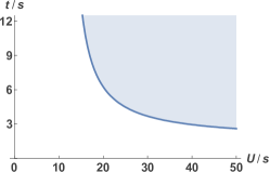
Figure 3: The positive semi-definiteness of $h_{x}$($n=4$) holds in the shaded region for $\nu=1/\sqrt{2},\kappa=0$. The plot is obtained by diagonalizing $h_{x}$ numerically. Lemma 1 says that the ground states of the full Hamiltonian $H_{2}$ are fully polarized states in the shaded region. For example, the ferromagnetism is established if $t/s\geq 4.5$ when $U/s=25$.

Proof of Lemma 2.—Due to the translational invariance, it suffices to show the case for $h_{0}$. The local Hamiltonian $h_{0}$ is regarded as an operator defined on five sites $\{-2,-1,0,1,2\}$, where $x=-2,-1$, and $0$ are identified with $x=2M-2,2M-1$, and $2M$, respectively. On these sites, we define operators

$$\tilde{a}_{-2,\alpha} :=\frac{1}{\sqrt{\nu^{2}+1}}(c_{-2,\alpha}-\nu c_{-1,\alpha}),$$ (25)

$$\tilde{b}_{-1,\alpha} :=\nu c_{-2,\alpha}+c_{-1,\alpha}+\nu c_{0,\alpha},$$ (26)

$$\tilde{a}_{0,\alpha} :=-\nu c_{-1,\alpha}+c_{0,\alpha}+-\nu c_{1,\alpha},$$ (27)

$$\tilde{b}_{1,\alpha} :=\nu c_{0,\alpha}+c_{1,\alpha}+\nu c_{2,\alpha},$$ (28)

$$\tilde{a}_{2,\alpha} :=\frac{1}{\sqrt{\nu^{2}+1}}(-\nu c_{1,\alpha}+c_{2,\alpha}).$$ (29)

These operators satisfy

$$\{\tilde{a}_{y,\alpha},\tilde{a}_{y^{\prime},\beta}^{{\dagger}}\} =\begin{cases}\delta_{\alpha,\beta}(2\nu^{2}+1)\ \ &\text{for}\ \ y=y^{\prime}=0,\\ \delta_{\alpha,\beta}\frac{\nu^{2}}{\sqrt{\nu^{2}+1}}\ \ &\text{for}\ \ |y-y^{\prime}|=2,\\ \delta_{\alpha,\beta}\delta_{y,y^{\prime}}\ \ &\text{for}\ \ y,y^{\prime}=\pm 2,\end{cases}$$ (30)

$$\{\tilde{a}_{y,\alpha},\tilde{b}_{y^{\prime},\alpha}^{{\dagger}}\} =0.$$ (31)

Single-fermion states corresponding to these operators are linearly independent. To show the lemma, we only need to consider states $\ket{\Phi}$ which have finite energy in this limit, i.e., $\lim_{t,U\rightarrow\infty}\bra{\Phi}h_{0}\ket{\Phi}<\infty$ . The condition that $\ket{\Phi}$ has finite energy is equivalent to the following:

$$\tilde{b}_{y,\alpha}\ket{\Phi} =0\ \ \text{for $y=\pm 1$},$$ (32)

$$c_{y,\alpha}c_{y,\beta}\ket{\Phi} =0\ \ \text{for $y=0,\pm 1,\pm 2$}.$$ (33)

Let $\ket{\Phi}$ be a state which has finite energy. From Eqs. (32) and (33) with $y=-2,0,2$, $\ket{\Phi}$ is written as

$$\ket{\Phi}=\!\!\!\sum_{\begin{subarray}{c}A_{1},\dots,A_{n}\subset\widetilde{\mathcal{E}}\\ A_{\alpha}\cap A_{\beta}=\emptyset\end{subarray}}\!\!f(\{A_{\alpha}\})\!\left(\prod_{y\in A_{1}}\tilde{a}_{y,1}^{{\dagger}}\right)\!\dots\!\left(\prod_{y\in A_{n}}\tilde{a}_{y,n}^{{\dagger}}\right)\!\ket{\Phi_{\mathrm{vac}}},$$ (34)

where $\widetilde{\mathcal{E}}=\{-2,0,2\}$ and $A_{\alpha}$ is an arbitrary subset of $\widetilde{\mathcal{E}}$. Since $\widetilde{\mathcal{E}}$ contains three sites, the particle number of finite energy states must be less than or equal to three. Using the condition Eq. (33) with $y=\pm 1$, we see that all the finite energy states $\ket{\Phi}$ must be a fully polarized state over the five sites and have zero energy when the particle number is three. For one-particle states, all the eigenvalues of $h_{0}$ are non negative. Thus we only need to verify the positive semi-definiteness for two-particle sectors labeled by $(N_{\alpha},N_{\beta})=(2,0)$ and $(N_{\alpha},N_{\beta})=(1,1)$. To this end, we solve the eigenvalue problem for $Ph_{0}P$ where $P$ denotes the projection operator onto the space of finite energy states. In the sector $(2,0)$, we find that there are three eigenstates

$$\ket{\Phi_{1}} =\tilde{a}_{-2,\alpha}^{{\dagger}}\tilde{a}_{0,\alpha}^{{\dagger}}\ket{\Phi_{\mathrm{vac}}},$$ (35)

$$\ket{\Phi_{2}} =\tilde{a}_{0,\alpha}^{{\dagger}}\tilde{a}_{2,\alpha}^{{\dagger}}\ket{\Phi_{\mathrm{vac}}},$$ (36)

$$\ket{\Phi_{3}}\! =\!\left[\frac{\nu^{2}}{\nu^{2}+1}(\tilde{a}_{-2,\alpha}^{{\dagger}}\!-\!\tilde{a}_{2,\alpha}^{{\dagger}})\tilde{a}_{0,\alpha}^{{\dagger}}\!-\!(2\nu^{2}+1)\tilde{a}_{-2,\alpha}^{{\dagger}}\tilde{a}_{2,\alpha}^{{\dagger}}\right]\ket{\Phi_{\mathrm{vac}}}$$ (37)

and their corresponding eigenenergies are 0, 0, and $s(2\nu^{2}+1)$, respectively. In the sector $(1,1)$, there are four eigenstates. Three of them can be obtained by applying $F^{\beta,\alpha}$ to the states $\ket{\Phi_{1}},\ket{\Phi_{2}}$ and $\ket{\Phi_{3}}$. As a state orthogonal to them, we get a singlet state

$$\ket{\Phi_{4}}=\left(\tilde{a}_{-2,\alpha}^{{\dagger}}\tilde{a}_{2,\beta}^{{\dagger}}-\tilde{a}_{-2,\beta}^{{\dagger}}\tilde{a}_{2,\alpha}^{{\dagger}}\right)\ket{\Phi_{\mathrm{vac}}},$$ (38)

and we find that this state satisfies

$$Ph_{0}P\ket{\Phi_{4}}=s(2\nu^{2}+1)\ket{\Phi_{4}}.$$ (39)

Clearly, the state $\ket{\Phi_{4}}$ has a positive energy. Hence, we see that all the eigenvalues of $h_{0}$ are nonnegative. Thus, we have proved Lemma 2. $\blacksquare$

IV Conclusion

We have presented an extension of flat-band ferromagnetism to the SU($n$) Hubbard model on the railroad-trestle lattice. Furthermore, we proved that in the nearly flat-band case, all the ground states are fully polarized if $t$ and $U$ are sufficiently large. One can similarly construct and analyze models in higher dimensions, in which the ground states are fully polarized if the lowest band is completely flat. The previous results for the SU(2) Hubbard models in higher dimensions suggest that the parameter $\nu$ has to be larger than a threshold value $\nu_{c}>0$ when the lowest band is nearly flat Shen (1998); Tasaki (2003). The details will be discussed elsewhere.

Although we have focused on models with a nonzero band gap, it would be interesting to see if the method developed in this paper can be extended to include SU($n$) Hubbard models with gapless flat or nearly flat bands Tanaka and Ueda (2003). It would also be interesting to study SU($n$) ferromagnetism in systems with topological flat bands carryng nontrivial Chern number, as its SU($2$) counterpart has been discussed in Katsura et al. (2010). Another direction for future research is to explore ferromagnetism in multiorbital Hubbard models, including the one with SU($n$) symmetry. In such systems, rigorous Li et al. (2014); Li (2015) and numerical results Xu et al. (2015) about ferromagnetism, which are different from the flat-band scenario, have been obtained recently. It is thus interesting to see to what extent our results can be generalized to the multiorbital case.