Non-spreading matter-wave packets in a ring

Abstract

Non-spreading wave packets and matter-wave packets in ring traps both have attracted great research interests due to their miraculous physical properties and tempting applications for quite a long time. Here, we proved that there exists only one set of non-spreading matter-wave packets in a free ring, and this set of wave packets have been found analytically. These non-spreading matter-wave packets can be realized in a toroidal trapped Bose-Einstein condensate system with the help of Feshbach resonance to eliminate contact interaction between atoms. Since experimentally residual interaction noise will always exist, its effect on the stability of these non-spreading wave packets is also examined. Qualitatively, under weak residual interaction noise, these non-spreading wave packets can preserve their shape for quite a long time, while a stronger interaction noise will induce shape breathing of the wave packets. Shape-keeping abilities of these wave packets are further studied quantitatively. We found that this set of wave packets have the same shape-keeping ability against interaction noise. And, the shape-keeping ability is linearly related to the interaction noise strength.

,

Keywords: Non-spreading matter-wave, Ring trap, Bose-Einstein condensate

1 Introduction

Matter-waves with substantial intensity are crucial in applications such as atom lithography [1, 2, 3], ultra-sensitive magnetometry [4, 5], matter-wave interferometry [6, 7, 8]. When a matter-wave packet propagates in free space, it will spread due to dispersion, and its intensity will decrease [9, 10]. Thus, non-spreading matter-wave packets attract great research interests. It is well known that self-focusing nonlinearity can be introduced to overcome the dispersion spreading, and form bright matter-wave solitons [11, 12, 13, 14] which are non-spreading wave packets. Soliton-based matter-wave interferometers have been elaborated in many theoretical works [15, 16, 17, 18, 19], and also experimentally implemented with an increase of interference fringe visibility been observed [20, 21]. However, nonlinearity may also do harm to the performance of interferometers, it would induce a phase diffusion, which will reduce the coherent time [22, 23]. And recently it is also reported that the best sensitivity of a matter-wave interferometer is reached in the linear regime [24, 25]. (We note that the relation between nonlinearity and performance of an interferometer is quite subtle. Besides the above-mentioned effects, nonlinearity also gives rise to non-classical correlations and squeezed states [26, 27]. Taking advantage of these properties, standard quantum limit surpassed interferometers can be realized [28, 29].) So, achieving linear non-spreading matter-wave packets can be a charming research subject.

In 1979, Berry and Balazs showed that the free particle linear Schrödinger equation has a nontrivial Airy function solution which holds its shape during an accelerating propagation [30]. After this pioneering work, such linear non-spreading waves were extensively studied (for a review see reference [31]), and first experimentally demonstrated in optical system in 2007 [32]. Soon after, linear non-spreading matter-waves were also realized in electron beams [33]. Atomic Bose-Einstein condensate (BEC), because of its macroscopic quantum properties and highly controllable feature, is an ideal system for exploring matter-wave optical phenomena. Recently, generation of similar non-spreading BEC wave packets by amplitude or phase imprinting techniques [34], and time dependent harmonic traps [35] have also been proposed.

Due to potential applications in realizing matter-wave Sagnac interferometer [36, 37, 38, 39, 40], atomic analogy of SQUID circuits [41, 42, 43], persistent current [44, 45, 46, 47] and quantum time crystal [48, 49, 50], non-spreading matter-wave packets in a ring also deserve considerable research interests. Now the point is that, we are inquisitive about whether non-spreading wave packets can exist in a free ring. In this article, first we analytically found a set of non-spreading wave packets in a free ring, at the same time we also proved that they are the only set. Then the realization of these non-spreading wave packets in atomic BEC system with the help of Feshbach resonance [51, 52] technique to eliminate inter-atom interaction is discussed. At last, although in principle inter-atom interaction can be totally eliminated by Feshbach resonance technique, practically it is impossible to operate the Feshbach magnetic field with infinite precision, and there will always exist some residual interactions [22, 23, 53], therefor the stability of these non-spreading wave packets against residual interaction noise is also studied.

The paper is organized as follows. In section 2, formulas describing non-spreading wave packets in a ring are derived, and the only set of non-spreading matter-wave packets are found analytically. In section 3, the experimental realization of the non-spreading wave packets in BEC systems are discussed briefly. In section 4, the stability of the wave packets against residual interaction noise is studied numerically. At last, the work is summarized in section 5.

2 Non-spreading matter-wave packets in a ring

To generally discuss the problem of non-spreading wave packets in a ring, we begin with the following dimensionless Schrödinger equation

$$i\frac{\partial}{\partial t}\psi\left(\theta,t\right)=-\frac{1}{2}\frac{\partial^{2}}{\partial\theta^{2}}\psi\left(\theta,t\right),$$ (1)

where $\theta$ is the azimuthal angle which takes value in range of $-\pi$ to $\pi$. Here we are interested in the case of a free ring, therefore in the equation there only exists the kinetic energy term, while external potential term is not included. The continuous of wave function and its first order derivative require

$$\psi\left(\theta_{0},t\right)=\psi\left(\theta_{0}+2n\pi,t\right),$$ (2)

and

$$\psi^{\prime}\left(\theta_{0},t\right)=\psi^{\prime}\left(\theta_{0}+2n\pi,t\right),$$ (3)

where $\theta_{0}$ is an arbitrary amizuthal angle, $n=0,\pm 1,\pm 2,\cdots$ is an integer number, and $\psi^{\prime}\left(\theta_{0},t\right)=\left.\frac{\partial\psi\left(\theta,t\right)}{\partial\theta}\right|_{\theta=\theta_{0}}$ is the first order derivative of $\psi\left(\theta,t\right)$ at point $\theta=\theta_{0}$.

To find a shape preserving wave packet, we rewrite the wave function $\psi\left(\theta,t\right)$ as follows [54, 55],

$$\psi\left(\theta,t\right)=A\left(\theta,t\right)e^{iS\left(\theta,t\right)},$$ (4)

where $A$ and $S$ are two real number functions, representing the probability density and phase distribution respectively. Under such a form, if function $A\left(\theta,t\right)$ can be expressed as $A\left(\theta,t\right)=A\left(\phi\right)$ with

$$\phi=\theta-f\left(t\right),$$ (5)

the wave packet will preserve its shape during the propagation. Here $\phi$ can be regarded as the trajectory function of the wave packet, with $f\left(t\right)$ being a real number function.

Inserting the Madelung transformed wave function (4) into Schrödinger equation (1), and splitting real and imaginary parts of the equation, we get the following two equations

$$-\frac{\partial A}{\partial\phi}\frac{df}{dt}=-\frac{1}{2}\left[2\frac{\partial A}{\partial\phi}\frac{\partial S}{\partial\theta}+A\frac{\partial^{2}S}{\partial\theta^{2}}\right],$$ (6)

and

$$-A\frac{\partial S}{\partial t}=-\frac{1}{2}\left[\frac{\partial^{2}A}{\partial\phi^{2}}-A\left(\frac{\partial S}{\partial\theta}\right)^{2}\right].$$ (7)

The first equation (6) can be rearranged into the following form

$$\frac{\partial}{\partial\theta}\left(\frac{df}{dt}A^{2}-\frac{\partial S}{\partial\theta}A^{2}\right)=0,$$

which means that $\frac{df}{dt}A^{2}-\frac{\partial S}{\partial\theta}A^{2}$ is independent of azimuthal angle $\theta$. So we can write it as

$$\left[\frac{df\left(t\right)}{dt}-\frac{\partial S\left(\theta,t\right)}{\partial\theta}\right]A^{2}\left(\phi\right)=c\left(t\right),$$ (8)

with $c\left(t\right)$ being an arbitrary function depending on time variable $t$ only.

First, it can be obviously seen that equation (8) admits a trivial solution

$$A\left(\phi\right)=cons,\quad S\left(\theta,t\right)\propto\theta.$$

Equation (7) and wave function continuous condition (2, 3) also considered, corresponding wave function reads

$$\psi\left(\theta,t\right)=Ce^{il\theta+il^{2}t/2},$$ (9)

which is a trivial solution with uniformly distributed density in the ring at all time.

If $A\left(\phi\right)$ is not a constant, by adapting its background value, there always exists an angle $\phi_{0}$ making $A\left(\phi_{0}\right)=0$. And note that the right-hand side of equation (8) is only a function of $t$, this is to say for all $\phi$ the following equation need to be satisfied

$$\left[\frac{df\left(t\right)}{dt}-\frac{\partial S\left(\theta,t\right)}{\partial\theta}\right]A^{2}\left(\phi\right)=c\left(t\right)=0.$$

From this equation, we get the following relationship between $f\left(t\right)$ and $S\left(\theta,t\right)$

$$\frac{df\left(t\right)}{dt}=\frac{\partial S\left(\theta,t\right)}{\partial\theta}=\sum_{i=0}^{\infty}c_{i}t^{i},$$ (10)

here since $\frac{df\left(t\right)}{dt}$ is a function only depending on time variable $t$, we expand it in Taylor series with $c_{j}$ being the $j$-th order coefficient. In the very following content, depending on the highest order of this series we discuss the problem in three distinct cases:

1. If series (10) only has the constant term, i.e.,

   $$\frac{df\left(t\right)}{dt}=\frac{\partial S\left(\theta,t\right)}{\partial\theta}=c_{0},$$

   then it is straightforward to get

   $$f\left(t\right)=c_{0}t,$$

   $$S\left(t\right)=c_{0}\theta+g\left(t\right),$$

   with $g\left(t\right)$ being an arbitrary function. Substituting them into equation (7), we have

   $$-A\left(\phi\right)\frac{\partial S\left(\theta,t\right)}{\partial t}=-\frac{1}{2}\left[\frac{\partial^{2}A\left(\phi\right)}{\partial\phi^{2}}-A\left(\phi\right)c_{0}^{2}\right].$$

   Because the right-hand side of this equation does not explicitly depend on time variable $t$, the equality requires $\frac{\partial S\left(\theta,t\right)}{\partial t}=\frac{dg\left(t\right)}{dt}$ is also explicitly time independent. That is to say, function $g\left(t\right)$ must take the following linear form

   $$g\left(t\right)=G_{1}t+G_{0},$$

   where $G_{0}$ and $G_{1}$ are two free constant parameters. At last, equation (7) becomes

   $$\frac{\partial^{2}A\left(\phi\right)}{\partial\phi^{2}}+\left(c_{0}^{2}-2G_{1}\right)A\left(\phi\right)=0,$$

   from which the shape of a non-spreading wave packet can be determined

   $$A\left(\phi\right)=C\cos\left(m\phi\right).$$

   Here $m=\sqrt{\left|c_{0}^{2}-2G_{1}\right|}$ is an integer number which is restricted by the boundary condition, $C$ is a normalization constant. At the same time, boundary conditions also require that $c_{0}$ be an integer number $c_{0}=l$. At last, putting the above expressions of $f,g,A,S$ all together, a full non-spreading solution can be constructed as

   $$\psi\left(\theta,t\right)= C\cos\left(m\theta-lt\right)$$ (11)

   $$\exp\left[il\theta+i\frac{\left(m^{2}+l^{2}\right)}{2}t\right].$$

   The physical meanings of $m$ and $l$ are obvious. $2m$ is number of nodes of the wave function, and $l/m$ describes the moving speed of the wave packet along the ring. We also note that the previous trivial solution (9) is just the $m=0$ specification of solution (11).

2. If series (10) has terms up to the first order, i.e.,

   $$\frac{df\left(t\right)}{dt}=\frac{\partial S\left(\theta,t\right)}{\partial\theta}=c_{0}+c_{1}t,$$

   function $f\left(t\right)$ and $S\left(\theta,t\right)$ are integrated to be

   $$f\left(t\right)=c_{0}t+\frac{1}{2}c_{1}t^{2},$$

   $$S\left(\theta,t\right)=c_{0}\theta+c_{1}\theta t+g\left(t\right).$$

   Then equation (7) becomes

   $$\frac{1}{2}\frac{\partial^{2}A\left(\phi\right)}{\partial\phi^{2}}-c_{1}\phi A\left(\phi\right)-\frac{1}{2}c_{0}^{2}A\left(\phi\right)$$

   $$= A\left(\phi\right)\left[g^{\prime}\left(t\right)+2c_{0}c_{1}t+c_{1}^{2}t^{2}\right].$$

   As in case (1), the left-hand side of this equation also does not explicitly depend on variable $t$. And in this case, equality between the left and right-hand sides can be met by the following function of $g\left(t\right)$,

   $$g\left(t\right)=-\frac{1}{3}c_{1}^{2}t^{3}+c_{0}c_{1}t^{2}+G_{1}t+G_{0}.$$

   At last, the equation governing function $A\left(\phi\right)$ reads

   $$\frac{1}{2}\frac{\partial^{2}A\left(\phi\right)}{\partial\phi^{2}}-c_{1}\phi A\left(\phi\right)-\left(\frac{1}{2}c_{0}^{2}+G_{1}\right)A\left(\phi\right)=0,$$

   which promises an Airy function solution. But an Airy function cannot fulfill the periodical boundary condition (2) and (3), therefore a non-spreading wave packet cannot exist in this situation.

3. If the series have terms equal or higher than second order, i.e.,

   $$\frac{df\left(t\right)}{dt}=\frac{\partial S\left(\theta,t\right)}{\partial\theta}=c_{0}+c_{1}t+c_{2}t^{2}+\cdots,$$

   we have

   $$f\left(t\right)=c_{0}t+\frac{1}{2}c_{1}t^{2}+\frac{1}{3}c_{2}t^{3}+\cdots,$$

   $$S\left(\theta,t\right)=\theta\left(c_{0}+c_{1}t+c_{2}t^{2}+\cdots\right)+g\left(t\right).$$

   Similar as in case (1) and (2), we rewrite equation (7) as follows

   $$\frac{1}{2}\frac{\partial^{2}A}{\partial\phi^{2}}-c_{1}\phi A-\frac{1}{2}c_{0}^{2}A=A\left[\begin{array}[]{c}\left(c_{0}c_{1}+2c_{2}\phi\right)t\\ +\left(c_{1}^{2}+2c_{0}c_{2}\right)t^{2}\\ +\cdots+g^{\prime}\left(t\right)\end{array}\right]$$

   The left-hand side of this equation is still $t$ independent. But because of the existence of new term $2c_{2}\phi t$ (and some other higher order ones), there does not exists any function $g\left(t\right)$ which can make the right-hand side also being time independent. Thus, this equation has no solution. There does not exist non-spreading wave packet solutions in such a case.

Now, in a brief summary, combing all the three above cases, we can conclude that the only set of non-spreading wave packets in a ring is given by equation (11). This set of non-spreading wave packets travel along the ring with a constant velocity. Moreover, owing to the quantum feature, these non-spreading wave packets can only propagate in some quantized fractional velocities. And unlike in free space, self-accelerating non-spreading wave packets with Airy function like form cannot exist in a ring configuration.

3 Realization in a toroidal trapped BEC system

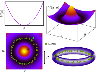
Figure 1: Diagram of toroidal trapped BEC. By applying a harmonic trap $V\left(z\right)=m\omega_{z}^{2}z^{2}/2$ along $z$-direction, a two-dimensional harmonic trap and a Gaussian barrier $V\left(x,y\right)=V\left(r,\theta\right)=m\omega^{2}r^{2}/2+V_{0}\exp\left(-2r^{2}/w_{0}^{2}\right)$ in $x$-$y$ plane, BEC can be trapped in a ring with radius $R$ determined by formula $R^{2}=w_{0}^{2}/2\ln\left[4V_{0}/\left(m\omega^{2}w_{0}^{2}\right)\right]$. If the trap along $z$ and $r$ direction is sufficiently strong, the system can be reduced to one-dimension, leaving only the space variable $\theta$ to take effect.

The non-spreading matter-wave packets found in section 2, could be experimentally realized in a quasi-one-dimensional toroidal trapped dilute atomic BEC system, see figure 1. In a BEC system, because of collision between atoms, besides the kinetic energy and external trap potential, there will also exists a nonlinear term, i.e., the system is described by the following nonlinear Schrödinger equation (Gross-Pitaevskii equation)

$$i\hbar\frac{\partial}{\partial t}\psi=-\frac{\hbar^{2}}{2m}\nabla^{2}\psi+V\left(r,\theta,z\right)\psi+g\left|\psi\right|^{2}\psi,$$ (12)

where $\hbar$ is the reduced Planck constant, $m$ is the mass of atom, $g=4\pi\hbar^{2}a_{s}/m$ is the interaction strength with $a_{s}$ being the s-wave scattering length, and

$$V\left(r,\theta,z\right)=\frac{1}{2}m\omega_{z}^{2}z^{2}+\frac{1}{2}m\omega^{2}r^{2}+V_{0}\exp\left[-\frac{2r^{2}}{w_{0}^{2}}\right],$$ (13)

is the toroidal trapping potential which is experimentally realized by a magnetic trap and a plug laser beam with Gaussian shape [46] (there are also some other schemes to realize a toroidal trap, such as the ones in ref [56, 57, 58, 59], et al.) having its minimum at $z=0$ and $r=R$, with

$$R^{2}=\frac{w_{0}^{2}}{2}\ln\left(\frac{4V_{0}}{m\omega^{2}w_{0}^{2}}\right).$$ (14)

Expanding the trapping potential around $r=R$ into Taylor series, and neglecting the third and higher orders of $r-R$, the potential approximately reads

$$V\left(r,\theta,z\right)=\frac{1}{2}m\omega_{z}^{2}z^{2}+\frac{1}{2}m\omega_{r}^{2}\left(r-R\right)^{2},$$ (15)

with $\omega_{r}=2\omega R/w_{0}$ being the effective radial trapping frequency.

For sufficiently strong confinement in axial and radial direction, the wave function can be assumed to have variables separated form $\psi=\rho_{0}\left(r\right)\phi_{0}\left(z\right)\psi\left(\theta,t\right)$ with $\phi_{0}=\left[m\omega_{z}/\left(\pi\hbar\right)\right]^{1/4}\exp\left[-\frac{m\omega_{z}z^{2}}{2\hbar}\right]$, $\rho_{0}=\left[m\omega_{r}/\left(\pi\hbar r^{2}\right)\right]^{1/4}\exp\left[-\frac{m\omega_{r}\left(r-R\right)^{2}}{2\hbar}\right]$ being ground state wave function of the axial and radial traps. Inserting it into equation (12), the system can be reduced to one-dimension. The azimuthal wave function $\psi\left(\theta,t\right)$ obeys equation

$$i\hbar\frac{\partial}{\partial t}\psi=-\frac{\hbar^{2}}{2mR^{2}}\frac{\partial^{2}}{\partial\theta^{2}}\psi+\tilde{g}\left|\psi\right|^{2}\psi.$$ (16)

Here $\tilde{g}=m\sqrt{\omega_{z}\omega_{r}}g/\left(2\pi\hbar R\right)$ is the quasi-one-dimensional effective contact interaction strength. Taking transformation $t\rightarrow mR^{2}t/\hbar$, equation (16) can be rescaled to the following dimensionless form

$$i\frac{\partial}{\partial t}\psi=-\frac{1}{2}\frac{\partial^{2}}{\partial\theta^{2}}\psi+g_{s}\left|\psi\right|^{2}\psi,$$ (17)

with $g_{s}=\tilde{g}mR^{2}/\hbar^{2}=2mRNa_{s}\sqrt{\omega_{r}\omega_{z}}/\hbar$. Considering, for instance, BEC of ${}^{39}K$ atoms, with atoms number $N=10^{3}$, s-wave scattering length $a_{s}=33a_{0}$ ($a_{0}$ is Bohr radius), trapped in a toroidal trap with parameters $R=10\mu m,\omega_{r}=\omega_{z}=1000Hz$, the interaction strength is $g_{s}\approx 22$. Thus, usually the interaction will play a significant role. Fortunately, it can be eliminated by Feshbach resonance technique. According to Feshbach resonance theory [51, 52], s-wave scattering length $a_{s}$ can be tuned by applying a magnetic field

$$a_{s}\left(B\right)=a_{s,\infty}\frac{B-B_{0}}{B-B_{r}},$$ (18)

where $a_{s,\infty}$ is asymptotic s-wave scattering length in the case of far from resonance, $B$ is the magnetic induction of the applied magnetic field, $B_{r}$ is the resonant magnetic induction, and $B_{0}$ is the value of magnetic induction for a vanishing s-wave scattering. This is to say inter-atom interaction of BEC can be totally eliminated when a magnetic field whose induction equals $B_{0}$ is applied. And we get the same equation as (1) in section 2. So, we propose the non-spreading wave packets can be realized in a toroidal trapped BEC system.

4 Stability against residual interaction noise

According to Feshbach resonance theory [51, 52], in principle strength of the inter-atom interaction can be tuned to 0 by a magnetic field $B_{0}$. However, practically noise of magnetic field around $B_{0}$ is unavoidable, thus a small residual interaction noise will always be left

$$g_{s}=g_{\xi}\xi\left(t\right).$$ (19)

Here $g_{\xi}$ is the strength of the residual interaction noise, $\xi\left(t\right)$ is a random function. White noise assumed, $\xi\left(t\right)$ is uniformly distributed in range of $\left[-1,1\right]$. According to experiment [22], the interaction can be reduced by a factor of $10^{3}$ with a 100 mG magnetic field stability, so a typical strength of the residual interaction noise is $g_{\xi}\approx 0.022$ (recall that without Feshbach resonance the interaction strength is estimated to be $g_{s}=22$ in the previous section). If the magnetic field is operated more precisely (in experiment [23], the magnetic field can be controlled to about 1 mG), an even smaller value of $g_{\xi}$ can be obtained. Thus, here we typically choose $g_{\xi}$ in order of $10^{-2}$, and to study the limit behaviors, $g_{\xi}=0.002$ and $g_{\xi}=0.5$ are also examined.

It is then necessary to study the stability of those non-spreading matter-wave packets found in section 2 against such noises. Here, this is done by numerically solving equation (17) with an operator splitting method. The nonlinear part is directly integrated (since this is a stochastic integral, Ito stochastic integral formula [60] is used) in $x$-space, while the second order differential term is handled in momentum space by means of fast Fourier transformation.

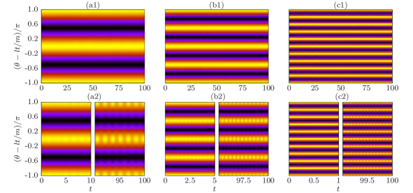
Figure 2: Evolution of some non-spreading wave packets under the influence of residual interaction noise. Under weak interaction noise with strength $g_{\xi}=0.002$ (figures a1-c1) the wave packets keep its shape during the evolution, while a stronger interaction noise with strength $g_{\xi}=0.05$ (figures a2-c2) will induce shape oscillation of the wave packets. Wave packet parameters are: $m=1,l=1$ for figures (a1, a2); $m=2,l=3$ for figures (b1, b2) and $m=5,l=5$ for figures (c1, c2).

In figure 2, we plot the evolution of some non-spreading wave packets (with $m,l=1,1;2,3$ and $5;5$) under the influence of residual interaction noise with both a very weak strength $g_{\xi}=0.002$ and a little stronger one $g_{\xi}=0.05$. (Here, we mean stronger compared to $g_{\xi}=0.002$. But, it is still a weak interaction in fact. The “kinetic” energy of a non-spreading wave packet is $E_{k}=-\frac{1}{2}\int_{0}^{2\pi}\psi_{ml}^{*}\frac{\partial^{2}}{\partial\theta^{2}}\psi_{ml}d\theta=l^{2}+m^{2}$, while the interaction energy is $E_{i}=\frac{g_{\xi}}{2}\int_{0}^{2\pi}|\psi_{ml}|^{4}d\theta=\frac{3g_{\xi}}{8\pi}$. Thus, for $g_{\xi}=0.05$, $E_{i}\ll E_{k}$ still holds.) In the figure, to conveniently compare the shapes of a wave packet at different times during the evolution, the vertical coordinate is set to $\phi=\theta-lt/m$, i.e., the wave packet is shifted to its initial location. From this figure, we see that for very weak noise, the non-spreading wave packet can keep its shape for quite a long time, while a stronger noise will induce a periodical breathing of the wave packet shape after long time. For both cases, the periodical travel of wave-packet in the ring is not affected by the interaction noise.

The numerically found shape breathing periods for different wave packets are listed in table 1. From the table, it is natural to conclude that breathing period is totally determined by the wave packet parameters $m$, and has nothing to do with $l$ and $g_{\xi}$, and its value is approximately $T\approx\pi/\left(2m^{2}\right)$. This oscillating period can be easily understood by considering the formation mechanism of a breathing mode. For wave packet with quantum number $m$, the interaction noise will induce a transition to state with quantum number $3m$, thus excites a breathing mode. Taking $m=1$ for an example, in figure 3, we show the formation of such a breathing mode by adding wave packet $\psi_{1}=\cos\left(\theta\right)$ and a small perturbation $\Delta\psi_{1}=\delta\cos\left(3\theta\right)\exp\left[i\varphi\right]$. When $\psi_{1}$ and $\Delta\psi_{1}$ are in phase ($\varphi=0$), the excitation will have a suppressing effect on width of the wave packet, while $\psi_{1}$ and $\Delta\psi_{1}$ have a phase difference of $\pi$ ($\varphi=\pi$), the excitation will spread the wave packet. Thus, for wave packet with quantum number $m$, the breathing period will be

$$T=\frac{2\pi}{\left(3m-m\right)^{2}}=\frac{\pi}{2m^{2}}.$$ (20)

And if there exists a considerable large interaction noise, higher order oscillating modes will be excited as shown in figure 4 where the evolution of non-spreading wave packet with $l=1,m=1$ under residual interaction noise with strength $g_{\xi}=0.5$ is plotted. The heat map is a plot of $|\psi(\phi,t)|^{2}$ with $\phi=\theta-lt/m$, and the line in the bottom panel is a plot of $|\psi(\phi=0,t)|$. From both plots, higher frequency oscillations can be easily observed after about $t=40$.

Wave packet parameters		Noise Strength	Breathing Period
$m$	$l$	$g_{\xi}$	$T$
		0.01	1.5674
1	1	0.02	1.5678	$\approx\pi/2$
		0.05	1.5678
	2	0.02	0.3934
2	3	0.05	0.3930	$\approx\pi/8$
	4	0.05	0.3932
3	2	0.05	0.1742	$\approx\pi/18$
5	5	0.05	0.0628	$\approx\pi/50$

Table 1: Shape breathing period of some non-spreading wave packets subjected to interaction noise. The values of breathing period are collected from numerical simulations, which have a perfect agreement with equation (20).

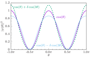
Figure 3: Schematic formation of a breathing mode excitation on the non-spreading wave packet with $m=1$. The superposition of main wave function $\psi=\cos\left(\theta\right)$ and small excitation wave function $\Delta\psi=\delta\cos\left(\theta\right)\exp\left(i\varphi\right)$ forms a breathing mode. When $\psi$ and $\delta\psi$ have the same phase, the wave packet is suppressed; while their phases are opposite, the wave packet is broadened.

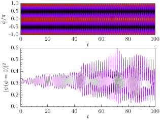
Figure 4: High order oscillating modes excited by interaction noise with a considerable large strength $g_{\xi}=0.5$. The top panel is a heat map plot of $|\psi(\phi,t)|^{2}$ with $\phi=\theta-lt/m$. The bottom panel is a plot of $|\psi(\phi=0,t)|^{2}$. The wave packet parameters are $m=1,l=1$.

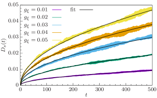
Figure 5: Shape difference evolution for non-spreading wave packet subjected to residual interaction noise with different strength. Mean values of shape difference $D_{s}\left(t\right)$ for 500 individual simulations are plotted for interaction noises with strength $g_{\xi}=0.01,0.02,0.03,0.04,0.05$ (represented by different colors as labeled in the figure). The black lines are corresponding square root function $D_{s}\left(t\right)=D_{\xi}\sqrt{t}$ fits of the data, the fitting parameters are $D_{\xi}=4.23,8.45,13.4,16.9,21.2\times 10^{-4}$ respectively. The wave packet parameters are $m=1$, $l=1$ for all lines.

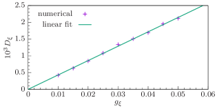
Figure 6: Shape-keeping ability of non-spreading wave packets against residual interaction noise strength. The “+” are data points of $\left(g_{\xi},D_{\xi}\right)$ obtained from numerical results. The solid line is a linear fit of the data points. The wave packet parameters are $m=1$ and $l=1$.

To quantitatively measure the shape stability of the non-spreading wave packets, we introduce the following quantity

$$D_{s}\left(t\right)=\frac{\int\left|\left|\psi\left(\theta-\theta_{c,t},t\right)\right|^{2}-\left|\psi\left(\theta,0\right)\right|^{2}\right|d\theta}{\int\left|\psi\left(\theta,0\right)\right|^{2}d\theta},$$ (21)

to describe the shape difference of wave packet between time $t$ and $0$ (initial). Here wave packet at time $t$ is shifted by $\theta_{c,t}$ (azimuthal angle the wave packet have passed since $t=0$) to line up with the initial wave packet. If $D_{s}=0$, profiles of the wave packet at time $t$ and $0$ are absolutely the same. And a larger value of $D_{s}$ indicates a bigger shape change. It is reasonable to expect that the amount of shape difference will positively relate to the strength of the interaction noise, see figure 5 where the shape differences of non-spreading wave packet with $m=1$, $l=1$ are plotted for different strength of residual interaction noises. From the figure, the numerical results also suggest a square root formula of the shape difference

$$D_{s}\left(t\right)=D_{\xi}\sqrt{t}.$$ (22)

Thus, $D_{\xi}$ can be interpreted as a parameter to describe the shape-keeping ability of the non-spreading wave packets. A larger value of $D_{\xi}$ indicates that wave packet will deviate from its initial shape more quickly, while a smaller value of $D_{\xi}$ means the wave packet will keep its initial shape for a longer time. Numerical results show a linear dependence of $D_{\xi}$ on the interaction noise strength $g_{\xi}$, see figure 6. More numerical results show that these conclusions also hold for non-spreading wave packets with other values of $m$ and $l$.

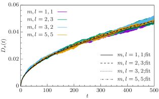
Figure 7: Shape difference evolution for different non-spreading states. Mean values of shape difference for 500 individual simulations are plotted for different states $m,l=1,1;2,3;3,2;5,5$ (represented by different colors as labeled in the figure). The black lines are the corresponding square root function $D_{s}\left(t\right)=D_{\xi}\sqrt{t}$ fits of the data, the fitting parameters are $D_{\xi}=2.09,2.16,2.18,2.14\times 10^{-3}$ respectively. The interaction noise strength is $g_{\xi}=0.05$ for all lines.

We also examined the shape differences for different non-spreading wave packets during their evolution. In figure 7, we plot the evolution of $D_{s}$ for wave packets with parameters $m,l=1,1;2,3;3,2;5,5$. As all the lines almost overlap with each other and at the same time the square root function fitting parameter $D_{\xi}=2.09,2.16,1.18,2.14\times 10^{-3}$ are very close to each other, we conclude that all the non-spreading wave packets are equally stable against residual interaction noise.

At last, we point out that the square root increasing formula (22) only holds for a small value of $D_{s}$. From the definition, the value of $D_{s}$ will never be larger than 1. Therefore, when $D_{s}$ becomes large, it will attain a saturation. In figure 8, an example is shown for parameters $g_{\xi}=0.5,m=1,l=1$. From the figure, one see that when $t<400$ formula (22) fits the data well. However, when $t>1400$ the increase of $D_{s}$ becomes saturated.

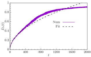
Figure 8: Saturation of shape difference. Mean values of shape difference $D_{s}$ for 500 individual simulations are plotted for wave packets $m=1,l=1$. The strength of residual interaction noise is $g_{\xi}=0.5$. The solid line is the numerical results, and the black dash line is the square root fit.

5 Conclusion

In conclusion, we examined the non-spreading wave packets in a ring. We found that there only exist one set of non-spreading wave packets in a ring, and they have been found analytically. The realization of these packets in ultra-cold atom systems (with the assistance of Feshbach resonance technique to eliminate contact interaction between atoms) is discussed. The stability of these wave packets against residual interaction noise is examined numerically. It is found that these non-spreading wave packets are stable against weak interaction noise, and a strong interaction noise will induce a periodical shape breathing of the wave packets. All these wave packets have the shape-keeping ability. And the shape-keeping ability is linearly related to the interaction noise strength.

While we focus on the non-spreading wave packet and its main features in the present work, it will also be interesting to further build a matter-wave interferometer using such non-spreading wave packets. Due to the linearity feature, the splitting and recombining processes in operating an interferometer are expected to not destroy the non-spreading property. The detailed splitting, recombining scheme, and the interference pattern may be discussed in future work. Other interesting extensions of the present work are to study the persistent current and quantum time crystal related phenomena.

References

References

- [1] Gangat A, Pradhan P, Pati G and Shahriar M S 2005 Two-dimensional nanolithography using atom interferometry Phys. Rev. A 71 043606
- [2] Fouda M F, Fang R, Ketterson J B and Shahriar M S 2016 Generation of arbitrary lithographic patterns using Bose-Einstein-condensate interferometry Phys. Rev. A 94 063644
- [3] O’Dwyer C, Gay G, de Lesegno B V, Weiner J, Camposeo A, Tantussi F, Fuso F, Allegrini M and Arimondo E 2005 Atomic nanolithography patterning of submicron features: writing an organic self-assembled monolayer with cold, bright Cs atom beams Nanotechnology 16 1536
- [4] Vengalattore M, Higbie J M, Leslie S R, Guzman J, Sadler L E and Stamper-Kurn D M 2007 High-resolution magnetometry with a spinor Bose-Einstein condensate Phys. Rev. Lett. 98 200801
- [5] Muessel W, Strobel H, Linnemann D, Hume D B and Oberthaler M K 2014 Scalable spin squeezing for quantum-enhanced magnetometry with Bose-Einstein condensates Phys. Rev. Lett. 113 103004
- [6] Cronin A D and Schmiedmayer J 2009 Optics and interferometry with atoms and molecules Rev. Mod. Phys. 81 1051
- [7] Lee C, Huang J, Deng H, Dai H and Xu J 2012 Nonlinear quantum interferometry with Bose condensed atoms Frontiers of Physics 7 109
- [8] Müntinga H, Ahlers H, Krutzik M, Wenzlawski A, Arnold S, Becker D, Bongs K, Dittus H, Duncker H, Gaaloul N, Gherasim C, Giese E, Grzeschik C, Hänsch T W, Hellmig O, Herr W, Herrmann S, Kajari E, Kleinert S, Lämmerzahl C, Lewoczko-Adamczyk W, Malcolm J, Meyer N, Nolte R, Peters A, Popp M, Reichel J, Roura A, Rudolph J, Schiemangk M, Schneider M, Seidel S T, Sengstock K, Tamma V, Valenzuela T, Vogel A, Walser R, Wendrich T, Windpassinger P, Zeller W, van Zoest T, Ertmer W, Schleich W P and Rasel E M 2013 Interferometry with Bose-Einstein condensates in microgravity Phys. Rev. Lett. 110 093602
- [9] Robins N P, Altin P A, Debs J E and Close J D 2013 Atom lasers: production, properties and prospects for precision inertial measurement Physics Reports 529 265
- [10] Bolpasi V, Efremidis N K, Morrissey M J, Condylis P C, Sahagun D, Baker M and von Klitzing W 2014 An ultra-bright atom laser New Journal of Physics 16 033036
- [11] Khaykovich L, Schreck F, Ferrari G, Bourdel T, Cubizolles J, Carr L D, Castin Y and Salomon C 2002 Formation of a matter-wave bright soliton Science 296 1290
- [12] Strecker K E, Partridge G B, Truscott A G and Hulet R G 2002 Formation and propagation of matter-wave soliton trains Nature 417 150
- [13] Strecker K E, Partridge G B, Truscott A G and Hulet R G 2003 Bright matter wave solitons in Bose-Einstein condensates New Journal of Physics 5 73
- [14] Abdullaev F K and Garnier J 2008 Bright solitons in Bose-Einstein condensates: theory Emergent Nonlinear Phenomena in Bose-Einstein Condensates: Theory and Experiment ed P G Kevrekidis, D J Frantzeskakis and R Carretero-Gonzalez (Berlin, Heidelberg: Springer Berlin Heidelberg) p 25
- [15] Martin A D and Ruostekoski J 2012 Quantum dynamics of atomic bright solitons under splitting and recollision, and implications for interferometry New Journal of Physics 14 043040
- [16] Polo J and Ahufinger V 2013 Soliton-based matter-wave interferometer Phys. Rev. A 88 053628
- [17] Gertjerenken B 2013 Bright-soliton quantum superpositions: Signatures of high- and low-fidelity states Phys. Rev. A 88 053623
- [18] Helm J L, Rooney S J, Weiss C and Gardiner S A 2014 Splitting bright matter-wave solitons on narrow potential barriers: Quantum to classical transition and applications to interferometry Phys. Rev. A 89 033610
- [19] Sakaguchi H and Malomed B A 2016 Matter-wave soliton interferometer based on a nonlinear splitter New Journal of Physics 18 025020
- [20] McDonald G D, Kuhn C C N, Hardman K S, Bennetts S, Everitt P J, Altin P A, Debs J E, Close J D and Robins N P 2014 Bright Solitonic Matter-Wave Interferometer Phys. Rev. Lett. 113 013002
- [21] McDonald G D, Kuhn C C N, Hardman K S, Bennetts S, Everitt P J, Altin P A, Debs J E, Close J D and Robins N P 2017 Erratum: Bright Solitonic Matter-Wave Interferometer [Phys. Rev. Lett. 113, 013002 (2014)] Phys. Rev. Lett. 118 219903
- [22] Fattori M, D’Errico C, Roati G, Zaccanti M, Jona-Lasinio M, Modugno M, Inguscio M and Modugno G 2008 Atom interferometry with a weakly interacting Bose-Einstein condensate Phys. Rev. Lett. 100 080405
- [23] Gustavsson M, Haller E, Mark M J, Danzl J G, Rojas-Kopeinig G and Nägerl H-C 2008 Control of interaction-induced dephasing of Bloch oscillations Phys. Rev. Lett. 100 080404
- [24] Haine S A 2016 Mean-Field Dynamics and Fisher Information in Matter Wave Interferometry Phys. Rev. Lett. 116 230404
- [25] Haine S A 2018 Quantum noise in bright soliton matterwave interferometry New Journal of Physics 20 33009
- [26] Jo G-B, Shin Y, Will S, Pasquini T A, Saba M, Ketterle W, Pritchard D E, Vengalattore M and Prentiss M 2007 Long Phase Coherence Time and Number Squeezing of Two Bose-Einstein Condensates on an Atom Chip Phys. Rev. Lett. 98 030407
- [27] Berrada T, van Frank S, Bücker R, Schumm T, Schaff J-F and Schmiedmayer J 2013 Integrated Mach-Zehnder interferometer for Bose-Einstein condensates Nature Communications 4 2077
- [28] Gross C, Zibold T, Nicklas E, Estéve J and Oberthaler M K 2010 Nonlinear atom interferometer surpasses classical precision limit Nature 464 1165
- [29] Lücke B, Scherer M, Kruse J, Pezzé L, Deuretzbacher F, Hyllus P, Topic O, Peise J, Ertmer W, Arlt J, Santos L, Smerzi A and Klempt C 2011 Twin Matter Waves for Interferometry Beyond the Classical Limit Science 334 773
- [30] Berry M V and Balazs N L 1979 Nonspreading wave packets American Journal of Physics 47 264
- [31] Hu Y, Siviloglou G A, Zhang P, Efremidis N K, Christodoulides D N and Chen Z 2012 Self-accelerating Airy beams: generation, control, and applications Nonlinear Photonics and Novel Optical Phenomena (Springer Series in Optical Sciences vol 170) ed Z Chen and R Morandotti (New York, NY: Springer New York) p 1
- [32] Siviloglou G A, Broky J, Dogariu A and Christodoulides D N 2007 Observation of accelerating Airy beams Phys. Rev. Lett. 99 213901
- [33] Voloch-Bloch N, Lereah Y, Lilach Y, Gover A and Arie A 2013 Generation of electron Airy beams Nature 494 331
- [34] Efremidis N K, Paltoglou V and von Klitzing W 2013 Accelerating and abruptly autofocusing matter waves Phys. Rev. A 87 043637
- [35] Yuce C 2015 Self-accelerating matter waves Modern Physics Letters B 29 1550171
- [36] Bouyer P 2014 The centenary of Sagnac effect and its applications: from electromagnetic to matter waves Gyroscopy and Navigation 5 20
- [37] Barrett B, Geiger R, Dutta I, Meunier M, Canuel B, Gauguet A, Bouyer P and Landragin A 2014 The Sagnac effect: 20 years of development in matter-wave interferometry Comptes Rendus Physique 15 875
- [38] Dayon D J, Toland J R E and Search C P 2010 Atom gyroscope with disordered arrays of quantum rings Journal of Physics B: Atomic, Molecular and Optical Physics 43 115302
- [39] Helm J L, Cornish S L and Gardiner S A 2015 Sagnac interferometry using bright matter-wave solitons Phys. Rev. Lett. 114 134101
- [40] Stevenson R, Hush M R, Bishop T, Lesanovsky I and Fernholz T 2015 Sagnac interferometry with a single atomic clock Phys. Rev. Lett. 115 163001
- [41] Ryu C, Blackburn P W, Blinova A A and Boshier M G 2013 Experimental realization of Josephson junctions for an atom SQUID Phys. Rev. Lett. 111 205301
- [42] Wang Y-H, Kumar A, Jendrzejewski F, Wilson R M, Edwards M, Eckel S, Campbell G K and Clark C W 2015 Resonant wavepackets and shock waves in an atomtronic SQUID New Journal of Physics 17 125012
- [43] Mathey A C and Mathey L 2016 Realizing and optimizing an atomtronic SQUID New Journal of Physics 18 055016
- [44] Kumar A, Anderson N, Phillips W D, Eckel S, Campbell G K and Stringari S 2016 Minimally destructive, Doppler measurement of a quantized flow in a ring-shaped Bose-Einstein condensate New Journal of Physics 18 025001
- [45] Beattie S, Moulder S, Fletcher R J and Hadzibabic Z 2013 Persistent currents in spinor condensates Phys. Rev. Lett. 110 025301
- [46] Ryu C, Andersen M F, Cladé P, Natarajan V, Helmerson K and Phillips W D 2007 Observation of persistent flow of a Bose-Einstein condensate in a toroidal trap Phys. Rev. Lett. 99 260401
- [47] Brand J and Reinhardt W P 2001 Generating ring currents, solitons and svortices by stirring a Bose-Einstein condensate in a toroidal trap Journal of Physics B: Atomic, Molecular and Optical Physics 34 L113
- [48] Li T, Gong Z-X, Yin Z-Q, Quan H T, Yin X, Zhang P, Duan L-M and Zhang X 2012 Space-time crystals of trapped ions Phys. Rev. Lett. 109 163001
- [49] Öhberg P and Wright E M 2018 On quantum time crystals and interacting gauge theories in atomic Bose-Einstein condensates arXiv:1812.04672
- [50] Sacha K and Zakrzewski J 2018 Time crystals: a review Reports on Progress in Physics 81 16401
- [51] Chin C, Grimm R, Julienne P and Tiesinga E 2010 Feshbach resonances in ultracold gases Rev. Mod. Phys. 82 1225
- [52] Timmermans E, Tommasini P, Hussein M and Kerman A 1999 Feshbach resonances in atomic Bose-Einstein condensates Physics Reports 315 199
- [53] Pollack S E, Dries D, Junker M, Chen Y P, Corcovilos T A and Hulet R G 2009 Extreme Tunability of Interactions in a 7Li Bose-Einstein Condensate Phys. Rev. Lett. 102 090402
- [54] Madelung E 1927 Quantentheorie in hydrodynamischer Form Zeitschrift für Physik 40 322
- [55] Lin C-L, Huang M-J and Hsiung T-C 2008 Nonspreading wave packets in a general potential V(x,t) in one dimension arXiv:0809.4105
- [56] Wright E M, Arlt J and Dholakia K 2000 Toroidal optical dipole traps for atomic Bose-Einstein condensates using Laguerre-Gaussian beams Phys. Rev. A 63 13608
- [57] Arnold A S 2004 Adaptable-radius, time-orbiting magnetic ring trap for Bose-Einstein condensates Journal of Physics B: Atomic, Molecular and Optical Physics 37 L29
- [58] Crookston M B, Baker P M and Robinson M P 2005 A microchip ring trap for cold atoms Journal of Physics B: Atomic, Molecular and Optical Physics 38 3289
- [59] W H Heathcote W H, Nugent E,Sheard B T and Foot C J 2008 A ring trap for ultracold atoms in an RF-dressed state New Journal of Physics 10, 043012
- [60] Gardiner C W 1985 Handbook of stochastic methods for physics, chemistry, and the natural sciences (Berlin, Heidelberg, New York: Springer-Verlag)