Metallicity has followed local gravitational potential of galaxies since $z=3$

Abstract

The MZ relation between stellar mass (${\rm M}_{*}$) and metallicity (Z) of nearby galaxies has been described as both a global and local property, i.e. valid also on sub-galaxy scales. Here we show that Z has remained a local property, following the gravitational potential, since $z=3$. In absorption the MZ relation has been well studied, and was in place already at $z=5.1$. A recent absorption study of GRB galaxies revealed a close match to Damped Ly$\alpha$ (DLA) galaxies, surprising due to their vastly different impact parameters and leading the authors to suggest that local metallicity follows the local gravitational potential. In this paper we formulate an observational test of this hypothesis. The test, in essence, forms a prediction that the velocity dispersion of the absorbing gas in galaxy halos, normalized by the central velocity dispersion, must follow a steep log scale slope of -0.015 dex $\rm kpc^{-1}$ as a function of impact parameter out to at least 20-30 kpc. We then compile an archival data and literature based sample of galaxies seen in both emission and absorption suitable for the test, and find that current data confirm the hypothesis out to 40-60 kpc. In addition we show that the distribution of the velocity offsets between $z_{\rm em}$ and $z_{\rm abs}$ favours a model where DLA systems are composed of individual sub-clouds distributed along the entire path through the halo, and disfavours a model where they are one single cloud with a bulk motion and internal sub-structure.

1 Introduction

The mass-metallicity (MZ) relation for galaxies is well documented and has been observed both in emission (Tremonti et al., 2004; Maiolino et al., 2008) and in absorption (Christensen et al., 2014; Augustin et al., 2018; Rhodin et al., 2018). The emission MZ relation, as originally determined from luminosity-selected galaxy samples, describes a relation between the total stellar mass (${\rm M}_{*}$) of a galaxy and its emission line metallicity (Z) determined from integrated line fluxes across the central part of the galaxy. I.e. it was discovered as a relation between global properties of the galaxies. Later studies, with improved resolution, have shown that on sub-galaxy scales similar relations govern the local metallicity in galactic discs, where it correlates with the local stellar mass density (Moran et al., 2012; Sánchez et al., 2013). Those surveys also found that metallicity gradients are ubiquitous both in the nearby universe (Sánchez et al., 2014; Belfiore et al., 2017; Sánchez-Menguiano et al., 2018) and at high redshifts (Wuyts et al., 2016).

The MZ relation of absorption selected galaxies was initially identified via a relation between the ‘velocity width’ $\Delta v_{90}$ (Prochaska & Wolfe, 1997) of the absorption lines and the absorption line metallicity ([M/H]) (Wolfe & Prochaska, 1998; Ledoux et al., 2006; Neeleman et al., 2013; Som et al., 2015). Both quantities are measured in a single pencil-beam along a sightline through the circum-galactic medium (CGM) of a galaxy, its halo and in rare sightlines through the galaxy itself. The sightline is defined by the position of an unrelated background quasar and is therefore randomly chosen. Starting with Ledoux et al. (2006) it is now customary to take $\Delta v_{90}$ to be a proxy for ${\rm M}_{*}$, and the underlying assumption is here that $\Delta v_{90}$ and [M/H], both determined locally at a random impact parameter $b$ (the projected distance between the pencil beam and the galaxy centre), are close enough to the central values that the relation is still identifiable. This assumption was vindicated by Møller et al. (2013) who determined a procedure to calibrate the $\Delta v_{90}$-[M/H] relation to an ${\rm M}_{*}$-[M/H] relation, and thereby to connect it directly to the Maiolino et al. (2008) emission MZ relation. The absorption relation includes an unknown term, $C_{[M/H]}$, describing the average difference between emission metallicity and absorption metallicity. Subsequently Christensen et al. (2014) showed that this term could be understood as a product $b\times\Gamma$, where $\Gamma=-0.022\pm 0.004$ dex kpc^-1 is the average metallicity gradient of absorption selected galaxies.

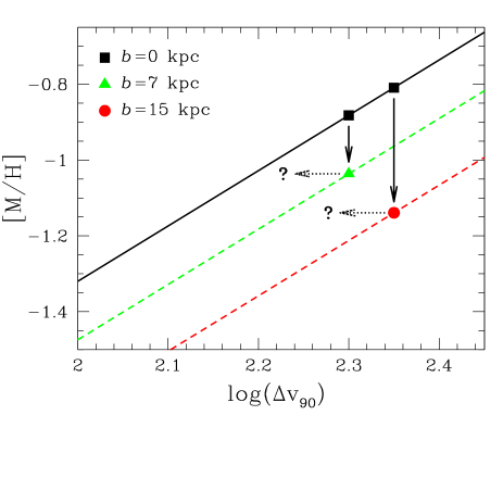
Figure 1: Simple illustration of the $\Delta v_{90}$-[M/H] relation and the effect of different impact parameters, $b$. The full black line represents a zoom on a small section of an idealized $\Delta v_{90}$-[M/H] relation with two galaxies observed at zero impact parameter (black squares). The same galaxies observed at $b$ = 7 and 15 kpc are offset to lower metallicities because of the metallicity gradient. If $\Delta v_{90}$, as assumed, is tracing the local gravitational well depth, the points would be expected also to move towards the left as illustrated by the dotted arrows.

For Damped Ly$\alpha$ (DLA) galaxies $b$ is found typically to be in the range 0-25 kpc (Krogager et al., 2017), while for sub-DLAs $b$ is typically somewhat larger (Rahmani et al., 2016; Rhodin et al., 2018). Determination of $b$ requires that the absorbing galaxy first must be found also in emission, a difficult task, and $b$ is therefore known for only a tiny fraction of the known DLAs/sub-DLAs. The random and unknown value of $b$ for the majority of the absorbers, combined with the metallicity gradient, result in a corresponding range of unknown offsets towards lower metallicities in the $\Delta v_{90}$-[M/H] relation. For example a DLA at $b=10$ kpc will on average have a measured metallicity $10\times 0.022~{}{\mathrm{d}ex}=0.22~{}{\mathrm{d}ex}$ lower than the central metallicity, potentially shifting the entire relation to lower metallicities and adding an extra scatter reflecting the range of possible values of $b$. This was thought to be the source of some of the residual scatter present in the relation: $\sigma_{\rm scatter}$([M/H]) = 0.38 (Møller et al., 2013); rms([M/H]) = 0.37 (Neeleman et al., 2013).

The effect of observing a galaxy at two different impact parameters is graphically illustrated in Fig. 1. The green and red dashed lines show how an idealized relation through the galaxy centres (full black line) is offset towards lower metallicities for increasingly larger values of $b$. As mentioned above, $\Delta v_{90}$ has been used as a proxy for galaxy mass because it was thought it would trace the depth of the gravitational potential encountered. However, at larger $b$ only the outer part of the potential well depth will be probed by the sightline. Will this then also modify the relation? A sample of DLAs with zero, or very small, impact parameters would be needed to answer this question. Gamma Ray Bursts (GRBs) provide pencil-beam line absorption data much like those of QSOs and their spectra usually contain a DLA intrinsic to the host. GRB-DLAs have much smaller impact parameters (in a sample study Lyman et al. (2017) determined a median of $b=1.0\pm 0.2$ kpc) and as the GRB afterglow fades away, the host galaxy light is not contaminated by an extremely luminous source. While the geometry for GRB host DLAs is slightly different (they only have half the sightline compared to intervening DLAs), the smaller impact parameter does make the comparison interesting.

Arabsalmani et al. (2015) analyzed a sample of GRB-DLAs with the goal to compare the GRB-DLA $\Delta v_{90}$-[M/H] relation to that of QSO-DLAs. Quite surprisingly they reported that there was no offset between the two relations, i.e. the offset between the black line and the red dashed line in Fig. 1 was not seen. As explanation they suggested that perhaps the real underlying relation is directly between [M/H] and potential well depth, i.e. that the relation is local rather than global (see their Fig. 2 and 4). If that is the case then $\Delta v_{90}$ will decrease with the exact rate to compensate the drop in metallicity as $b$ increases. Graphically a decrease in $\Delta v_{90}$ is shown as the dotted arrows in Fig. 1. If the relation is local then the dotted arrows will continue left to the point where they again intersect the black ($b=0$) relation. In other words galaxies will move along the relation, rather than across it, as $b$ changes, explaining why the relation is so easily detectable despite the unknown impact parameters. If the suggestion can be confirmed, then this will lend strong support to the reports of local MZ relations in resolved studies of nearby (out to $z=0.05$) galaxy discs. Even more importantly it will extend those results out to high redshifts and to sightlines far outside the visible parts of galaxies.

The result by Arabsalmani et al. (2015) cited above effectively suggests a relation based on two bins; one defined by the average impact parameter of GRB-DLAs, and another defined by the average impact parameter of QSO-DLAs. The lack of knowledge of the individual impact parameters prevented the authors of that paper from confirming that the relation exists. In this paper we aim to perform a direct test of the hypothesis that the $\Delta v_{90}$-[M/H] relation is the result of a more fundamental local relation between the potential well depth and the metallicity, both measured via neutral absorbing gas in the CGM of a complete literature sample of DLAs and sub-DLAs. In Christensen et al. (2019) we will elaborate further on the radial dependence and compare to a set of dark matter (DM) halo profile models.

2 Sample properties

2.1 Sample definition

For our test we require a sample of spectroscopically confirmed galaxy counterparts to DLAs and sub-DLAs for which 4 parameters are known: $\sigma_{\mathrm{e}m}$, $b$, $\Delta v_{90}$ and $N($H i) representing the Gaussian $\sigma$ of emission lines integrated over the host galaxy, impact parameter, absorption line width and column density of neutral Hydrogen in the absorption sight-line respectively. Implicitly this also means that we know $z_{\rm em}$ and $z_{\rm abs}$ for each galaxy and each absorber. Early emission line searches for DLA galaxies in emission were primarily aimed at detection of Ly$\alpha$ because the majority of known DLA systems had redshifts $z>1.7$, where Ly$\alpha$ is shifted into the optical wavelengths and ground based optical observations therefore allowed extensive searches. However, because of its resonant nature Ly$\alpha$ was found to be poorly suited for dynamical studies of the hosts. In this work we only consider H$\alpha$, H$\beta$, $[$Oii$]$ and $[$Oiii$]$ emission lines. With current instruments those can now be found over a wide redshift range.

Table 1: QSO-DLA sample. Detailed referencing and account for the origin of each entry in the table is provided in Appendix A where we also provide the background quasar SDSS IDs. $z_{\rm abs}$ denotes the redshift of the absorber and we use $z_{\tau 50}$ when that is available. $z_{\rm em}$ is the redshift of the host galaxy measured from Balmer or Oxygen emission lines.

ID	$z_{\rm abs}$	$z_{\rm em}$	$\log N($H i)	b	$\log({\rm M}_{*}/{\rm M_{\odot}})$	$\sigma_{\mathrm{e}m}$	$\Delta v_{90}$	$v_{\rm rel}$	Metallicity	Refs.‡
				kpc		${\rm km\,s^{-1}}$	${\rm km\,s^{-1}}$	${\rm km\,s^{-1}}$	[X/H]†	[X/H]
0151+045	0.1602	0.1595	19.48	18.5	$9.73\pm 0.04$	$50\pm 20$	152	$+180$	$-0.04\pm 0.15$	(1)
2328+0022	0.65179	0.65194	20.32	11.9	$10.62\pm 0.35$	$56\pm 24$	92	$-27\pm 11$	$-0.52\pm 0.17$	(2)
1323-0021	0.71612	0.7171	20.4	9.1	$10.80^{+0.07}_{-0.14}$	$101\pm 14$	141	$-171\pm 12$	$+0.40\pm 0.3$	(3)
1436-0051A	0.7377	0.73749	20.08	45.5	$10.41\pm 0.09$	$99\pm 25$	71	$+36$	$-0.05\pm 0.12$	(4)
0153+0009	0.77219	0.77085	19.70	36.6	$10.03^{+0.18}_{-0.08}$	$121\pm 8$	58	$+227$	-
0152-2001	0.77980	0.78025	19.10	54.	-	$104\pm 13$	33	$-78$	-
1009-0026	0.8866	0.8864	19.48	39.	$11.06\pm 0.03$	$174\pm 5$	94	$+32$	$+0.25\pm 0.06$	(5)
1436-0051B	0.9281	0.92886	$18.4$	34.9	$10.20^{+0.11}_{-0.08}$	$33\pm 11$	62	$-118$	$-0.05\pm 0.55$	(6)
0021+0043	0.94181	0.94187	19.38	86.	-	$123\pm 11$	139	$-9\pm 5$	$+0.42\pm 0.15$	(7)
0302-223	1.00945	1.00946	20.36	25.	$9.65\pm 0.08$	$59\pm 6$	61	$-1$	$-0.54\pm 0.13$	(2)
2352-0028	1.03197	1.032	19.81	12.2	$9.4\pm 0.3$	$125\pm 6$	164	$+40\pm 5$	$+0.17\pm 0.13$	(8)
2206-1958	1.919991	1.9220	20.67	8.4	$9.45\pm 0.30$	$93\pm 21$	136	$-210$	$-0.60\pm 0.05$	(9)
1228-1139	2.19289	2.1912	20.60	30.	-	$93\pm 31$	163	$+159$	$-0.22\pm 0.10$	(2)
1135-0010	2.2066	2.207	22.10	0.8	-	$53\pm 3$	168	$-20\pm 10$	$-1.06\pm 0.10$	(10)
2243-6031	2.3298	2.3283	20.67	26.	$10.1\pm 0.1$	$158\pm 5$	173	$+135\pm 12$	$-0.91\pm 0.05$	(9)
2222-0946x	2.3542	2.3537	20.65	6.3	$9.62\pm 0.12$	$49.0\pm 1.6$	174	$+42\pm 30$	$-0.53\pm 0.07$	(11)
0918+1636-1x	2.412	2.4128	21.26	$<2.$	-	$21\pm 5$	344	$-38\pm 25$	$-0.66\pm 0.24$	(12)
1439+1117	2.41802	2.4189	20.10	39.	$10.74\pm 0.17$	$303\pm 12$	338	$-77$	$+0.20\pm 0.11$	(13)
0918+1636-2	2.5832	2.58277	20.96	16.2	$10.33\pm 0.08$	$107\pm 10$	288	$+36\pm 20$	$-0.19\pm 0.05$	(14)
2358+0149	2.97919	2.9784	21.69	11.8	-	$47\pm 9$	135	$+60$	$-1.90\pm 0.18$	(15)
2233+1318	3.14930	3.15137	20.00	19.5	$9.85\pm 0.14$	$23\pm 10$	228	$-150$	$-0.97\pm 0.13$	(16)

We carefully searched the literature for all such systems and have compiled a complete literature sample of 21 absorption selected galaxies with the required information (Table LABEL:tab:sample). For several of the objects in Table LABEL:tab:sample not all the required parameters had been extracted from the data in the original papers. For those we reprocessed the original (or supplementary) data as detailed in Appendix A, where we also provide references to the original publications. One additional parameter (the stellar mass, ${\rm M}_{*}$) is also relevant for the present purposes. When available we have also recorded this in Table LABEL:tab:sample. The sample has been collected from programmes utilizing a wide range of instrumentation, observing strategies and reduction techniques each adapted to fit the wide range of purposes and goals of the original studies. The original publication formats of those data are therefore very inhomogeneous, and it has been necessary to re-process several observables into a homogeneous data-set.

Our sample is well spread over the observable parameter space and in order to assess dependencies on the various parameters we shall therefore also consider sub-samples as defined here. In total our sample contains 11 hosts at $z_{\rm em}$ below 1.05 (the low redshift sample) and 10 hosts at $z_{\rm em}$ above 1.90 (the high redshift sample). It contains 11 DLAs (the DLA sample), 9 sub-DLAs and 1 absorber with even slightly lower $\log N$(H i). We shall refer to the 10 low $\log N$(H i) hosts together as the “sub-DLA” sample. Unfortunately there is a strong tendency for DLAs and sub-DLAs in our sample to cluster in the ‘high redshift’ and ‘low redshift’ sample respectively. This causes some degeneracy regarding dependency on $z$ and $\log N$(H i).

For 15 of the hosts there are stellar masses known from SED fitting. For 7 of those $\log({\rm M}_{*}/{\rm M_{\odot}})$ is in the range $9.4-10.03$ (the low mass sample), the other 8 have $\log({\rm M}_{*}/{\rm M_{\odot}})$ in the range $10.1-11.06$ (the high mass sample).

Historically the offset between $z_{\rm abs}$ and $z_{\rm em}$ was used as the first tracer of the dynamical relation between the host galaxy and its CGM (e.g. Warren & Møller, 1996; Christensen et al., 2005), but its use was complicated by the lack of a unique definition of $z_{\rm abs}$. Most DLA absorbers have complex multi-component structures spanning in excess of 100 ${\rm km\,s^{-1}}$ or even several times that, and some convenient value within this range has often simply been chosen. Until now there has been no strong motivation to formulate a unique definition. With a rapidly increasing sample size of DLA galaxies with well defined emission redshifts this situation has changed. A useful definition should represent a well defined “average” of the complex and since the other absorption related dynamical tracer ($\Delta v_{90}$) is formed by cuts in the distribution of optical depth of the low-ion phase, we shall here follow Møller et al. (2018) and use (where possible) the redshift of median optical depth ($z_{\tau 50}$), i.e. the redshift where there is 50% of the low-ion optical depth on either side. We then define the relative velocity offset ($v_{\rm rel}$) as ($z_{\rm abs}-z_{\rm em}$) converted to velocity, i.e. it is positive when the absorption occurs at higher redshift than the emission.

To obtain a uniform set of impact parameters, $b$, we extract those in arcsec from the original papers and convert them to kpc assuming a flat cosmology with $H_{0}=70.4$ ${\rm km\,s^{-1}}$ Mpc^-1, $\Omega_{\Lambda}=0.727$ (Komatsu et al., 2011). In this cosmology, a 1-arcsec transverse separation on the sky corresponds to 7.6 kpc at $z=0.8$ and 8.3 kpc at at $z=2.4$.

For reference we also, in column (10) of Table LABEL:tab:sample, list absorption metallicities when available. In order to obtain a homogeneous sample we have searched the literature for the measured total metal column densities and have then computed metallicitites based on solar abundances given in Asplund et al. (2009). In particular we also use the choices used by De Cia et al. (2016) (their Table 1). We only consider metallicities based on Zn, S and Si as provided in the references listed in column (11) of Table LABEL:tab:sample. Metallicities of our sample span the range from $-1.90\pm 0.18$ to $+0.42\pm 0.15$ i.e. 2.3 dex.

2.2 The DLA galaxy selection function

Any sample of high redshift galaxies contains intrinsic biases which are a function of the exact way the galaxies are identified. The selection function of DLA galaxies contains three components. First there is the selection of the DLA absorption line which is a selection via H i absorption cross-section. The probability that a given galaxy is selected as absorber scales directly with the area that the DLA gas of that galaxy covers on the sky and that area scales, via the Holmberg relation, with the luminosity of the galaxy resulting in a flat selection function over a wide span of luminosities (see figure 10 of Krogager et al., 2017). This is in sharp contrast to luminosity selected galaxy samples which, by construction, have a luminosity cutoff. Other than the cross-section weighting, the selection of the individual DLAs forms a random sampling onto any scaling relation (e.g. MZ and $\Delta v_{90}$-[M/H] relations).

The second component of the selection function is the method by which one seeks to detect emission from the host. The first successfully used methods were the Ly$\alpha$ narrow band imaging technique (Møller & Warren, 1993) and the Lyman Break broad band imaging selection (Steidel et al., 1995). HST imaging with follow-up spectroscopy of candidates (e.g. Le Brun et al., 1997; Warren et al., 2001) and later both optical and IR IFUs (e.g. PMAS (Christensen et al., 2007) and SINFONI (Péroux et al., 2011a)) were used. Latest, also ALMA has proven to be a powerful tool to identify hosts via molecular emission lines (Neeleman et al., 2016; Klitsch et al., 2018). In an interim period, before the advent of the new generation of powerful data-cube instruments, a single slit triangulation method was used with significant success (Møller et al., 2004; Fynbo et al., 2010; Krogager et al., 2017). Each method has its limitations, notably in terms of the field covered.

The last component of the selection is the target selection. Initially the selection of targets was either random or designed to cover the known parameter space evenly (see e.g. figure 1 of Warren et al., 2001). Later it was shown that luminosity scales with metallicity of the DLA, and that it therefore is more telescope time efficient to only select DLAs above a given metallicity threshold since they are likely to have brighter hosts. Such a biasing towards higher metallicity in some of the later samples is equivalent to a normal luminosity bias, i.e. it skews the underlying flat selection towards mostly brighter galaxies. As above, this does not affect the random sampling of the underlying scaling relations, it simply means that just like for flux limited galaxy samples, only the brighter end of the relations are studied. The shape of the relations will not be biased. However, the target does need to be inside the field of view (FOV) of the observation in order to be detected.

For all surveys based on imaging and IFU cubes with sufficiently large field, the target will always be inside the FOV. Surveys which only partly cover the possible impact parameter range, e.g. slit triangulation, will inherently contain an additional bias towards more easily finding hosts at smaller impact parameter and maybe missing hosts at larger impact parameter. Scaling relations containing impact parameter could be affected by such a detection bias. In our sample such a bias is only present for the two hosts identified via the X-shooter triangulation survey (0918+1636-1 and 2222-0946). A third host (0918+1636-2) was not in the targeted sample of that survey but was identified serendipitously during the search for the lower redshift host. The two sample members are marked in Table LABEL:tab:sample. The strength of the effect was computed by Fynbo et al. (2010) who find that “slightly above 90 per cent of the galaxy centres are covered by at least one slit”. Therefore, in the complete triangulation survey (10 targets), less than 1 host is expected to be missed due to large impact parameter. In our sample defined here the effect is $0.2$ target and therefore negligible.

3 Results

3.1 Mass-metallicity relation, local or global?

The first question we examine is the hypothesis that the metallicity measured along a pencil beam is related to how deep the sightline dips into the gravitational potential, rather than to the total stellar mass of the galaxy (as illustrated by the sightline trace in Figure 4 of Arabsalmani et al., 2015). In order for this to explain why GRB-DLAs and QSO-DLAs follow exactly the same relation, despite their vastly different distribution on impact parameters, there must be a gradient of $\Delta v_{90}$ outwards through the galaxy halo which exactly cancels the metallicity gradient (as illustrated in Fig. 1). The metallicity gradient for DLA galaxies has been reported as $\Gamma=-0.022\pm 0.004$ dex kpc^-1 (Christensen et al., 2014) and $\Gamma=-0.022\pm 0.001$ dex kpc^-1 (Rhodin et al., 2018), and the gradient of [M/H] vs log($\Delta v_{90}$) is 1.46 (Ledoux et al., 2006; Møller et al., 2013). In order to cancel each other out the gradient of log($\Delta v_{90}$) should be $-0.022/1.46=-0.015$ dex kpc^-1. The above forms a strong prediction which is based on a sample of 110 QSO-DLAs (Møller et al., 2013) and a sample of 16 GRB-DLAs (Arabsalmani et al., 2015). If our present, independent, sample is found to follow this prediction, then the result from those three samples taken together makes a strong case in favour of the tested hypothesis.

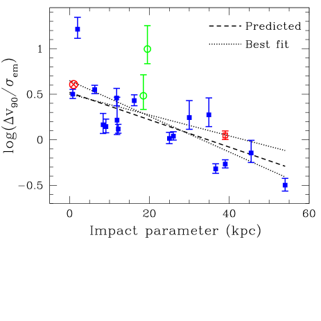
Figure 2: Local dynamical state of the halo gas ($\Delta v_{90}$) normalized to the central value of $\sigma_{\mathrm{e}m}$, as a function of $b$ (blue squares). The green open circles are objects where the emission line region is offset by a few kpc from the galaxy centre and where $\sigma_{\mathrm{e}m}$ consequently could underestimate the central velocity dispersion. The red open square is AGN dominated. The black dashed line is the hypothesis being tested while the two dotted lines are two fits to the data (see text). The red circle with an X is the average point for GRB-DLAs and was not included in the fits.

If we take $\sigma_{\mathrm{e}m}$ to be a measure of the central velocity dispersion of the gas, then we can use this to normalize $\Delta v_{90}$ for each pencil beam absorber. In Fig. 2 we therefore plot log($\Delta v_{90}$ / $\sigma_{\mathrm{e}m}$) vs. $b$ (blue squares), as well as the line with a slope of $-0.015$ and intercept = $0.517$ (black dashed line) which is the prediction we test. The two dotted lines are the minimum $\chi^{2}$ fit linear relations. For a better visual impression we have limited the plot to the inner 60 kpc but there is an additional single object at $b=86$ kpc (see Fig. 3). The two dotted lines in Fig. 2 are fits including (slope of $-0.011$) and excluding (slope of $-0.020$) this extra-large impact parameter object. The two green points are objects for which we know that the emission line region is offset from the centre of the galaxy by 3.8 and 2.1 kpc (for 0151+045 and 2233+1318 respectively, details provided in Appendix A) and that they therefore could be representing gas in smaller star-forming regions rather than the entire galaxy. I.e. they might provide an under estimate of the globally integrated $\sigma_{\mathrm{e}m}$, and as such could then become upwards outliers. In the figure one green point is seen to follow the general distribution while the other lies far above it. The $\sigma_{\mathrm{e}m}$ of the outlier, 2233+1318, is also found to be unusually low compared to the stellar-mass Tully-Fisher relation (Christensen & Hjorth, 2017), but we shall here conservatively keep both in the sample. The open red square is an AGN dominated DLA host (1439+1117, see Appendix A), and in the paper reporting the discovery of this host Rudie et al. (2017) argue that the absorbing gas in this case is the result of an AGN driven outflow. It is of great interest to test if, in such cases, the kinematic properties of the absorber are dominated by the outflow mechanism - or if they are tracing the gravitational potential regardless of the outflow origin. It is seen that this DLA lies precisely on the relation of the potential well hypothesis.

We can obtain an additional point at small impact parameter if we also consider GRB-DLAs. A complete literature sample of 10 GRB-DLAs with the required dynamical parameters $\Delta v_{90}$ and $\sigma_{\mathrm{e}m}$ was presented in Arabsalmani et al. (2018). We do not know the exact impact parameters for each, but GRB impact parameters are always small. Here we simply compute the average $\mbox{$\Delta v_{90}$}/\mbox{$\sigma_{\mathrm{e}m}$}$, and use the median impact parameter ($1.0\pm 0.2$ kpc) found by Lyman et al. (2017). One of the objects of that sample (GRB 090323A) has an extremely large $\Delta v_{90}$ of 843 ${\rm km\,s^{-1}}$, more than twice that of any object in our QSO-DLA sample. In a separate study Savaglio et al. (2012) conclude that this system is caused by two separate galaxies and for this reason we have removed this object before computing the average. The average $\log(\mbox{$\Delta v_{90}$}/\mbox{$\sigma_{\mathrm{e}m}$})$ of the remaining 9 is $0.61\pm 0.06$ which is included in Fig. 2 as a red circle with an X. It was not included in the computation of the fits shown as dotted lines. Including all 10 GRB-DLA in the average gives instead $0.70\pm 0.08$ which would lie only insignificantly higher in the plot.

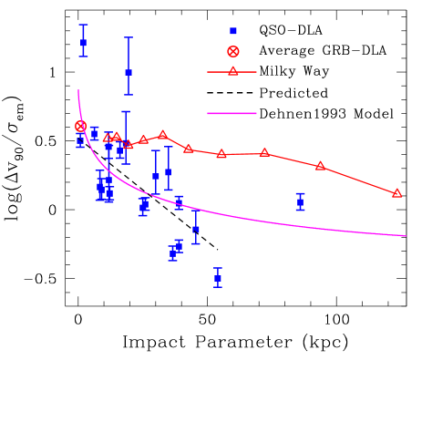
Figure 3: Average projected velocity dispersion profile of our absorption selected sample (solid blue squares) compared to the projected velocity dispersion profile of our own galaxy (open red triangles). Predicted slope and average GRB-DLA are included as in Fig. 1. We also include an example model curve from Dehnen (1993). DLA potentials are seen to be better represented by steeper potentials than the MW.

It is immediately clear from Fig. 2 that the points, out to an impact parameter of 60 kpc, follow the predicted slope well. From this we conclude:

1. there is an outward negative gradient of log($\Delta v_{90}$ / $\sigma_{\mathrm{e}m}$)

2. the slope of that gradient is in excellent agreement with the hypothesis that this is the cause of the reported lack of difference between the $\Delta v_{90}$-[M/H] relations of QSO-DLAs and GRB-DLAs

3. the implication is that the MZ relation exists locally, i.e. that both metallicity and $\Delta v_{90}$ follow the local gravitational potential. In particular we find that this is true all the way back to $z=3.1$, and out to larger distances than enclosed by galaxy disks.

In this section our aim was to test if our sample confirms the prediction of the previous, independent samples. In Sect. 4.2 we shall return with a full mathematical outline of our current understanding of the $\Delta v_{90}$-[M/H] relation and in particular determine the observed $\Delta v_{90}$ gradient, $\Gamma_{\Delta v90}$.

3.2 Absorption pencil beams: dynamical tracers of halo potentials

Figure 4: Histograms of the distribution of $v_{\rm rel}$. Left panel shows that of the entire sample, middle and right panels present two different cuts on the sample.

In the previous section we have shown that the normalized $\Delta v_{90}$ of a sample of DLA galaxies provide insight into the gravitational well profiles of their halos, and by inversion, into their matter density profiles. Before we exploit this further, the sample as reproduced in Fig. 2 deserves a few words of clarification. The figure is a representation of the projected velocity dispersion profile of the average potential well of the galaxies in our sample. Each point represents the relative drop in projected velocity dispersion from the centre to the given impact parameter, but they are all measured in separate halos. If all those galaxies were embedded in dark matter halos of vastly different profile steepness, then those differences would be expected to result in a large scatter of the individual points. For the fits shown in Fig. 2 we used a method which simultaneously determines the minimum $\chi^{2}$ fit and the internal scatter of the data (Møller et al., 2013). The resulting scatter around the simple linear fit is $0.26$ and $0.31$ excluding and including the absorber at $b=86$ kpc respectively. This scatter is small compared to the full span of the data points which is 1.7 dex, indicating that absorption selected galaxies have DM halos with similar circum-galactic profile slopes.

In Fig. 3, for comparison, we plot the projected velocity dispersion for an example potential computed from the generalized model by Dehnen (1993). This model has two scaling parameters ($a$, the scaling radius, and $\gamma$ describing the inner slope of the central density profile) and it includes both the Jaffe (1983) and the Hernquist (1990) models as special cases. A rigorous and comprehensive discussion of our DLA sample in the framework of those model potentials is presented in Christensen et al. (2019). Here we only point out that the simplifying linear approximation we applied in the previous section to investigate and resolve the relation between metallicity and potential is well justified out to an impact parameter of 40-50 kpc. In that inner CGM range the difference between the linear prediction and the Dehnen (1993) model is well within the scatter (0.26 dex). The single sub-DLA point at large impact parameter is clearly in disagreement with an extrapolation of the approximated inner CGM linear slope, but it is in good agreement with the Dehnen (1993) model at larger distances. A sample of securely verified absorber/host pairs at larger impact parameters is required to address the question of the outer halo potential. For now we conclude that DLA galaxies in general have similar density profile slopes in the inner CGM, and that they likely are flattening at larger radii as predicted by models.

Also in Fig. 3 we plot the projected velocity dispersion profile of the Milky Way Galaxy (MW) from Battaglia et al. (2005) (red triangles) together with the DLA/sub-DLA data. To ease the comparison we have normalized the MW data to its central value the same way we have normalized our absorber sample. In the representation here there is a significant difference between the MW halo and those of most of the DLA galaxies. This difference is related to differences in scaling radii and is addressed in detail by Christensen et al. (2019).

3.3 Sub-structure within, and distribution of, DLA absorbing clouds

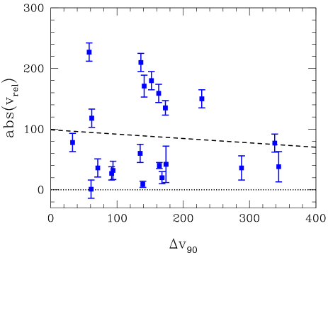
Figure 5: Here we test if abs($v_{\rm rel}$) correlates with $\Delta v_{90}$. A min-$\chi^{2}$ fit (dashed black line) finds a weak anti-correlation, but the data are fully compatible with a slope of zero and no correlation.

In Table LABEL:tab:sample we also record $v_{\rm rel}$, the emission vs. absorption velocity difference, which we defined as positive in case the absorption has the higher redshift. Let us consider two simple, opposing views of the absorbing clouds. First, one could imagine that an absorber is a single unity which has a bulk motion velocity, and within which the individual sub-components reflect random motions relative to this bulk motion. In this case $v_{\rm rel}$ represents the bulk motion and we would expect it to roughly trace the halo potential, i.e. on average it should be larger at small impact parameters and smaller further out. The velocity width $\Delta v_{90}$ would then be an intrinsic property of the complex and would not be strongly coupled to the halo potential. The other simplified view is that all the individual sub-components of a DLA system represent independent absorbing clouds spread along the pencil beam through the halo. In this case the combined velocity width of the complex ($\Delta v_{90}$) should be strongly coupled to the potential, and $v_{\rm rel}$ would simply represent the average of the ensemble, i.e. it would be stochastic of nature and should not be strongly linked to the potential.

All values of $v_{\rm rel}$ in our sample fall in the range $-210$ to $+227$ ${\rm km\,s^{-1}}$ and in Fig. 4, left panel, we show the histogram of their distribution. Half of the velocities are within a narrow range of $\pm 50$ ${\rm km\,s^{-1}}$, the other half has a flat distribution over the full range $\pm 220$ ${\rm km\,s^{-1}}$. The distribution is symmetric around zero. In the middle and right panels we use cuts on the sample to test if any obvious evidence is at hand for a coupling to the halo potential. DLAs are known to typically be closer to their host galaxies while sub-DLAs typically are found at larger distances, so indirectly this cut traces inner vs outer halo. We also make a cut directly on the impact parameter at $b=20$ kpc. In case $v_{\rm rel}$ would follow the potential we would expect the central peak of the distribution to be higher, and the distribution to be narrower, in the right panel than in the middle panel. The sample size is very small and at present all of the DLA, sub-DLA, inner and outer samples are statistically consistent with being identical. There is certainly no evidence that the peak around $\pm 50$ ${\rm km\,s^{-1}}$ is stronger in the outer parts (rightmost panels).

In the previous sections we have shown that $\Delta v_{90}$ is strongly linked to the potential, so we can make an additional test and ask the question if $v_{\rm rel}$ is positively correlated with $\Delta v_{90}$. For this we consider the absolute value, abs($v_{\rm rel}$), and in Fig. 5 we plot this against $\Delta v_{90}$. We only have errors for 9 of the 21 values in Table LABEL:tab:sample, but redshifts are in general easy to determine, so we do not expect any of the errors to be large. Of the 9 values we determine the median error to be 12 ${\rm km\,s^{-1}}$, so for the purpose of Fig. 5 we assign an error of $\pm 15$ ${\rm km\,s^{-1}}$ to the remaining 12. A minimum $\chi^{2}$ fit results in a weak negative slope of $-0.072$ (dashed line in Fig. 5) for an intrinsic scatter of 67 ${\rm km\,s^{-1}}$. The data are also fully consistent with a slope of $0.0$, i.e. with no correlation.

We conclude that $v_{\rm rel}$ of our sample is symmetrically distributed between extremes of $\pm 220$ ${\rm km\,s^{-1}}$ but 50% of the sample is found inside a narrow range of $\pm 50$ ${\rm km\,s^{-1}}$. Contrary to $\Delta v_{90}$, $v_{\rm rel}$ does not correlate strongly with the halo potential. In terms of our simple, idealized DLA model, those results favour that the multi-component structure of DLAs represent ensembles of independent absorbers spread widely along the pencil beam through the halo. In our data we cannot directly measure the path length along which the absorbers are distributed, but in figures 3 and 6 of Bird et al. (2015) it is seen that simulations of DLAs show how sub-components are distributed through the halo and that the physical path length scales directly with $\Delta v_{90}$ in agreement with our conclusion. This also means that other properties of the DLAs, such as e.g. average metallicity and distribution of metallicity on individual sub-components, represent the averages and distributions taken through the entire halo.

3.4 Dependence on redshift and/or H i column density

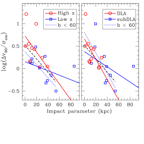
Figure 6: Comparison of sub-samples as defined in Sect. 2.1. Left: Low redshift (blue squares and full line) vs. high redshift (red circles and full line). Right: Low column density (blue) vs. high column density (red). In both panels it is seen that the red points and fits follow a steeper potential than the blue. However, excluding the single point at $b=86$ kpc (blue dotted lines) the red and blue slopes are seen to agree well.

As described in Sect. 2.1 there are some ‘natural cuts’ on our sample which can be used to obtain a first gauge of possible parameter dependencies. First, for observational reasons (space vs. ground based access to Ly$\alpha$) there is a natural division into a low and a high redshift sample: $z_{\rm em}$ below 1.05 (11 hosts) and $z_{\rm em}$ above 1.90 (10 hosts). The two sub-samples are shown in Fig. 6, left panel. The dashed black line is again the same as in previous figures, while the two full lines represent the best fit to the individual sub-samples. It is seen that the high redshift sample favours a steeper potential while the low redshift sample favours a flatter. However, recalling that the model DM halo profile shown in Fig. 3 shows strong flattening at impact parameters larger than 40-60 kpc, we repeat the fit now excluding the single point at $b=86$ kpc, and show the fit as the dotted blue line. The slopes of the full red and dotted blue lines are now seen to be in very good agreement. In the right panel we plot the DLA sample (red) and the sub-DLA sample (blue). The conclusion here is identical to that of the left panel; when we exclude the $b=86$ kpc point we find an excellent agreement between the low and high column density points.

In conclusion there is no evidence for neither redshift dependence, nor H i column density dependence, of the steepness of the inner CGM slope (here taken to mean the average slope out to a radius of 50 kpc) in DLA galaxy halos. On the contrary the evidence is that they are very similar across those two parameters.

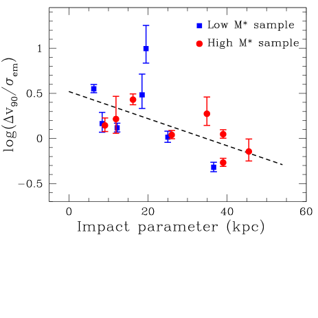
Figure 7: As Fig. 2 but here only the 15 galaxies for which the stellar mass is known. Both the low (blue squares) and the high (red dots) stellar mass sub-samples are seen to lie on the same relation.

3.5 Dependence on stellar mass

In Figures 2 and 3 we used $\sigma_{\mathrm{e}m}$ to normalize the $\Delta v_{90}$ measurements. Since $\sigma_{\mathrm{e}m}$ is known to scale with ${\rm M}_{*}$ (Christensen & Hjorth, 2017) this normalization takes out the stellar mass to first order. However, in case galaxies of different mass would sit in potentials with very different slopes, this could still be visible as a secondary effect. For this reason we show, in Fig. 7, a figure similar to Fig. 2 only here we plot the low mass sub-sample as blue squares and the high mass sub-sample as red dots (all sub-samples are defined in Sect. 2.1). Low mass galaxies are in general smaller than galaxies with higher mass, so it is unsurprising that we find a trend that lower mass galaxies in general are found to have smaller impact parameters than the higher mass galaxies. There may be a weak trend suggested that the low mass galaxies have steeper slopes than high mass galaxies but a larger sample is required in order to make a statistically valid statement about this. At present the two sub-samples are consistent with following the same relation to within the scatter.

4 Discussion

4.1 The detailed $\Delta v_{90}$-[M/H] relation

We are now able to piece together all of the various dependencies that go into the seemingly simple relation between metallicity and $\Delta v_{90}$, a relation which was first reported by Wolfe & Prochaska (1998) who interpreted it as due to rapidly rotating disks with metallicity gradients. Ledoux et al. (2006) enlarged the sample size to 70 and suggested instead that the relation was an absorption based version of the MZ relation, a suggestion confirmed by Christensen et al. (2014) who identified both the underlying MZ relation, but who also observationally confirmed the existence of a metallicity gradient. Ledoux et al. (2006) further found evidence for an evolution with redshift, and in this paper we have now shown that also the $\Delta v_{90}$ parameter displays a negative radial gradient. Here we will formulate all this into a single description.

We start by considering a sightline through the centre of a galaxy. Such a sightline will have $b=0$ and it will measure the central values of the metallicity and $\Delta v_{90}$ which we will name [M/H]_c and $\Delta v_{90,c}$ respectively. We can then write the $\Delta v_{90}$-[M/H] relation for sightlines through the centres of galaxies as

$${\rm[M/H]_{c}}=\alpha_{0}\log(\Delta v_{\rm 90,c})+\beta$$ (1)

Equation 1 is valid at $z=0$, but for a given $\Delta v_{90}$ the metallicity of the galaxy was lower in the past. Møller et al. (2013) and Neeleman et al. (2013) provide expressions for that redshift evolution but here we shall simply represent the evolution by a generic function $ze(z)$, and

$${\rm[M/H]_{c,z}}=\alpha_{0}\log(\Delta v_{\rm 90,c})+\beta-ze(z)$$ (2)

is then valid for sightlines through centres of galaxies at any redshift. In order to generalize this further to a sighline at non-zero impact parameter $b$ we follow Christensen et al. (2014) and write

$${\rm[M/H]=[M/H]_{c}+\Gamma_{\rm[M/H]}}~{}b$$ (3)

for the dependence of metallicity on the radial distance, and similarly we write

$$\log({\rm\mbox{$\Delta v_{90}$}})=\log(\Delta v_{\rm 90,c})+\Gamma_{\Delta v90}~{}b$$ (4)

for the dependence of velocity dispersion on the radial distance. Combining equations 1 through 4, and assuming that the two gradients $\Gamma_{\rm[M/H]}$ and $\Gamma_{\Delta v90}$ do not depend on redshift, we can now write the full relation as

$${\rm[M/H]=\alpha_{0}}(\log(\mbox{$\Delta v_{90}$})-\Gamma_{\Delta v90}~{}b)+\Gamma_{\rm[M/H]}~{}b+\beta-ze(z)$$ (5)

Wolfe & Prochaska (1998) asserted that a $\Delta v_{90}$-[M/H] relation existed, but did not provide any quantification of its slope $\alpha_{0}$. Ledoux et al. (2006) argued that a sample with a large internal scatter like this was best fit with a bisector fit and reported $\alpha_{0}=1.55\pm 0.12$. The non-homogeneous distribution of redshifts in the their sample introduced a slight bias in the slope and after correcting for $ze(z)$ Møller et al. (2013) found that $\alpha_{0}=1.46$ provided a good fit with the bisector method but that a minimum $\chi^{2}$ fit would result in a flatter slope, $\alpha_{0}=1.12$. Neeleman et al. (2013) used a multi-parameter combined minimization method and found $\alpha_{0}=0.74\pm 0.21$ using a different $ze(z)$ function. In summary, because of the large internal scatter the reported slope of the main relation, $\alpha_{0}$, depends on the fitting method used. However, as shown by Møller et al. (2013) the determination of the redshift evolution of the relation is largely unaffected by the assumed slope of the main relation while the intercept, $\beta$, obviously is strongly correlated with the slope. Here we adopt the value $\alpha_{0}=1.46$ and $ze(z)$ as found by Møller et al. (2013) which provides internal consistency with the results by Christensen et al. (2014) and Arabsalmani et al. (2015) to be used below. Christensen et al. (2014) found $\Gamma_{\rm[M/H]}=-0.022$ dex $\rm kpc^{-1}$, and we can now write

$${\rm[M/H]=1.46}(\log(\mbox{$\Delta v_{90}$})-\Gamma_{\Delta v90}~{}b)-0.022~{}b+\beta-ze(z)$$ (6)

We note in passing that we also, as consistency test, computed the metallicity gradient of the sample listed in Table LABEL:tab:sample and found $\Gamma_{\rm[M/H]}=-0.030\pm 0.008$ dex $\rm kpc^{-1}$, consistent with the values reported by Christensen et al. (2014) and Rhodin et al. (2018).

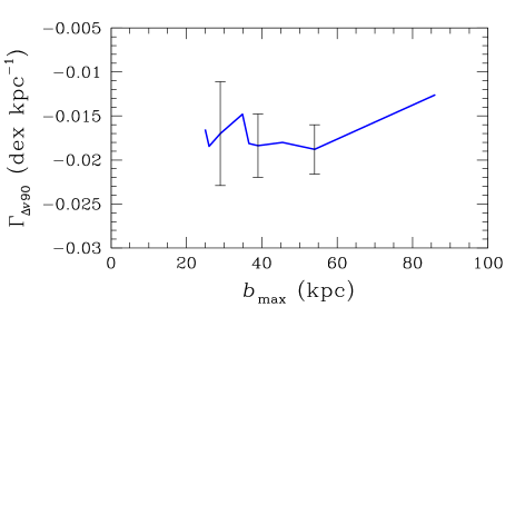
Figure 8: The gradient $\Gamma_{\Delta v90}$ of $\log(\mbox{$\Delta v_{90}$})$ measured from the centre of the DLA galaxy to $b_{\rm max}$ as a function of $b_{\rm max}$. It is seen that the gradient remains at a constant value of $\approx-0.017$ dex $\rm kpc^{-1}$out to $b\approx 60$ kpc. $1\sigma$ errors on $\Gamma_{\Delta v90}$ for three representative values of $b_{\rm max}$ are also shown.

4.2 Quantifying $\Gamma_{\Delta v90}$

There are two ways that we can attempt to determine $\Gamma_{\Delta v90}$. The first is to use the result from Arabsalmani et al. (2015) which says that there should be no dependence on $b$ in equation 6. In order to force the terms with $b$ to cancel, $1.46~{}\Gamma_{\Delta v90}$ must be equal to $-0.022$, i.e. $\Gamma_{\Delta v90}=-0.015$ as already shown in Sect. 3.1. This result is based on three independent data samples: (1) the GRB host sample providing [M/H], $\Delta v_{90}$ and $z_{\rm abs}$ to determine the redshift corrected relation, (2) the larger DLA sample providing [M/H], $\Delta v_{90}$ and $z_{\rm abs}$ for the comparison, and (3) the smaller DLA host sample providing $b$, ${\rm M}_{*}$, [M/H], $\Delta v_{90}$ and $z_{\rm abs}$ used to determine $\Gamma_{\rm[M/H]}$.

The other method is to measure $\Gamma_{\Delta v90}$ directly on the new data provided here, i.e. to fit a line to the data points of log($\Delta v_{90}$ / $\sigma_{\mathrm{e}m}$) vs. $b$ in Fig. 3 and determine its slope. The DLA galaxies in our sample have, by necessity, a large overlap with those of the Christensen et al. (2014) sample, but the use of direct measurements of $\sigma_{\mathrm{e}m}$ is new here. More importantly, while both the MZ and the $\Delta v_{90}$-[M/H] relations evolve with redshift, and therefore indirectly are linked to the choice of $\alpha_{0}$ and $ze(z)$, we here assume that $\sigma_{\mathrm{e}m}$ and $\Delta v_{90}$ are purely dictated by gravity and as such have no specific dependence on $z$ and therefore also no links to choices already made.

In Sect. 3.1 we already presented fits to the QSO-DLA data alone. Here we include the GRB-DLA data. We again discard GRB 090323A, but including it will not change the conclusions. We are then left with a total sample of 21 QSO-DLAs and 9 GRB-DLAs for which we again assign the median GRB impact parameter of 1.0 kpc to each. We use the method described in Møller et al. (2013) where we determine both the optimal $\chi^{2}$ fit and the natural (intrinsic) scatter ($\sigma_{\rm nat}$) simultaneously, and in order to test for a flattening of the slope we perform the fit from $b=0$ kpc out to $b=b_{\rm max}$ for values of $b_{\rm max}$ from 25 to 86 kpc. The result is shown in Fig. 8 and we see that out to $b_{\rm max}=54$ kpc there is no evidence for any flattening as $\Gamma_{\Delta v90}$ consistently displays a value of $\approx-0.017$ dex $\rm kpc^{-1}$. Only the object with the largest impact parameter at 86 kpc deviates from this trend, in agreement with the visual impression from Fig. 3. The $1\sigma$ error on the fit to 29 objects within $b_{\rm max}=54$ kpc is 0.0028 dex $\rm kpc^{-1}$ confirming the detection of the slope at $6\sigma$. The corresponding scatter is $\sigma_{\rm nat}=0.22$. The values of $\Gamma_{\Delta v90}$ from the two methods agree to within less than $1\sigma$.

4.3 Flattening of the gradients

From the models of DM halos, as well as the observations of extended flat rotation curves, it is expected that the steep CGM gradient we have found for $\log(\mbox{$\Delta v_{90}$})$ should flatten a larger radii. We show this in Fig. 3 as an example DM profile, and it is also there seen that the object with the largest $b$ does not follow the steep slope. It is slightly surprising that all the other points agree well with the same steep slope as far out as 54 kpc (as also shown in Fig. 8), but the sample is small with a significant scatter, so it is premature to speculate about implications of this yet.

The fact that GRB hosts follow QSO-DLAs is interesting though. This result is more significant since it is a single offset based on larger samples. What this means is that if the $\log(\mbox{$\Delta v_{90}$})$ gradient flattens at larger radii, then the metallicity would likely have to behave in a similar way to remain consistent. In this sense, the halo profile flattening would result in a prediction that there must be a corresponding flattening of the metallicity gradient.

4.4 Interpreting the $\Delta v_{90}$-[M/H] relation

Following the previous sections, and recalling the errors on the two gradients: $\Gamma_{\rm[M/H]}=-0.022\pm 0.001$ and $\Gamma_{\Delta v90}=-0.017\pm 0.003$ we can now formulate the final description of the $\Delta v_{90}$-[M/H] relation (equation 6) as

$${\rm[M/H]}=1.46\log(\mbox{$\Delta v_{90}$})+(0.003\pm 0.005)~{}b+\beta-ze(z)$$ (7)

where we see that after determining the two gradients independently, the dependence on impact parameter disappears to within the error. This means that the hope that some of the scatter in the relation was caused by a dependence on $b$, which could then be identified and removed (Møller et al., 2013), has been foiled. The scatter must have other causes. This conclusion is based on the assumption that the two gradients remain constant, or that they both flatten in a similar way. If only one of them flattens, or is truncated, there could still be a $b$ dependence in equation 6, even though this seems to be ruled out by the comparison to GRB hosts. An expansion of the current DLA galaxy samples at larger impact parameters would be required to answer this.

The main two takeaway points concerning the $\Delta v_{90}$-[M/H] relation is therefore that the main slope, $\alpha_{0}$, still represents the relation which exists for the centres of the galaxies, but that all the individual galaxies have been pushed down along this relation to a lower position, meaning that the metallicity follows the local value of $\Delta v_{90}$. The exact distance each galaxy has been pushed is a function of $b$. For DLA galaxies we find a median in our sample of $b_{\rm med}=11.8$ kpc, which means that on average a DLA galaxy in the mass range considered here will be lying on the underlying relation, but at a metallicity which is 0.26 dex lower than its central value. Because sub-DLAs usually have larger impact parameters they could have been shifted even further down the relation but if the gradients flatten at some $b$ then that would define the maximum shift.

The prediction above that the metallicity gradient does not add scatter to the $\Delta v_{90}$-[M/H] relation can be tested directly. In Appendix B we assemble an additional DLA galaxy sample for this test.

4.5 Quantifying $\beta$ and $ze(z)$

Equation 5 provides the general form of the $\Delta v_{90}$-[M/H] relation as a relation through the centre of galaxies but modified by their actual impact parameters. An observed relation reflects the same central relation but then modified by the sample average of random impact parameters which in general would cause a modified $\beta$ and possibly also a modified $ze(z)$. However, in Equation 7 we have showed that the combined effect of the impact parameter is to move galaxies along the central relation which means that the observed relation is identical to the central relation, but all galaxies are instead pushed to lower metallicities. $\beta$ and $ze(z)$ are therefore conserved within the redshift range considered here, and for consistency with $\alpha_{0}$ and $\Gamma_{\rm[M/H]}$ one must use the corresponding values $\beta=-3.33$ and $ze(z)=0.35~{}z$ (for $z<2.62$); $ze(z)=0.35\times 2.62$ (for $z>2.62$) (Møller et al., 2013).

4.6 A simple physical interpretation of the MZ relation

Let us try to view the “local history of the universe” from the point of view of local gravitational well depth. At a given gravitational potential contour, and summed over the history of the universe, a certain amount of pristine gas will have passed this contour on its way into the well, a certain amount of metals will have been produced by stars inside the contour and a certain amount of enriched gas will have been pushed back out through this contour by outflows. Together those three processes define the metallicity on the contour.

The new results presented in this paper show that the way those three processes (infall, star formation and outflow) set the local metallicity, is directly linked to the local potential irrespective of redshift (in the redshift range covered by our data). In other words, the classic MZ relation is a special projection which is relating the integrated stellar mass inside the potential well to the luminosity-weighted average metallicity of the galaxy. The underlying relation is directly between the local values of the potential and the metallicity.

5 Conclusions

Arabsalmani et al. (2015) put forward the following bold proposal concerning the root of the mass metallicity relation: “ … then this means that the general concept of an MZ relation plus metallicity gradients simply is a convoluted and roundabout way of describing a much simpler underlying relation between metallicity and gravitational well depth.”

In this paper we test this hypothesis. We carefully search the literature and data archives, and find that the required observational data for the test currently is at hand for 21 DLA/sub-DLA galaxies and 9 GRB host galaxies. The test predicts that out to at least the maximum range of impact parameters for DLA galaxies, typically taken to be 20-30 kpc, the velocity dispersion of the halo gas should decrease as an approximately linear relation with a slope of $-0.015$ dex kpc^-1. We show that the current sample fully follows this prediction out to impact parameters of 40-60 kpc. We further explore if there is any evidence that this slope is a function of redshift, stellar mass or H i column density. We also test if the “classic dynamical tracer”, the relative velocity between $z_{\rm abs}$ and $z_{\rm em}$ (in this paper named $v_{\rm rel}$), holds similar dynamical information as the absorption line velocity width, $\Delta v_{90}$. We find that this is not the case and argue that this can be used to constrain the nature of individual DLA absorbing clouds.

Concisely our main findings can be summarized as

• We confirm that the mass metallicity relation of DLA and GRB host galaxies is local in nature. In particular that the metallicity (at least out to 20-30 kpc but possibly further) directly traces the gravitational potential.

• We show that the “CGM halo potential” of DLA galaxies, which here is taken to mean the inner 40-60 kpc, to within the intrinsic scatter can be described well by a linear function with a slope of $\Gamma_{\Delta v90}=-0.017\pm 0.003$ dex kpc^-1.

• Our sample covers redshifts from $z=0.16$ to $z=3.15$, we see no change in the above results over this redshift range.

• Our sample covers galaxy stellar masses in the range $\log{\rm M}_{*}/{\rm M_{\odot}}=9.4-11.06$, we see no significant evidence for a change in the above results over this stellar mass range.

• We compare the dynamical tracers $\Delta v_{90}$ and $v_{\rm rel}$, and find that taken together they favour an interpretation that DLA absorption systems are composed of a series of independent systems distributed along the pencil beam through the halo, and disfavours a model of a single but complex cloud moving with a bulk velocity.

Based on the new results presented here it appears that the $\Delta v_{90}$-metallicity relation forms the underlying physical relation of which the well known MZ relation is a special projection, relating only the stellar mass fraction of the potential to the luminosity-weighted average metallicity of the galaxy.

6 Acknowledgements

It is a pleasure to thank Hadi Rahmani for kindly sharing HIRES and MUSE spectra. We are grateful to our referee who made several constructive suggestions. LC is supported by YDUN grant DFF 4090-00079. This is based on archival observations at ESO; Programme IDs: 074.A-0597(UVES), 078.A-0003(UVES), 078.A-0646(ADP), 278.A-5062(ADP), 080.A-0742(SINFONI), 087.A-0022(X-shooter) and 087.A-0414(X-shooter).

Appendix A Extraction of sample data

Below we provide details on individual absorbers and galaxies, including references to relevant data. In cases where we measured $\Delta v_{90}$ or $z_{\tau 50}$ on archival data (Q0021+0043, Q0153+0009, Q1439+1117, Q2233+1318, Q2328+0022 and Q2352-0028), we selected appropriate metal line transitions that are not saturated following the description in Ledoux et al. (2006). Where we correct $\Delta v_{90}$ values for resolution we use the method described by Arabsalmani et al. (2015).

Q0021+0043 = SDSS J002133.27+004300.9: Péroux et al. (2016) report $z_{\rm em}=0.94187$ from detection of H$\alpha$ emission at an impact parameter of $b=10.8$ arcsec, corresponding to 86 kpc in our assumed cosmology. They further report an emission line velocity dispersion of $\mbox{$\sigma_{\mathrm{e}m}$}=123\pm 11$ ${\rm km\,s^{-1}}$. Rao et al. (2011) report $z_{\rm abs}=0.9420$ and $\log N($H i$)=19.38_{-0.15}^{+0.10}$. We measured $\Delta v_{90}$ = 139 ${\rm km\,s^{-1}}$and $\mbox{$z_{\tau 50}$}=0.94181$ on the Si ii(1808) line using UVES ESO archive data (Programme-ID: 078.A-0003) (Péroux et al., 2016). We adopt $z_{\tau 50}$ as $z_{\rm abs}$ and find $v_{\rm rel}=-9\pm 5$ ${\rm km\,s^{-1}}$.

Q0151+045 = PHL 1226 = J015427.99+044818.2: Christensen et al. (2005) used IFU (PMAS) to identify the host of this sub-DLA. The host (named G4) as seen in continuum is 6.5” south and 1.5” west of the QSO, i.e. the angular distance of the galaxy continuum image is 6.7” and $b=18.5$ kpc. They also detected H$\alpha$ emission from G4 but with a centroid offset 1.4” to the south of the continuum image (their Fig. 5). They report $z_{\rm em}=0.1595\pm 0.0006$, but the line-emission appears to be kinematically coupled to only one side of G4 (their Fig.7) and they find it is offset to a lower redshift than the absorption by $v_{\rm rel}=+180$ ${\rm km\,s^{-1}}$. We have determined $\sigma_{\mathrm{e}m}$$=50\pm 20$ ${\rm km\,s^{-1}}$ (corrected for resolution) from the H$\alpha$ on the original data. Som et al. (2015) reported $\log N($H i)$=19.48\pm 0.10$, $z_{\rm abs}=0.1602$ and $\Delta v_{90}$$=152$ ${\rm km\,s^{-1}}$. Using SDSS photometry we have used standard SED fitting (see Fig. 9) and determined $\log{\rm M}_{*}/{\rm M_{\odot}}=9.73\pm 0.04$.

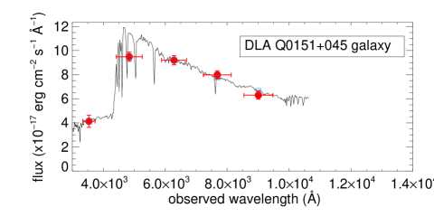
Figure 9: Spectral energy distribution fit from the HyperZ code (Bolzonella et al., 2000) for PHL 1226 resulting in a stellar mass of log M*$=9.73\pm 0.04$ derived from fitting the data points to galaxy templates using a Chabrier initial mass function.

Q0152-2001 = J015227.32–200107.0: using MUSE Rahmani et al. (2018) identified the host at $z_{\rm em}=0.78025\pm 0.00007$ of the $\log N($H i$)=19.1\pm 0.3$ absorber. They detect [O ii], [O iii] and H$\beta$ emission lines in the host at $b=54$ kpc, and from their HIRES spectrum they report $v_{\rm rel}=-78$ ${\rm km\,s^{-1}}$. They did not extract $\sigma_{\mathrm{e}m}$ and $\Delta v_{90}$, but they kindly provided us with a copy of both the reduced MUSE and HIRES data. We find $\mbox{$\sigma_{\mathrm{e}m}$}=104\pm 13$ ${\rm km\,s^{-1}}$(after correction for the spectral resolution of 2.6 Å) and $\mbox{$\Delta v_{90}$}=33$ ${\rm km\,s^{-1}}$.

0153+0009 = SDSS J015318.19+000911.4: Rhodin et al. (2018) report $z_{\rm em}=0.77085\pm 0.00003$, $\mbox{$\sigma_{\mathrm{e}m}$}=121\pm 8$ ${\rm km\,s^{-1}}$, $\log{\rm M}_{*}/{\rm M_{\odot}}=10.03^{+0.18}_{-0.08}$, and impact parameter $b=36.6$ kpc of a candidate counterpart of the $z=0.7714$, $\log N($H i$)=19.70\pm 0.09$ absorber (Rao et al., 2011). We measure $\mbox{$\Delta v_{90}$}=58$ ${\rm km\,s^{-1}}$ and $\mbox{$z_{\tau 50}$}=0.77219$ from UVES archive data (Adv. Data Products, Programme ID: 078.A-0646) using the Al iii1854 line (Péroux et al., 2008). We adopt $z_{\tau 50}$ as $z_{\rm abs}$ and find $v_{\rm rel}=+227\pm 5$ ${\rm km\,s^{-1}}$.

0302-223 = J030449.87–221151.9: Péroux et al. (2011b) determine $z_{\rm em}=1.00946$, $\mbox{$\sigma_{\mathrm{e}m}$}=59$ ${\rm km\,s^{-1}}$, $v_{\rm rel}=-1$ ${\rm km\,s^{-1}}$ and impact parameter $b=25$ kpc of the counterpart of a $\log N($H i$)=20.36\pm 0.11$ DLA at $z_{\rm abs}=1.00945$ (Pettini et al., 2000). They do not provide an error on $\sigma_{\mathrm{e}m}$. Looking at their high S/N data we estimate that 10% is a conservative upper limit, and we therefore use $\mbox{$\sigma_{\mathrm{e}m}$}=59\pm 6$. Møller et al. (2013) determine $\mbox{$\Delta v_{90}$}=61$ ${\rm km\,s^{-1}}$ and Christensen et al. (2014) $\log{\rm M}_{*}/{\rm M_{\odot}}=9.65\pm 0.08$.

0918+1636-1 = SDSS J091826.16+163609.0: for the $\log N($H i$)=21.26\pm 0.06$ DLA Fynbo et al. (2013) report the detection of $[$Oiii$]$ with FWHM = $50\pm 12$ ${\rm km\,s^{-1}}$(corrected for resolution and corresponding to $\mbox{$\sigma_{\mathrm{e}m}$}=21\pm 5$), at $z_{\rm em}=2.4128\pm 0.0002$ and at an impact parameter of $b<2$ kpc. They also report $v_{\rm rel}=-38\pm 25$ ${\rm km\,s^{-1}}$and $\mbox{$\Delta v_{90}$}=350\pm 2$ ${\rm km\,s^{-1}}$. Applying the correction for the X-shooter 45 ${\rm km\,s^{-1}}$ resolution provides an intrinsic $\mbox{$\Delta v_{90}$}=344$ ${\rm km\,s^{-1}}$.

0918+1636-2: for the DLA at $z_{\rm abs}=2.5832$ Fynbo et al. (2013) report $b=16.2\pm 0.2$ kpc, $\mbox{$\Delta v_{90}$}=295\pm 2$ ${\rm km\,s^{-1}}$ and $\log N($H i$)=20.96$. As above we apply the correction for resolution and get $\mbox{$\Delta v_{90}$}=288$ ${\rm km\,s^{-1}}$. Based on their detection of $[$Oiii$]$ in emission they find $z_{\rm em}=2.58277\pm 0.00010$, $v_{\rm rel}=+36\pm 20$ ${\rm km\,s^{-1}}$ and $\mathrm{FWHM=252\pm 23}$ ${\rm km\,s^{-1}}$ (corrected for resolution), i.e. $\mbox{$\sigma_{\mathrm{e}m}$}=107\pm 10$ ${\rm km\,s^{-1}}$. $\log{\rm M}_{*}/{\rm M_{\odot}}=10.33\pm 0.08$ was reported by Christensen et al. (2014).

1009-0026 = SDSS J100930.47–002619.1: Péroux et al. (2011b) determine the emission redshift $z_{\rm em}=0.8864$, and impact parameter $b=39$ kpc of the counterpart of a $\log N($H i$)=19.48^{+0.05}_{-0.06}$ absorber at $z_{\rm abs}=0.8866$, i.e. $v_{\rm rel}=+32$ ${\rm km\,s^{-1}}$. Based on their H$\alpha$ SINFONI data cube they describe a distribution of $\sigma_{\mathrm{e}m}$ peaking at 190 ${\rm km\,s^{-1}}$ in the centre but only 60-70 ${\rm km\,s^{-1}}$ in the outer parts. Since they do not provide an integrated value we downloaded the data from the ESO archive (programme-ID: 080.A-0742) and integrated the total H$\alpha$ line to obtain $\mbox{$\sigma_{\mathrm{e}m}$}=174\pm 5$ ${\rm km\,s^{-1}}$. Meiring et al. (2009b) determined $\mbox{$\Delta v_{90}$}=94$ ${\rm km\,s^{-1}}$, and Christensen et al. (2014) report $\log{\rm M}_{*}/{\rm M_{\odot}}=11.06\pm 0.03$.

J1135-0010 = SDSS J113520.39–001053.6: Noterdaeme et al. (2012) detect $[$Oiii$]$ and H$\alpha$ emission at an impact parameter of $b=0.8$ kpc (when converted to our cosmology) from this $\log N($H i$)=22.10\pm 0.05$, $z_{\rm abs}=2.2066$, DLA, but they provide only an approximate FWHM. We therefore use the ADS Dexter data extraction applet (Demleitner et al., 2001) to measure individual values of the three detected lines and combine them to obtain $\mbox{$\sigma_{\mathrm{e}m}$}=53\pm 3$ ${\rm km\,s^{-1}}$ (corrected for resolution). They do not provide separate $z_{\rm abs}$ and $z_{\rm em}$, but from their figure 3 we see that the individual transitions show a range of $v_{\rm rel}$ covering both positive and negative values. On average we find $v_{\rm rel}=-20\pm 10$ ${\rm km\,s^{-1}}$. Kulkarni et al. (2012) published high resolution spectroscopy but did not measure $\Delta v_{90}$ . We used ADS Dexter to extract $\mbox{$\Delta v_{90}$}=168$ ${\rm km\,s^{-1}}$ using the unsaturated Cr ii2056 line.

1228-1139/B1228-113 = J123055.56–113909.8: Neeleman et al. (2018) report the detection of line emission from CO and H$\alpha$ at an impact parameter of 3.5 arcsec, corresponding to $b=30$ kpc at $z_{\rm abs}=2.19289$. They further find $\log N($H i$)=20.60\pm 0.10$, $\mbox{$\Delta v_{90}$}=163\pm 10$ ${\rm km\,s^{-1}}$, $z_{\rm em}=2.1912$ (H$\alpha$). From this we find $v_{\rm rel}=+159\pm 18$ ${\rm km\,s^{-1}}$, and from the extracted SINFONI spectrum (programme-ID: 080.A-0742) we measure $\mbox{$\sigma_{\mathrm{e}m}$}=93\pm 31$ from H$\alpha$.

B1323-0021 = J132323.78–002155.3: Møller et al. (2018) report the detection of line emission from CO, H$\alpha$ and $[$Oii$]$ from a candidate DLA galaxy (Hewett & Wild, 2007) at an impact parameter of 1.25 arcsec (Chun et al., 2010). They further find $\log{\rm M}_{*}/{\rm M_{\odot}}=10.80^{+0.07}_{-0.14}$, $b=9.1$ kpc, $\log N($H i$)=20.4^{+0.3}_{-0.4}$, $z_{\rm em}=0.7171\pm 0.0001$, $z_{\rm abs}=\mbox{$z_{\tau 50}$}=0.71612$ ${\rm km\,s^{-1}}$, $v_{\rm rel}=-171\pm 18$, $\mbox{$\Delta v_{90}$}=141\pm 2$ ${\rm km\,s^{-1}}$ and $\mbox{$\sigma_{\mathrm{e}m}$}=101\pm 14$ ${\rm km\,s^{-1}}$(based on their FWHM of H$\alpha$).

1436-0051A = SDSS J143645.05–005150.6: Rhodin et al. (2018) determined $z_{\rm em}=0.73749\pm 0.00003$, $\mbox{$\sigma_{\mathrm{e}m}$}=99\pm 25$ ${\rm km\,s^{-1}}$, $\log{\rm M}_{*}/{\rm M_{\odot}}=10.41^{+0.09}_{-0.08}$, and $b=45.5$ kpc to confirm a candidate counterpart of the $z_{\rm abs}=0.7377$, $\log N($H i$)=20.08\pm 0.11$, $\mbox{$\Delta v_{90}$}=71$ ${\rm km\,s^{-1}}$ absorber (Meiring et al., 2009b).

1436-0051B Rhodin et al. (2018): determined the emission redshift $z_{\rm em}=0.92886\pm 0.00002$, $\mbox{$\sigma_{\mathrm{e}m}$}=33\pm 11$ ${\rm km\,s^{-1}}$, $\log{\rm M}_{*}/{\rm M_{\odot}}=10.20^{+0.11}_{-0.08}$, and impact parameter $b=34.9$ kpc of a candidate counterpart of the $z_{\rm abs}=0.9281$, $\log N($H i$)<18.8$, $\mbox{$\Delta v_{90}$}=62$ ${\rm km\,s^{-1}}$ absorber (Meiring et al., 2009b). Meiring et al. (2008) reported $\log N($Zn ii$)=12.29\pm 0.06$ and Straka et al. (2016) $\log N($H i$)=18.4\pm 0.98$. Without ionization correction this would provide a metallicity of $+1.26\pm 1.02$. Straka et al. (2016) computed ionization corrections and found a metallicity of $-0.05\pm 0.55$ implying that the computed ionization corrections are the range $-1.78$ to $-0.84$ dex or a factor of 60 to 7.

1439+1117 = SDSS J143912.04+111740.6: Rudie et al. (2017) report the detection of line emission at $z_{\rm em}=2.4189\pm 0.0001$ from a $\log{\rm M}_{*}/{\rm M_{\odot}}=10.74^{+0.18}_{-0.16}$ galaxy at impact 4.7 arcsec ($b=39$ kpc) from J1439+1117. They give $v_{\rm rel}$ as $-46$ ${\rm km\,s^{-1}}$ and $\mbox{$\sigma_{\mathrm{e}m}$}=303\pm 12$ ${\rm km\,s^{-1}}$. We downloaded the UVES archive data used by Srianand et al. (2008) (Adv. Data Products, programme ID: 278.A-5062) and measure $\mbox{$\Delta v_{90}$}=338$ ${\rm km\,s^{-1}}$ and $\mbox{$z_{\tau 50}$}=2.41802$, both using the Fe ii1608 line. Using now $z_{\tau 50}$ for $z_{\rm abs}$ we find $v_{\rm rel}=-77$ ${\rm km\,s^{-1}}$. Srianand et al. (2008) report $\log N($H i$)=20.10\pm 0.10$. Rudie et al. (2017) argue that the host of this absorber is AGN dominated, and that the absorber therefore likely is influenced by AGN outflow. We include it in our sample because this provides us with an opportunity to test if a strong outflow will cause absorption systems to diverge from standard kinematic behaviour or not.

LBQS 2206-1958 = J220852.07–194359.86: Weatherley et al. (2005) report $[$Oiii$]$ line emission from two interacting galaxies at $z_{\rm em}=1.9220(2)$ and $z_{\rm em}=1.91972(8)$, both associated to a DLA at $z_{\rm abs}=1.919991(2)$. The two galaxies have impact parameters of 0.98 and 1.24 arcsec respectively, corresponding to $b=8.4\pm 0.3$ and $b=10.6\pm 0.3$ kpc, and their line widths and velocity offsets are given as FWHM$=220\pm 50$ ${\rm km\,s^{-1}}$, FWHM$=180\pm 25$ ${\rm km\,s^{-1}}$, $v_{\rm rel}=-210\pm 20$ ${\rm km\,s^{-1}}$ and $v_{\rm rel}=+29\pm 9$ ${\rm km\,s^{-1}}$. Ledoux et al. (2006) report $\mbox{$\Delta v_{90}$}=136$ ${\rm km\,s^{-1}}$ and $\log N($H i$)=20.67\pm 0.05$. The two galaxies are members of what appears to be an active merger (Møller et al., 2002) and Christensen et al. (2014) used SED fitting to compute the total stellar mass of the entire group $\log{\rm M}_{*}/{\rm M_{\odot}}=9.45\pm 0.30$. Here we assign “ownership” of the merging group to the main galaxy (named N-14-1C) at $b=8.4\pm 0.3$ kpc and compute $\mbox{$\sigma_{\mathrm{e}m}$}=93\pm 21$ ${\rm km\,s^{-1}}$.

2222-0946 = SDSS J222256.11–094636.3: Krogager et al. (2013) report the FWHM (corrected for resolution) of 5 different emission lines at $z_{\rm em}=2.3537$ and at good S-to-N. We combine all 5 measurements using inverse variance weighting and find $\mbox{$\sigma_{\mathrm{e}m}$}=49.0\pm 1.6$ ${\rm km\,s^{-1}}$. Fynbo et al. (2010) report $\log N($H i$)=20.65\pm 0.05$ and $\mbox{$\Delta v_{90}$}=185$ ${\rm km\,s^{-1}}$ which after correction for resolution (45 ${\rm km\,s^{-1}}$) becomes 174 ${\rm km\,s^{-1}}$. Krogager et al. (2017) find $b=6.3\pm 0.3$ kpc and Christensen et al. (2014) find $\log{\rm M}_{*}/{\rm M_{\odot}}=9.62\pm 0.12$. $z_{\rm em}$ is embedded inside the rather wide span of absorption components. To obtain a velocity offset we estimate $z_{\tau 50}$ as follows. From Table 2 of Krogager et al. (2013) we find that for three of the six low ionization species listed the median is in the second component (at 11 ${\rm km\,s^{-1}}$) while for the other three it is in the third component (at 73 ${\rm km\,s^{-1}}$). We therefore assign the relative offset to be between the two at $v_{\rm rel}=+42\pm 30$ ${\rm km\,s^{-1}}$.

2233+1318 = J223619.20+132620.3: Weatherley et al. (2005) report $[$Oiii$]$ line emission at $z_{\rm em}=3.15137\pm 0.00006$ with $\mbox{$\sigma_{\mathrm{e}m}$}=23^{+8}_{-13}$ ${\rm km\,s^{-1}}$. They also compute the velocity offset between $z_{\rm em}$ and $z_{\rm abs}=3.14930(7)$ to be $-150$ ${\rm km\,s^{-1}}$. In their section 3.1 they point out that the location of the line emission precisely matches the position of an existing HST-STIS image, but not the position of an HST-NICMOS image which is offset by 2.1 kpc. Therefore, this is likely line emission from a single site of star formation in an otherwise quiescent galaxy and as such the emission line width is representative of the smaller UV dominated region rather than the general, and older, stellar population. From the STIS position we obtain $b=19.5$ kpc, using the NICMOS position we find $b=21.6$ kpc. Christensen et al. (2014) found $\log{\rm M}_{*}/{\rm M_{\odot}}=9.85\pm 0.14$. We downloaded ESO-X-shooter archival data (PI: Cooke, Programme-ID: 087.A-0022) and measured $\mbox{$\Delta v_{90}$}=236.9$ ${\rm km\,s^{-1}}$ using the Fe ii1608 line. Correction for X-shooter resolution provides an intrinsic $\mbox{$\Delta v_{90}$}=228$ ${\rm km\,s^{-1}}$. We also measured the HI column density ($\log N($H i$)=20.00\pm 0.10$) and performed multi-component Voigt profile fitting of Fe ii1608 and Si ii1260,1304,1526,1808 using the code VoigtFit described in Krogager (2018). Among the fitted lines only Si ii1260 appears to be saturated. We determined column densities $\log N($Fe ii$)=14.10\pm 0.15$ and $\log N($Si ii$)=14.54\pm 0.08$ resulting in metallicities of [FeII/H]$=-1.37\pm 0.18$ and [SiII/H]$=-0.97\pm 0.13$.

2243-6031 = J224709.10–601545.0: Bouché et al. (2013) detect several emission lines at $z_{\rm em}=2.3283\pm 0.0001$ and report $\mbox{$\sigma_{\mathrm{e}m}$}=158\pm 5$ for a DLA host at an impact parameter of 3.1 arcsec ($b=26$ kpc). Based on a deep VLT/UVES spectrum Lopez et al. (2002) had previously reported $\log N($H i$)=20.67\pm 0.02$ for this absorber and a low-ion spectral complex consisting of 14 individual components spanning 330 ${\rm km\,s^{-1}}$. From their fit to each component, and using the same method as described for 2222-0946 above, we find that $z_{\rm abs}$, again defined here as the median optical depth redshift $z_{\tau 50}$, is $2.3298\pm 0.0001$ leading to $v_{\rm rel}=+135\pm 12$ ${\rm km\,s^{-1}}$. Ledoux et al. (2006) find $\mbox{$\Delta v_{90}$}=173$ ${\rm km\,s^{-1}}$ while Rhodin (in preparation) report $\log{\rm M}_{*}/{\rm M_{\odot}}=10.1\pm 0.1$.

2328+0022 = SDSS J232820.37+002238.1: Rhodin et al. (2018) determined the emission redshift $z_{\rm em}=0.65194\pm 0.00006$, $\mbox{$\sigma_{\mathrm{e}m}$}=56\pm 24$ ${\rm km\,s^{-1}}$, $\log{\rm M}_{*}/{\rm M_{\odot}}=10.62\pm 0.35$, and impact parameter $b=11.9$ kpc of the candidate counterpart of a $z_{\rm abs}=0.6519$, $\log N($H i$)=20.32\pm 0.06$ DLA (Rao et al., 2011). We measure $\mbox{$\Delta v_{90}$}=92$ ${\rm km\,s^{-1}}$ and $\mbox{$z_{\tau 50}$}=0.65179$ using the Mg i2852 line obtained from UVES archive data (programme ID: 074.A-0597). This results in $v_{\rm rel}=-27\pm 11$ ${\rm km\,s^{-1}}$.

2352-0028 = SDSS J235253.51−002850.4: Péroux et al. (2013) report detection of H$\alpha$ from the host of the sub-DLA with $\log N($H i$)=19.81^{+0.14}_{-0.11}$ at $z_{\rm abs}=1.0318$ (Rao et al., 2006). We downloaded the raw Sinfoni archive data (programme ID: 085.A-0708(A)) and measured a velocity dispersion of $125\pm 6$ km s^-1 by fitting the integrated H$\alpha$ emission line of the DLA galaxy, and correcting for instrumental resolution. Péroux et al. (2013) also provide (in their Fig. 10) a direct overlay of emission redshift on the low ion absorption profiles from which we estimate that $z_{\tau 50}$ is $40\pm 5$ ${\rm km\,s^{-1}}$ higher than $z_{\rm em}$, i.e. $v_{\rm rel}=+40\pm 5$ ${\rm km\,s^{-1}}$. Meiring et al. (2009b) report $\mbox{$\Delta v_{90}$}=164$ ${\rm km\,s^{-1}}$, and Augustin et al. (2018) find $\log{\rm M}_{*}/{\rm M_{\odot}}=9.4\pm 0.3$ and an impact parameter of 1.50 arcsec corresponding to $b=12.2$ kpc. We measure $\mbox{$z_{\tau 50}$}=1.03197$ from X-shooter archive data (programme ID 087.A-0414) using the Fe ii2374 line.

2358+0149 = SDSS J235854.4+014955.5: Srianand et al. (2016) detected $[$Oiii$]$ emission at an impact parameter of $1.5\pm 0.1$ arcsec with an intrinsic FWHM of 110 ${\rm km\,s^{-1}}$ corresponding to $\sigma_{\mathrm{e}m}$ = 46.7 ${\rm km\,s^{-1}}$. They provide no error on the emission line width, but from the figures we estimate an upper limit on the error of 20% and assign conservatively an error of 9 ${\rm km\,s^{-1}}$. They report $z_{\rm abs}$ and $z_{\rm em}$ of 2.97919 and 2.9784 respectively resulting in a velocity difference of $+60$ ${\rm km\,s^{-1}}$. In our cosmology the impact parameter corresponds to $b=11.8\pm 0.8$ kpc. They also provide $\Delta v_{90}$ values for an Fe ii line and Si ii1808. The Fe ii line is saturated so cannot be used, for the Si ii1808 line they give 141 ${\rm km\,s^{-1}}$ which (after correction for resolution) provides an intrinsic value of 135 km/s. They find $\log N($H i$)=21.69\pm 0.10$.

Appendix B Metallicity gradient and scatter of the $\Delta v_{90}$-[M/H] relation

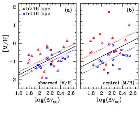
Figure 10: Standard $\Delta v_{90}$-[M/H] relation plots of the combined sample listed in Tables LABEL:tab:sample and LABEL:tab:Xsample. The colour/symbol coding divides the sample into small and large impact parameter. (a): observed metallicities only corrected for redshift evolution. (b): metallicities computed for the centres of the galaxies assuming a constant metallicity gradient independent of impact parameter. As predicted there is a larger scatter in (b).

In Sect. 3.1 and again in Sect. 4.2 we prove, using two different methods, that the $\Delta v_{90}$ radial gradient exactly cancels the effect of the metallicity gradient in the inner part of galaxy halos. From this, and from equation 7, we then assert in Sect. 4.4 that it must follow that the metallicity gradient in the inner part of the CGM cannot significantly contribute to the scatter of the $\Delta v_{90}$-[M/H] relation. Here we test this assertion. The test requires knowledge of the absorption metallicity of each galaxy, which is only the case for 19 of the galaxies in our original sample. However, the test does not require knowledge of $\sigma_{\mathrm{e}m}$ which makes it possible to expand our statistical sample for this test by including DLA/sub-DLA galaxies for which $\sigma_{\mathrm{e}m}$ is not known. The relevant data for this additional sample are listed in Table LABEL:tab:Xsample where we again have recomputed metallicities using Asplund et al. (2009) and the choices of De Cia et al. (2016) (their Table 1).

Table 2: Additional literature sample of DLA/sub-DLA galaxies for which impact parameter, $\Delta v_{90}$ and absorption metallicity is known, but where $\sigma_{\mathrm{e}m}$ is not known.

ID	$z_{\rm abs}$	$\log N($H i)	[M/H]	Tracer	$b$	$\Delta v_{90}$	References
					kpc	${\rm km\,s^{-1}}$
PKS 0439-433	0.1012	$19.63\pm 0.15$	$+0.08\pm 0.15$	S	7.6	275	1,   1,   1,   2,   1
1127-145	0.3127	$21.71\pm 0.08$	$-0.76\pm 0.10$	Zn	17.5	123	3,   3,   4,   5,   4
0827+243	0.5247	$20.30\pm 0.04$	$-0.54\pm 0.05$	Fe+0.4	38.4	188	4,   4,   4,   5,   4
0218-0831	0.5899	$20.84\pm 0.12$	$-0.26\pm 0.15$	Zn	14.7	261	6,   6,   6,   6,   6
1138+0139	0.6130	$21.25\pm 0.10$	$-0.65\pm 0.11$	Zn	12.2	105	6,   6,   6,   6,   6
0958+0549	0.6557	$20.54\pm 0.15$	$-1.21\pm 0.18$	Zn	20.3	112	6,   6,   6,   6,   6
2335+1501	0.67972	$19.70\pm 0.30$	$+0.07\pm 0.34$	Zn	27.0	103.5	7,   7,   7,   8,   9
0452-1640	1.0072	$20.98\pm 0.07$	$-0.99\pm 0.08$	Zn	16.2	70	10, 10, 10, 11,   9
Q1313+1441	1.7941	$21.30\pm 0.10$	$-0.86\pm 0.14$	Zn	11.2	164	12, 12, 12, 12, 12
2239-2949	1.82516	$19.84\pm 0.14$	$-0.67\pm 0.15$	Si	20.6	64	13, 13, 13, 13, 13
PKS0458-02	2.0396	$21.65\pm 0.09$	$-1.15\pm 0.10$	Zn	2.7	84	14, 14, 14, 12, 14
0338-0005	2.229	$21.12\pm 0.05$	$-1.37\pm 0.06$	Si	4.12	221	12, 12, 12, 12, 12
0124+0044	2.261	$20.70\pm 0.15$	$-0.67\pm 0.16$	Zn	10.9	142	15, 15, 15, 16, 15
Q2348-11	2.4263	$20.53\pm 0.06$	$-0.43\pm 0.08$	Zn	5.8	240	12, 12, 12, 12, 12
0139-0824	2.6773	$20.70\pm 0.15$	$-1.24\pm 0.20$	Si	13.0	100	16, 16, 17, 17, 16
0528-250	2.8110	$21.35\pm 0.07$	$-0.87\pm 0.07$	Zn	9.14	304	18, 18, 18, 19, 18

In Fig. 10(a) vi plot the standard $\Delta v_{90}$-[M/H] relation for this sample, corrected for redshift evolution by shifting all metallicities to $z=2.6$ as described in Møller et al. (2013). The sample contains 35 objects with a median impact parameter of 16 kpc. Objects with $b>16$ kpc are shown as red triangles, objects with smaller $b$ are marked as blue squares. In Fig. 10(b) we plot the same objects but here we show instead the central metallicities as computed from the impact parameters and assuming a constant metallicity gradient throughout. It is easy to see that this process in fact has increased the scatter rather than reduced it. To quantify this we have computed the usual linear relations to both the red and blue sub-samples (dotted lines) as well as to the total sample (full black line) in both figures B1(a) and B1(b). We use the fitting method from Møller et al. (2013) which computes zero point and intrisic scatter for a slope of 1.46 (see Sect. 4.1). The zero point offset between the red and blue sub-samples grows from 0.32 dex to 0.82 dex and the intrinsic scatter of the fit to the full sample grows from 0.46 dex to 0.72 dex when the central metallicities are used. This confirms the prediction that “correcting” for only the effect of metallicity gradient does not reduce the scatter of the relation as one would expect if $\Delta v_{90}$ did not depend on impact parameter.

References

- Arabsalmani et al. (2015) Arabsalmani, M., Møller, P., Fynbo, J. P. U., Christensen, L., Freudling, W., Savaglio, S., & Zafar, T., 2015, MNRAS, 446, 990
- Arabsalmani et al. (2018) Arabsalmani, M., Møller, P., Perley, D. A., et al., 2018, MNRAS, 473, 3312
- Asplund et al. (2009) Asplund, M., Grevesse, N., Sauval, A. J., & Scott, P., 2009, ARA&A, 47, 481
- Augustin et al. (2018) Augustin, R., Péroux, C., Møller, P., et al., 2018, MNRAS, 478, 3120
- Battaglia et al. (2005) Battaglia, G., Helmi, A., Morrison, H., et al., 2005, MNRAS, 364, 433
- Belfiore et al. (2017) Belfiore, F., Maiolino, R., Tremonti, C., et al., 2017, MNRAS, 469, 151
- Berg et al. (2015) Berg, T. A. M., Ellison, S. L., Prochaska, J. X., Venn, K. A., & Dessauges-Zavadsky, M., 2015, MNRAS, 452, 4326
- Berg et al. (2016) Berg, T. A. M., Ellison, S. L., Sánchez-Ramírez, R., et al., 2016, MNRAS, 463, 3021
- Bird et al. (2015) Bird, S., Haehnelt, M., Neeleman, M., Genel, S., Vogelsberger, M., & Hernquist, L., 2015, MNRAS, 447, 1834
- Bolzonella et al. (2000) Bolzonella, M., Miralles, J.-M., & Pelló, R., 2000, A&A, 363, 476
- Bouché et al. (2013) Bouché, N., Murphy, M. T., Kacprzak, G. G., Péroux, C., Contini, T., Martin, C. L., & Dessauges-Zavadsky, M., 2013, Science, 341, 50
- Chen et al. (2005) Chen, H.-W., Kennicutt, Jr., R. C., & Rauch, M., 2005, ApJ, 620, 703
- Christensen & Hjorth (2017) Christensen, L. & Hjorth, J., 2017, MNRAS, 470, 2599
- Christensen et al. (2014) Christensen, L., Møller, P., Fynbo, J. P. U., & Zafar, T., 2014, MNRAS, 445, 225
- Christensen et al. (2019) Christensen, L., Møller, P., Rhodin, N. H. P., Heintz, K. E., & Fynbo, J. P. U., 2019, submitted
- Christensen et al. (2005) Christensen, L., Schulte-Ladbeck, R. E., Sánchez, S. F., Becker, T., Jahnke, K., Kelz, A., Roth, M. M., & Wisotzki, L., 2005, A&A, 429, 477
- Christensen et al. (2007) Christensen, L., Wisotzki, L., Roth, M. M., Sánchez, S. F., Kelz, A., & Jahnke, K., 2007, A&A, 468, 587
- Chun et al. (2010) Chun, M. R., Kulkarni, V. P., Gharanfoli, S., & Takamiya, M., 2010, AJ, 139, 296
- De Cia et al. (2016) De Cia, A., Ledoux, C., Mattsson, L., Petitjean, P., Srianand, R., Gavignaud, I., & Jenkins, E. B., 2016, A&A, 596, A97
- Dehnen (1993) Dehnen, W., 1993, MNRAS, 265, 250
- Demleitner et al. (2001) Demleitner, M., Accomazzi, A., Eichhorn, G., Grant, C. S., Kurtz, M. J., & Murray, S. S., 2001, Astronomical Society of the Pacific Conference Series, 238, 321
- Fynbo et al. (2013) Fynbo, J. P. U., Geier, S. J., Christensen, L., et al., 2013, MNRAS, 436, 361
- Fynbo et al. (2010) Fynbo, J. P. U., Laursen, P., Ledoux, C., et al., 2010, MNRAS, 408, 2128
- Fynbo et al. (2011) Fynbo, J. P. U., Ledoux, C., Noterdaeme, P., et al., 2011, MNRAS, 413, 2481
- Hernquist (1990) Hernquist, L., 1990, ApJ, 356, 359
- Hewett & Wild (2007) Hewett, P. C. & Wild, V., 2007, MNRAS, 379, 738
- Jaffe (1983) Jaffe, W., 1983, MNRAS, 202, 995
- Kanekar et al. (2014) Kanekar, N., Prochaska, J. X., Smette, A., et al., 2014, MNRAS, 438, 2131
- Klitsch et al. (2018) Klitsch, A., Péroux, C., Zwaan, M. A., Smail, I., Oteo, I., Biggs, A. D., Popping, G., & Swinbank, A. M., 2018, MNRAS, 475, 492
- Komatsu et al. (2011) Komatsu, E., Smith, K. M., Dunkley, J., et al., 2011, ApJS, 192, 18
- Krogager (2018) Krogager, J.-K., 2018, VoigtFit: Absorption line fitting for Voigt profiles. Astrophysics Source Code Library
- Krogager et al. (2013) Krogager, J.-K., Fynbo, J. P. U., Ledoux, C., et al., 2013, MNRAS, 433, 3091
- Krogager et al. (2017) Krogager, J.-K., Møller, P., Fynbo, J. P. U., & Noterdaeme, P., 2017, MNRAS, 469, 2959
- Kulkarni et al. (2012) Kulkarni, V. P., Meiring, J., Som, D., Péroux, C., York, D. G., Khare, P., & Lauroesch, J. T., 2012, ApJ, 749, 176
- Lane et al. (1998) Lane, W., Smette, A., Briggs, F., Rao, S., Turnshek, D., & Meylan, G., 1998, AJ, 116, 26
- Le Brun et al. (1997) Le Brun, V., Bergeron, J., Boisse, P., & Deharveng, J. M., 1997, A&A, 321, 733
- Ledoux et al. (2006) Ledoux, C., Petitjean, P., Fynbo, J. P. U., Møller, P., & Srianand, R., 2006, A&A, 457, 71
- Lopez et al. (2002) Lopez, S., Reimers, D., D’Odorico, S., & Prochaska, J. X., 2002, A&A, 385, 778
- Lyman et al. (2017) Lyman, J. D., Levan, A. J., Tanvir, N. R., et al., 2017, MNRAS, 467, 1795
- Maiolino et al. (2008) Maiolino, R., Nagao, T., Grazian, A., et al., 2008, A&A, 488, 463
- Meiring et al. (2009a) Meiring, J. D., Kulkarni, V. P., Lauroesch, J. T., Péroux, C., Khare, P., & York, D. G., 2009a, MNRAS, 393, 1513
- Meiring et al. (2008) Meiring, J. D., Kulkarni, V. P., Lauroesch, J. T., Péroux, C., Khare, P., York, D. G., & Crotts, A. P. S., 2008, MNRAS, 384, 1015
- Meiring et al. (2009b) Meiring, J. D., Lauroesch, J. T., Kulkarni, V. P., Péroux, C., Khare, P., & York, D. G., 2009b, MNRAS, 397, 2037
- Meiring et al. (2007) Meiring, J. D., Lauroesch, J. T., Kulkarni, V. P., Péroux, C., Khare, P., York, D. G., & Crotts, A. P. S., 2007, MNRAS, 376, 557
- Møller et al. (2018) Møller, P., Christensen, L., Zwaan, M. A., et al., 2018, MNRAS, 474, 4039
- Møller et al. (2004) Møller, P., Fynbo, J. P. U., & Fall, S. M., 2004, A&A, 422, L33
- Møller et al. (2013) Møller, P., Fynbo, J. P. U., Ledoux, C., & Nilsson, K. K., 2013, MNRAS, 430, 2680
- Møller & Warren (1993) Møller, P. & Warren, S. J., 1993, A&A, 270, 43
- Møller et al. (2002) Møller, P., Warren, S. J., Fall, S. M., Fynbo, J. U., & Jakobsen, P., 2002, ApJ, 574, 51
- Moran et al. (2012) Moran, S. M., Heckman, T. M., Kauffmann, G., et al., 2012, ApJ, 745, 66
- Neeleman et al. (2018) Neeleman, M., Kanekar, N., Prochaska, J. X., Christensen, L., Dessauges-Zavadsky, M., Fynbo, J. P. U., Møller, P., & Zwaan, M. A., 2018, ApJ, 856, L12
- Neeleman et al. (2016) Neeleman, M., Prochaska, J. X., Zwaan, M. A., et al., 2016, ApJ, 820, L39
- Neeleman et al. (2013) Neeleman, M., Wolfe, A. M., Prochaska, J. X., & Rafelski, M., 2013, ApJ, 769, 54
- Noterdaeme et al. (2012) Noterdaeme, P., Laursen, P., Petitjean, P., et al., 2012, A&A, 540, 63
- Noterdaeme et al. (2008) Noterdaeme, P., Petitjean, P., Ledoux, C., Srianand, R., & Ivanchik, A., 2008, A&A, 491, 397
- Péroux et al. (2013) Péroux, C., Bouché, N., Kulkarni, V. P., & York, D. G., 2013, MNRAS, 436, 2650
- Péroux et al. (2011a) Péroux, C., Bouché, N., Kulkarni, V. P., York, D. G., & Vladilo, G., 2011a, MNRAS, 410, 2237
- Péroux et al. (2011b) —, 2011b, MNRAS, 410, 2251
- Péroux et al. (2008) Péroux, C., Meiring, J. D., Kulkarni, V. P., Khare, P., Lauroesch, J. T., Vladilo, G., & York, D. G., 2008, MNRAS, 386, 2209
- Péroux et al. (2016) Péroux, C., Quiret, S., Rahmani, H., et al., 2016, MNRAS, 457, 903
- Pettini et al. (2000) Pettini, M., Ellison, S. L., Steidel, C. C., Shapley, A. E., & Bowen, D. V., 2000, ApJ, 532, 65
- Prochaska & Wolfe (1997) Prochaska, J. X. & Wolfe, A. M., 1997, ApJ, 487, 73
- Rahmani et al. (2018) Rahmani, H., Péroux, C., Schroetter, I., et al., 2018, MNRAS, 480, 5046
- Rahmani et al. (2016) Rahmani, H., Péroux, C., Turnshek, D. A., et al., 2016, MNRAS, 463, 980
- Rao et al. (2011) Rao, S. M., Belfort-Mihalyi, M., Turnshek, D. A., Monier, E. M., Nestor, D. B., & Quider, A., 2011, MNRAS, 416, 1215
- Rao et al. (2006) Rao, S. M., Turnshek, D. A., & Nestor, D. B., 2006, ApJ, 636, 610
- Rhodin et al. (2018) Rhodin, N. H. P., Christensen, L., Møller, P., Zafar, T., & Fynbo, J. P. U., 2018, ArXiv e-prints
- Rudie et al. (2017) Rudie, G. C., Newman, A. B., & Murphy, M. T., 2017, ApJ, 843, 98
- Sánchez et al. (2014) Sánchez, S. F., Rosales-Ortega, F. F., Iglesias-Páramo, J., et al., 2014, A&A, 563, A49
- Sánchez et al. (2013) Sánchez, S. F., Rosales-Ortega, F. F., Jungwiert, B., et al., 2013, A&A, 554, A58
- Sánchez-Menguiano et al. (2018) Sánchez-Menguiano, L., Sánchez, S. F., Pérez, I., et al., 2018, A&A, 609, A119
- Savaglio et al. (2012) Savaglio, S., Rau, A., Greiner, J., et al., 2012, MNRAS, 420, 627
- Som et al. (2015) Som, D., Kulkarni, V. P., Meiring, J., York, D. G., Péroux, C., Lauroesch, J. T., Aller, M. C., & Khare, P., 2015, ApJ, 806, 25
- Srianand et al. (2016) Srianand, R., Hussain, T., Noterdaeme, P., Petitjean, P., Krühler, T., Japelj, J., Pâris, I., & Kashikawa, N., 2016, MNRAS, 460, 634
- Srianand et al. (2008) Srianand, R., Noterdaeme, P., Ledoux, C., & Petitjean, P., 2008, A&A, 482, L39
- Steidel et al. (1995) Steidel, C. C., Pettini, M., & Hamilton, D., 1995, AJ, 110, 2519
- Straka et al. (2016) Straka, L. A., Johnson, S., York, D. G., Bowen, D. V., Florian, M., Kulkarni, V. P., Lundgren, B., & Péroux, C., 2016, MNRAS, 458, 3760
- Tremonti et al. (2004) Tremonti, C. A., Heckman, T. M., Kauffmann, G., et al., 2004, ApJ, 613, 898
- Warren & Møller (1996) Warren, S. J. & Møller, P., 1996, A&A, 311, 25
- Warren et al. (2001) Warren, S. J., Møller, P., Fall, S. M., & Jakobsen, P., 2001, MNRAS, 326, 759
- Weatherley et al. (2005) Weatherley, S. J., Warren, S. J., Møller, P., Fall, S. M., Fynbo, J. U., & Croom, S. M., 2005, MNRAS, 358, 985
- Wolfe & Prochaska (1998) Wolfe, A. M. & Prochaska, J. X., 1998, ApJ, 494, L15
- Wolfe et al. (2008) Wolfe, A. M., Prochaska, J. X., Jorgenson, R. A., & Rafelski, M., 2008, ApJ, 681, 881
- Wuyts et al. (2016) Wuyts, E., Wisnioski, E., Fossati, M., et al., 2016, ApJ, 827, 74
- Zafar et al. (2017) Zafar, T., Møller, P., Péroux, C., Quiret, S., Fynbo, J. P. U., Ledoux, C., & Deharveng, J.-M., 2017, MNRAS, 465, 1613