Superfast amplification and superfast nonlinear saturation of perturbations as the mechanism of turbulence

Abstract

Ruelle predicted that the maximal amplification of perturbations in homogeneous isotropic turbulence is exponential $e^{\sigma\sqrt{Re}t}$ (where $\sigma\sqrt{Re}$ is the maximal Liapunov exponent). In our earlier works, we predicted that the maximal amplification of perturbations in fully developed turbulence is faster than exponential $e^{\sigma\sqrt{Re}\sqrt{t}+\sigma_{1}t}$. That is, we predicted superfast initial amplification of perturbations. Built upon our earlier numerical verification of our prediction, here we conduct a large numerical verification with resolution up to $2048^{3}$ and Reynolds number up to $6210$. Our direct numerical simulation here confirms our analytical prediction. Our numerical simulation also demonstrates that such superfast amplification of perturbations leads to superfast nonlinear saturation. We conclude that such superfast amplification and superfast nonlinear saturation of ever existing perturbations serve as the mechanism for the generation, development and persistence of fully developed turbulence.

Turbulence is ubiquitous in nature, and most of air and water flows are turbulent. Unfortunately such a common problem is the most important unsolved problem of classical physics according to Richard Feyman. From weather forecasting in meterology to airplane flight, turbulence poses the major scientific challenge. Turbulence as an open problem has two aspects: turbulence engineering and turbulence physics Li13 . Turbulence engineering deals with how to describe turbulence in engineering, and turbulence physics deals with the physical mechanism of turbulence. In pursuit of the understanding of turbulence physics, the classical hydrodynamic instability theory was developed Li18 . The scope of hydrodynamic instability thery is very limited, and the limited result is far from satisfactory in answering the basic question of transition from laminar flow to turbulence. With the development of chaos theory, the idea of chaos was introduced for undertanding turbulence RT71 . On the other hand, there are fundamental differences between chaos and turbulence according to experimental experts on turbulence.

Ever since Ruelle and Takens introduced the idea of chaos for understanding the mechanism of turbulence RT71 , there has been constant effort in validating the idea BJPV05 . At moderate Reynolds number, some features of chaos are indeed embedded in transient turbulence KK01 -LK15 . A key measure of chaos is the Liapunov exponent. Ruelle predicted that the maximal Liapunov exponent in homogeneous isotropic turbulence is proportional to the square root of the Reynolds number $\sigma\sqrt{Re}$ Rue79 -BH18 . Extensive numerical studies on Ruelle’s prediction have been conducted over the years CJVP93 -BH18 . Ruelle’s prediction is based on the assumption that the maximal Liapunov exponent is the inverse of the Kolmogorov time scale which makes numerical resolution a challenging problem. On the other hand, experimental experts on turbulence do not believe that fully developed turbulence behaves as low-dimensional chaos. Fully developed turbulence is more violent than chaos. Chaos is often in the form of a strange attractor which is characterized by exponential amplifications of perturbations within the attractor, with the coefficient of the exponent being the so-called Liapunov exponent. We predicted that the maximal amplification of perturbations in fully developed turbulence is faster than exponential Li14 -Li18 ,

$$e^{\sigma\sqrt{Re}\sqrt{t}+\sigma_{1}t},$$ (1)

where $\sigma$ and $\sigma_{1}$ are two positive constants, $\sigma_{1}=\sqrt{\frac{e}{2}}\sigma$. When the time $t$ is small, $\sqrt{t}$ is much bigger than $t$. Thus we predicted that initial stage maximal amplification of perturbations is superfast (much faster than exponential). Together with the large Reynolds number in the fully developed turbulence regime, such superfast amplification of perturbations will quickly reach nonlinear saturation during which time the second exponent term $\sigma_{1}t$ (corresponding to a exponential factor) is much smaller than the first term $\sigma\sqrt{Re}\sqrt{t}$. Ruelle’s prediction is based on dimension analysis of the Kolmogorov time scale Rue79 . Our prediction is based on rigorous analysis on the Navier-Stokes equations Li14 -IL18 . We have conducted an extensive low resolution numerical verification on our prediction FL18 . Our low resolution numerical simulations were not able to get into fully developed turbulence regime. On the other hand, the numerical investigation showed that our analytical prediction applies to a wide regime beyond fully developed turbulence. Built upon our earlier numerical verification FL18 , here we conduct a large numerical verification with resolution up to $2048^{3}$ and Reynolds number up to $6210$. We carry out direct numerical simulations on the three dimensional Navier-Stokes equations in the homogeneous isotropic turbulence regime. It is in such a fully developed homogeneous isotropic turbulence regime that our analytical prediction is most likely to be accurate. Our numerical results here indeed confirm our analytical prediction. Our numerical simulation also demonstrates that such superfast amplification of perturbations leads to superfast nonlinear saturation. We conclude that such superfast amplification and superfast nonlinear saturation of ever existing perturbations serve as the mechanism for the generation, development and persistence of fully developed turbulence.

Unlike the Lagrangian approach which tracks the trajectories of individual fluid particles, here we use the Eulerian approach which tracks the evolution of the entire fluid field starting from an initial condition of the fluid field. We will add a perturbation to the initial condition and track the evolution of the perturbation either nonlinearly or linearly. By subtracting the two fluid fields, we are tracking the evolution of the perturbation nonlinearly. By subtracting the Navier-Stokes equations along the two fluid fields, we get the governing equations of the nonlinear evolution of the perturbation. By dropping the nonlinear terms of the perturbation, we get the governing equations of the linear evolution of the perturbation, and by solving which we track the evolution of the perturbation linearly.

We conduct direct numerical simulations on the three dimensional Navier-Stokes equations under periodic boundary condition of period $(2\pi)^{3}$ with a de-aliased pseudo-spectral code Yof12

$$\partial_{t}{\bf u}+{\bf u}\cdot\nabla{\bf u}=-\nabla p+\nu\Delta{\bf u}+{\bf f},\ \nabla\cdot{\bf u}=0,$$ (2)

where ${\bf u}$ is the velocity field, $p$ is the pressure, $\nu$ is the viscosity, and ${\bf f}$ is the external forcing. The external forcing will only force low wave numbers (large scales), and the Fourier transform $\tilde{{\bf f}}$ of ${\bf f}$ is given by Mac97

$$\tilde{{\bf f}}({\bf k},t)=\left\{\begin{array}[]{l}\frac{\epsilon_{f}}{2E_{f}}\tilde{{\bf u}}({\bf k},t),\ \text{if }0<|{\bf k}|<k_{f},\cr 0,\quad\text{otherwise},\cr\end{array}\right.$$ (3)

where $\tilde{{\bf u}}({\bf k},t)$ is the Fourier transform of the velocity field ${\bf u}$, $E_{f}$ is the kinetic energy restricted to the forcing band, $E_{f}=\frac{1}{2}\sum_{0<|{\bf k}|<k_{f}}|\tilde{{\bf u}}({\bf k},t)|^{2}$, and one can view the external forcing as an energy pumping through the low wave numbers with the energy pumping rate $\epsilon_{f}$, from the following energy equation

$$\frac{d}{dt}\sum_{{\bf k}}|\tilde{{\bf u}}|^{2}=-\nu\sum_{{\bf k}}|{\bf k}\tilde{{\bf u}}|^{2}+\epsilon_{f},$$ (4)

here the first term on the right hand side is the turbulence energy dissipation rate. Through such energy pumping that balances the energy dissipation, one can drive the turbulence into a statistically steady state of homogeneous isotropic turbulence. The external forcing here has been well tested by other researchers KI06 LM15 . For our numerical simulations here, we choose $k_{f}=2.5$ and $\epsilon_{f}=0.1$. The Reynolds number is specifically defined by $Re=\frac{VL}{\nu}$, where $V$ is the rms velocity, and $L$ is the integral length scale $L=\frac{3\pi}{8E}\sum_{{\bf k}}\frac{|\tilde{{\bf u}}({\bf k})|^{2}}{|{\bf k}|}$, where $E$ is the kinetic energy. The large eddy turnover time is given by $T_{0}=L/V$. In our simulations, the large eddy turnover time is around $2$. All our direct numerical simulations are well resolved to scales smaller than the Kolmogorov scale. We also test resolution to scales much smaller than the Kolmogorov scale to make sure our resolution is statistically sufficient.

After we run our direct numerical simulation to a statistically steady state of homogeneous isotropic turbulence, we introduce a perturbation by first making a copy of the velocity field at a time step and then not calling the external forcing at that time step for one copy of the velocity field. Thus the perturbation will be in the band of wave numbers of the external forcing (3), $0<|{\bf k}|<k_{f}$. After that time step, both fields will call the external forcing normally. We can then track the nonlinear or linear evolution of the perturbation as described before. We denote the nonlinear evolution of the perturbation by $\Delta{\bf u}({\bf x},t)$, the linear evolution of the perturbation by $\delta{\bf u}({\bf x},t)$, and their energy norms by $\Delta(t)=\Delta u(t)$ and $\delta u(t)$:

$$\Delta(t)=\Delta u(t)=\left(\sum_{{\bf k}}|\widetilde{\Delta{\bf u}}({\bf k},t)|^{2}\right)^{1/2},$$ (5)

$$\delta u(t)=\left(\sum_{{\bf k}}|\widetilde{\delta{\bf u}}({\bf k},t)|^{2}\right)^{1/2}.$$ (6)

We notice that the nonlinear amplification $\Delta u(t)$ is bounded in time (see the Supplementary Material of BH18 ), while the linear amplification $\delta u(t)$ is unbounded in time. Our prediction (1) is for the linear amplification $\delta u(t)$. During the early stage (small time) amplification, the linear amplification $\delta u(t)$ is a good approximation of the nonlinear amplification $\Delta u(t)$, and our prediction (1) also applies to the nonlinear amplification $\Delta u(t)$. Then the linear amplification and the nonlinear amplification are going to diverge, that is the transition to nonlinear saturation, and the linear amplification is not a good approximation of the nonlinear amplification any more. We want to emphasize that the nonlinear amplification is what is happening in reality. We are therefore most interested in the initial stage amplification, before the nonlinear saturation. Of course, the nonlinear saturation depends on the initial energy norm of the perturbation $\Delta u(0)$, but it also depends on the Reynolds number. In Figure 1, we show the nonlinear saturation for an initial perturbation with the energy norm $\Delta u(0)=\delta u(0)=0.01$ and the Reynolds number $Re=130$. Divergence of the linear and nonlinear amplifications happens around $t=20$ which is about $10$ large eddy turnover time $10T_{0}$. Increasing the Reynolds number will drastically reduce the saturation time. Increasing the energy norm of the initial perturbation of course will also reduce the saturation time. From now on, we will mainly focus on the time before nonlinear saturation to verify our prediction (1).

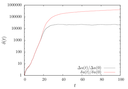
Figure 1: The divergence of the linear amplification and the nonlinear amplification of a perturbation with initial energy norm $\Delta u(0)=\delta u(0)=0.01$ (5)-(6) and the Reynolds number $Re=130$. $\delta(t)$ represents either $\frac{\Delta u(t)}{\Delta u(0)}$ or $\frac{\delta u(t)}{\delta u(0)}$. Divergence and nonlinear saturation happens around $t=20$ which is about $10$ large eddy turnover time $10T_{0}$.

In Figure 2, we show the nonlinear amplifications of perturbations for the Reynolds numbers $Re=130,805,1450,2520$. Except in $t\rightarrow 0^{+}$ limit, we clearly observed the amplifications of $e^{c\sqrt{t}}$ in $t$ as we predicted in (1). We use $c$ to represents a generic constant in this paper. In the $t\rightarrow 0^{+}$ limit, numerical resolution can never be sufficient and generates false results as shown by an explicit example in FL18 . Our extensive numerical simulations here and earlier show that the amplifications of $e^{c\sqrt{t}}$ in $t$ are generically observed FL18 .

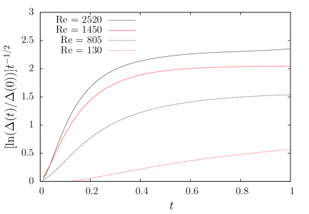
Figure 2: The nonlinear amplifications of perturbations for different Reynolds numbers $Re=130,805,1450,2520$. $\Delta(t)$ is the energy norm defined in (5). The horizontal portions of the curves represent amplifications of $e^{c\sqrt{t}}$ in $t$ as we predicted in (1).

In Figure 3, we show the dependence of the nonlinear amplifications of perturbations up to the time $t=0.3T_{0}$ on the Reynolds number, where $T_{0}$ is the large eddy turnover time which is around $2$. The data fit well with $e^{c\sqrt{Re}}$ as we predicted in (1). Thus both the $\sqrt{t}$ and the $\sqrt{Re}$ features in the exponent of our prediction (1) are verified here in the fully developed homogeneous isotropic turbulence regime.

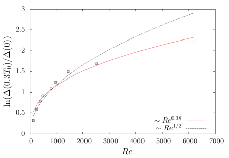
Figure 3: The Reynolds number dependence of the nonlinear amplifications of perturbations for different Reynolds up to the time $t=0.3T_{0}$, where $T_{0}$ is the large eddy turnover time which is around $2$. The dashed curve is a fit to $\sim\sqrt{Re}$, and the red (grey) curve is a fit to $\sim Re^{0.38}$.

In conclusion, built upon our earlier low resolution numerical verifications of our prediction (1) on the maximal amplification of perturbations in fully developed turbulence FL18 , here we conduct large direct numerical simulations with sufficient resolutions on fully developed homogeneous isotropic turbulence, and we have verified our prediction (1). In particular, our numerical simulations show that the amplification of perturbations behaves as $e^{c\sqrt{t}}$ in $t$ and $e^{c\sqrt{Re}}$ in $Re$ as we predicted in (1). Thus amplifications of perturbations in fully developed turbulence are much faster than exponential in contrast to the exponential amplifications of perturbations in chaos. Turbulence should appear more violent than chaos. Such superfast amplifications of perturbations naturally lead to superfast nonlinear saturations, and we have demonstrated such nonlinear saturations. We conclude that fully developed turbulence is generated, developed and maintained by such constant superfast amplifications of ever existing perturbations. We believe that this theory better explains what is observed in fully developed turbulence than the chaos theory.

We believe that our discovery here will better guide turbulence engineering, design and prediction such as the Ensemble Weather Forecasting in Meteorology.

- (1) Y. Li, Dynamics of PDE 10, 379 (2013).
- (2) Y. Li, Notices of the AMS 65, 1255 (2018).
- (3) D. Ruelle and F. Takens, Comm. Math. Phys. 20, 167 (1971).
- (4) T. Bohr, M. H. Jensen, G. Paladin, and A. Vulpiani, Dynamical Systems Approach to Turbulence (Cambridge University Press, 2005).
- (5) G. Kawahara and S. Kida, J. Fluid Mech. 449, 291 (2001).
- (6) D. Viswanath, J. Fluid Mech. 580, 339 (2007).
- (7) J. F. Gibson, J. Halcrow, and P. Cvitanović, J. Fluid Mech. 611, 107 (2008).
- (8) L. van Veen and G. Kawahara, Phys. Rev. Lett. 107, 114501 (2011).
- (9) G. Kawahara, M. Uhlmann, and L. van Veen, Ann. Rev. Fluid Mech. 44, 203 (2012).
- (10) T. Kreilos and B. Eckhardt, Chaos 22, 047505 (2012).
- (11) D. Lucas and R. Kerswell, Phys. Fluids 27, 045106 (2015).
- (12) D. Ruelle, Phys. Lett. 72A, 81 (1979).
- (13) A. Crisanti, M. H. Jensen, A. Vulpiani, and G. Paladin, Phys. Rev. Lett. 70, 166 (1993).
- (14) E. Aurell, G. Boffetta, A. Crisanti, G. Paladin, and A. Vulpiani, Phys. Rev. Lett. 77, 1262 (1996).
- (15) E. Aurell, G. Boffetta, A. Crisanti, G. Paladin, and A. Vulpiani, J. Phys. A 30, 1 (1997).
- (16) G. Boffetta, M. Cencini, M. Falcioni, and A. Vulpiani, Phys. Rep. 356, 367 (2002).
- (17) G. Boffetta and S. Musacchio, Phys. Rev. Lett. 119, 054102 (2017).
- (18) A. Berera and R. Ho, Phys. Rev. Lett. 120, 024101 (2018).
- (19) Y. Li, Electronic Journal of Differential Equations 2014, 104 (2014).
- (20) Y. Li, Nonlinearity 30, 1097 (2017).
- (21) H. Inci, Dynamics of Partial Differential Equations 12, 97 (2015).
- (22) H. Inci and Y. Li, arXiv preprint, arXiv:1805.06507 (2018).
- (23) Z. Feng and Y. Li, arXiv preprint, arXiv:1702.02993 (2018).
- (24) S. R. Yoffe, Ph.D. Thesis, University of Edinburg (2012), arXiv: 1306.3408.
- (25) L. Machiels, Phys. Rev. Lett. 79, 3411 (1997).
- (26) Y. Kaneda and T. Ishihara, J. of Turbulence 7, N20 (2006).
- (27) M. F. Linkmann and A. Morozov, Phys. Rev. Lett. 115, 134502 (2015).