Rare-Event Properties of the Nagel-Schreckenberg Model

Abstract

We have studied the distribution of traffic flow $q$ for the Nagel-Schreckenberg model by computer simulations. We applied a large-deviation approach, which allowed us to obtain the distribution $P(q)$ over more than one hundred decades in probability, down to probabilities like $10^{-140}$. This allowed us to characterize the flow distribution over a large range of the support and identify the characteristics of rare and even very rare traffic situations. We observe a change of the distribution shape when increasing the density of cars from the free flow to the congestion phase. Furthermore, we characterize typical and rare traffic situations by measuring correlations of $q$ to other quantities like density of standing cars or number and size of traffic jams.

I Introduction

The Nagel-Schreckenberg model for traffic flow is a cellular automaton model introduced in 1992 Nagel and M.Schreckenberg (1992). It is a very simple yet fundamental model not only for traffic but also for general transport phenomena and the occurrence of slow (glassy) dynamics de Wijn et al. (2012). This model has started in the statistical physics community a very active field of research on traffic Chowdhury et al. (2000a); Helbing (2001). To mimic human behavior in the model, which leads to fluctuations and in turn to the occurrence of spontaneous traffic jams, a stochastic component responsible for random speed reduction was introduced. The model undergoes a change of the behavior from free flow to congested traffic when the density of cars increases Nagel and M.Schreckenberg (1992), reminding of a phase transition. In the past years, a lot of research concerning this model was on the question, whether this transition is an example for a real non-equilibrium phase transition Chowdhury et al. (2000a); Eisenblätter et al. (1998); Roters et al. (1999); Chowdhury et al. (2000b).

So far in literature, the model was investigated, let it be analytically or numerically, regarding its typical behavior. Usually, the fundamental diagram, which shows the mean value of traffic flow $q$ as a function of the density of cars $\rho$ is studied. It shows a maximum at a density $\rho_{\max}$ Nagel and M.Schreckenberg (1992), which signifies the change from free flow to congested behavior. However, investigating typical behaviour only allows, from a fundamental point of view, to explore the model with a rather narrow focus.

Nevertheless, when describing any stochastic model as comprehensively as possible, one aims at obtaining the probability distributions of the quantities of interest over a large range of the support. This means one is interested in understanding the model beyond its typical properties down to rare events that only occur with very small probabilities, also called large deviations den Hollander (2000); Touchette (2009); Dembo and Zeitouni (2010); Touchette (2011).

Furthermore, for traffic models this is also of high practical interest, because even minor fluctuations can, with a small probability, lead to severe consequences like large traffic jams. Thus also rare events should be studied to understand them better and possibly help to plan traffic system such that costly traffic jams due to rare-event fluctuations are better avoided in real situations. Therefore, a large-deviation approach Hartmann (2014) based on a Monte Carlo (MC) simulation is applied here by which the measure $q$ can also be obtained in atypical regions. Thus, it enables one to obtain the distribution of the traffic flow $q$ over the full support, or at least a much larger range of values than standard approaches. We are able to resolve the distribution of $q$ in some cases over more than one 100 orders of magnitude, down to probability densities as small as $10^{-140}$.

It is the aim of this work to investigate whether the shape of the distribution of the traffic flow $q$, in particular its tail properties, changes at the transition from free to congested flow. The analysis of the distributions is done by approximating the tails with a fit function, and then studying the fit parameters as a function of the density of cars. In addition, the large-deviation approach enables us to investigate correlations between the traffic flow $q$ and other measures like the average jam size $S_{\rm av}$ or the density of jammed cars $\rho_{\text{jammed cars}}$ over a larger range of values. This allows us to characterize the atypical states of the system.

The paper is organized as follows. Next, we define the model and explain the numerical approaches we applied. In section III.1 the results for the distributions are presented and compared to results obtained from previous work Nagel and M.Schreckenberg (1992); Gerwinski and Krug (1999); Csanyi and Kertesz (1995). The results concerning correlations of $q$ with other values of interest are displayed in section III.2. We finish by a discussion and outlook in section IV.

II Model and Methods

The Nagel-Schreckenberg model, as studied here by computer simulations Hartmann (2015), is defined on an one-dimensional lattice with $L$ sites and periodic boundary conditions. Each car $i$ has a position $x_{i}\in\{0,1,...,L-1\}$ and a velocity $v_{i}\in\{0,1,...,v_{\max}\}$ with $v_{\max}$ being the speed limit. With the total number of cars $N$, the density of cars is

$$\rho=\frac{N}{L}$$ (1)

and the traffic flow $q$ (per lattice site) is given by

$$q=\frac{1}{L}\sum_{i=0}^{N-1}v_{i}\,.$$ (2)

The dynamics of the system is described by the following update-rules, that are applied one after the other, in parallel for all vehicles Nagel and M.Schreckenberg (1992):

1. Acceleration: if car $i$ has a velocity $v_{i}<v_{\max}$:

   $v_{i}\rightarrow v_{i}+1$

2. Slowing down due to other vehicles, preventing accidents: if the gap $d_{i}=x_{i+1}-x_{i}-1$ between a car $i$ and the preceding car $i+1$ is smaller than the velocity $v_{i}$ of car $i$:

   $v_{i}\rightarrow d_{i}$

3. Randomization: with probability $p$, the velocity $v_{i}$ of car $i$ changes to:

   $v_{i}\rightarrow\max\left(v_{i}-1,0\right)$

4. Movement: The position $x_{i}$ of car $i$ is updated:

   $x_{i}\rightarrow x_{i}+v_{i}$

For our simulations, we have chosen $v_{\max}=5$ as in the original publication, for convenience and $p=0.2$. The general results should not depend much on the choice of these values. Starting with any initial configuration, simulating the Nagel-Schreckenberg dynamics is straightforward and fast. To get a description of any quantities of interest, in particular of the traffic flow $q$, one has to measure the distribution of these quantities, e.g., $P(q)$. In a straight forward way, one could simulate the system over long times and collect sample values in histograms. This sampling according the natural probabilities we call simple sampling (sometimes also called importance sampling in the literature). The number $J$ of statistically independent samples, typically $J\sim 10^{5}-10^{9}$, gives an indication of how well the distributions can be sampled, the smallest probabilities which can be approximately obtained are $O(J^{-1})$. If one is interested in obtaining the distributions over a substantial part of the support, one needs to measure in regions where the probabilities are much smaller, like $\sim 10^{-50}$. Here large-deviations algorithms can be used.

For self-containedness, and to include the adaptations made for the present model, we include a brief description of the large-deviation approach used here, which was basically introduced previously Hartmann (2014) for the case of the distribution of work for an Ising model. For the present study we consider a sequence $\underline{Y}=(\underline{y}^{(0)},\underline{y}^{(1)},\ldots\underline{y}^{(n)})$ of traffic configurations ($\underline{y}$ consisting each of positions $\{x_{i}\}$ and velocities $\{v_{i}\}$), where the transitions $\underline{y}^{(t)}\to\underline{y}^{(t+1)}$ are according to the Nagel-Schreckenberg model presented above. We call $\underline{Y}$ a history. We assume that the initial configuration $\underline{y}^{(0)}$ is in a steady state, which can be obtained by performing a long-enough simulation starting from any configuration at a given density. Furthermore, we assume that $n$ is sufficiently large such that $\underline{y}^{(n)}$ is statistically independent of $\underline{y}^{(0)}$. Thus, when measuring the traffic flow $q=q(\underline{Y})$ (only) at the final configuration $\underline{y}^{(n)}$, one obtains a statistically independent measurement of $q$. To obtain $K$ independent values of $q$, instead of performing one very long simulation with measuring every $n$ steps, one can therefore also perform $K$ independent runs each generating a history $\underline{Y}$ of length $n$, all starting with the same initial configuration, but with statistically independent evolutions. This scheme will it make possible to apply the large-deviation approach as explained below. Since the value of $n$ will be chosen large enough, the fact that $\underline{y}^{(0)}$ is fixed plays no role. Now we discuss the choice of $n$. Figure 1 shows the distributions $P_{n}^{(0)}(q)$ for a system of size $L=1000$ and $\rho=0.13$ after repeatedly evolving the system for a $n$ number of steps starting from the same steady state configuration $\underline{y}^{(0)}$. The data shown in Figure 1 was obtained via simple sampling. For a small number $n$ of time steps, the histograms strongly depends on the fixed initial configuration, i.e., the histogram is very narrow (for $n=0$ it is a delta peak at $q(\underline{y}^{(0)})$). When increasing $n$, the histograms change considerable, in particular they become broader. This change with $n$ becomes weaker when increasing $n$ even more, representing increasing statistical independence of the measured values $q$ from the traffic flow of the initial configuration. The distributions are almost identical for $n=300$ and $n=500$. Therefore, $n=300$ should approximately correspond to the correlation time of the system since this seems to be the amount of time steps it takes the system to forget its initial configuration. Thus, $n=300$ is used throughout this work.

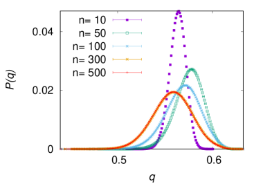
Figure 1: (color online) Distribution of the traffic flow $q$ for a system of size $L=1000$ and $\rho=0.13$ where repeatedly, starting always with the same (typical) configuration $\underline{y}^{(0)}$, statistically independent histories of $n$ steps were performed and then $q$ was measured each time after these $n$ steps. The distributions are shown for various number $n$ of steps.

Now, the main idea to access the low-probability tail is not to generate a sample with histories $\underline{Y}$, where each state occurs with its natural probability $R(\underline{Y})$ Hartmann (2011). Instead one samples according to a biased distribution Hammersley and Morton (1956); Bucklew (2004), where each history $\underline{Y}$ occurs with a probability taken as

$$R_{\theta}(\underline{Y})=\frac{1}{Z(\theta)}R(\underline{Y})e^{-q(\underline{Y})/\theta}$$ (3)

with a normalization factor $Z(\theta)$ and an artificial temperature $\theta$, see Ref. Hartmann (2011). The bias factor ${}^{-q(\underline{Y})/\theta}$ allows to control the range of sampled configurations via choosing $\theta$ appropriately. In particular for infinite temperate we recover simple sampling, i.e., we have $R_{\infty}(\underline{Y})=R(\underline{Y})$. When sampling configurations from $R_{\theta}(\underline{Y})$ and measuring $q=q(\underline{Y})$ one encounters a biased distribution $P_{\theta}(q)$ for the traffic flow $q$, depending on temperature $\theta$, which is given by Hartmann (2002)

$$P_{\theta}(q) =\sum_{\underline{Y}}R_{\theta}(\underline{Y})\delta_{q(\underline{Y}),q}$$

$$=\sum_{\underline{Y}}\frac{1}{Z(\theta)}R(\underline{Y})e^{-q(\underline{Y})/\theta}\delta_{q(\underline{Y}),q}$$

$$=\frac{e^{-q/\theta}}{Z(\theta)}\sum_{\underline{Y}}R(\underline{Y})\delta_{q(\underline{Y}),q}$$

$$=\frac{e^{-q/\theta}}{Z(\theta)}P(q),$$ (4)

with $P(q)=\sum_{\underline{Y}}R(\underline{Y})\delta_{q(\underline{Y}),q}$ being the actual target probability, i.e., the probability to measure a certain value of the traffic flow $q$ when each history $\underline{Y}$ occurs with its natural probability $R(\underline{Y})$ Hartmann (2011).

To generate histories $\underline{Y}$ according to $R_{\theta}(\underline{Y})$, we used the standard Metropolis-Hastings MC algorithm. Therefore, a Markov chain $\underline{Y}(0),\underline{Y}(1),\underline{Y}(2),\ldots$ of histories is created. This numbering of histories defines a second time in our simulation approach, the Markov-chain time $t_{\rm MC}$, not to be confused with the above inbtroduced time $t$ of the Nagel-SChreckenberg traffic evolution, which is relevant within each of the histories. In each step $t_{\rm MC}+1$, based on the current history $\underline{Y}(t_{\rm MC})$, a trial history $\underline{Y}_{\rm trial}$ with a traffic flow $q_{\rm trial}=q(\underline{Y}_{\rm trial})$ is generated. This involves for each $\underline{Y}_{\rm trial}$ a complete simulation of $n$ steps according the Nagel-Schreckenberg model and $q$ is measured for the final configuration. The trial history is accepted to be the next element of the Markov Chain, i.e., $\underline{Y}(t_{\rm MC}+1)=\underline{Y}_{\rm trial}$ with the Metropolis acceptance probability Hartmann (2014)

$$A(\underline{Y}\rightarrow\underline{Y}_{\rm trial})=\text{min}\left(1,e^{-[q(\underline{Y}_{\rm trial})-q(\underline{Y}(t_{\rm MC}))]/\theta}\right).$$ (5)

If the trial history is not accepted, the next history will be the current one, $\underline{Y}(t_{\rm MC}+1)=\underline{Y}(t_{\rm MC})$, as usually.

Next, we explain how we set up the simulation of a history, to incorporate it into the Markov chain Monte Carlo approach. In the randomization step (number 3), random numbers are necessary to determine the braking of cars. In every iteration, each car needs exactly one random number to decide whether to randomly decrease its velocity by one. In a typical implementation, one would call a pseudo random number generator function each time a random number is needed. In the large-deviation approach from Hartmann (2014), these random numbers are computed before performing the actual simulation Crooks and Chandler (2001) and stored in a vector $\underline{\xi}$. Whenever a random number is needed in the simulation, it is taken from $\underline{\xi}$. This approach is just a small, but necessary, technical adjustment, not at all altering the simulation result. Thus, the value of the measure, the traffic flow $q$, depends deterministically on this vector $\underline{\xi}$, since all randomness is subsumed here. Therefore, a Markov chain of histories $\underline{Y}(t_{\rm MC})$, given the initial configuration $\underline{y}^{(0)}$, is completely determined by a Markov chain of vectors $\underline{\xi}^{(t_{\rm MC})}$ ($t_{\rm MC}=0,1,2,\ldots$) because each history (at Monte Carlo time $t_{\rm MC}$) will start at the same configuration $\underline{y}^{(0)}$ and evolve for $n$ steps according $\underline{\xi}^{(t_{\rm MC})}$. Since each of the $N$ cars needs at each traffic time step $t$ exactly one random number, the vectors $\underline{\xi}$ covering all $n$ traffic time steps has size $n\times N$. The observable of interest is the traffic flow $q$ measured in the last time step, i.e., for $\underline{y}^{(n)}$.

To generate with the MC simulation a trial history $\underline{Y}_{\rm trial}$, correspondingly a trial vector $\underline{\xi}_{\rm trial}$ is constructed. We perform only small changes to obtain $\underline{\xi}_{\rm trial}$, thus we change only a small number of randomly selected entries of the current vector $\underline{\xi}(t_{\rm MC})$ Hartmann (2014). This is a local change to the current history, similar to a standard local spin-flip when simulating magnetic systems using Monte Carlo approaches. The amount of changed entries is variable. We have chosen it in a way that for each temperature $\theta$ approximately half of the trial histories get accepted Hartmann (2014), as a rule of thumb.

To ensure that the MC Simulation has equilibrated, the system is prepared with different initial histories $\underline{Y}(0)$. Technically, this is achieved by initializing the vector $\underline{\xi}(0)$ with random numbers with either a) all entries set to one, or b) with all entries set to zero, or c) with entries drawn from a uniform distribution in [0,1]. Figure 2 shows the measured values of the traffic flow $q$ (at the final configuration of each history, as always here) as a function of the Monte Carlo time $t_{MC}$ for a system with a very high density $\rho=0.8$ using different initializations. All curves reach, within fluctuations, the same value after a sufficient number of MC steps, proving the equilibration of the MC simulations. The curve corresponding to the initialization with all entries set to zero (which for our implementation means for the initial history the cars will always break for all traffic time steps, i.e., never accelerate) reaches equilibrium from below, whereas the curve corresponding to the initialization with all entries set to one (no spontaneous breaking initially) reaches the curve from above. Also for other values of $\rho$ and $\theta$ we have verified equilibration in a corresponding way.

Figure 2: Equilibration of the traffic flow $q$ as a function of the Monte Carlo time $t_{MC}$ for a system of size $L=1000$ and $\rho=0.8$ for an artificial temperature $\theta=0.3$.

After equilibration, the correct distribution $P(q)$ can be obtained from the measured biased distributions $P_{\theta}(q)$ (approximated by histograms) according to Eq. (4) by Hartmann (2014)

$$P(q)=e^{q/\theta}Z(\theta)P_{\theta}(q).$$ (6)

One has to perform simulations for several suitably chosen values $\theta_{1},\theta_{2},\ldots,\theta_{K}$, each focusing the simulation to a certain range of values of $q$. One can reconstruct $P(q)$ by combination of all results. The normalization constants $Z(\theta_{k})$ can be calculated Hartmann (2002) by a global normalization of $P(q)$ plus ensuring an overlap between the biased distributions $P_{\theta}(q)$ for neighboring values $\theta_{k},\theta_{k+1}$ and applying the condition $e^{q/\theta_{k}}Z(\theta_{k})P_{\theta_{k}}(q)=e^{q/\theta_{k+1}}Z(\theta_{k+1})P_{\theta_{k+1}}(q)$ for those values $q$ in the overlapping region, i.e., where one has good statistics for both $P_{\theta_{k}}(q)$ and $P_{\theta_{k+1}}(q)$. Clearly if several values of $q$ are contained in the overlapping region, the condition can only be approximately fulfilled simultaneously, e.g., by minimizing the mean-square deviation. For details see Refs. Hartmann (2002, 2011, 2014).

III Results

We have studied the Nagel-Schreckenberg model for system sizes between $L=100$ and $L=2000$, for eighteen different car densities $\rho\in[0.02,0.8]$. We used a maximum velocity $v_{\max}=5$ and a breaking probability $p=0.2$. All histories $\underline{Y}$, for each value of $\rho$ started with a precomputed steady-state configuration $\underline{y}^{(0)}$ of the corresponding density. For each history, the Nagel-Schreckenberg dynamics was performed for $n=300$ times steps, longer than the correlation time, and the traffic flow $q$ of the final configuration was measured. To obtain the distribution of these traffic flows, we performed MC simulations in the biased ensemble Eq. (3) for several values of the temperature parameter $\theta$ ranging from 8 different values for $L=100$ to 28 different values for $L=2000$. The length of the MC simulations was between $10^{4}$ MC steps for $L=100$ and $10^{9}$ steps for $L=1000$ (lowest density $\rho$). Due to long equilibration times for low densities and little finite size effects already for $L=1000$ for high and medium densities, the model was not investigated over the full support for $L=2000$ for very low densities.

First, we present below the results for the distributions of the traffic flow and for the corresponding rate functions. We fit the tails of the distributions to exponential functions and analyze the behavior of the fit parameters as a function of the car density $\rho$ and relate this to the fundamental diagram $\langle q\rangle(\rho)$. In the second section, we seek to establish a connection of the traffic-flow distributions to other values, i.e., ask the question what particular properties of traffic configurations are responsible for typical or particular small or high traffic flow.

III.1 Distributions and Rate Functions

Figure 3 shows the distributions $P(q)$ of the traffic flow $q$ for a system of size $L=1000$ for three different representative densities $\rho$. Figure 3 shows the behavior of $P(q)$ in the low density regime, here $\rho=0.02$, where a free flow is dominating. The simple sampling results are denoted by blue slightly large symbols. For the right tail, using our approach we were able to sample till the maximum possible flow. For small densities it is possible that all cars drive with maximum velocity $v_{\max}$. This determines the maximum via velocity times density. Note that for quite high densities this does not work any more and the maximum flow is determined by assuming that all free lattice sites are “visited” by a car, i.e., by the fraction of free lattice sites:

$$q_{\max}=\left\{\begin{array}[]{rl}v_{\max}\rho&\quad\mbox{for}\,\rho\,\mbox{small}\\ 1-\rho&\quad\mbox{for}\,\rho\,\mbox{large}\end{array}\right.\,.$$ (7)

For the left tail, even though not the full distribution was obtained in this regime due to too long equilibration times of the MC simulations, still a considerable large part of the support could be sampled by applying the large-deviation approach, down to probabilities like $10^{-38}$. In general, the results show, that the distribution is dominated by a peak very close to the maximum flow, but rare events with smaller flows occur.

Figure 3 shows the distribution near the transition. Because $q_{\max}$ is larger, the distribution covers a much larger range of the support compared to the low density result. Therefore, also much lower probabilities like $10^{-80}$ can be addressed. The distribution has a sharp bend in the typical regime and is stronger separated from the upper bound $q_{\max}$. Apart from that, the left tail already looks quite similar to the left tail of the distribution in the low-density case.

A typical distribution in the congested regime is displayed in Figure 3. Also in this regime, the distribution is asymmetric and exhibits a cut-off at the maximum flow $q_{\max}$. Nonetheless, the typical regime is even further apart from this value (as compared to lower densities) and hence the right tail covers a larger range of the support.

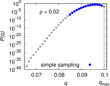
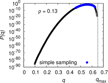
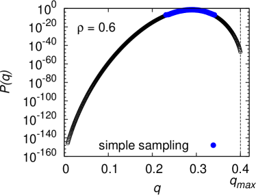
Figure 3: (color online) Probability distributions of the traffic flow $q$ for $L=1000$ for three different densities $\rho=0.02<\rho_{\max}$ (a), $\rho=0.13\approx\rho_{\max}$ (b) and $\rho=0.6>\rho_{\max}$ (c). The blue larger symbols indicate the result from simple sampling simulations. The vertical line at $q_{\max}$ indicates the maximum possible flow as given by Eq. (7)

In case the distribution exhibits the properties of the large deviation principle den Hollander (2000); Touchette (2009); Dembo and Zeitouni (2010); Touchette (2011) this roughly means that the probabilities are in the leading order exponentially small in the system size $L$, i.e., $P(q)\sim e^{-L\Phi(q)+o(L)}$. Thus, the empirical size dependent rate function Hartmann (2011)

$$\Phi(q)=-\frac{1}{L}\text{ ln}P(q)$$ (8)

(we omit the $L$ dependence on the left side for simplicity) just picks out $\Phi$ of this leading order and should converge for $L\to\infty$ if the large-deviation principle holds. In this case, a lot of relationships are known in large-deviation theory, such that, in principle, analytical results are easier accessible.

Figure 4 shows the resulting rate functions for the same densities $\rho=0.02$, $\rho=0.13$ and $\rho=0.6$, for different system sizes $L$. For increasing value of $L$, the empirical rate functions agree better and better Hartmann (2011), indicating a convergence. Therefore, the large-deviation principle seems to be fulfilled for all considered densities. The largest system sizes we can reach seem to be large enough to observe the limiting behavior rather well. Note, that the finite size effects seem to have the largest impact on the rate function for the medium density. This is due to a shift of the maximum of the fundamental diagram towards lower densities for larger system sizes and resembles the occurrence of stronger finite-size effects near phase transitions.

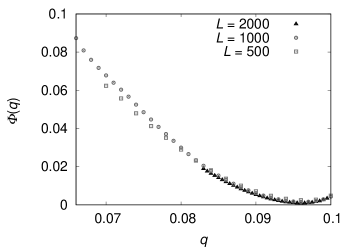
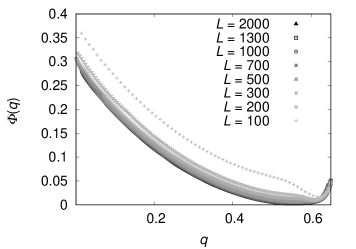
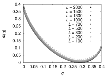
Figure 4: Empirical rate function $\Phi(q)$ for various system sizes $L$ and three different densities $\rho=0.02<\rho_{\max}$ (a), $\rho=0.13\approx\rho_{\max}$ (b) and $\rho=0.6>\rho_{\max}$ (c).

The shape of the rate functions hints that the tails might behave exponentially. This is confirmed by plotting the rate function with a logarithmically scaled $y$-axis, as shown in Figure 5. Therefore we have fitted the functions

$$f_{r}(q)=e^{C_{r}+m_{r}\cdot q}$$ (9)

with fit parameters $C_{r},m_{r}\in\mathbb{R}$ to the right tails and

$$f_{l}(q)=e^{C_{l}+m_{l}\cdot q}$$ (10)

with fit parameters $C_{l},m_{l}\in\mathbb{R}$ to the left tails of the rate functions data. The aim of this approach is to obtain fit parameters $m_{r}(\rho)$ and $m_{l}(\rho)$ for different densities $\rho$ and investigate thereby whether and how the transition from low (free flow) to high density (congested) regime affects the shape of the large-deviation tails. While the behavior in the typical regime is already well known by previous investigations of the fundamental diagram Chowdhury et al. (2000a), the impact of the transition on the entire distribution of the traffic flow $q$ has (to the authors’ knowledge) not been explored yet at all. Thus, to also investigate the atypical regime, the large-deviation tails are of particular interest. Figure 5 also shows examples for the obtained fit functions.

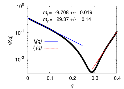
Figure 5: (color online) Empirical rate function for $L=1000$ and $\rho=0.6$. An exponential functions (9) and (10) have been fitted to the tails, yielding fit-parameters $m_{l}$ and $m_{r}$ describing the shape of the left and the right tails, respectively.

In order to investigate the system-size dependency of the fit parameters $m_{l}$ and $m_{r}$, we performed for two typical densities $\rho=0.13$ and $\rho=0.6$ the fits to the tails of the empirical rate function for all available system sizes $L$. Thus, for each size $L$, the parameters $m_{l}$ and $m_{r}$ were obtained. As an example, the parameter $m_{r}$ is shown for one density in Figure 6 as a function of $L$. Although we observe quite a bit of scatter for small system sizes $L$ (due to the fact that we display not directly measured values but fit parameters), the result does not change much for large system sizes, indicating a convergence for $L\to\infty$. To investigate this quantitatively, the function

$$f(L)=a+c\cdot L^{b}$$ (11)

is used as fit function for the data displayed in Figure 6, resulting in the displayed curve. The fit is not very good, which is anyway unavoidable due to the scatter of the data and the small error bars which are purely statistical. Nevertheless, for the shown example as well as for $m_{l}$, both for the two considered values of $\rho$, the values we have found for the largest system do not differ considerably from the extrapolated values (in terms of the general order of magnitude and the obtained error bars; although the actual values should not be taken too seriously). Thus, we just take the values of $m_{r}$ and $m_{l}$ obtained from the fits to the largest system sizes as good representatives of the exponential tail behavior of the rate functions for all eighteen different values of $\rho$ we have studied.

Figure 6: Fit parameter $m_{r}$ to the right tail as a function of the system size for a density $\rho=0.13$

Figure 7 shows the fundamental diagram (upper picture) and the fit parameters $m_{l}$ and $m_{r}$ for both tails (lower picture) as a function of the density of cars $\rho$. The maximum of the fundamental diagram is marked by a vertical dashed line. Both fit parameters exhibit an extreme value near the density $\rho_{\max}$ at which this maximum occurs.

A closer look reveals that the minimum of the fit parameter $m_{r}$ appears at a slightly higher density than the density $\rho_{\max}$ that maximizes the flow in the fundamental diagram. This reminds us of previous results Gerwinski and Krug (1999) obtained for the dissolution time $\tau_{J}$ of an initial mega jam, which shows a sharp increase near the critical density $\rho_{c}=\frac{1}{v_{\max}+1}$ at which the system exhibits a phase transition in the deterministic limit $p=0$.

Figure 7: Fundamental diagram (upper picture). The density of maximum flow $\rho_{\max}$ is marked by the dashed line. Fit parameters $m_{l}$ and $m_{r}$ as a function of the density of cars $\rho$ (lower picture). Both parameters exhibit an extreme value near the density of maximum flow.

This motivated us, to compare our results also with this jam dissolution time $\tau_{J}$ (which we obtained from separate standard simulations), which is shown in the upper picture of Figure 8 as a function of the density of cars $\rho$. The lower picture shows the fit parameter $m_{r}$ for the same range of densities $\rho$. In both cases, the same system of size $L=1000$ was used. One can see that the position of the minimum of $m_{r}$ lies in the range where $\tau_{J}$ increases strongly and closer to the the critical density $\rho_{c}=\frac{1}{v_{\max}+1}$ of the deterministic limit. A reason for this behavior is not obvious to us in the moment.

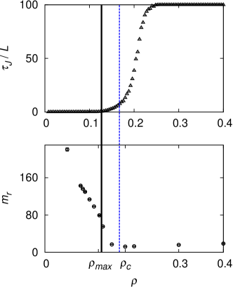
Figure 8: The upper picture shows the dissolution time $\tau_{J}$ of an initial mega jam. The density $\rho_{\max}$ that marks the maximum of the fundamental diagram and the critical density $\rho_{c}$ of the deterministic limit $p=0$ are marked by dashed lines. The lower picture shows the fit parameter $m_{r}$ as a function of the density of cars $\rho$.

Next, we have a closer look at the parameter $m_{l}$, as displayed in Figure 9. This parameter also exhibits an extreme value, which is, as mentioned above, at another density than the minimum of the fit parameter $m_{r}$. Since the relaxation time $\tau$ (see Csanyi and Kertesz (1995)) is known to exhibit a maximum at a density below $\rho_{\max}$, it is displayed in the upper picture of Figure 9. We observe (from additional simple sampling simulations) a maximum at some value $\rho_{\tau_{\max}}$. Since the slope of the curve is quite low in this region and the scattering of the data points in comparison is rather high, one cannot exactly determine the peak’s position precisely. But it appears to be located slightly below the value of $\rho_{\max}$ in agreement with the previous results Csanyi and Kertesz (1995). Nevertheless, with the current precision of our data we cannot decide whether the maximum of $m_{l}$ coincides rather with the maximum of the relaxation time $\rho_{\tau_{\max}}$ or with the position of maximum of the fundamental diagram $\rho_{\max}$, both appears to be possible. Nevertheless, the general results holds, that the tails of the distribution change considerably closely to the density where the change from the free-flow to the congested regime occurs.

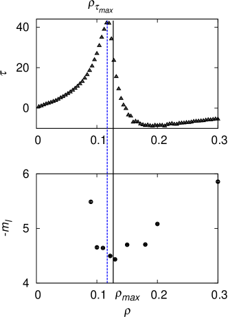
Figure 9: The relaxation time $\tau$ (see Ref. Csanyi and Kertesz (1995); upper figure) and the fit parameter $m_{l}$ for the left tail of the distribution function as a function of the car density $\rho$. The density $\rho_{\max}$ that marks the maximum of the fundamental diagram and the density $\rho_{\tau{\max}}$ at which $\tau$ exhibits its maximum are marked by dashed lines.

III.2 Correlations

Since we have access even to the extremest traffic situations which are possible under each given circumstances, it is worth asking whether there are other characteristics properties of these rare situations, in addition to extreme small or large values of the flow $q$. Thus, during our simulations we also measured and stored other quantities of interest, as stated below. This allows us to correlate them within our analysis with the observed traffic flow. Since our approach allows us to access the tails of the distributions, we are therefore able to investigate the correlations also over a very large range, much beyond the typical correlations. Understanding these correlations also for the extreme cases, might help to foster (or avoid) (un-)desired traffic situations in real cases. We concentrate the results we show on the region in the phase disgram near $\rho_{\max}$. For very low densities and very high densities, the correlations look typically very simple (or not much different from the presented), thus they are not discussed further here.

Figure 10 displays the correlation between the traffic flow $q$ and the density $\rho_{\text{standing cars}}$ of standing cars by a scatter plot. The results obtained by using the simple sampling approach are marked in blue. One can clearly see that the large-deviation approach allows us to investigate the correlations over a much wider range of the support. One can formulate a simple bound for these correlations: At a given density $\rho_{\text{standing cars}}$ of standing cars, the largest possible value for the traffic flow $q$ would be measured when all non-standing cars had maximum velocity $v_{\max}$ (which often might still not be possible), hence

$$\rho_{\text{standing cars}}=\rho-\frac{q}{v_{\max}}$$ (12)

is an upper bound for the density of standing cars at a given value of $q$. In Figure 10, a very strong correlation between $\rho_{\text{standing cars}}$ and $q$ is visible, with only a rather small scattering band. This means that the observed value of $q$ can be explained to a large extend by the fraction of standing cars, even in the rare-event region. Note that the data points approach the limit Eq. (12) for $q\rightarrow 0$. The reason for this behavior might be that a high number of standing cars means more space for the still unjammed cars, which therefore can have higher velocities. However, this would only be the case when the jammed cars were in the same local area, hence if there were a few large jams. This is indeed the case, as will be pointed out below.

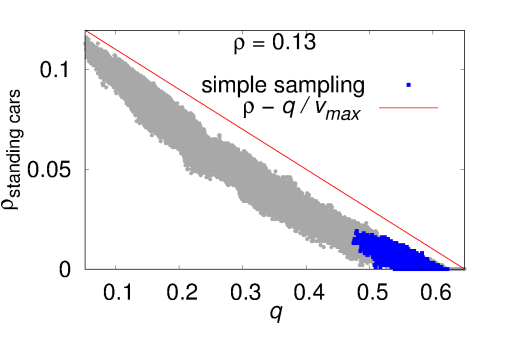
Figure 10: (color online) Scatter plot for correlation between the traffic flow $q$ and the density $\rho_{\text{standing cars}}$ of cars with velocity zero for a system of size $L=1000$ with $\rho=0.13$. The dark blue points indicate the data which can be found by simple sampling. The line indicates the maximum possible density $\rho_{\text{standing cars}}$ as function of $q$.

There are different ways of defining if a car is jammed, see Chowdhury et al. (2000a). Hereinafter, a car is defined jammed when it had to brake to zero due to another vehicle ahead. Therefore, the density of jammed cars equals the density $\rho_{\text{pairs}}$ of next neighbor pairs. A jam is therefore given by a cluster of standing cars with no gaps. Correspondingly the number $N_{\rm jams}$ of jams is the number of these clusters. Figure 11 shows the relation between $N_{\rm jams}$ and the traffic flow $q$. Very high values of the flow $q$ can only occur if the number of jams is small or even zero. For intermediate values of the traffic flow a broad range of the number of jams is possible, but typically more jams occur, with a maximum near $q=0.15$. For $q\rightarrow 0$, only a small number of jams can be observed. Since the density of jammed cars $\rho_{pairs}$ increases in this case (not displayed), this means that this (for this value of $\rho$) very extreme traffic situation is dominated by few but large jams.

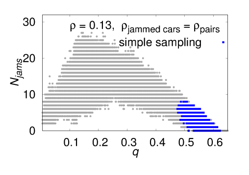
Figure 11: (color online) Scatter plot showing the correlation between the traffic flow $q$ and the number $N_{\rm jams}$ of jams for a system of size $L=1000$ and $\rho=0.13$. The dark blue points indicate the data which can be found by simple sampling.

To analyze the behavior observed in the preceding scatter plots, we show in Figure 12 the correlation between the number $N_{\rm jams}$ of jams and the average jam size $S_{\rm av}$. The average traffic flow $q$ for any pair $(S_{\rm av},N_{\rm jams})$ is coded by a gray scale. Again, we can derive a simple bound: If $S_{\rm av}$ is the average number of next neighbor pairs, $S_{\rm av}+1$ is the average amount of cars contained in jams (clusters) originating from these pairs. Since the maximum amount of jammed cars is the total number of cars $N$, the number $N_{\rm jams}$ of jams is limited by

$$N_{\rm jams}=N/(S_{\rm av}+1).$$ (13)

This boundary is marked by a red line in Figure 12. Accordingly, data points close to this line correspond to low values of the traffic flow $q$. The observed reverse ”U”-shape of the correlation plot between the number $N_{\rm jams}$ of jammed cars and the traffic flow $q$ from Figure 11 can also be observed here. Moreover, when being presented this way, one can directly see that a large number of jams corresponds to small jam sizes and intermediate values of $q$. An example traffic configuration is visualized in Figure 13. Furthermore a low number of jams can either correspond to a low average jam size and a high traffic flow $q$, see example configuration in Figure 14, or to a large average jam size and a low traffic flow $q$, see Figure 15.

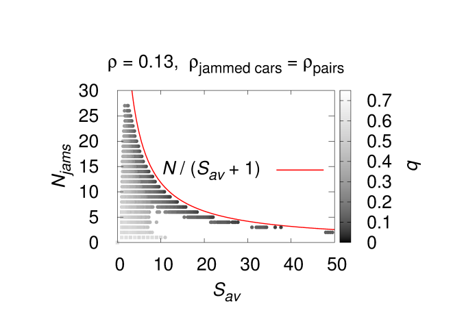
Figure 12: (color online) Scatter plot showing the correlation between the number $N_{\rm jams}$ of jams and the average jam size $S_{\rm av}$ of close cars for a system of size $L=1000$ and $\rho=0.13$. The line displays the simple bound from Eq. (13).

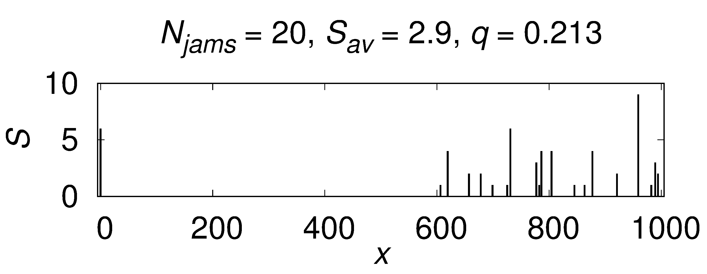
Figure 13: Example configuration for a medium traffic flow value $q$ for a system of size $L=1000$ and $\rho=0.13$. All jams starting at position $x$ and having size $S$ are indicated by vertical lines at positions $x$ and of height $S$.

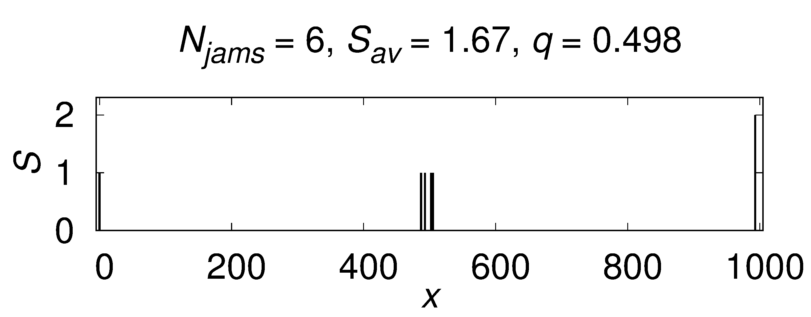
Figure 14: Example configuration for a high traffic flow value $q$ for a system of size $L=1000$ and $\rho=0.13$. All jams starting at position $x$ and having size $S$ are indicated by vertical lines at positions $x$ and of height $S$.

Figure 15: Example configuration for a low traffic flow value $q$ for a system of size $L=1000$ and $\rho=0.13$. All jams starting at position $x$ and having size $S$ are indicated by vertical lines at positions $x$ and of height $S$.

IV Discussion and Conclusion

We have studied the distributions of traffic flow $q$ for the Nagel-Schreckenberg model, i.e., for a non-equilibrium model, for various values of the car density $\rho$. By applying a sophisticated large-deviations approach, we are able to obtain $P(q)$ over a large range of the support, down to probabilities as small as $10^{-140}$. First, this is satisfying from a fundamental research point of view, because only knowing the full (or almost full) distribution contains the full information for a stochastic system. Second, the approach allows to investigate the reasons of the occurrences of large deviations by correlating the main quantity of interest, here $q$, to other measurable values, like the number or sizes of jams. Third, also in real traffic systems seemingly rare events may occur. Give the fact that there are millions of kilometers of roads worldwide cia (2019) and that traffic situations change from minute to minute several times, a rough estimates shows that within a year even events exhibiting a probability like $10^{-13}$ actually occur on a global scale. Events exhibiting such probabilities are also difficult to simulate using a standard approach. Thus, for practical purposes also medium-small probabilities which are accessible using the large-deviation approach might be of practical interest.

In the present work, we have analyzed the distribution of the flow, starting from a steady-state configuration after a rather long evolution of $n=300$ time steps. We have shown that on the level of the distribution of the flow, the initial configuration of cars and speeds is mostly forgotten. Thus we basically analyzed the large-deviation properties of the steady state, at least for low-enough densities.

Note that it could be indeed also of interest to study deliberately the distributions of flow after a smaller number $n$ of steps, to investigate the statistical properties of the traffic evolution over small time intervals, and correspondingly the dependence on the initial configuration which should be more pronounced. This could be an interesting aspect for further studies.

The fundamental question of the present work is whether there is a correspondence between the shape and large-deviation properties of the distribution of the flow (order) parameter and the phase or state the system is in. Such correspondences have been observed previously for phase transitions in equilibrium models, like the percolation transition of random graphs Engel et al. (2004); Hartmann (2011, 2017); Hartmann and Mézard (2018); Schawe and Hartmann (2019). For the Nagel-Schreckenberg model, we find exponential left and right tails in $P(q)$ for all cases, but the slope of the tails changes significantly. The distribution exhibits the smallest slopes near the change from free flow to the congested phase. Thus, also here, for a non-equilibrium model, we see such a strong relationship between phase and shape and tail properties of the distribution of the “order parameter”.

Furthermore, our correlation analysis reveals that in the onset of the congested region near the “critical” density $\rho_{\max}$, non unexpectedly, the correlation between the flow and number of standing cars is very straightforward (this holds also for other values of $\rho$). Nevertheless, with respect to the number of traffic jams, the situation is more complex. Although a large number of jams, which occurs for this density with a small probability, corresponds to an already significantly reduced flow, a smaller number of jams can occur for large flow (small jams), which is typical for this density, and for small flow (large jams), which is an extreme event here.

For the present study we started always with a typical steady-state configuration as initial configuration of any history. Here, e.g., traffic jams are very unlikely for very small densities $\rho$ (and become more and more likely when increasing $\rho$). Thus, it could be interesting to use other more atypical, but still realistic, initial configuration, which may be seen as precursors of traffic jams or other events. Then one could again analyze the distributions $P(q)$ which will probably lead to increased traffic jam probability. This could lead to a more precise prediction of unlikely traffic situations, conditioned to different initial configurations.

Also, the traffic flow is not the only quantity of interest, where one can apply the large-devaition approach. Also for other quantities like the number or the duration of traffic jams it could be of interest to obtain the probability distribution over a large or full range of the support. Clearly, these distributions can not be read off from the present results, because independent MC simulations with biases driven by the quantities of interest have to be used.

Finally, it is obvious that we have applied the large-deviation approach to a very simple traffic model, e.g., it exhibits just one lane, no in- or outflow, a homogeneous type of cars and drivers. We have chosen such a very simple model to provide a proof of principle, to show that the large-deviation approach allows for insights beyond those accessible by standard simple sampling. Hence, for further studies it would be certainly interesting to apply our approach also to more complex, i.e., more realistic traffic models.