Effective Training of Convolutional Neural Networks with Low-bitwidth Weights and Activations

Abstract

This paper tackles the problem of training a deep convolutional neural network of both low-bitwidth weights and activations. Optimizing a low-precision network is very challenging due to the non-differentiability of the quantizer, which may result in substantial accuracy loss. To address this, we propose three practical approaches, including (i) progressive quantization; (ii) stochastic precision; and (iii) joint knowledge distillation to improve the network training. First, for progressive quantization, we propose two schemes to progressively find good local minima. Specifically, we propose to first optimize a network with quantized weights and subsequently quantize activations. This is in contrast to the traditional methods which optimize them simultaneously. Furthermore, we propose a second progressive quantization scheme which gradually decreases the bit-width from high-precision to low-precision during training. Second, to alleviate the excessive training burden due to the multi-round training stages, we further propose a one-stage stochastic precision strategy to randomly sample and quantize sub-networks while keeping other parts in full-precision. Finally, we adopt a novel learning scheme to jointly train a full-precision model alongside the low-precision one. By doing so, the full-precision model provides hints to guide the low-precision model training and significantly improves the performance of the low-precision network. Extensive experiments on various datasets (e.g., CIFAR-100, ImageNet) show the effectiveness of the proposed methods.

1 Introduction

State-of-the-art deep neural networks  [1, 2, 3] usually involve millions of parameters and need billions of FLOPs for training and inference. The significant memory consumption and computational cost can make it intractable to deploy models to mobile, embedded hardware devices. To improve computing and memory efficiency, various solutions have been proposed, including network pruning [4, 5, 6], low rank approximation of weights [7, 8], training a low-precision network [9, 10, 11, 12] and efficient architecture design [13, 14, 15]. In this work, we follow the idea of training a low-precision network and our focus is to improve the training process of such a network. Thus, our work targets the problem of training a network with both extremely low-bit weights and activations.

The solutions proposed in this paper contain three components. They can be applied independently or jointly. The first component is the progressive quantization which consists of two schemes. The first strategy is to adopt a two-stage training process. At the first stage, only the weights of a network are quantized. After obtaining a sufficiently good solution at the first stage, the activation of the network is further required to be in low-precision and the network is trained again. Essentially, this two-stage approach first solves a related sub-problem, i.e., training a network with only low-bit weights and the solution of the sub-problem provides a good initial point for training our target problem. Following the similar idea, we propose our second scheme by performing progressive training on the bitwidth aspect of the network. Specifically, we incrementally train a serial of networks with the quantization bitwidth (precision) gradually decreased from full-precision to the target precision.

However, the above progressive quantization needs several retraining steps which introduces additional training burdens. To solve this problem, we further propose our second component termed stochastic precision to effectively combine these two strategies into one single training stage. Inspired by dropout strategies [16, 17], we randomly select a portion of the model (e.g., layers, blocks) and activations or weights to quantize while keeping other parts in full-precision. Thus, we can improve the gradient flow for effectively training quantized neural networks.

The third component is inspired by the recent progress of information distillation [18, 19, 20, 21, 22]. The basic idea of those works is to train a target network alongside another guidance network. For example, the works in [18, 19, 20, 21, 22] propose to train a small student network to mimic the deeper or wider teacher network. They add an additional regularizer by minimizing the difference between student’s and teacher’s posterior probabilities [19] or intermediate feature representations [22, 18]. It is observed that by using the guidance of the teacher model, better performance can be obtained with the student model than directly training the student model on the target problem. Motivated by these observations, we propose to train a full-precision network alongside the target low-precision network. In our work, the student network has the similar topology as that of the teacher network, except that the student network is low-precision while the teacher network keeps full-precision operations. Moreover, in contrast to standard knowledge distillation methods, we allow the teacher network to be jointly optimized with the student network rather than being fixed since we discover that this strategy enables the two networks adjust better to each other. Interestingly, the performance of both the full-precision teacher and the low-precision student can be improved.

Our main contributions are summarized as follows.

• We propose two progressive quantization schemes for tackling the non-differentiability of quantization operations during training. In the first scheme, we propose a two-stage training manner, where the weights are first quantized to serve as a good initialization on further quantizing activations. In the second scheme, we progressively reduce the bitwidth during training to find better local minima.

• To reduce the extra training burden, we introduce structured stochastic training, leading to an effective, simplified one-stage training approach.

• To our knowledge, we are the first to propose to improve the low-precision network training using knowledge distillation technique where the full-precision teacher and the quantized student are jointly optimized to adapt to each other. We explore different distilling schemes in Sec. 4 and all produce improved accuracy for the low-precision model.

• We conduct extensive experiments with various precisions and architectures on the image classification task.

This paper extends the preliminary conference version [23] in several aspects. 1) Although the multi-stage progressive quantization in [23] clearly improves the performance, the multiple re-initialization and fine-tuning steps make the training procedure complex and introduce computation overhead. To solve this problem, here we propose a much simpler one-stage stochastic precision strategy that enjoys the advantage of the multi-stage progressive quantization. 2) We extend the hint-based joint knowledge distillation to a more advanced framework that unifies attention transfer [21] and posterior-based schemes. 3) We now conduct extensive experiments on ImageNet over various architectures to formulate strong and comprehensive baselines for future works. We study several schemes which produce low-precision networks using different distilling strategies and provide interesting analysis.

2 Related work

We have witnessed a growing interest of model compression methods, such as limited numerical precision, efficient architecture design and knowledge distillation. We also study the dropout strategies in this paper. Next we discuss related literature with respect to these aspects.

Limited numerical precision. Model quantization aims to quantize the weights, activations and even backpropagation gradients into low-precision, to yield highly compact DNNs compared to their floating-point counterparts. As a result, most of the multiplication operations in network inference can be replaced by more efficient addition or bitwise operations. In general, quantization methods generally involve binary neural networks (BNNs) and fixed-point quantization. In particular, BNNs [24, 25, 26, 27, 28, 29, 30], where both weights and activations are quantized to binary tensors, are reported to have potentially $32\times$ memory compression ratio, and up to $58\times$ speed-up on CPU compared with the full-precision counterparts. However, BNNs still suffer from sizable performance drop issue, hindering them from being widely deployed. To make a trade-off between accuracy and complexity, researchers also study fixed-point quantization [12, 31, 32, 33, 34]. In general, quantization algorithms aim at tackling two core challenges. The first challenge is to design accurate quantizers to minimize the information loss. Early works use handcrafted heuristic quantizers [12] while later studies propose to adjust the quantizers to the data, basically based on matching the original data distribution [12, 35], minimizing the quantization error [36] or directly optimizing the quantizer with stochastic gradient descent [31, 37]. The second challenge is to approximate gradients of the non-differentiable quantizer. To solve this problem, most works in literature simply employ “pseudo-gradients” according to the straight-through estimator (i.e., STE) [38]. Some recent studies propose to improve the discrete optimization problem via loss-aware training [39], regularization [40, 41, 42], entropy maximization [43, 44], or smoothing the quantizer [45]. In addition to the quantization algorithms design, the underlying implementation and acceleration libraries [46, 47, 48, 49] are indispensable to expedite the quantization technique to be deployed on energy-efficient edge devices. In this paper, we propose three training solutions that can be built upon general quantization approaches.

Efficient architecture design. The increasing demand for highly energy efficient neural networks that are deployable to embedded hardware devices has motivated the network architecture design. SqueezeNet [50] replaces $3\times 3$ convolutional filters with $1\times 1$ size, which significantly decreases the complexity. Depthwise separable convolutions employed in Xception [51], MobileNet [14] and ShuffleNet [15] have been proved to be efficient and effective. Since it is infeasible to manually explore the optimal architecture from the enormous design space, neural architecture search (NAS) aims at automating the architecture design, giving rise to methods based on the reinforcement learning [52, 53, 54, 55], evolutionary algorithms [56], or gradient-based methods [57, 58, 13].

Moreover, network pruning [4, 59] can be viewed as a special case of NAS, aiming to remove redundant connections such as convolutional filters. Some works also employ reinforcement learning [60, 61], Bayesian optimization [62] or NAS [63] to automatically search the pruning policy for each layer.

Knowledge distillation. Knowledge distillation was initially proposed for model compression, where a powerful wide/deep teacher distills knowledge into a narrow/shallow student to improve its performance [18, 19]. In terms of the representation of knowledge to be distilled from the teacher, existing models typically use teacher’s class probabilities [19] and/or feature representations [18, 21]. Knowledge distillation has been widely used in many computer vision tasks. Zhang et al.   [64] proposes to transfer the knowledge learned with optical flow CNN to improve the action recognition performance. Moreover, several works propose to learn efficient object detection [65, 66] and semantic segmentation [67] with distillation. In contrast to previous approaches, we concentrate on improving the performance of the quantized neural network. By adapting the teacher and student altogether, we can steadily improve the performance of the quantized student network and even the full-precision teacher network. Note that concurrent works  [68, 44] with ours [23] also apply knowledge distillation to quantization. We have also explored it together with other advanced training strategies.

Dropout. Dropout [16], Maxout [69], DropConnect [70] and DropIn [71] are a category of approaches that stochastically drop intermediate nodes or connections during training to prevent the network from overfitting. They essentially perform different types of regularization. Huang et al.   [17] further propose stochastic depth regularization via randomly dropping a subset of layers during training. Dong et al.   [72] proposes to randomly quantize a portion of weights to low-precision in the incremental training framework [9]. The method in [72] was developed for only quantizing weights of a network. In our method, we develop an extension of it by further randomly quantizing a portion of the network, i.e., layers or blocks as well as activations and weights. Moreover, we [23] propose two progressive training strategies: 1) quantizing weights and activations in a two-stage manner; 2) progressively decreasing the bitwidth from high-precision to low-precision during the course of training. However, the multi-stage strategy may slow down the training. Inspired by those dropout approaches, we improve the progressive quantization by proposing an efficient single-stage stochastic precision strategy. Our study shows that this extended scheme is complementary to the proposed joint knowledge distillation approach.

Recently, Yu et al.  proposed slimmable neural networks [73, 74] aiming to train a single neural network executable at different widths on the fly at test time, permitting instant and adaptive accuracy-efficiency trade-offs. The core challenge is to sufficiently train all sub-networks. Specifically, the original slimmable neural networks [73] proposes to average gradients of different widths without introducing stochastic selection. To improve the optimization of all sub-networks, US-Nets [74] randomly samples widths in a certain range and apply averaged gradients back-propagated from the accumulated loss. However, our approach aims to solve the notorious difficulty in propagating gradients through a low-precision network due to the non-differentiable quantization function. Inspired by the dropout strategies, we propose to stochastically quantize a portion of the network to low-bit while keeping the other portion full-precision, thus making gradients back-propagate more easily. In our method, there is no “sub-networks” concept. We aim to maximize the performance of the whole quantized network rather than optimizing the mixed-precision network stochastically generated in each iteration sufficiently.

3 Methods

In this section, we first introduce the quantization preliminaries in Sec. 3.1. We then describe the progressive quantization schemes in Sec. 3.2 and explain the stochastic precision approach in Sec. 3.3. Finally, we elaborate the joint knowledge distillation in Sec. 3.4.

3.1 Problem definition

In this work, we use DoReFa-Net [12] to quantize both weights and activations. Consider the general case of $k$-bit quantization. We define the quantization function $Q(\cdot)$ as:

$$z_{q}=Q(z)=\frac{1}{2^{k}-1}\cdot{\rm{round}}((2^{k}-1)\cdot z_{r}),$$ (1)

where ${z_{r}}\in[0,1]$ denotes the normalized full-precision value and ${z_{q}}\in[0,1]$ denotes the normalized quantized value. With this quantization function, we can define the weight quantization process and the activation quantization process as follows:

Quantization on weights:

$${w_{q}}=2Q\left(\frac{{\tanh(w)}}{{2\max(\left|{\tanh(w)}\right|)}}+\frac{1}{2}\right)-1.$$ (2)

In other words, we first use $\frac{{\tanh(w)}}{{2\max(\left|{\tanh(w)}\right|)}}+\frac{1}{2}$ to obtain a normalized version of $w$ and then perform the quantization, where $\tanh(\cdot)$ is adopted to reduce the impact of large values.

Quantization on activations:

Same as [12], we first use a clip function $f(x)={\rm{clip}}(x,\,0,1)$ to bound the activations to $[0,1]$. After that, we quantize the activation by applying the quantization function $Q(\cdot)$ on $f(x)$:

$${x_{q}}=Q(f(x)).$$ (3)

Back-propagation with quantization function:

In general, the quantization function is non-differentiable and thus it is impossible to directly apply the back-propagation to train the network. To overcome this issue, we adopt the straight-through estimator [12, 25, 38] to approximate the gradients calculation. Formally, we approximate the partial gradient $\frac{{\partial{z_{q}}}}{{\partial{z_{r}}}}$ with an identity mapping, namely $\frac{{\partial{z_{q}}}}{{\partial{z_{r}}}}\approx 1$. Accordingly, $\frac{{\partial\ell}}{{\partial{z_{r}}}}$ can be approximated by

$$\frac{{\partial\ell}}{{\partial{z_{r}}}}=\frac{{\partial\ell}}{{\partial{z_{q}}}}\frac{{\partial{z_{q}}}}{{\partial{z_{r}}}}\approx\frac{{\partial\ell}}{{\partial{z_{q}}}},$$ (4)

where $\ell$ is the loss.

3.2 Progressive quantization

3.2.1 Two-stage optimization

With the straight-through estimator, it is possible to directly optimize the low-precision network. However, the gradient approximation of the quantization function inevitably introduces noisy signals for updating network parameters. Strictly speaking, the approximated gradient may not be the right updating direction. Thus, the training process can be more likely to get trapped at a poor local minimal than training a full-precision model. Applying the quantization function to both weights and activations further worsens the situation.

To alleviate this training difficulty, we devise a two-stage optimization procedure as follows. At the first stage, we only quantize the weights of the network while setting the activations to be full-precision. After the converge (or after a certain number of iterations) of this model, we further apply the quantization function on the activations as well and retrain the network. Essentially, the first stage of this method is a related sub-problem of the target one. Compared to the target problem, it is easier to optimize since it only introduces quantization function on weights. Thus, we are more likely to arrive at a good solution for this sub-problem. Then, using it to initialize the target problem may help the network avoid poor local minima which is likely to be encountered if we train the network from scratch.

Let $M_{\rm{low}}^{K}$ be the high-precision model with $K$-bit. We propose to learn a low-precision model $M_{\rm{low}}^{k}$ in a two-stage manner with $M_{\rm{low}}^{K}$ serving as the initial point, where $k<K$. The detailed algorithm is shown in Algorithm 1.

Input: Training data $\{({{\mathbf{x}}_{i}},y_{i})\}_{i=1}^{N}$; A $K$-bit precision model $M_{\rm{low}}^{K}$ with weights ${\mathbf{W}}_{\rm{low}}^{K}$.

Output: A low-precision deep model $M_{\rm{low}}^{k}$ with weights ${\mathbf{W}}_{\rm{low}}^{k}$ and activations being quantized into $k$-bit.

1

2Stage 1: Quantize ${\mathbf{W}}_{\rm{low}}^{K}$:

3 for $\mathrm{epoch}=1,...$ do

4       for $i=1,...N$ do

5             Randomly sample a mini-batch data;

6             Quantize the weights ${\mathbf{W}}_{\rm{low}}^{K}$ into $k$-bit by calling some quantization methods with $K$-bit activations;

7            

8      

9 Stage 2: Quantize activations:

10 Initialize ${\mathbf{W}}_{\rm{low}}^{k}$ using the converged $k$-bit weights from Stage 1 as the starting point;

11 for $\mathrm{epoch}=1,...$ do

12       for $i=1,...N$ do

13             Randomly sample a mini-batch data;

14             Quantize the activations into $k$-bit by calling some quantization methods while keeping the weights to $k$-bit;

15      

Algorithm 1 Two-stage optimization for $k$-bit quantization

3.2.2 Progressive precision

The aforementioned two-stage optimization approach suggests the benefits of using a relatively easy-to-optimize problem to find a good initialization. However, separating the quantization of weights and activations is not the only solution to implement the above idea. In this paper, we also propose a second scheme which progressively lowers the bitwidth of the quantization during the course of network training. Specifically, we progressively conduct the quantization from higher precisions to lower precision (e.g., 32-bit $\to$ 16-bit $\to$ 4-bit $\to$ 2-bit). The model of higher precision will be used as the starting point of the relatively lower precision, in analogy with annealing.

Let $\{{b_{1}},...,{b_{n}}\}$ be a sequence precision, where $b_{n}<b_{n-1},...,b_{2}<{b_{1}}$, $b_{n}$ is the target precision and $b_{1}$ is set to 32 by default. The whole progressive optimization procedure is summarized in Algorithm 2.

Let $M_{\rm{low}}^{k}$ be the low-precision model with $k$-bit and $M_{\rm{full}}$ be the full-precision model. In each step, we propose to learn $M_{\rm{low}}^{k}$, with the solution in the $(i-1)$-th step, denoted by $M_{\rm{low}}^{K}$, serving as the initial point, where $k<K$.

Input: Training data $\{({{\mathbf{x}}_{j}},y_{j})\}_{j=1}^{N}$; A pre-trained 32-bit full-precision model $M_{\rm{full}}$ as baseline; the precision sequence $\{{b_{1}},...,{b_{n}}\}$ where $b_{n}<b_{n-1},...,b_{2}<{b_{1}}=32$.

Output: A low-precision deep model $M_{\rm{low}}^{b_{n}}$.

1 Let $M_{\rm{low}}^{b_{1}}=M_{\rm{full}}$, where $b_{1}=32$;

2 for $i=2,...n$ do

3       Let $k=b_{i}$ and $K=b_{i-1}$;

4       Obtain $M_{\rm{low}}^{k}$ by calling some quantization methods with $M_{\rm{low}}^{K}$ being the input;

5      

Algorithm 2 Progressive precision for accurate CNNs with low-precision weights and activations

3.3 Stochastic precision

In the proposed progressive quantization method, we need to gradually quantize the network to low-precision in multi-round training stages. However, the multiple re-initialization and fine-tuning steps may introduce additional computation overhead. To solve this problem, this section develops a single-stage stochastic precision (SP) strategy to improve the training efficiency while enjoying the advantage of the multi-stage progressive quantization. Inspired by the studies that incrementally or stochastically train a certain part of the network [9, 73], we propose to incorporate the stochasticity into the progressive training.

The term “stochastic structure” means that we randomly choose a network structural component, namely, layers, blocks, activations or weights to quantize and keep the rest to be full-precision. The specific scheme is elaborated as follows.

Suppose that we decompose the network $M$ into $Z$ fragments $M=\{{m_{1}},...,{m_{Z}}\}$, where ${m_{i}}$ can be any structure such as a convolutional layer or a residual block. For each iteration, we intend to partition the fragments into two sets, a low-precision set ${G_{q}}=\{{m_{q_{1}}},...,{m_{q_{N_{q}}}}\}$ and a full-precision set ${G_{r}}=\{{m_{r_{1}}},...,{m_{r_{N_{r}}}}\}$, which satisfies the condition:

$${G_{q}}\cup{G_{r}}=M,\ \mathrm{and}\ {G_{q}}\cap{G_{r}}=\emptyset.$$ (5)

where $N_{q}$ and $N_{r}$ are the number of elements in two sets respectively.

In our method, we randomly partition $M_{\rm{low}}$ into $G_{q}$ and $G_{r}$. This is implemented by introducing a binary indicator ${\mathbf{b}}\in{\mathbb{R}^{Z}}$ and a stochastic ratio $\delta$. We randomly set ${\mathbf{b}}(i)=1$ with probability $(1-\delta)$, and if ${\mathbf{b}}(i)=1$ the $i$-th fragment is quantized and otherwise is kept to be full-precision. We linearly decrease $\delta$ to 0 to ensure the whole network being quantized in the end. Note that this procedure implicitly achieves the effect of the incremental quantization [9] but without the need of multi-round training.

To further increase the randomness in quantizing $m$, we can stochastically choose whether to quantize weights or activations or both of them. This can be implemented by randomly sampling a binary indicator matrix ${\bf{B}}\in{\mathbb{R}^{Z\times 2}}$, where its first column is used to decide whether to quantize the weights in the corresponding fragment and the second column is used to decide whether to quantize activations respectively.

As a result, $G_{q}$ can be further partitioned into three subsets $\{{G_{qwa}},{G_{qw}},{G_{qa}}\}$, which represents quantizing both weights and activations, only quantizing weights and only quantizing activations, respectively. Thus, SP can share the advantage of the progressive training in Sec. 3.2.1 and Sec. 3.2.2.

Moreover, in Sec. 4.2.1, we will explore the effect of different structure choices of $m$ as well as the extent of randomness to the final performance.

Input: Training data $\{{{\mathbf{x}}^{t}},{{\mathbf{y}}^{t}}\}$; weights ${\mathbf{W}}^{t}$ (${\mathbf{W}}^{0}$ = ${\mathbf{W}}_{\rm{full}}$); stochastic ratio $\delta^{t}$ and decay rate $\mu$.

Output: Updated parameters ${\mathbf{W}}^{t+1}$; stochastic ratio $\delta^{t+1}$.

1 Partition $M$ into $Z$ fragments $\{{m_{1}},...,{m_{Z}}\}$;

2 if $\delta^{t}>0$ then

3       Obtain the binary indicator matrix ${\mathbf{B}}^{t}$ via uniform sampling with probability $\delta^{t}$;

4       Partition the network $M$ into the quantized set $G_{q}=\{{G_{qwa}^{t}},{G_{qw}^{t}},{G_{qa}^{t}}\}$ and the full-precision set $G_{r}^{t}$ according to ${\bf{B}}^{t}$;

5       Obtain the corresponding mixed-precision parameter set $\widetilde{\mathbf{W}}^{t}=\{Q({{\mathbf{W}}^{t}_{qwa}}),Q({{\mathbf{W}}^{t}_{qw}}),{{\mathbf{W}}^{t}_{qa}},{{\mathbf{W}}^{t}_{r}}\}$ ;

6

7else

8      $\widetilde{\mathbf{W}}^{t}=Q({\mathbf{W}}^{t})$;

9

10${{\mathbf{\widetilde{y}}}^{t}}=\mathrm{Forward}({{\mathbf{x}}^{t}},\widetilde{\mathbf{W}}^{t})$;

11 Compute the loss ${\cal L}({{\mathbf{y}}^{t}},\widetilde{\mathbf{y}}^{t})$;

12 $\frac{{\partial{\cal L}}}{{\partial{\widetilde{\mathbf{W}}^{t}}}}=\mathrm{Backward}(\frac{{\partial{\cal L}}}{{\partial{{\mathbf{\widetilde{y}}}^{t}}}},{\widetilde{\mathbf{W}}^{t}})$;

13 Update parameters ${\mathbf{W}}^{t+1}$ using STE defined in Eq. (4) and some proper optimizers;

$\delta^{t+1}=\delta^{t}-\mu$;

Algorithm 3 Stochastic precision training algorithm.

3.4 Joint knowledge distillation on quantization

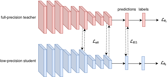
Figure 1: Demonstration of the guided training strategy. Dashed lines show the guidance loss.

The third approach proposed here is inspired by the success of using information distillation  [18, 19, 20, 21, 22] to train a relatively shallow network. Specifically, these methods usually use a teacher model (usually a pretrained deeper network) to provide guided signal for the shallower network. Following this motivation, we propose to train the low-precision network alongside another guidance network. Unlike the work in [18, 19, 20, 21, 22], the guidance network shares the similar architecture as the target network but is pretrained with full-precision weights and activations.

However, a pre-trained model may not be necessarily optimal or may not be suitable for quantization. As a result, directly using a fixed pretrained model to guide the target network may not produce the best guidance signals. To mitigate this problem, we do not fix the parameters of a pretrained full-precision network.

By using the guidance training strategy, we assume that there exist some full-precision models with good generalization performance, and an accurate low-precision model can be obtained by directly performing the quantization on those full-precision models. In this sense, the feature maps of the learned low-precision model should be close to that obtained by directly performing quantization on the full-precision model. To achieve this, essentially, in our learning scheme, we can jointly train the full-precision and low-precision models. This allows these two models adapt to each other. We even find by doing so the performance of the full-precision model can be slightly improved in some cases.

Input: Training data $\{({\mathbf{x}}_{i},y_{i})\}_{i=1}^{N}$; A pre-trained 32-bit full-precision model $M_{\rm{full}}$; A $k$-bit precision model $M_{\rm{low}}^{k}$.

Output: A low-precision deep model $M_{\rm{low}}^{k}$ with weights and activations being quantized into $k$ bits.

1 Initialize $M_{\rm{low}}^{k}$ based on $M_{\rm{full}}$;

2 for $\mathrm{epoch}=1,...$ do

3       for $i=1,...N$ do

4             Randomly sample a mini-batch data;

5             Quantize the weights ${\mathbf{W}}_{\rm{low}}$ and activations into $k$-bit by minimizing ${\cal L}_{2}({\mathbf{W}}_{\rm{low}})$;

6             Update $M_{\rm{full}}$ by minimizing ${\cal L}_{1}({\mathbf{W}}_{\rm{full}})$;

7            

8      

Algorithm 4 Guided training with a full-precision network for $k$-bit quantization

Formally, let ${\mathbf{W}}_{\rm{full}}$ and ${\mathbf{W}}_{\rm{low}}$ be the weights of the full-precision model and low-precision model, respectively. Let $\mu({\mathbf{x}};{\mathbf{W}}_{\rm{full}})$ and $\nu({\mathbf{x}};{\mathbf{W}}_{\rm{low}})$ be the nested feature maps (i.e., activations) of the full-precision model and low-precision model, respectively. To create the guidance signal, we may require that the nested feature maps from the two models should be similar. However, $\mu({\mathbf{x}};{\mathbf{W}}_{\rm{full}})$ and $\nu({\mathbf{x}};{\mathbf{W}}_{\rm{low}})$ is usually not directly comparable since one is full-precision and the other is low-precision. To link these two models, we can directly quantize the weights and activations of the full-precision model. For simplicity, we denote the quantized feature maps by $Q(\mu({\mathbf{x}};{\mathbf{W}}_{\rm{full}}))$. Thus, $Q(\mu({\mathbf{x}};{\mathbf{W}}_{\rm{full}}))$ and $\nu({\mathbf{x}};{\mathbf{W}}_{\rm{low}})$ will become comparable. Inspired by the attention transfer method [21], we propose to apply attention matching at a set of $\mathcal{T}$ transfer points within a network, the constraint can be expressed as:

$${\cal L}_{att}({\mathbf{W}}_{\rm{full}},{\mathbf{W}}_{\rm{low}})=\sum\limits_{i=1}^{N}\sum\limits_{j=1}^{\mathcal{T}}\left\lVert\frac{\mathcal{A}^{j}_{S}}{\parallel\mathcal{A}^{j}_{S}\parallel_{2}}-\frac{\mathcal{A}^{j}_{T}}{\parallel\mathcal{A}^{j}_{T}\parallel_{2}}\right\rVert,$$ (6)

where $\mathcal{A}^{j}_{S}$ and $\mathcal{A}^{j}_{T}$ are the sum of the absolute values across the channel dimension of feature maps $\nu({\mathbf{x}}_{i};{\mathbf{W}}_{\rm{low}})$ and $Q(\mu({\mathbf{x}}_{i};{\mathbf{W}}_{\rm{full}}))$, respectively.

Similar to [19], we can also employ the posterior probability as the guidance signal. Let ${\mathbf{p}}_{\rm{full}}$ and ${\mathbf{p}}_{\rm{low}}$ be the full-precision teacher network and low-precision student network predictions, respectively. To measure the correlation between the two distributions, we employ the Kullback–Leibler (KL) divergence:

$${{\cal L}_{\rm{KL}}}({\mathbf{p}}_{\rm{full}}|{\mathbf{p}}_{\rm{low}})=\sum\limits_{i=1}^{N}{{\mathbf{p}}_{\rm{full}}({\mathbf{x}}_{i})}\log\frac{{{{\mathbf{p}}_{\rm{full}}}({{\mathbf{x}}_{i}})}}{{{{\mathbf{p}}_{\rm{low}}}({\mathbf{x}}_{i})}}.$$ (7)

Finally, let ${{\cal L}_{{\theta_{1}}}}$ and ${{\cal L}_{{\theta_{2}}}}$ be the cross-entropy classification losses for the full-precision and low-precision model, respectively. The guidance losses in Eqs. (6) and (7) will be added to ${{\cal L}_{{\theta_{1}}}}$ and ${{\cal L}_{{\theta_{2}}}}$, respectively, resulting in the final objectives for the two networks, namely

$${{\cal L}_{1}}({\mathbf{W}}_{\rm{full}})=\alpha_{1}{{\cal L}_{{\theta_{1}}}}+\beta{{\cal L}_{\rm{KL}}}({\mathbf{p}}_{\rm{low}}|{\mathbf{p}}_{\rm{full}})+\gamma{\cal L}_{att}({\mathbf{W}}_{\rm{full}},{\mathbf{W}}_{\rm{low}}),$$ (8)

and

$${{\cal L}_{2}}({\mathbf{W}}_{\rm{low}})=\alpha_{2}{{\cal L}_{{\theta_{2}}}}+\beta{{\cal L}_{\rm{KL}}}({\mathbf{p}}_{\rm{full}}|{\mathbf{p}}_{\rm{low}})+\gamma{\cal L}_{att}({\mathbf{W}}_{\rm{full}},{\mathbf{W}}_{\rm{low}}),$$ (9)

where $\{\alpha_{1},\alpha_{2}\}$, $\beta$ and $\gamma$ are the balancing hyper-parameters. We share $\beta$ and $\gamma$ for these two objectives.

In the learning procedure, both ${\mathbf{W}}_{\rm{full}}$ and ${\mathbf{W}}_{\rm{low}}$ will be updated by minimizing ${\cal L}_{1}({\mathbf{W}}_{\rm{full}})$ and ${\cal L}_{2}({\mathbf{W}}_{\rm{low}})$ separately, using a mini-batch stochastic gradient descent method. The detailed algorithm is shown in Algorithm 4. A high-bit precision model $M_{\rm{low}}^{K}$ is used as an initialization of $M_{\rm{low}}^{k}$, where $K>k$. Specifically, for the full-precision model, we have $K=32$. Relying on $M_{\rm{full}}$, the weights and activations of $M_{\rm{low}}^{k}$ can be initialized respectively.

Note that the training process of the two networks are different. When updating ${\mathbf{W}}_{\rm{low}}$ by minimizing ${\cal L}_{2}({\mathbf{W}}_{\rm{low}})$, we use the full-precision model as initialization and apply STE to fine-tune the model. When updating ${\mathbf{W}}_{\rm{full}}$ by minimizing ${\cal L}_{1}({\mathbf{W}}_{\rm{full}})$, we use conventional forward-backward propagation to fine-tune the model.

3.5 Remarks on the proposed methods

The proposed three approaches tackle the difficulty in training a low-precision model with different strategies. They can be applied independently. However, it is also possible to combine them together. For example, we can apply the progressive precision to any step in the two-stage approach; we can also apply the joint knowledge distillation to any step in the progressive quantization; we can combine stochastic precision with the joint knowledge distillation approach. Detailed analysis on possible combinations will be empirically evaluated in the experiment section.

4 Experiments

Datasets and models. To investigate the performance of the proposed methods, we conduct experiments on CIFAR-100 [75] and ImageNet [76]. We employ ResNet [3], PreResNet [77] and AlexNet [1] for experiments. We use a variant of the AlexNet structure by removing dropout layers and add batch normalization after each convolutional layer and fully-connected layer. This structure is widely used in previous works [12, 11].

Comparison methods. To justify the effectiveness of the proposed approaches, we conduct experiments on various representative quantization approaches, including uniform fixed-point approach DoReFa-Net [12], non-uniform fixed-point method LQ-Net [36], as well as binary neural network approaches BiReal-Net [30] and Group-Net [33]. The “Baseline” in all experiments means that we quantize the model using DoReFa-Net [12], which is defined in Sec. 3.1. We define “TS”, “PP”, “SP” and “KD” to represent two-stage optimization in Sec. 3.2.1, progressive precision in Sec. 3.2.2, stochastic precision in Sec. 3.3 and joint knowledge distillation in Sec. 3.4, respectively.

Implementation details. As in [24, 35, 12, 23, 33], we quantize the weights and activations of all convolutional layers except that the first and the last layers are kept in full-precision. However, we also quantize all the layers so that the model contains complete fixed-point operations and we label this case with a * symbol. In all ImageNet experiments, training images are resized to $256\times 256$, and a $224\times 224$ crop is randomly sampled from an image or its horizontal flip, with the per-pixel mean subtracted. We do not use any further data augmentation in our implementation. We use a simple single-crop testing for standard evaluation. No bias term is utilized.

Without loss of generality, we finetune from the pretrained full-precision model and set the initial learning rate for the quantized model to 0.005. We train a maximum 30 epochs, and decay the learning rate by 10 at the 15-th and 25-th epoch. We use SGD for optimization, with a batch size of 256, a momentum of 0.9 and a weight decay of 1e-4. More specific hyperparameters are provided in each subsection. Our implementation is based on PyTorch.

4.1 Effect of progressive quantization

In this part, we explore the effect of the proposed progressive quantization methods.

4.1.1 Effect of the two-stage optimization

We analyze the effect of each stage in the two-stage approach in Figure 2. We take the 2-bit ResNet-50 on ImageNet as an example. In Figure 2, step-1 has the minimal loss of accuracy. As for the step-2, although it incurs an apparent accuracy decrease in comparison with that of the step-1, its accuracy is consistently better than the results of the baseline in every epoch. This illustrates that progressively seeking for the local minimum point is crucial for final better convergence, which proves the effectiveness of this simple mechanism.

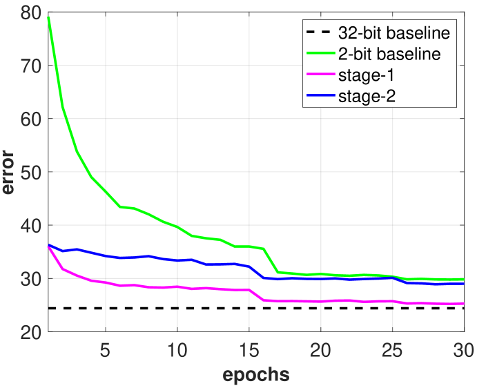
Figure 2: The two-stage training approach on ResNet-50.

TABLE I: Accuracy (%) of different comparing methods on the ImageNet validation set.

Precision	model	method	top-1 acc.	top-5 acc.
2W, 2A	ResNet-50	Baseline	70.19	89.15
		Baseline + TS	70.92	90.03
		Baseline + PP	70.78	89.98
		Baseline + TS + PP	71.13	90.12
4W, 4A	ResNet-50*	Baseline	75.11	75.70
		Baseline + TS	75.32	91.93
		Baseline + PP	75.38	91.77
		Baseline + TS + PP	75.50	92.01
2W, 2A	ResNet-50*	Baseline	67.68	70.00
		Baseline + TS	69.22	87.03
		Baseline + PP	68.79	86.90
		Baseline + TS + PP	69.43	87.01
4W, 4A	AlexNet*	Baseline	56.17	79.35
		Baseline + TS	57.66	81.03
		Baseline + PP	57.47	80.80
		Baseline + TS + PP	57.83	80.85
2W, 2A	AlexNet*	Baseline	48.26	71.56
		Baseline + TS	50.67	74.92
		Baseline + PP	50.29	74.80
		Baseline + TS + PP	50.94	74.93

4.1.2 Effect of the progressive precision strategy

What is more, we also separately explore the progressive precision effect on the final performance. In this experiment, we apply AlexNet and ResNet-50 on the ImageNet dataset. We continuously quantize both weights and activations simultaneously from 32-bit$\to$8-bit$\to$4-bit$\to$2-bit and explicitly illustrate the accuracy change process for each precision in Figure 3. The quantitative results are also reported in Table I. From the figure, we find that for 8-bit and 4-bit, the low-bit model has no accuracy loss with respect to the full-precision model. However, when quantizing from 4-bit to 2-bit, we can observe a significant accuracy drop. Despite this, we still observe $2.0\%$ relative improvement by comparing the Top-1 accuracy over the 2-bit baseline, which proves the effectiveness of the proposed strategy. It is worth noting that the accuracy curves become more unstable when quantizing to the lower bit. This phenomenon is reasonable because the quantized value will change more frequently during the training process when the bitwidth is reduced.

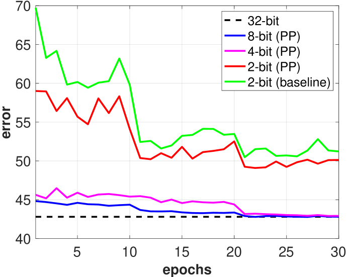
Figure 3: The progressive training approach on AlexNet*.

4.2 Effect of the stochastic precision

In this subsection, we further explore the effect of the stochastic precision strategy on general quantization approaches. The stochastic ratio $\delta$ is initialized to 0.5 and linearly decayed to 0 at the 20-th epoch. We train a maximum 40 epochs and decay the learning rate by 10 at the 25-th and 35-th epochs. Other hyperparameters are set to default. The default structure of the fragment $m$ is a residual block and we stochastically quantize weights and activations in all cases unless special explanations. The results are reported in Table II. By combining the baseline methods with SP, we find an apparent performance increase compared with the baselines in all cases. During training, we stochastically keep a portion of the network to full-precision and update by the standard gradient-based method. This strategy shares the similar spirit with the progressive quantization to relax the discrete quantizer effectively. Moreover, the proposed stochastic strategy only requires one training stage without fine-tuning the model in many training rounds.

TABLE II: Accuracy (%) of different comparing methods with SP on the ImageNet validation set. Experiments are repeated for 3 times and we report the results with mean and standard deviation.

model	method	top-1 acc.	top-5 acc.
ResNet-50	DoReFa-Net (2-bit)	70.19	89.15
	DoReFa-Net + SP	72.23$\pm$0.05	90.78$\pm$0.10
ResNet-50	LQ-Net (3-bit)	74.23	91.63
	LQ-Net + SP	75.14$\pm$0.04	92.33$\pm$0.09
ResNet-18	BiReal-Net	56.43	79.52
	BiReal-Net + SP	58.81$\pm$0.05	81.24$\pm$0.12
ResNet-18	GroupNet (5 bases)	64.82	85.72
	GroupNet + SP	65.89$\pm$0.06	86.30$\pm$0.10

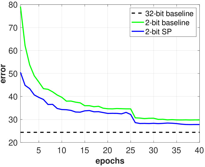
Figure 4: The stochastic precision training approach on ResNet-50.

4.2.1 Effect of different SP policies

We further explore the influence of different choices of the fragment $m$ described in Sec. 3.3 as well as the extent of randomness. We treat GroupNet as our baseline approach and utilize 5 binary bases. The results are reported in Table III. We explore two different structures of $m$, including one convolutional layer and one residual block which corresponds to layerdrop and blockdrop respectively. We further incorporate the randomness of quantizing weights and activations into $m$ and is denoted by W/A. From the results, we observe that all the four cases show improved performance compared with the baseline, which justifies adding randomness is a general way for relaxing the low-precision network training. By comparing the result of layerdrop+W/A with layerdrop, we observe performance drop with the increase of randomness. However, blockdrop+W/A performs slightly better than blockdrop. This shows that adding excessive stochasticity can make the gradient updating direction deviate while appropriate extent of randomness can relax the non-differentiable problem to facilitate optimization. Moreover, the accuracy of layerdrop and blockdrop are very close, which shows that the structure of $m$ is not sensitive to the final performance.

TABLE III: Accuracy (%) of different stochastic policies on the ImageNet validation set.

model	method	top-1 acc.	top-5 acc.
ResNet-18	GroupNet (5 bases)	64.8	85.7
	GroupNet + blockdrop	65.6	86.3
	GroupNet + layerdrop	65.7	86.5
	GroupNet + blockdrop + W/A	65.9	86.6
	GroupNet + layerdrop + W/A	65.0	86.1

4.3 Effect of the joint knowledge distillation on quantization

To investigate the effect of the joint knowledge distillation approach explained in Sec. 3.4, we explore four different training schemes to obtain a low-precision student network.

4.3.1 Joint fine-tuning of the low-precision student and the full-precision teacher

In this scheme, both networks are primed with corresponding full-precision pretrained weights as initialization and are jointly optimized. We explore two network structures, including PreResNet and ResNet. When using a certain student network $M_{\rm{low}}$, we use the teacher network $M_{\rm{full}}$ to have either the same or larger depth. The results are reported in Table IV and Table V. The initial learning rates for $M_{\rm{low}}$ and $M_{\rm{full}}$ are set to be 0.005 and 0.001, respectively. The balancing hyperparameters $\{\alpha_{1},\alpha_{2}\}=\{1,0.5\}$, $\beta=0.5$ and $\gamma=50$. Other hyperparameters are set to default.

Discussion. From the results, we observe that all our low-precision models surpass the corresponding baselines. It justifies that $M_{\rm{full}}$ can provide useful auxiliary supervision to assist the convergence of $M_{\rm{low}}$. Moreover, the relative improvement with ResNet is larger than that with PreResNet. To highlight, the relative Top-1 improvement w.r.t.  2-bit ResNet-50 is 1.77% while the PreResNet-50 counterpart is 0.71%. This phenomenon can be attributed that quantized ResNet is more difficult to be optimized since the skip connections are also quantized which blocks layers later in the network to access information gained in earlier layers. In this scenario, $M_{\rm{full}}$ can effectively ease the training of $M_{\rm{low}}$ by adapting knowledge to each other. We can also justify that keeping the skip connections to high-precision is important to maintain the performance of the low-precision network similar to [30, 78].

Moreover, we can come to an assumption that the distillation process becomes more effective when the low-precision network is more difficult to train. This assumption can be further proved by the experiments in Sec. 4.3.2.

In Table V, we experiment with PreResNet-18 which is paired with various teacher networks but with deeper layers. However, the benefit of using a deeper network saturates at some points. For example, the final trained accuracy of 2-bit PreResNet-18 model paired with PreResNet-50 is only 0.04% higher than that obtained by pairing the PreResNet-34 network.

With the simple DoReFa-Net uniform quantization strategy, we can achieve comparable or even higher accuracy compared with the full-precision model using 4-bit precision. It means that we can deploy the 4-bit model in hardware devices with no loss of accuracy which would greatly save memory bandwidth and power consumption.

Interestingly, we also observe that the full-precision teacher can also be improved by learning together with the student. We plot the convergence curves in Figure 5. We can observe that the teacher’s performance drops at the beginning epochs due to inaccurate gradients from the student. During optimization, the student network serves as a regularizer for the teacher network which can even surpass the pretrained baseline.

TABLE IV: Accuracies of the quantized ResNet using joint training approach and finetuning. W and A refer to the bitwidth of weights and activations, respectively. Experiments are repeated for 3 times and we report the results with mean and standard deviation.

Precision		ResNet-18 Baseline	ResNet-18 with ResNet-18	ResNet-34 Baseline	ResNet-34 with ResNet-34	ResNet-50 Baseline	ResNet-50 with ResNet-50
32W, 32A	Top-1%	69.75	-	73.21	-	75.64	-
	Top-5%	89.01	-	91.40	-	92.25	-
4W, 4A	Top-1%	69.47$\pm$0.04	70.18$\pm$0.04	71.31$\pm$0.03	73.08$\pm$0.05	74.50$\pm$0.03	75.67$\pm$0.06
	Top-5%	88.80$\pm$0.09	90.20$\pm$0.12	90.08$\pm$0.11	91.53$\pm$0.10	91.46$\pm$0.14	92.19$\pm$0.13
2W, 2A	Top-1%	64.67$\pm$0.04	65.58$\pm$0.05	68.17$\pm$0.05	69.20$\pm$0.06	70.19$\pm$0.04	71.96$\pm$0.06
	Top-5%	85.78$\pm$0.10	86.44$\pm$0.14	88.05$\pm$0.09	89.09$\pm$0.13	89.15$\pm$0.08	90.63$\pm$0.16

TABLE V: Accuracies of the quantized PreResNet using joint training approach and finetuning. Experiments are repeated for 3 times and we report the results of mean and standard deviation.

Precision		PreResNet-18 Baseline	PreResNet-18 with PreResNet-18	PreResNet-18 with PreResNet-34	PreResNet-18 with PreResNet-50	PreResNet-34 Baseline	PreResNet-34 with PreResNet-34	PreResNet-50 Baseline	PreResNet-50 with PreResNet-50
32W, 32A	Top-1%	69.95	-	-	-	73.53	-	76.11	-
	Top-5%	89.21	-	-	-	91.30	-	92.81	-
4W, 4A	Top-1%	69.81$\pm$0.04	70.12$\pm$0.05	-	-	73.57$\pm$0.03	73.90$\pm$0.03	75.92$\pm$0.02	76.62$\pm$0.04
	Top-5%	89.04$\pm$0.09	89.57$\pm$0.09	-	-	91.35$\pm$0.08	91.62$\pm$0.10	92.82$\pm$0.07	93.14$\pm$0.09
2W, 2A	Top-1%	64.51$\pm$0.05	65.67$\pm$0.06	65.82$\pm$0.05	65.86$\pm$0.04	69.31$\pm$0.05	70.26$\pm$0.04	71.20$\pm$0.04	71.91$\pm$0.05
	Top-5%	85.85$\pm$0.10	86.80$\pm$0.11	86.84$\pm$0.10	86.73$\pm$0.12	88.92$\pm$0.11	89.64$\pm$0.10	90.18$\pm$0.10	90.53$\pm$0.12

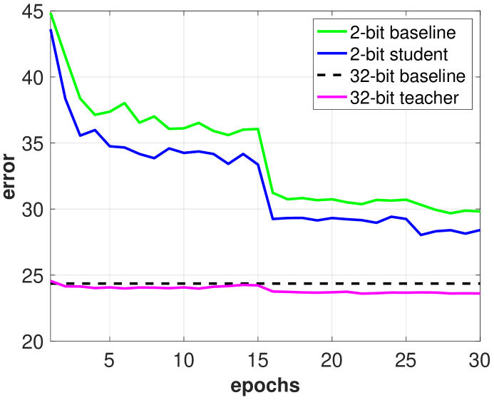
Figure 5: Both student and teacher are fine-tuned from the pretrained models. We use ResNet-50 as illustration.

4.3.2 Learning from scratch vs. fine-tuning

In this scheme, we train a low-precision student from scratch given a pretrained full-precision teacher network. During training, both of the models are mutually updated. The initial learning rates for student and teacher are set to be 0.1 and 0.001, respectively. We train a maximum 80 epochs with SGD, and the learning rate is decayed by 10$\times$ at epochs 30, 50, 60 and 70. We use the batch size of 256.

The results are reported in Table VI. From the results, we can summarize two instructive statements.

• The relative improvement of KD is more apparent than those that are from fine-tuning. For instance, with 2-bit representations, the relative improvement for PreResNet-50 is 2.40% while the fine-tuning counterpart is 0.71% in Table V. This is reasonable since learning from scratch is more challenging than fine-tuning and the auxiliary guidance from the teacher has more affects.

• Fine-tuning performs steadily better than learning from scratch. It shows that the pretrained full-precision model can serve as an important initialization.

We also show the convergence curves in Figure 6.

TABLE VI: The accuracy of the quantized PreResNet using the joint training approach, which is learnt from scratch. Experiments are repeated for 3 times and we report the results with mean and standard deviation.

Precision		PreResNet-18 Baseline	PreResNet-18 with PreResNet-18	PreResNet-34 Baseline	PreResNet-34 with PreResNet-34	PreResNet-50 Baseline	PreResNet-50 with PreResNet-50
32W, 32A	Top-1%	69.95	-	73.53	-	76.11	-
	Top-5%	89.21	-	91.30	-	92.81	-
4W, 4A	Top-1%	67.85$\pm$0.08	69.29$\pm$0.10	71.46$\pm$0.13	73.05$\pm$0.14	73.82$\pm$0.12	75.42$\pm$0.11
	Top-5%	88.15$\pm$0.16	88.84$\pm$0.15	90.06$\pm$0.14	91.01$\pm$0.16	91.53$\pm$0.13	92.82$\pm$0.15
2W, 2A	Top-1%	62.54$\pm$0.12	65.08$\pm$0.11	66.57$\pm$0.13	68.69$\pm$0.14	67.15$\pm$0.13	69.55$\pm$0.12
	Top-5%	84.47$\pm$0.16	86.21$\pm$0.18	87.18$\pm$0.16	88.52$\pm$0.20	87.74$\pm$0.16	89.38$\pm$0.19

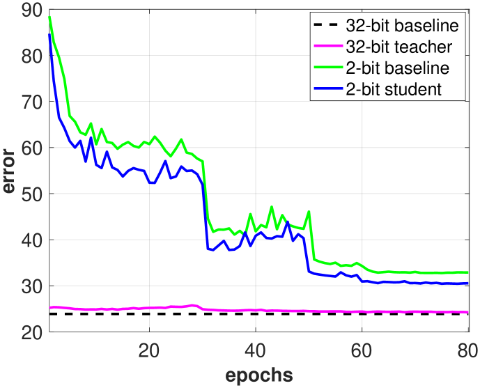
Figure 6: Student is learnt from scratch while teacher is fine-tuned. PreResNet-50 is used here.

4.3.3 Learning from the fixed teacher

In this section, we fix the pretrained teacher network and only fine-tune the student network. This is the scheme used by [19] to train their student network. The training details for the student network are the same as those described in Sec. 4.3.1.

From Table VII, we can observe that the improvement is relatively lower than that with jointly updated teachers in Table V. This proves that directly transferring the knowledge from the fixed pretrained teacher may not be optimal or not be suitable for quantization. Both $M_{\rm{low}}$ and $M_{\rm{full}}$ should be jointly optimized to adapt to each other.

However, this scheme has an advantage that one can pre-compute and store the guidance signals and access them during training $M_{\rm{low}}$, which can save the forward and backward pass computations w.r.t.  $M_{\rm{full}}$. For better understanding, we further show the convergence curves for AlexNet* on ImageNet in Figure 7.

TABLE VII: The accuracy of the quantized PreResNet using the fixed full-precision teacher.

Precision		PreResNet-18 Baseline	PreResNet-18 with PreResNet-18	PreResNet-34 Baseline	PreResNet-34 with PreResNet-34
4W, 4A	Top-1%	69.81	70.15	73.57	73.97
	Top-5%	89.07	89.48	91.35	91.72
2W, 2A	Top-1%	64.51	65.09	69.31	69.96
	Top-5%	85.85	86.44	88.92	89.51

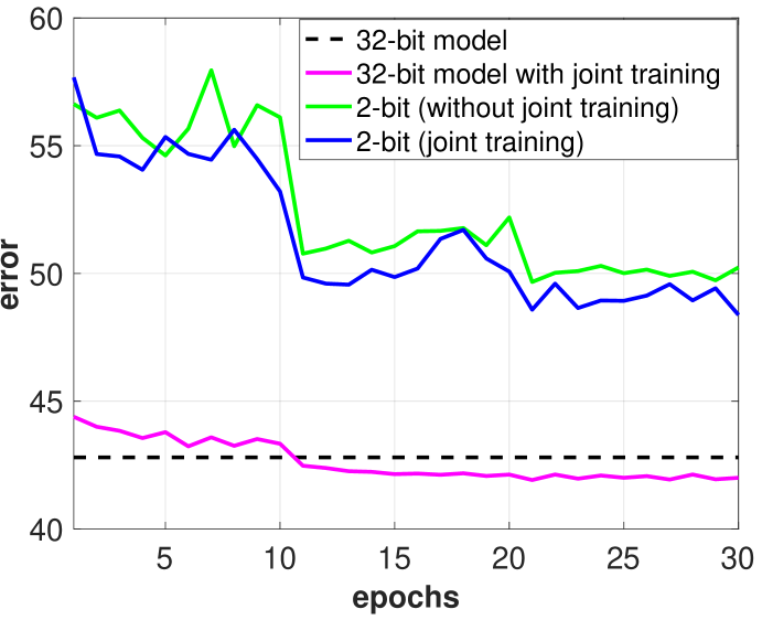
Figure 7: Joint training vs.  fixed teacher using AlexNet* on ImageNet.

4.3.4 Ablation study on guidance signals

In this part, we further explore the effect of different distillation guidance signals as introduced in Sec. 3.4. The results are reported in Table VIII. We observe that integrating both posterior-based and attention-based distillation strategies achieve the best result, performing better than using them separately.

TABLE VIII: Abalation study on the guidance signals with ResNet-50 on ImageNet.

Precision		ResNet-50 Baseline	ResNet-50 posterior	ResNet-50 attention transfer	ResNet-50 joint
2W, 2A	Top-1%	70.19	71.40	71.51	71.96
	Top-5%	89.15	90.04	90.17	90.63

4.3.5 Visualization

We further visualize and conduct more analysis on the experimental results in Figure 8. To explain why the proposed joint distillation strategy works better than the baseline, we illustrate the probability estimates assigned to Top-10 highest ranked classes obtained by a ResNet-18 on ImageNet trained by our joint distillation vs. an independently trained counterpart. This visualization is based on a randomly sampled mini-batch of 256. From Figure 8, we have two main observations. First, we see that the posterior distribution of our proposed joint KD fits the full-precision counterpart better, which expects to have more accurate predictions. Second, the posterior probability of the jointly updated full-precision teacher adapts better to the low-precision student than the fixed full-precision teacher. This observation justifies that, with our joint distillation strategy, the low-precision student and the full-precision teacher learn collaboratively and adapt to each other throughout the training process.

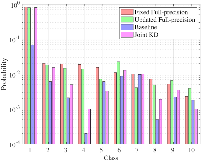
Figure 8: Mean posterior probability visualization.

4.4 Effect of quantizing all layers

In this part, we further explore the effect of quantizing the first convolution layer and the last classification layer to the final performance. We report the performance in Tables I, XI, XII and XIII. With “2W, 2A”, the performance of ResNet-50 beats ResNet-50* by a large margin. This shows that keeping the first and the last layer to high-precision is crucial to preserve the quantized model accuracy. Moreover, the proposed advanced training approaches improve the baseline significantly. For 2-bit precision, the gap between “ResNet-50* TS+PP+KD” and baseline* is 2.93% while “ResNet-50 TS+PP+KD” improves baseline by 2.21%. It further justifies the claim in Sec. 4.3.1 and Sec. 4.3.2 that the proposed training algorithms can be more effective when the model is more challenging to be optimized.

4.5 Combining different training strategies

TABLE IX: Accuracy (%) of ResNets on the ImageNet validation set using SP and KD. Experiments are repeated for 3 times and we report the results with mean and standard deviation.

Precision		ResNet-18 Baseline	ResNet-18 with ResNet-18	ResNet-34 Baseline	ResNet-34 with ResNet-34	ResNet-50 Baseline	ResNet-50 with ResNet-50
32W, 32A	Top-1%	69.75	-	73.21	-	75.64	-
	Top-5%	89.01	-	91.40	-	92.25	-
2W, 2A	Top-1%	64.67$\pm$0.04	66.07$\pm$0.06	68.17$\pm$0.05	70.33$\pm$0.05	70.19$\pm$0.04	73.25$\pm$0.06
	Top-5%	85.78$\pm$0.10	87.16$\pm$0.12	88.05$\pm$0.09	90.03$\pm$0.14	89.15$\pm$0.08	91.60$\pm$0.15

TABLE X: Accuracy (%) of PreResNets on the ImageNet validation set with SP and KD. Experiments are repeated for 3 times and we report the results with mean and standard deviation.

Precision		PreResNet-18 Baseline	PreResNet-18 with ResNet-18	PreResNet-34 Baseline	PreResNet-34 with PreResNet-34	PreResNet-50 Baseline	PreResNet-50 with PreResNet-50
32W, 32A	Top-1%	69.95	-	73.53	-	76.11	-
	Top-5%	89.21	-	91.30	-	92.81	-
2W, 2A	Top-1%	64.51$\pm$0.05	66.17$\pm$0.07	69.31$\pm$0.05	70.65$\pm$0.06	71.20$\pm$0.04	72.96$\pm$0.08
	Top-5%	85.85$\pm$0.10	87.14$\pm$0.13	88.92$\pm$0.11	89.72$\pm$0.16	90.18$\pm$0.10	91.31$\pm$0.14

TABLE XI: Accuracy (%) of ResNet-50 and ResNet-50* on the ImageNet with TS, PP and KD.

Precision		Baseline*	ResNet-50* TS + PP+ KD	Baseline	ResNet-50 TS + PP + KD
32W, 32A	Top-1%	75.64	-	-	-
	Top-5%	92.25	-	-	-
4W, 4A	Top-1%	74.30	75.78	74.50	75.85
	Top-5%	91.16	92.08	91.46	92.27
2W, 2A	Top-1%	67.69	70.62	70.19	72.40
	Top-5%	84.71	88.07	89.15	90.65

TABLE XII: Accuracy (%) of AlexNet* on the CIFAR-100 with SP and KD.

Precision		AlexNet* Baseline	AlexNet* SP + KD
32W, 32A	Top-1%	65.42	-
	Top-5%	88.31	-
2W, 2A	Top-1%	63.89	65.23
	Top-5%	87.58	88.44

TABLE XIII: Accuracy (%) of AlexNet* on the ImageNet with TS, PP and KD.

Precision		AlexNet* Baseline	AlexNet* TS + KD	AlexNet* TS + PP + KD
32W, 32A	Top-1%	57.22	-	-
	Top-5%	80.32	-	-
4W, 4A	Top-1%	56.80	57.92	58.21
	Top-5%	80.01	80.99	81.28
2W, 2A	Top-1%	48.79	51.38	51.96
	Top-5%	72.24	75.60	76.53

Finally, we come to our complete approach by combining TS, PP, SP and KD. We first combine TS, PP with KD and the results are shown in Tables XI and XIII. Moreover, we also combine the one-stage SP strategy with KD and the full results are reported in Tables IX, X and XII.

We observe that the proposed approaches can benefit from each other and further improve the performance on all settings. For instance, with “2W, 2A” in Table IX, we find a 3.06% relative gap between the baseline on ResNet-50. Even with the basic quantizer in DoReFa-Net, the difference in Top-1 error is only 2.39%. This strongly justifies that the proposed joint knowledge distillation and the stochastic precision are general training approaches for improving low-bit neural networks.

5 Conclusion

In this paper, we have proposed three novel approaches to solve the optimization problem for quantizing the network with both low-precision weights and activations. Firstly, we have proposed the progressive quantization approach which includes two schemes. Specifically, we have proposed a two-stage training scheme, where we use the real-valued activations as an intermediate step. We have also observed that continuously quantizing from high-precision to low-precision is also beneficial to the final performance. Moreover, we have proposed a stochastic precision strategy to significantly reduce the training complexity of progressive quantization while still improving the performance.

Furthermore, we have presented to improve the accuracy of low-precision networks with knowledge distillation. In particular, to better take advantage of the knowledge from the full-precision model, we have proposed to jointly learn the low-precision model and its full-precision counterpart. We have explored various distillation schemes and all observed improvements over the baseline. Finally, we have combined the three training approaches to further boost the performance. We have conducted extensive experiments to justify the effectiveness of the proposed approaches on the image classification task.

Bohan Zhuang is a Lecturer at Monash University, Australia. He received his PhD degree from The University of Adelaide.

Mingkui Tan is a Professor at South China University of Technology, China.

Jing Liu is a PhD student at Monash University.

Lingqiao Liu is a Senior Lecturer at The University of Adelaide.

Ian Reid is a Professor at The University of Adelaide.

Chunhua Shen is an Adjunct Professor at Monash University.

References

- [1] A. Krizhevsky, I. Sutskever, and G. E. Hinton, “Imagenet classification with deep convolutional neural networks,” in Proc. Adv. Neural Inf. Process. Syst., 2012, pp. 1097–1105.
- [2] K. Simonyan and A. Zisserman, “Very deep convolutional networks for large-scale image recognition,” in Proc. Int. Conf. Learn. Repren., 2015.
- [3] K. He, X. Zhang, S. Ren, and J. Sun, “Deep residual learning for image recognition,” in Proc. IEEE Conf. Comp. Vis. Patt. Recogn., 2016, pp. 770–778.
- [4] Z. Zhuang, M. Tan, B. Zhuang, J. Liu, Y. Guo, Q. Wu, J. Huang, and J. Zhu, “Discrimination-aware channel pruning for deep neural networks,” in Proc. Adv. Neural Inf. Process. Syst., 2018, pp. 875–886.
- [5] Y. He, X. Zhang, and J. Sun, “Channel pruning for accelerating very deep neural networks,” in Proc. IEEE Int. Conf. Comp. Vis., vol. 2, 2017, p. 6.
- [6] H. Li, A. Kadav, I. Durdanovic, H. Samet, and H. P. Graf, “Pruning filters for efficient convnets,” in Proc. Adv. Neural Inf. Process. Syst., 2017.
- [7] Y.-D. Kim, E. Park, S. Yoo, T. Choi, L. Yang, and D. Shin, “Compression of deep convolutional neural networks for fast and low power mobile applications,” arXiv preprint arXiv:1511.06530, 2015.
- [8] X. Zhang, J. Zou, K. He, and J. Sun, “Accelerating very deep convolutional networks for classification and detection,” IEEE Trans. Pattern Anal. Mach. Intell., vol. 38, no. 10, pp. 1943–1955, 2016.
- [9] A. Zhou, A. Yao, Y. Guo, L. Xu, and Y. Chen, “Incremental network quantization: Towards lossless cnns with low-precision weights,” in Proc. Int. Conf. Learn. Repren., 2017.
- [10] M. Courbariaux, Y. Bengio, and J.-P. David, “Binaryconnect: Training deep neural networks with binary weights during propagations,” in Proc. Adv. Neural Inf. Process. Syst., 2015, pp. 3123–3131.
- [11] C. Zhu, S. Han, H. Mao, and W. J. Dally, “Trained ternary quantization,” in Proc. Int. Conf. Learn. Repren., 2017.
- [12] S. Zhou, Y. Wu, Z. Ni, X. Zhou, H. Wen, and Y. Zou, “Dorefa-net: Training low bitwidth convolutional neural networks with low bitwidth gradients,” arXiv preprint arXiv:1606.06160, 2016.
- [13] Z. Guo, X. Zhang, H. Mu, W. Heng, Z. Liu, Y. Wei, and J. Sun, “Single path one-shot neural architecture search with uniform sampling,” arXiv preprint arXiv:1904.00420, 2019.
- [14] A. G. Howard, M. Zhu, B. Chen, D. Kalenichenko, W. Wang, T. Weyand, M. Andreetto, and H. Adam, “Mobilenets: Efficient convolutional neural networks for mobile vision applications,” arXiv preprint arXiv:1704.04861, 2017.
- [15] X. Zhang, X. Zhou, M. Lin, and J. Sun, “Shufflenet: An extremely efficient convolutional neural network for mobile devices,” in Proc. IEEE Conf. Comp. Vis. Patt. Recogn., 2018, pp. 6848–6856.
- [16] N. Srivastava, G. Hinton, A. Krizhevsky, I. Sutskever, and R. Salakhutdinov, “Dropout: a simple way to prevent neural networks from overfitting,” J. Mach. Learn. Res., vol. 15, no. 1, pp. 1929–1958, 2014.
- [17] G. Huang, Y. Sun, Z. Liu, D. Sedra, and K. Q. Weinberger, “Deep networks with stochastic depth,” in Proc. Eur. Conf. Comp. Vis. Workshops, 2016, pp. 646–661.
- [18] A. Romero, N. Ballas, S. E. Kahou, A. Chassang, C. Gatta, and Y. Bengio, “Fitnets: Hints for thin deep nets,” Proc. Int. Conf. Learn. Repren., 2015.
- [19] G. Hinton, O. Vinyals, and J. Dean, “Distilling the knowledge in a neural network,” in Proc. Adv. Neural Inf. Process. Syst. Workshops, 2014.
- [20] E. Parisotto, J. L. Ba, and R. Salakhutdinov, “Actor-mimic: Deep multitask and transfer reinforcement learning,” Proc. Int. Conf. Learn. Repren., 2016.
- [21] S. Zagoruyko and N. Komodakis, “Paying more attention to attention: Improving the performance of convolutional neural networks via attention transfer,” in Proc. Int. Conf. Learn. Repren., 2017.
- [22] J. Ba and R. Caruana, “Do deep nets really need to be deep?” in Proc. Adv. Neural Inf. Process. Syst., 2014, pp. 2654–2662.
- [23] B. Zhuang, C. Shen, M. Tan, L. Liu, and I. Reid, “Towards effective low-bitwidth convolutional neural networks,” in Proc. IEEE Conf. Comp. Vis. Patt. Recogn., 2018.
- [24] M. Rastegari, V. Ordonez, J. Redmon, and A. Farhadi, “Xnor-net: Imagenet classification using binary convolutional neural networks,” in Proc. Eur. Conf. Comp. Vis. Workshops, 2016, pp. 525–542.
- [25] I. Hubara, M. Courbariaux, D. Soudry, R. El-Yaniv, and Y. Bengio, “Binarized neural networks,” in Proc. Adv. Neural Inf. Process. Syst., 2016, pp. 4107–4115.
- [26] J. Bethge, M. Bornstein, A. Loy, H. Yang, and C. Meinel, “Training competitive binary neural networks from scratch,” arXiv preprint arXiv:1812.01965, 2018.
- [27] J. Bethge, H. Yang, C. Bartz, and C. Meinel, “Learning to train a binary neural network,” arXiv preprint arXiv:1809.10463, 2018.
- [28] W. Tang, G. Hua, and L. Wang, “How to train a compact binary neural network with high accuracy?” in Proc. Twenty-Eighth AAAI Conf. on Arti. Intel., 2017, pp. 2625–2631.
- [29] Y. Guo, A. Yao, H. Zhao, and Y. Chen, “Network sketching: Exploiting binary structure in deep cnns,” in Proc. IEEE Conf. Comp. Vis. Patt. Recogn., 2017, pp. 5955–5963.
- [30] Z. Liu, B. Wu, W. Luo, X. Yang, W. Liu, and K.-T. Cheng, “Bi-real net: Enhancing the performance of 1-bit cnns with improved representational capability and advanced training algorithm,” in Proc. Eur. Conf. Comp. Vis. Workshops, 2018.
- [31] J. Choi, Z. Wang, S. Venkataramani, P. I.-J. Chuang, V. Srinivasan, and K. Gopalakrishnan, “Pact: Parameterized clipping activation for quantized neural networks,” arXiv preprint arXiv:1805.06085, 2018.
- [32] S. K. Esser, J. L. McKinstry, D. Bablani, R. Appuswamy, and D. S. Modha, “Learned step size quantization,” in Proc. Int. Conf. Learn. Repren., 2020.
- [33] B. Zhuang, C. Shen, M. Tan, L. Liu, and I. Reid, “Strutured binary neural network for accurate image classification and semantic segmentation,” in Proc. IEEE Conf. Comp. Vis. Patt. Recogn., 2019.
- [34] X. Lin, C. Zhao, and W. Pan, “Towards accurate binary convolutional neural network,” in Proc. Adv. Neural Inf. Process. Syst., 2017, pp. 344–352.
- [35] Z. Cai, X. He, J. Sun, and N. Vasconcelos, “Deep learning with low precision by half-wave gaussian quantization,” in Proc. IEEE Conf. Comp. Vis. Patt. Recogn., 2017, pp. 5918–5926.
- [36] D. Zhang, J. Yang, D. Ye, and G. Hua, “Lq-nets: Learned quantization for highly accurate and compact deep neural networks,” in Proc. Eur. Conf. Comp. Vis. Workshops, 2018.
- [37] S. Jung, C. Son, S. Lee, J. Son, J.-J. Han, Y. Kwak, S. J. Hwang, and C. Choi, “Learning to quantize deep networks by optimizing quantization intervals with task loss,” in Proc. IEEE Conf. Comp. Vis. Patt. Recogn., 2019, pp. 4350–4359.
- [38] Y. Bengio, N. Léonard, and A. Courville, “Estimating or propagating gradients through stochastic neurons for conditional computation,” arXiv preprint arXiv:1308.3432, 2013.
- [39] L. Hou and J. T. Kwok, “Loss-aware weight quantization of deep networks,” in Proc. Int. Conf. Learn. Repren., 2018.
- [40] R. Ding, T.-W. Chin, Z. Liu, and D. Marculescu, “Regularizing activation distribution for training binarized deep networks,” in Proc. IEEE Conf. Comp. Vis. Patt. Recogn., 2019, pp. 11 408–11 417.
- [41] Y. Choi, M. El-Khamy, and J. Lee, “Learning low precision deep neural networks through regularization,” ArXiv, vol. abs/1809.00095, 2018.
- [42] Y. Bai, Y.-X. Wang, and E. Liberty, “Proxquant: Quantized neural networks via proximal operators,” in Proc. Int. Conf. Learn. Repren., 2019.
- [43] E. Park, J. Ahn, and S. Yoo, “Weighted-entropy-based quantization for deep neural networks,” in Proc. IEEE Conf. Comp. Vis. Patt. Recogn., 2017, pp. 5456–5464.
- [44] A. Polino, R. Pascanu, and D. Alistarh, “Model compression via distillation and quantization,” in Proc. Int. Conf. Learn. Repren., 2018.
- [45] C. Louizos, M. Reisser, T. Blankevoort, E. Gavves, and M. Welling, “Relaxed quantization for discretized neural networks,” in Proc. Int. Conf. Learn. Repren., 2019.
- [46] A. Ignatov, R. Timofte, W. Chou, K. Wang, M. Wu, T. Hartley, and L. Van Gool, “Ai benchmark: Running deep neural networks on android smartphones,” in Proc. Eur. Conf. Comp. Vis., 2018.
- [47] H. Yang, M. Fritzsche, C. Bartz, and C. Meinel, “Bmxnet: An open-source binary neural network implementation based on mxnet,” in Proc. of the ACM Int. Conf. on Multimedia. ACM, 2017, pp. 1209–1212.
- [48] Y. Umuroglu, N. J. Fraser, G. Gambardella, M. Blott, P. Leong, M. Jahre, and K. Vissers, “Finn: A framework for fast, scalable binarized neural network inference,” in Proceedings of the 2017 ACM/SIGDA International Symposium on Field-Programmable Gate Arrays. ACM, 2017, pp. 65–74.
- [49] B. Jacob, S. Kligys, B. Chen, M. Zhu, M. Tang, A. Howard, H. Adam, and D. Kalenichenko, “Quantization and training of neural networks for efficient integer-arithmetic-only inference,” in Proc. IEEE Conf. Comp. Vis. Patt. Recogn., 2018.
- [50] F. N. Iandola, S. Han, M. W. Moskewicz, K. Ashraf, W. J. Dally, and K. Keutzer, “Squeezenet: Alexnet-level accuracy with 50x fewer parameters and¡ 0.5 mb model size,” arXiv preprint arXiv:1602.07360, 2016.
- [51] F. Chollet, “Xception: Deep learning with depthwise separable convolutions,” in Proc. IEEE Conf. Comp. Vis. Patt. Recogn., 2017, pp. 1251–1258.
- [52] B. Zoph and Q. V. Le, “Neural architecture search with reinforcement learning,” in Proc. Int. Conf. Learn. Repren., 2017.
- [53] H. Pham, M. Y. Guan, B. Zoph, Q. V. Le, and J. Dean, “Efficient neural architecture search via parameter sharing,” in Proc. Int. Conf. Mach. Learn., 2018.
- [54] B. Zoph, V. Vasudevan, J. Shlens, and Q. V. Le, “Learning transferable architectures for scalable image recognition,” in Proc. IEEE Conf. Comp. Vis. Patt. Recogn., 2018.
- [55] C. Liu, B. Zoph, J. Shlens, W. Hua, L.-J. Li, L. Fei-Fei, A. Yuille, J. Huang, and K. Murphy, “Progressive neural architecture search,” in Proc. Eur. Conf. Comp. Vis. Workshops, 2018.
- [56] E. Real, A. Aggarwal, Y. Huang, and Q. V. Le, “Regularized evolution for image classifier architecture search,” in Proceedings of the aaai conference on artificial intelligence, vol. 33, 2019, pp. 4780–4789.
- [57] H. Liu, K. Simonyan, and Y. Yang, “Darts: Differentiable architecture search,” in Proc. Int. Conf. Learn. Repren., 2019.
- [58] H. Cai, L. Zhu, and S. Han, “Proxylessnas: Direct neural architecture search on target task and hardware,” in Proc. Int. Conf. Learn. Repren., 2019.
- [59] R. Yu, A. Li, C.-F. Chen, J.-H. Lai, V. I. Morariu, X. Han, M. Gao, C.-Y. Lin, and L. S. Davis, “Nisp: Pruning networks using neuron importance score propagation,” in Proc. IEEE Conf. Comp. Vis. Patt. Recogn., 2018, pp. 9194–9203.
- [60] A. Ashok, N. Rhinehart, F. Beainy, and K. M. Kitani, “N2n learning: Network to network compression via policy gradient reinforcement learning,” in Proc. Int. Conf. Learn. Repren., 2018.
- [61] Y. He, J. Lin, Z. Liu, H. Wang, L.-J. Li, and S. Han, “Amc: Automl for model compression and acceleration on mobile devices,” in Proc. Eur. Conf. Comp. Vis. Workshops, 2018.
- [62] F. Tung and G. Mori, “Clip-q: Deep network compression learning by in-parallel pruning-quantization,” in Proc. IEEE Conf. Comp. Vis. Patt. Recogn., 2018, pp. 7873–7882.
- [63] X. Dong and Y. Yang, “Network pruning via transformable architecture search,” in Proc. Adv. Neural Inf. Process. Syst., 2019, pp. 760–771.
- [64] B. Zhang, L. Wang, Z. Wang, Y. Qiao, and H. Wang, “Real-time action recognition with enhanced motion vector cnns,” in Proc. IEEE Conf. Comp. Vis. Patt. Recogn., 2016, pp. 2718–2726.
- [65] G. Chen, W. Choi, X. Yu, T. Han, and M. Chandraker, “Learning efficient object detection models with knowledge distillation,” in Proc. Adv. Neural Inf. Process. Syst., 2017, pp. 742–751.
- [66] Y. Wei, X. Pan, H. Qin, W. Ouyang, and J. Yan, “Quantization mimic: Towards very tiny cnn for object detection,” in Proc. Eur. Conf. Comp. Vis. Workshops, 2018, pp. 267–283.
- [67] T. He, C. Shen, Z. Tian, D. Gong, C. Sun, and Y. Yan, “Knowledge adaptation for efficient semantic segmentation,” arXiv preprint arXiv:1903.04688, 2019.
- [68] A. Mishra and D. Marr, “Apprentice: Using knowledge distillation techniques to improve low-precision network accuracy,” in Proc. Int. Conf. Learn. Repren., 2018.
- [69] I. J. Goodfellow, D. Warde-Farley, M. Mirza, A. Courville, and Y. Bengio, “Maxout networks,” in Proc. Int. Conf. Mach. Learn., 2013.
- [70] L. Wan, M. Zeiler, S. Zhang, Y. Le Cun, and R. Fergus, “Regularization of neural networks using dropconnect,” in Proc. Int. Conf. Mach. Learn., 2013, pp. 1058–1066.
- [71] L. N. Smith, E. M. Hand, and T. Doster, “Gradual dropin of layers to train very deep neural networks,” in Proc. IEEE Conf. Comp. Vis. Patt. Recogn., 2016, pp. 4763–4771.
- [72] Y. Dong, R. Ni, J. Li, Y. Chen, J. Zhu, and H. Su, “Learning accurate low-bit deep neural networks with stochastic quantization,” in Proc. Brit. Mach. Vis. Conf., 2017.
- [73] J. Yu, L. Yang, N. Xu, J. Yang, and T. Huang, “Slimmable neural networks,” 2019.
- [74] J. Yu and T. S. Huang, “Universally slimmable networks and improved training techniques,” in Proc. IEEE Int. Conf. Comp. Vis., 2019, pp. 1803–1811.
- [75] A. Krizhevsky and G. Hinton, “Learning multiple layers of features from tiny images,” 2009.
- [76] O. Russakovsky, J. Deng, H. Su, J. Krause, S. Satheesh, S. Ma, Z. Huang, A. Karpathy, A. Khosla, M. Bernstein et al., “Imagenet large scale visual recognition challenge,” Int. J. Comp. Vis., vol. 115, no. 3, pp. 211–252, 2015.
- [77] K. He, X. Zhang, S. Ren, and J. Sun, “Identity mappings in deep residual networks,” in Proc. Eur. Conf. Comp. Vis. Workshops, 2016, pp. 630–645.
- [78] E. Park, D. Kim, S. Yoo, and P. Vajda, “Precision highway for ultra low-precision quantization,” arXiv preprint arXiv:1812.09818, 2018.