Form factors of $V^{\prime}\to V^{\prime\prime}$ transition within the light-front quark models

Abstract

In this paper, we calculate the matrix element and form factors of vector-to-vector ($V^{\prime}\to V^{\prime\prime}$) transition within the standard light-front (SLF) and covariant light-front (CLF) quark models (QMs), and investigate the self-consistency and Lorentz covariance of the CLF QM within two types of correspondences between the manifest covariant Bethe-Salpeter approach and the LF approach. The zero-mode and valence contributions to the form factors of $V^{\prime}\to V^{\prime\prime}$ transition in the CLF QM and their relation to the SLF results are analyzed, and the main conclusions obtained via the decay constants of vector and axial-vector mesons and the form factors of $P\to V$ transition in the previous works are confirmed again. Furthermore, we present our numerical predictions for the form factors of $c\to(q,s)$ ($q=u,d$) induced $D^{*}\to(K^{*}\,,\rho)$, $D^{*}_{s}\to(\phi\,,K^{*})$, $J/\Psi\to(D^{*}_{s}\,,D^{*})$, $B^{*}_{c}\to(B^{*}_{s}\,,B^{*})$ transitions and $b\to(q,s,c)$ induced $B^{*}\to(D^{*}\,,K^{*}\,,\rho)$, $B^{*}_{s}\to(D^{*}_{s}\,,\phi\,,K^{*})$, $B^{*}_{c}\to(J/\Psi\,,D^{*}_{s}\,,D^{*})$, $\Upsilon(1S)\to(B_{c}^{*}\,,B_{s}^{*}\,,B^{*})$ transitions, which can be applied further to the relevant phenomenological studies of meson decays.

1 Introduction

The mesonic transition form factors are important ingredients in the study of weak and electromagnetic decays of mesons. There are many approaches for evaluating these nonperturbative quantities, for instance, Wirbel-Stech-Bauer model [1], lattice calculations [2], vector meson dominance model [3, 4], perturbative QCD with some nonperturbative inputs [5, 6], QCD sum rules [7, 8] and light-front quark models (LF QMs) [9, 10, 11, 12, 13]. In this paper, we will calculate the form factors of $V^{\prime}\to V^{\prime\prime}$ transition ($V^{\prime}$ and $V^{\prime\prime}$ denote vector mesons) within the standard and the covariant light-front approaches.

The standard light-front quark model (SLF QM) proposed by Terentev and Berestetsky [9, 10] is a relativistic quark model based on the LF formalism [14] and LF quantization of QCD [15]. It provides a conceptually simple and phenomenologically feasible framework for the determination of nonperturbative quantities. However, the matrix element evaluated in this approach lacks manifest Lorentz covariance and the zero-mode contributions can not be determined explicitly. In order to fill these gaps, many efforts have been made in the past years [11, 12, 13, 16, 17, 18, 19]. In Ref. [12], a method based on the covariant LF framework is developed to identify and separate the $\omega$-dependent spurious contributions, where $\omega$ is the light-like four-vector used to define light-front by $\omega\cdot x=0$ and the $\omega$-dependent contributions may violate the covariance. With such an approach, the $\omega$-independent physical contributions can be well determined, while the effects of zero-mode are not fully considered. In Ref. [13], a basically different technique is developed by Jaus to deal with the covariance and zero-mode problems with the help of a manifestly covariant Bethe-Saltpeter (BS) approach as a guide to the calculation. In such a covariant light-front quark model (CLF QM), the zero-mode contributions can be well determined, and the result of the matrix element is expected to be covariant because the spurious contributions can be eliminated by the inclusion of zero-mode contributions [13].

The SLF and CLF QMs have been widely used for the determination of nonperturbative quantities, such as form factor, decay constant and distribution amplitude, as well as the other features, of hadrons, which are further applied to phenomenological researches [20, 21, 24, 25, 26, 27, 28, 29, 30, 31, 32, 33, 34, 35, 36, 37, 38, 39, 40, 22, 23, 41, 42, 43, 44, 45, 46, 47, 48, 49, 50, 51, 52, 53, 54, 55, 56, 57, 58, 59, 60, 61, 62, 63, 64, 65, 66, 67, 68, 71, 72, 73, 69, 70, 74, 75]. For the weak decays, the form factors of $P\to(P\,,V)$ transitions have been calculated within the SLF and the CLF QMs in Refs. [20, 21, 22] and Refs. [13, 69, 70, 71], respectively; besides, the form factors of $P\to(S\,,A\,,T)$ transitions are studied within the CLF QM [70, 71]. In addition, the SLF approach is also used to evaluate the form factors of $\text{baryon}\to\text{baryon}$ processes with help of diquark picture [76, 78, 77, 79, 80, 81]. However, the form factors of $V^{\prime}\to V^{\prime\prime}$ transition have not been fully investigated. With the rapid development of particle physics experiment, some weak decays of vector mesons are hopeful to be observed by LHC and SuperKEKB/Belle-II experiments et al. in the future due to the high luminosity [82, 83, 84]. The theoretical evaluation of the form factors of $V^{\prime}\to V^{\prime\prime}$ transition can provide some useful references and essential inputs for the relevant phenomenological studies. In Ref. [69], the angular condition for $\langle V^{\prime\prime}|\gamma^{\mu}|V^{\prime}\rangle$ are studied, but only the electromagnetic transition form factors ($V^{\prime}=V^{\prime\prime}=\rho$) are obtained. In this paper, the form factors related to the current matrix elements, $\langle V^{\prime\prime}|\gamma^{\mu}|V^{\prime}\rangle$ and $\langle V^{\prime\prime}|\gamma^{\mu}\gamma_{5}|V^{\prime}\rangle$, will be calculated within the SLF and CLF QMs, and moreover, the self-consistency and covariance of CLF QM and the effects of zero-mode will be analyzed in detail.

The manifest covariance is a remarkable feature of the CLF QM relative to the SLF QM [13]. However, it should be noted that although the main $\omega$ dependences are associated with the $C$ functions and can be eliminated by the zero-mode contributions, there are still some residual $\omega$ dependences due to the nonvanishing spurious contributions associated with $B$ functions², which are unfortunately nonzero within the traditional correspondence scheme between the covariant BS model and the LF QM (named as type-I scheme [85]), and therefore violate the strict covariance of CLF results [13, 69, 86, 87]. Besides, the self-consistency is another challenge to the CLF QM. For instance, the authors of Ref. [70] find that the CLF results for $f_{V}$ obtained respectively via longitudinal ($\lambda=0$) and transverse ($\lambda=\pm$) polarization states are inconsistent with each other, $[f_{V}]_{\rm CLF}^{\lambda=0}\neq[f_{V}]_{\rm CLF}^{\lambda=\pm}$, because the former receives an additional contribution characterized by the $B_{1}^{(2)}$ function.

In order to recover the self-consistency of CLF QM, the authors of Ref. [85] present a modified correspondence between the covariant BS approach and the LF approach (named as type-II scheme [85]), which requires an additional $M\to M_{0}$ replacement relative to the traditional type-I correspondence scheme. Within this modified correspondence scheme, $[f_{V}]_{\rm CLF}^{\lambda=0}\dot{=}[f_{V}]_{\rm CLF}^{\lambda=\pm}$ [85] is obtained. In our previous works [86, 87], the problems of self-consistency and covariance are studied via $f_{P,V,A}$ and form factors of $P\to(P,V)$ transitions. It is found that such two problems have the same origin, and can be resolved simultaneously by employing type-II correspondence scheme because the contributions associated with $B_{1}^{(2)}$ and $B_{3}^{(3)}$ functions vanish numerically [86, 87]. Moreover, it is also found that  [85, 86, 87]

$$[{\cal Q}]_{\rm SLF}=[{\cal Q}]_{\rm val.}\doteq[{\cal Q}]_{\rm CLF},$$ (1)

where ${\cal Q}$ denotes $f_{P,V,A}$ and form factors of $P\to(P,V)$ transitions, the subscript “val.” denotes the valence contribution in the CLF QM, and the symbol “$\doteq$” denotes that the two quantities are equal to each other numerically. The form factors of $V^{\prime}\to V^{\prime\prime}$ transition involves much more $B$ functions and thus may present much stricter test on the CLF QM, as well as above-mentioned findings. In this paper, these issues will be studied in detail.

Our paper is organized as follows. In sections 2 and 3, we would like to review briefly the SLF and the CLF QMs, respectively, for convenience of discussion, and then present our theoretical results for the form factors of $V^{\prime}\to V^{\prime\prime}$ transition. In section 4, the self-consistency and covariance of CLF results are discussed in detail, and the zero-mode and the valence contribution in the CLF QM and their relations to the SLF results are analyzed. After that, we present our numerical results for some $c\to(q,s)$ and $b\to(q,s,c)$ ($q=u,d$) induced transitions. Finally, our summary is made in section 5.

2 Theoretical results in the SLF QM

2.1 General formalism

In this section, in order to clarify the convention and notation used in this paper, we would like to review briefly the framework of SLF QM. One may refer to, for instance, Refs. [20, 21] for details. The form factors of $V^{\prime}\to V^{\prime\prime}$ transition can be defined as [88]

$$\langle V^{\prime\prime}(\epsilon^{\prime\prime},p^{\prime\prime})|\bar{q}^{\prime\prime}_{1}\gamma_{\mu}q^{\prime}_{1}|V^{\prime}(\epsilon^{\prime},p^{\prime})\rangle= -(\epsilon^{\prime}\cdot\epsilon^{\prime\prime*})\Big{[}P_{\mu}\,V_{1}(q^{2})-q_{\mu}\,V_{2}(q^{2})\Big{]}$$

$$+\frac{(\epsilon^{\prime}\cdot q)(\epsilon^{\prime\prime*}\cdot q)}{M^{\prime 2}-M^{\prime\prime 2}}\bigg{[}\Big{(}P^{\nu}-\frac{M^{\prime 2}-M^{\prime\prime 2}}{q^{2}}q^{\nu}\Big{)}\,V_{3}(q^{2})$$

$$+\frac{M^{\prime 2}-M^{\prime\prime 2}}{q^{2}}q^{\nu}\,V_{4}(q^{2})\bigg{]}$$

$$-(\epsilon^{\prime}\cdot q)\,\epsilon^{\prime\prime*}_{\mu}\,V_{5}(q^{2})+(\epsilon^{\prime\prime*}\cdot q)\,\epsilon^{\prime}_{\mu}\,V_{6}(q^{2})\,,$$ (2)

$$\langle V^{\prime\prime}(\epsilon^{\prime\prime},p^{\prime\prime})|\bar{q}^{\prime\prime}_{1}\gamma_{\mu}\gamma_{5}q^{\prime}_{1}|V^{\prime}(\epsilon^{\prime},p^{\prime})\rangle= -i\varepsilon_{\mu\nu\alpha\beta}\epsilon^{\prime\alpha}\epsilon^{\prime\prime*\beta}\bigg{[}\Big{(}P^{\nu}-\frac{M^{\prime 2}-M^{\prime\prime 2}}{q^{2}}q^{\nu}\Big{)}\,A_{1}(q^{2})$$

$$+\frac{M^{\prime 2}-M^{\prime\prime 2}}{q^{2}}q^{\nu}\,A_{2}(q^{2})\bigg{]}$$

$$-\frac{i\,\varepsilon_{\mu\nu\alpha\beta}P^{\alpha}q^{\beta}}{M^{\prime 2}-M^{\prime\prime 2}}\,\Big{[}\epsilon^{\prime\prime*}\cdot q\,\epsilon^{\prime\nu}A_{3}(q^{2})-\epsilon^{\prime}\cdot q\,\epsilon^{\prime\prime*\nu}A_{4}(q^{2})\Big{]}$$

where, $P=p^{\prime}+p^{\prime\prime}$, $q=p^{\prime}-p^{\prime\prime}$ and $\varepsilon_{0123}=-1$. The main work of LF approach is to evaluate the current matrix element,

$${\cal B}\equiv\langle V^{\prime\prime}(\epsilon^{\prime\prime},p^{\prime\prime})|\bar{q}^{\prime\prime}_{1}(k_{1}^{\prime\prime})\Gamma q^{\prime}_{1}(k_{1}^{\prime})|V^{\prime}(\epsilon^{\prime},p^{\prime})\rangle\,,\qquad\Gamma=\gamma_{\mu}\,,\gamma_{\mu}\gamma_{5}\,,$$ (4)

which will be further used to extract the form factors.

In the framework of SLF QM, a meson bound-state consisting a quark $q_{1}$ and antiquark $\bar{q}_{2}$ with a total momentum $p$ can be written as

$$|M(p)\rangle=\sum_{h_{1},h_{2}}\int\frac{{\rm d}^{3}\tilde{k}_{1}}{(2\pi)^{3}2\sqrt{k_{1}^{+}}}\frac{{\rm d}^{3}\tilde{k}_{2}}{(2\pi)^{3}2\sqrt{k_{2}^{+}}}(2\pi)^{3}\delta^{3}({\tilde{p}-\tilde{k}_{1}-\tilde{k}_{2}})\Psi_{h_{1},h_{2}}(\tilde{k}_{1},\tilde{k}_{2})|q_{1}({k}_{1},h_{1})\rangle|\bar{q}_{2}({k}_{2},h_{2})\rangle\,,$$ (5)

where, $\tilde{p}=(p^{+},\mathbf{p_{\bot}})$ and $\tilde{k}_{1,2}=(k_{1,2}^{+},\mathbf{k}_{1,2\bot})$ are the on-mass-shell LF momenta, $\Psi_{h_{1},h_{2}}(\tilde{k}_{1},\tilde{k}_{2})$ is the momentum-space wavefunction (WF), and the one particle state is defined as $|q_{1}({k}_{1},h_{1})\rangle=\sqrt{2k_{1}^{+}}\,b_{h1}^{\dagger}(k_{1})|0\rangle$ and $|\bar{q}_{2}({k}_{2},h_{2})\rangle=\sqrt{2k_{2}^{+}}\,d_{h2}^{\dagger}(k_{2})|0\rangle$. The momenta of $q_{1}$ and $\bar{q}_{2}$ can be written in terms of the internal LF relative momentum variables $(x,{\mathbf{k}_{\bot}})$ as

$$k_{1}^{+}=xp^{+}\,,\quad\,\mathbf{k}_{1\bot}=x\mathbf{p}_{\bot}+\mathbf{k}_{\bot}\,,\qquad k_{2}^{+}=\bar{x}p^{+}\,,\quad\,\mathbf{k}_{2\bot}=\bar{x}\mathbf{p}_{\bot}-\mathbf{k}_{\bot}\,,$$ (6)

where, $\bar{x}=1-x$, $\mathbf{k}_{\bot}=(k^{x}\,,k^{y})$ and $\mathbf{p}_{\bot}=(p^{x}\,,p^{y})$.

The momentum-space WF in Eq. (5) satisfies the normalization condition and can be expressed as

$$\Psi_{h_{1},h_{2}}(x,\mathbf{k}_{\bot})=S_{h_{1},h_{2}}(x,\mathbf{k}_{\bot})\psi(x,\mathbf{k}_{\bot})\,,$$ (7)

where, $\psi(x,\mathbf{k}_{\bot})$ is the radial WF and responsible for describing the momentum distribution of the constituent quarks in the bound-state; $S_{h_{1},h_{2}}(x,\mathbf{k}_{\bot})$ is the spin-orbital WF and responsible for constructing a state of definite spin $(S,S_{z})$ out of the LF helicity $(h_{1},h_{2})$ eigenstates. For the former, we adopt the Gaussian type WF

$$\psi_{s}(x,\mathbf{k}_{\bot})=4\frac{\pi^{\frac{3}{4}}}{\beta^{\frac{3}{2}}}\sqrt{\frac{\partial k_{z}}{\partial x}}\exp\left[-\frac{k_{z}^{2}+\mathbf{k}_{\bot}^{2}}{2\beta^{2}}\right]\,,$$ (8)

where, $k_{z}$ is the relative momentum in $z$-direction and can be written as

$$k_{z}=(x-\frac{1}{2})M_{0}+\frac{m_{2}^{2}-m_{1}^{2}}{2M_{0}}\,,$$ (9)

with the invariant mass $M_{0}^{2}=\frac{m_{1}^{2}+\mathbf{k}_{\bot}^{2}}{x}+\frac{m_{2}^{2}+\mathbf{k}_{\bot}^{2}}{\bar{x}}$. Besides the Gaussian type WF, there are some other choices, which will be discussed later. The spin-orbital WF, $S_{h_{1},h_{2}}(x,\mathbf{k}_{\bot})$, can be obtained by the interaction-independent Melosh transformation. It is convenient to use its covariant form, which can be further reduced by using the equation of motion on spinors and finally written as [21, 70]

$$S_{h_{1},h_{2}}=\frac{\bar{u}(k_{1},h_{1})\Gamma^{\prime}v(k_{2},h_{2})}{\sqrt{2}\hat{M}_{0}}\,,$$ (10)

where, $\hat{M}_{0}^{2}=M_{0}^{2}-(m_{1}-m_{2})^{2}$. For the vector state, one shall take

$$\Gamma^{\prime}_{V}=-\not\!\hat{\epsilon}+\frac{\hat{\epsilon}\cdot(k_{1}-k_{2})}{D_{V,{\rm LF}}}\,,\quad D_{V,{\rm LF}}=M_{0}+m_{1}+m_{2}\,,$$ (11)

where,

$$\hat{\epsilon}^{\mu}_{\lambda=0}= \frac{1}{M_{0}}\left(p^{+},\frac{-M_{0}^{2}+\mathbf{p}_{\bot}^{2}}{p^{+}},\mathbf{p}_{\bot}\right)\,,$$ (12)

$$\hat{\epsilon}^{\mu}_{\lambda=\pm}= \left(0,\frac{2}{p^{+}}\boldsymbol{\epsilon}_{\bot}\cdot\mathbf{p}_{\bot},\boldsymbol{\epsilon}_{\bot}\right)\,,\quad\boldsymbol{\epsilon}_{\bot}\equiv\mp\frac{(1,\pm i)}{\sqrt{2}}\,.$$ (13)

In practice, for the $V^{\prime}(p^{\prime})\to V^{\prime\prime}(p^{\prime\prime})$ transition, we shall take the convenient Drell-Yan-West frame, $q^{+}=0$, where $q\equiv p^{\prime}-p^{\prime\prime}=k_{1}^{\prime}-k_{1}^{\prime\prime}$ is the momentum transfer. In addition, we also take a Lorentz frame where $\mathbf{p}_{\bot}^{\prime}=0$ for convenience of calculation. In this frame, the momenta of constituent quarks in initial and final states are written as

$$\tilde{k}_{1}^{\prime}=(xp^{\prime+},\mathbf{k}_{\bot}^{\prime})\,,\quad\tilde{k}_{1}^{\prime\prime}=(xp^{\prime+},x\mathbf{p}_{\bot}^{\prime\prime}+\mathbf{k}_{\bot}^{\prime\prime})\,,\quad\tilde{k}_{2}=(\bar{x}p^{\prime+},-\mathbf{k}_{\bot}^{\prime})=(\bar{x}p^{\prime+},\bar{x}\mathbf{p}_{\bot}^{\prime\prime}-\mathbf{k}_{\bot}^{\prime\prime})\,,$$ (14)

where, $\mathbf{p}_{\bot}^{\prime\prime}=-\mathbf{q}_{\bot}$ and $\mathbf{k}_{\bot}^{\prime\prime}=\mathbf{k}_{\bot}^{\prime}-\bar{x}\mathbf{q}_{\bot}$.

Finally, equipping Eq. (4) with the formulas given above and making some simplifications, we obtain

$${\cal B}_{\rm SLF}=\sum_{h^{\prime}_{1},h^{\prime\prime}_{1},h_{2}}\int\frac{{\rm d}x\,{\rm d}^{2}{\mathbf{k}_{\bot}^{\prime}}}{(2\pi)^{3}\,2x}{\psi^{\prime\prime}}^{*}(x,\mathbf{k}_{\bot}^{\prime\prime}){\psi^{\prime}}(x,\mathbf{k}_{\bot}^{\prime})S^{\prime\prime\dagger}_{h^{\prime\prime}_{1},h_{2}}(x,\mathbf{k}_{\bot}^{\prime\prime})\,C_{h^{\prime\prime}_{1},h^{\prime}_{1}}(x,\mathbf{k}_{\bot}^{\prime},\mathbf{k}_{\bot}^{\prime\prime})\,S^{\prime}_{h^{\prime}_{1},h_{2}}(x,\mathbf{k}_{\bot}^{\prime})\,,$$ (15)

where $C_{h^{\prime\prime}_{1},h^{\prime}_{1}}(x,\mathbf{k}_{\bot}^{\prime},\mathbf{k}_{\bot}^{\prime\prime})\equiv\bar{u}_{h^{\prime\prime}_{1}}(x,\mathbf{k}_{\bot}^{\prime\prime})\Gamma u_{h^{\prime}_{1}}(x,\mathbf{k}_{\bot}^{\prime})$.

2.2 Theoretical results

Using the formulas given in the last subsection, one can obtain the expression of ${\cal B}_{\rm SLF}^{\mu}$ for the $V^{\prime}\to V^{\prime\prime}$ transition. In the SLF QM, in order to extract the form factors, one has to take explicit $\mu$, $\lambda^{\prime}$ and $\lambda^{\prime\prime}$. In this work, for convenience of calculation, we take the strategy as follows: (i) We take $\mu=+$ firstly and then use ${\cal B}_{\rm SLF}^{+}$ with $(\lambda^{\prime},\lambda^{\prime\prime})=(-,+)$, $(+,+)$, $(+,0)$ and $(0,+)$ to extract $V_{3}$, $V_{1}$, $V_{5}$ and $V_{6}$, respectively; (ii) We multiply both sides of Eq. (2.1) by $\epsilon^{\prime\mu*}$, and then use ${\cal B}_{\rm SLF}\cdot\epsilon^{\prime*}$ with $(\lambda^{\prime},\lambda^{\prime\prime})=(-,+)$ and $(+,+)$ to extract $V_{4}$ and $V_{2}$, respectively. (iii) For $A_{1}$, $A_{2}$, $A_{3}$ and $A_{4}$, we take $\lambda^{\prime}=\lambda^{\prime\prime}=\pm$, and multiply both sides of Eq. (2.1) by $q^{\mu}$, $P^{\mu}$, $\epsilon^{\prime\prime\mu*}$ and $\epsilon^{\prime\mu}$, respectively. After some derivations and simplifications, we finally obtain the SLF results for the form factors of $V^{\prime}\to V^{\prime\prime}$ transition written as

$$[{\cal F}(q^{2})]_{\rm SLF}=\int\frac{{\rm d}x\,{\rm d}^{2}{\bf k_{\bot}^{\prime}}}{(2\pi)^{3}\,2x}\frac{{\psi^{\prime\prime}}^{*}(x,{\bf k^{\prime\prime}_{\bot}})\,{\psi^{\prime}}(x,{\bf k_{\bot}^{\prime}})}{2\hat{M}^{\prime}_{0}\hat{M}^{\prime\prime}_{0}}\,{\cal\widetilde{F}}^{\rm SLF}(x,{\bf k}_{\bot}^{\prime},q^{2})\,,$$ (16)

where, ${\cal F}$ denotes $V_{1-6}$ and $A_{1-4}$, and the integrands are

$$\widetilde{V}_{1}^{\rm SLF}= 2\bigg{\{}4x\frac{({\bf k}_{\bot}^{\prime}\cdot{\bf q}_{\bot})^{2}}{{\bf q}_{\bot}^{2}}+\frac{(\bar{x}-x)^{2}}{\bar{x}}{\bf k}_{\bot}^{\prime 2}-{\bf k}_{\bot}^{\prime}\cdot{\bf q}_{\bot}+\frac{1}{\bar{x}}(\bar{x}m^{\prime}_{1}+xm_{2})(\bar{x}m^{\prime\prime}_{1}+xm_{2})$$

$$-\frac{4}{D^{\prime}_{V,{\rm LF}}}\Big{[}{\bf k}_{\bot}^{\prime 2}-\frac{({\bf k}_{\bot}^{\prime}\cdot{\bf q}_{\bot})^{2}}{{\bf q}_{\bot}^{2}}\Big{]}\Big{[}(\bar{x}-x)m^{\prime}_{1}-m^{\prime\prime}_{1}-2xm_{2}\Big{]}$$

$$+\frac{4}{D^{\prime\prime}_{V,{\rm LF}}}\Big{[}{\bf k}_{\bot}^{\prime 2}-\frac{({\bf k}_{\bot}^{\prime}\cdot{\bf q}_{\bot})^{2}}{{\bf q}_{\bot}^{2}}\Big{]}\Big{[}m^{\prime}_{1}-(\bar{x}-x)m^{\prime\prime}_{1}+2xm_{2}\Big{]}$$

$$+\frac{8}{\bar{x}D^{\prime}_{V,{\rm LF}}D^{\prime\prime}_{V,{\rm LF}}}\Big{[}{\bf k}_{\bot}^{\prime 2}-\frac{({\bf k}_{\bot}^{\prime}\cdot{\bf q}_{\bot})^{2}}{{\bf q}_{\bot}^{2}}\Big{]}\Big{[}{\bf k}_{\bot}^{\prime}\cdot{\bf k}_{\bot}^{\prime\prime}+(\bar{x}m^{\prime}_{1}-xm_{2})(\bar{x}m_{1}^{\prime\prime}-xm_{2})\Big{]}\bigg{\}}\,,$$ (17)

$$\widetilde{V}_{2}^{\rm{SLF}}= \frac{4}{x\bar{x}}\bigg{\{}-\frac{{\bf k}_{\bot}^{\prime}\cdot{\bf q}_{\bot}}{{\bf q}_{\bot}^{2}}(\bar{x}m^{\prime}_{1}+xm_{2})^{2}-(1-2x\bar{x})\frac{{\bf k}_{\bot}^{\prime\prime}\cdot{\bf q}_{\bot}}{{\bf q}_{\bot}^{2}}{\bf k}_{\bot}^{\prime 2}+x^{2}{\bf k}_{\bot}^{\prime}\cdot{\bf k}_{\bot}^{\prime\prime}$$

$$+(\bar{x}m^{\prime}_{1}+xm_{2})(\bar{x}^{2}m^{\prime}_{1}+x\bar{x}m^{\prime\prime}_{1}+xm_{2})$$

$$-\frac{x\bar{x}}{D^{\prime}_{V,{\rm LF}}}\Big{[}2\frac{{\bf k}_{\bot}^{\prime}\cdot{\bf q}_{\bot}}{{\bf q}_{\bot}^{2}}{\bf k}_{\bot}^{\prime 2}(m^{\prime}_{1}+m_{2})+{{\bf k}_{\bot}^{\prime}\cdot{\bf q}_{\bot}}(\bar{x}m^{\prime}_{1}-xm_{2})-{\bf k}_{\bot}^{\prime 2}\big{(}(1+2\bar{x})m^{\prime}_{1}+m^{\prime\prime}_{1}+2\bar{x}m_{2}\big{)}\Big{]}$$

$$+\frac{1}{D^{\prime\prime}_{V,{\rm LF}}}\frac{{\bf k}_{\bot}^{\prime\prime}\cdot{\bf q}_{\bot}}{{\bf q}_{\bot}^{2}}\Big{[}2\bar{x}(\bar{x}m^{\prime}_{1}+xm_{2}){\bf k^{\prime}_{\bot}\cdot q_{\bot}}-{\bf k}_{\bot}^{\prime 2}\big{(}m^{\prime}_{1}-(1-2x\bar{x})m^{\prime\prime}_{1}+2x\bar{x}m_{2}\big{)}$$

$$-(\bar{x}m^{\prime}_{1}+xm_{2})\big{(}(m^{\prime}_{1}-m^{\prime\prime}_{1})(xm_{2}-\bar{x}m^{\prime\prime}_{1})-\bar{x}q^{2}\big{)}\Big{]}$$

$$-\frac{1}{D^{\prime}_{V,{\rm LF}}D^{\prime\prime}_{V,{\rm LF}}}\Big{[}\frac{{\bf k}_{\bot}^{\prime\prime}\cdot{\bf q}_{\bot}}{{\bf q}_{\bot}^{2}}{\bf k}_{\bot}^{\prime 2}\Big{(}2{\bf k^{\prime}_{\bot}\cdot\bar{k}^{\prime\prime}_{\bot}}-\bar{x}q^{2}+(\bar{x}m^{\prime}_{1}-xm_{2})^{2}+(\bar{x}m^{\prime\prime}_{1}-xm_{2})^{2}$$

$$+x\bar{x}(m^{\prime}_{1}-m^{\prime\prime}_{1})^{2}\Big{)}-{\bf k}^{\prime}_{\bot}\cdot{\bf k}^{\prime\prime}_{\bot}\Big{(}{\bf k}_{\bot}^{\prime 2}+(xm_{2}-\bar{x}m^{\prime}_{1})^{2}\Big{)}\Big{]}\bigg{\}}$$

$$-\widetilde{V}_{1}^{\rm{SLF}}(x,{\bf k^{\prime}_{\bot}},q^{2})-\widetilde{V}_{6}^{\rm{SLF}}(x,{\bf k^{\prime}_{\bot}},q^{2})+\frac{q^{2}}{2(M^{\prime 2}-M^{\prime\prime 2})}\Big{[}\widetilde{V}_{3}^{\rm{SLF}}(x,{\bf k^{\prime}_{\bot}},q^{2})+\widetilde{V}_{4}^{\rm{SLF}}(x,{\bf k^{\prime}_{\bot}},q^{2})\Big{]}\,,$$ (18)

$$\widetilde{V}_{3}^{\textup{\scriptsize SLF}}= \frac{4(M^{\prime 2}-M^{\prime\prime 2})}{q^{2}}\bigg{\{}-2x\Big{[}{\bf k}_{\bot}^{\prime 2}+\bar{x}{\bf k}_{\bot}^{\prime}\cdot{\bf q}_{\bot}-2\frac{({\bf k}_{\bot}^{\prime}\cdot{\bf q}_{\bot})^{2}}{{\bf q}_{\bot}^{2}}\Big{]}$$

$$-\frac{1}{D^{\prime}_{V,{\rm LF}}}\Big{[}{\bf k}_{\bot}^{\prime}\cdot{\bf q}_{\bot}(\bar{x}-x)(\bar{x}m^{\prime}_{1}-xm_{2})+\Big{(}{\bf k}_{\bot}^{\prime 2}-2\frac{({\bf k}_{\bot}^{\prime}\cdot{\bf q}_{\bot})^{2}}{{\bf q}_{\bot}^{2}}\Big{)}\Big{(}(\bar{x}-x)m^{\prime}_{1}-m^{\prime\prime}_{1}-2xm_{2}\Big{)}\Big{]}$$

$$+\frac{1}{D^{\prime\prime}_{V,{\rm LF}}}\Big{[}\bar{x}(\bar{x}m^{\prime}_{1}+xm_{2})q^{2}+{\bf k^{\prime}_{\bot}\cdot q_{\bot}}\Big{(}2\bar{x}m^{\prime}_{1}-\bar{x}(\bar{x}-x)m^{\prime\prime}_{1}+x(2\bar{x}+1)m_{2}\Big{)}$$

$$+\Big{(}{\bf k}_{\bot}^{\prime 2}-2\frac{({\bf k}_{\bot}^{\prime}\cdot{\bf q}_{\bot})^{2}}{{\bf q}_{\bot}^{2}}\Big{)}\Big{(}m^{\prime}_{1}-(\bar{x}-x)m^{\prime\prime}_{1}+2xm_{2}\Big{)}\Big{]}$$

$$+\frac{2}{\bar{x}D^{\prime}_{V,{\rm LF}}D^{\prime\prime}_{V,{\rm LF}}}\Big{[}{\bf k}_{\bot}^{\prime 2}+\bar{x}{\bf k}_{\bot}^{\prime}\cdot{\bf q}_{\bot}-2\frac{({\bf k}_{\bot}^{\prime}\cdot{\bf q}_{\bot})^{2}}{{\bf q}_{\bot}^{2}}\Big{]}\Big{[}{\bf k}_{\bot}^{\prime}\cdot{\bf k}_{\bot}^{\prime\prime}+(\bar{x}m^{\prime}_{1}-xm_{2})(\bar{x}m^{\prime\prime}_{1}-xm_{2})\Big{]}\bigg{\}}\,,$$ (19)

$$\widetilde{V}_{4}^{\rm SLF}= -8\bigg{\{}(1-2x){\bf k}^{\prime 2}_{\bot}+\frac{2({\bf k^{\prime}_{\bot}\cdot q_{\bot}})^{2}}{{\bf q}_{\bot}^{2}}-\frac{\bf k^{\prime}_{\bot}\cdot q_{\bot}}{{\bf q}_{\bot}^{2}}\Big{[}2{\bf k}^{\prime 2}_{\bot}-\bar{x}q^{2}+(m^{\prime}_{1}-m^{\prime\prime}_{1})^{2}\Big{]}$$

$$+(m^{\prime}_{1}-m^{\prime\prime}_{1})(\bar{x}m^{\prime}_{1}+xm_{2})$$

$$+\frac{1}{x\bar{x}D^{\prime}_{V,{\rm LF}}}\Big{[}2\bar{x}(\bar{x}m^{\prime}_{1}-xm_{2})\frac{({\bf k^{\prime}_{\bot}\cdot q_{\bot}})^{2}}{{\bf q}_{\bot}^{2}}-\bar{x}{\bf k}^{\prime 2}_{\bot}\big{(}x(\bar{x}-x)m^{\prime}_{1}+xm^{\prime\prime}_{1}-2x^{2}m_{2}\big{)}$$

$$+\frac{\bf k^{\prime}_{\bot}\cdot q_{\bot}}{{\bf q}_{\bot}^{2}}(\bar{x}m^{\prime}_{1}-xm_{2})\big{(}(m^{\prime}_{1}-m^{\prime\prime}_{1})(\bar{x}m^{\prime}_{1}+xm_{2})+\bar{x}^{2}q^{2}\big{)}$$

$$+\frac{\bf k^{\prime}_{\bot}\cdot q_{\bot}}{{\bf q}_{\bot}^{2}}{\bf k}^{\prime 2}_{\bot}\big{(}(2x\bar{x}-1)m^{\prime}_{1}+m^{\prime\prime}_{1}+2x\bar{x}m_{2}\big{)}\Big{]}$$

$$-\frac{1}{x\bar{x}D^{\prime\prime}_{V,{\rm LF}}}\frac{\bf k^{\prime\prime}_{\bot}\cdot q_{\bot}}{{\bf q}_{\bot}^{2}}\Big{[}2\bar{x}(\bar{x}m^{\prime}_{1}+xm_{2}){\bf k^{\prime}_{\bot}\cdot q_{\bot}}-{\bf k}_{\bot}^{\prime 2}(m^{\prime}_{1}-m^{\prime\prime}_{1}+2x\bar{x}m^{\prime\prime}_{1}+2x\bar{x}m_{2})$$

$$-(\bar{x}m^{\prime}_{1}+xm_{2})\big{(}(m^{\prime}_{1}-m^{\prime\prime}_{1})(xm_{2}-\bar{x}m^{\prime\prime}_{1})-\bar{x}q^{2}\big{)}\Big{]}$$

$$+\frac{1}{x\bar{x}D^{\prime}_{V,{\rm LF}}D^{\prime\prime}_{V,{\rm LF}}}\Big{[}\frac{\bf k^{\prime\prime}_{\bot}\cdot q_{\bot}}{{\bf q}_{\bot}^{2}}{\bf k}_{\bot}^{\prime 2}\Big{(}2{\bf k^{\prime}_{\bot}\cdot k^{\prime\prime}_{\bot}}-\bar{x}(1-2x)q^{2}+(\bar{x}m^{\prime}_{1}-xm_{2})^{2}+(\bar{x}m^{\prime\prime}_{1}-xm_{2})^{2}$$

$$+x\bar{x}(m^{\prime}_{1}-m^{\prime\prime}_{1})^{2}\Big{)}-\Big{(}\frac{2({\bf k^{\prime}_{\bot}\cdot q_{\bot}})^{2}}{{\bf q}_{\bot}^{2}}-{\bf k}_{\bot}^{\prime 2}-\bar{x}{\bf k^{\prime}_{\bot}\cdot q_{\bot}}\Big{)}\big{(}{\bf k}_{\bot}^{\prime 2}+(xm_{2}-\bar{x}m^{\prime}_{1})^{2}\big{)}\Big{]}\bigg{\}}$$

$$+\left(1+\frac{q^{2}}{M^{\prime 2}-M^{\prime\prime 2}}\right)\widetilde{V}_{3}^{\rm{SLF}}(x,{\bf k^{\prime}_{\bot}},q^{2})+2\left[\widetilde{V}_{5}^{\rm{SLF}}(x,{\bf k^{\prime}_{\bot}},q^{2})-\widetilde{V}_{6}^{\rm{SLF}}(x,{\bf k^{\prime}_{\bot}},q^{2})\right]\,,$$ (20)

$$\widetilde{V}_{5}^{\rm{SLF}}= \frac{4M^{\prime\prime}}{M_{0}^{\prime\prime}}\bigg{\{}2(x-\bar{x})\frac{({\bf k}_{\bot}^{\prime}\cdot{\bf q}_{\bot})^{2}}{{\bf q}_{\bot}^{2}}-(m^{\prime\prime}_{1}-m_{2})(\bar{x}m^{\prime}_{1}+xm_{2})$$

$$-\frac{{\bf k}_{\bot}^{\prime}\cdot{\bf q}_{\bot}}{{\bf q}_{\bot}^{2}}\Big{[}(x-\bar{x})(x{M^{\prime\prime}_{0}}^{2}-\bar{x}q^{2})+\frac{x-\bar{x}}{\bar{x}}{\bf k}_{\bot}^{\prime 2}+\frac{x}{\bar{x}}m_{2}^{2}-m^{\prime}_{1}m^{\prime\prime}_{1}+(m^{\prime}_{1}-m^{\prime\prime}_{1})m_{2}\Big{]}$$

$$+\frac{2}{\bar{x}D^{\prime}_{V,{\rm LF}}}\frac{{\bf k}_{\bot}^{\prime}\cdot{\bf q}_{\bot}}{{\bf q}_{\bot}^{2}}\Big{[}(xm_{2}-\bar{x}m^{\prime}_{1})(m^{\prime\prime}_{1}m_{2}+\bar{x}xM_{0}^{\prime\prime 2}-\bar{x}^{2}q^{2})$$

$$+{\bf k}^{\prime 2}_{\bot}\big{(}m^{\prime\prime}_{1}-\bar{x}m^{\prime}_{1}-\bar{x}m_{2}\big{)}+\bar{x}{\bf k^{\prime}_{\bot}\cdot q_{\bot}}\big{(}2\bar{x}m^{\prime}_{1}-m^{\prime\prime}_{1}+(\bar{x}-x)m_{2}\big{)}\Big{]}$$

$$-\frac{1}{x\bar{x}D^{\prime\prime}_{V,{\rm LF}}}\Big{[}\bar{x}m^{\prime}_{1}+xm_{2}-\frac{{\bf k}_{\bot}^{\prime}\cdot{\bf q}_{\bot}}{{\bf q}_{\bot}^{2}}\big{(}m^{\prime}_{1}+(x-\bar{x})m^{\prime\prime}_{1}+2xm_{2}\big{)}\Big{]}\Big{[}(x-\bar{x}){\bf k}_{\bot}^{\prime\prime 2}-\bar{x}^{2}m_{1}^{\prime\prime 2}+x^{2}m_{2}^{2}\Big{]}$$

$$+\frac{2}{x\bar{x}^{2}D^{\prime}_{V,{\rm LF}}D^{\prime\prime}_{V,{\rm LF}}}\frac{{\bf k}_{\bot}^{\prime}\cdot{\bf q}_{\bot}}{{\bf q}_{\bot}^{2}}\Big{[}{\bf k}_{\bot}^{\prime}\cdot{\bf k}_{\bot}^{\prime\prime}+(xm_{2}-\bar{x}m^{\prime}_{1})(xm_{2}-\bar{x}m^{\prime\prime}_{1})\Big{]}\Big{[}(x-\bar{x}){\bf k}_{\bot}^{\prime\prime 2}-\bar{x}^{2}m_{1}^{\prime\prime 2}+x^{2}m_{2}^{2}\Big{]}\bigg{\}}$$

$$+2\widetilde{V}_{1}^{\rm{SLF}}(x,{\bf k^{\prime}_{\bot}},q^{2})+\left(1-\frac{q^{2}}{M^{\prime 2}-M^{\prime\prime 2}}\right)\widetilde{V}_{3}^{\rm{SLF}}(x,{\bf k^{\prime}_{\bot}},q^{2})\,,$$ (21)

$$\widetilde{V}_{6}^{\rm{SLF}}= \frac{4M^{\prime}}{M_{0}^{\prime}}\bigg{\{}(\bar{x}-x)({\bf k}^{\prime 2}_{\bot}+x\bar{x}M_{0}^{\prime 2}+m^{\prime}_{1}m_{2})$$

$$+\frac{{\bf k}_{\bot}^{\prime}\cdot{\bf q}_{\bot}}{{\bf q}_{\bot}^{2}}\Big{[}x(x-\bar{x})M_{0}^{\prime 2}+\frac{x-\bar{x}}{\bar{x}}(m_{2}^{2}+{\bf k}^{\prime 2}_{\bot})-(m_{2}-m_{1}^{\prime})(m_{2}+m_{1}^{\prime\prime})\Big{]}$$

$$-\frac{1}{\bar{x}D^{\prime}_{V,{\rm LF}}}\big{(}m_{2}^{2}+{\bf k}^{\prime 2}_{\bot}-\bar{x}^{2}M_{0}^{\prime 2}\big{)}\Big{[}(x-\bar{x})(xm_{2}-\bar{x}m^{\prime}_{1})+\frac{{\bf k}_{\bot}^{\prime}\cdot{\bf q}_{\bot}}{{\bf q}_{\bot}^{2}}\big{(}m^{\prime\prime}_{1}+(x-\bar{x})m^{\prime}_{1}+2xm_{2})\big{)}\Big{]}$$

$$+\frac{2}{\bar{x}D^{\prime\prime}_{V,{\rm LF}}}\frac{{\bf k}_{\bot}^{\prime\prime}\cdot{\bf q}_{\bot}}{{\bf q}_{\bot}^{2}}\Big{[}(\bar{x}m^{\prime\prime}_{1}-xm_{2})(m^{\prime}_{1}m_{2}+x\bar{x}M_{0}^{\prime 2}+{\bf k}_{\bot}^{\prime 2})-{\bf k}_{\bot}^{\prime}\cdot{\bf k}_{\bot}^{\prime\prime}(m^{\prime}_{1}-m_{2})\Big{]}$$

$$+\frac{2}{\bar{x}^{2}D^{\prime}_{V,{\rm LF}}D^{\prime\prime}_{V,{\rm LF}}}\frac{{\bf k}_{\bot}^{\prime\prime}\cdot{\bf q}_{\bot}}{{\bf q}_{\bot}^{2}}(m_{2}^{2}+{\bf k}^{\prime 2}_{\bot}-\bar{x}^{2}M_{0}^{\prime 2})\Big{[}{\bf k}^{\prime 2}_{\bot}+\bar{x}{\bf k^{\prime}_{\bot}\cdot q}_{\bot}+(xm_{2}-\bar{x}m^{\prime}_{1})(xm_{2}-\bar{x}m^{\prime\prime}_{1})\Big{]}\bigg{\}}$$

$$+2\widetilde{V}_{1}^{\rm{SLF}}(x,{\bf k^{\prime}_{\bot}},q^{2})-\left(1-\frac{q^{2}}{M^{\prime 2}-M^{\prime\prime 2}}\right)\widetilde{V}_{3}^{\rm{SLF}}(x,{\bf k^{\prime}_{\bot}},q^{2})\,,$$ (22)

$$\widetilde{A}_{1}^{\rm{SLF}}= \frac{2}{x\bar{x}({M^{\prime}}^{2}-{M^{\prime\prime}}^{2})}\bigg{\{}(x-\bar{x}){\bf k}_{\bot}^{\prime}\cdot{\bf k}_{\bot}^{\prime\prime}\left[\bar{x}{\bf q}_{\bot}^{2}-2{\bf k_{\bot}^{\prime}\cdot q_{\bot}}+x({M^{\prime}}^{2}-{M^{\prime\prime}}^{2})\right]$$

$$+{\bf k^{\prime}_{\bot}\cdot q_{\bot}}\left(\bar{x}^{2}m_{1}^{\prime 2}+\bar{x}^{2}m_{1}^{\prime\prime 2}-2x^{2}m_{2}^{2}\right)+\bar{x}{\bf q}_{\bot}^{2}(-\bar{x}^{2}{m^{\prime}_{1}}^{2}+x^{2}m_{2}^{2})$$

$$+x(\bar{x}m^{\prime}_{1}+xm_{2})(\bar{x}m^{\prime\prime}_{1}+xm_{2})({M^{\prime}}^{2}-{M^{\prime\prime}}^{2})$$

$$-\frac{1}{D_{V,{\rm LF}}^{\prime}}\Big{[}2\bar{x}({\bf k_{\bot}^{\prime}\cdot q_{\bot}})^{2}(xm^{\prime\prime}_{1}+xm_{2}+xm^{\prime}_{1}-\bar{x}m^{\prime}_{1})$$

$$-x\bar{x}(m^{\prime}_{1}+m^{\prime\prime}_{1})({M^{\prime}}^{2}-{M^{\prime\prime}}^{2}-q^{2}){\bf k}_{\bot}^{\prime 2}-{\bf k^{\prime}_{\bot}\cdot q_{\bot}}{\bf k}_{\bot}^{\prime 2}(x-\bar{x})(m^{\prime}_{1}+m^{\prime\prime}_{1})$$

$$-{\bf k^{\prime}_{\bot}\cdot q_{\bot}}(\bar{x}m^{\prime}_{1}-xm_{2})\left((\bar{x}m^{\prime\prime}_{1}+xm_{2})(m^{\prime}_{1}+m^{\prime\prime}_{1})+\bar{x}^{2}{\bf q}_{\bot}^{2}+x\bar{x}({M^{\prime}}^{2}-{M^{\prime\prime}}^{2})\right)\Big{]}$$

$$-\frac{1}{D^{\prime\prime}_{V,{\rm LF}}}\Big{[}x\bar{x}(m^{\prime}_{1}+m^{\prime\prime}_{1})({M^{\prime}}^{2}-{M^{\prime\prime}}^{2}-q^{2}){\bf k^{\prime}_{\bot}\cdot k^{\prime\prime}_{\bot}}$$

$$-(x-\bar{x})(m^{\prime}_{1}+m^{\prime\prime}_{1}){\bf k^{\prime\prime}_{\bot}\cdot q_{\bot}}{\bf k}_{\bot}^{\prime 2}-\bar{x}(\bar{x}m^{\prime}_{1}+xm_{2}){\bf k^{\prime\prime}_{\bot}\cdot q_{\bot}}({\bf k}_{\bot}^{\prime}+{\bf k}_{\bot}^{\prime\prime})\cdot{\bf q}_{\bot}$$

$$-(\bar{x}m^{\prime}_{1}+xm_{2})\big{(}(m^{\prime}_{1}+m^{\prime\prime}_{1})(xm_{2}-\bar{x}m^{\prime\prime}_{1})-x\bar{x}({M^{\prime}}^{2}-{M^{\prime\prime}}^{2})\big{)}{\bf k^{\prime\prime}_{\bot}\cdot q_{\bot}}\Big{]}$$

$$-\frac{2\bar{x}^{2}}{D^{\prime}_{V,{\rm LF}}D^{\prime\prime}_{V,{\rm LF}}}\Big{[}{\bf k}_{\bot}^{\prime 2}{\bf q}_{\bot}^{2}-({\bf k^{\prime}_{\bot}\cdot q_{\bot}})^{2}\Big{]}\Big{[}{m^{\prime}_{1}}^{2}-{m^{\prime\prime}_{1}}^{2}-x(M^{\prime 2}-M^{\prime\prime 2})+{\bf(k^{\prime}_{\bot}+k^{\prime\prime}_{\bot})\cdot q_{\bot}}\Big{]}\bigg{\}}\,,$$ (23)

$$\widetilde{A}_{2}^{\rm{SLF}}= \frac{2\,q^{2}}{({M^{\prime}}^{2}-{M^{\prime\prime}}^{2})^{2}}\bigg{\{}\frac{{\bf k}_{\bot}^{\prime 2}}{x^{2}\bar{x}}\Big{[}2(\bar{x}-x){\bf k}_{\bot}^{\prime 2}+\bar{x}(2+x^{2}-5x\bar{x}){\bf q}_{\bot}^{2}+2\bar{x}^{2}({m^{\prime}_{1}}^{2}+{m^{\prime\prime}_{1}}^{2})$$

$$+2(xm^{\prime}_{1}+\bar{x}m_{2})(xm^{\prime\prime}_{1}+\bar{x}m_{2})-2(\bar{x}-x)m_{2}^{2}-x^{2}(x-\bar{x})({M^{\prime}}^{2}+{M^{\prime\prime}}^{2})\Big{]}$$

$$+\frac{\bf k^{\prime}_{\bot}\cdot q_{\bot}}{x^{2}}\Big{[}4(x-\bar{x}){\bf k}_{\bot}^{\prime 2}-2x{\bf k^{\prime}_{\bot}\cdot q_{\bot}}-x\bar{x}(\bar{x}-x)q^{2}+\bar{x}(3x-4)m_{1}^{\prime 2}+x\bar{x}{m^{\prime\prime}_{1}}^{2}$$

$$+4x^{2}m_{2}^{2}-4xm^{\prime}_{1}m_{2}-2x^{2}(m^{\prime}_{1}-m_{2})(m^{\prime\prime}_{1}-m_{2})+(x-\bar{x})\cdot x^{2}({M^{\prime}}^{2}+{M^{\prime\prime}}^{2})\Big{]}$$

$$-\frac{\bar{x}m^{\prime}_{1}+xm_{2}}{x^{2}\bar{x}}\Big{[}\bar{x}(x^{2}m_{2}+\bar{x}^{2}m_{1}^{\prime}+\bar{x}m_{1}^{\prime})q^{2}-2m^{\prime}_{1}m^{\prime\prime}_{1}(\bar{x}{m^{\prime\prime}_{1}}+xm_{2})$$

$$+x^{2}(\bar{x}m^{\prime\prime}_{1}+xm_{2})({M^{\prime}}^{2}+{M^{\prime\prime}}^{2})\Big{]}$$

$$+\frac{1}{x\bar{x}D^{\prime}_{V,{\rm LF}}}\Big{[}{\bf k}_{\bot}^{\prime 2}(m^{\prime}_{1}+m^{\prime\prime}_{1})\big{(}2{\bf k}_{\bot}^{\prime 2}+2m_{2}^{2}+2\bar{x}(m^{\prime}_{1}+m_{2})(m^{\prime\prime}_{1}-m_{2})-\bar{x}x({M^{\prime}}^{2}+{M^{\prime\prime}}^{2})\big{)}$$

$$+{\bf q}_{\bot}^{2}{\bf k}_{\bot}^{\prime 2}\,\bar{x}\big{(}(2\bar{x}-x)m^{\prime}_{1}+xm^{\prime\prime}_{1}+2(\bar{x}-x)m_{2}\big{)}+{\bf k}_{\bot}^{\prime}\cdot{\bf q}_{\bot}{\bf k}_{\bot}^{\prime 2}\big{(}(x-\bar{x})m^{\prime\prime}_{1}-(1+4\bar{x})m^{\prime}_{1}-2\bar{x}m_{2}\big{)}$$

$$+2\bar{x}(m^{\prime}_{1}-xm^{\prime\prime}_{1}+xm_{2})({\bf k}_{\bot}^{\prime}\cdot{\bf q}_{\bot})^{2}+{\bf k}_{\bot}^{\prime}\cdot{\bf q}_{\bot}(xm_{2}-\bar{x}m^{\prime}_{1})\big{(}(m^{\prime}_{1}+m^{\prime\prime}_{1})(\bar{x}m^{\prime\prime}_{1}+xm_{2})$$

$$-2m^{\prime}_{1}m_{2}-x\bar{x}({M^{\prime}}^{2}+{M^{\prime\prime}}^{2})\big{)}+{\bf k}_{\bot}^{\prime}\cdot{\bf q}_{\bot}{\bf q}_{\bot}^{2}\bar{x}^{2}(xm_{2}-\bar{x}m^{\prime}_{1})\Big{]}$$

$$+\frac{1}{x\bar{x}D^{\prime\prime}_{V,{\rm LF}}}\Big{[}\big{(}({\bf k^{\prime}_{\bot}\cdot q_{\bot}})^{2}-{\bf k}_{\bot}^{\prime 2}{\bf q}_{\bot}^{2}\big{)}\big{(}3\bar{x}^{2}m^{\prime}_{1}+\bar{x}(x-2\bar{x})m_{2}\big{)}+2{\bf k}_{\bot}^{\prime 2}{\bf k}_{\bot}^{\prime}\cdot{\bf k}_{\bot}^{\prime\prime}(m^{\prime}_{1}+m^{\prime\prime}_{1})$$

$$-2{\bf k^{\prime}_{\bot}\cdot q_{\bot}}{\bf k}_{\bot}^{\prime}\cdot{\bf k}_{\bot}^{\prime\prime}\bar{x}(m^{\prime}_{1}-m_{2})+\bar{x}\big{(}(2\bar{x}+1)m^{\prime}_{1}-xm_{1}^{\prime\prime}+(x-2)m_{2}\big{)}{\bf k}_{\bot}^{\prime}\cdot{\bf k}_{\bot}^{\prime\prime}{\bf q}_{\bot}^{2}$$

$$+{\bf k}_{\bot}^{\prime}\cdot{\bf k}_{\bot}^{\prime\prime}\big{(}2m_{2}^{2}+2\bar{x}(m^{\prime}_{1}-m_{2})(m^{\prime\prime}_{1}+m_{2})-x\bar{x}({M^{\prime}}^{2}+{M^{\prime\prime}}^{2})\big{)}(m^{\prime}_{1}+m^{\prime\prime}_{1})$$

$$+{\bf k}_{\bot}^{\prime\prime}\cdot{\bf q}_{\bot}{\bf k}_{\bot}^{\prime 2}\big{(}(x-\bar{x})(m^{\prime}_{1}+m^{\prime\prime}_{1})-2m^{\prime}_{1}\big{)}+({\bf k}_{\bot}^{\prime\prime}\cdot{\bf q}_{\bot})^{2}\bar{x}(\bar{x}m_{1}^{\prime}+xm_{2})$$

$$+{\bf k}_{\bot}^{\prime\prime}\cdot{\bf q}_{\bot}(\bar{x}m_{1}^{\prime}+xm_{2})\big{(}(m^{\prime}_{1}+m^{\prime\prime}_{1})(xm_{2}-\bar{x}m^{\prime\prime}_{1})-2m^{\prime}_{1}m_{2}+x\bar{x}({M^{\prime}}^{2}+{M^{\prime\prime}}^{2})\big{)}\Big{]}$$

$$+\frac{2}{xD^{\prime}_{V,{\rm LF}}D^{\prime\prime}_{V,{\rm LF}}}\Big{[}\big{(}({\bf k^{\prime}_{\bot}\cdot q_{\bot}})^{2}-{\bf k}_{\bot}^{\prime 2}{\bf q}_{\bot}^{2}\big{)}\big{(}{\bar{x}}^{2}q^{2}-2{\bf k^{\prime}_{\bot}\cdot k^{\prime\prime}_{\bot}}-\bar{x}({m^{\prime}_{1}}^{2}+{m^{\prime\prime}_{1}}^{2})-2xm_{2}^{2}$$

$$+x\bar{x}({M^{\prime}}^{2}+{M^{\prime\prime}}^{2})\big{)}\Big{]}\bigg{\}}+\widetilde{A}_{1}^{\rm{SLF}}(x,{\bf k^{\prime}_{\bot}},q^{2})\,,$$ (24)

$$\widetilde{A}_{3}^{\rm{SLF}}= \frac{4}{x\bar{x}}\bigg{\{}\frac{\bf k_{\bot}^{\prime\prime}\cdot q_{\bot}}{{\bf q}_{\bot}^{2}}\Big{[}(x-\bar{x}){\bf k}_{\bot}^{\prime 2}-\bar{x}^{2}m_{1}^{\prime 2}+x^{2}m_{2}^{2}\Big{]}-{\bf k_{\bot}^{\prime}\cdot k}_{\bot}^{\prime\prime}$$

$$+\frac{1}{D^{\prime\prime}_{V,{\rm LF}}}\Big{[}{\bf k_{\bot}^{\prime}\cdot k_{\bot}^{\prime\prime}}\big{(}(x-\bar{x})\bar{x}m^{\prime}_{1}+x\bar{x}m^{\prime\prime}_{1}-x\bar{x}m_{2}\big{)}+\bar{x}^{2}(\bar{x}m^{\prime}_{1}+xm_{2}){\bf k_{\bot}^{\prime\prime}\cdot q_{\bot}}$$

$$+\Big{(}{\bf k}_{\bot}^{\prime 2}+\bar{x}{\bf k^{\prime}_{\bot}\cdot q_{\bot}}-2\frac{({\bf k^{\prime}_{\bot}\cdot q_{\bot}})^{2}}{{\bf q}_{\bot}^{2}}\Big{)}\left(\bar{x}^{2}m^{\prime}_{1}+x\bar{x}m_{2}\right)-\frac{\bf k_{\bot}^{\prime\prime}\cdot q_{\bot}}{{\bf q}_{\bot}^{2}}{\bf k^{\prime 2}_{\bot}}(x-\bar{x})(m^{\prime}_{1}+m^{\prime\prime}_{1})$$

$$-\frac{\bf k_{\bot}^{\prime\prime}\cdot q_{\bot}}{{\bf q}_{\bot}^{2}}(\bar{x}m^{\prime}_{1}+xm_{2})(m^{\prime}_{1}+m^{\prime\prime}_{1})(xm_{2}-\bar{x}m^{\prime\prime}_{1})\Big{]}$$

$$+\frac{1}{D^{\prime}_{V,{\rm LF}}D^{\prime\prime}_{V,{\rm LF}}}\Big{[}\Big{(}{\bf k}_{\bot}^{\prime 2}-\frac{2({\bf k^{\prime}_{\bot}\cdot q_{\bot}})^{2}}{{\bf q}_{\bot}^{2}}\Big{)}\big{(}\bar{x}{\bf k}_{\bot}^{\prime 2}-x\bar{x}^{2}q^{2}\big{)}+\bar{x}({\bf k^{\prime}_{\bot}\cdot q_{\bot}}){\bf k}_{\bot}^{\prime 2}$$

$$-{\bf k^{\prime}_{\bot}\cdot k^{\prime\prime}_{\bot}}(x{\bf k}_{\bot}^{\prime 2}-\bar{x}^{2}{m^{\prime}_{1}}^{2}+x^{2}m_{2}^{2})-\frac{\bf k^{\prime\prime}_{\bot}\cdot q_{\bot}}{{\bf q}_{\bot}^{2}}{\bf k}_{\bot}^{\prime 2}(\bar{x}{m^{\prime}_{1}}^{2}-\bar{x}{m^{\prime\prime}_{1}}^{2}+\bar{x}^{2}q^{2})\Big{]}\bigg{\}}\,,$$ (25)

$$\widetilde{A}_{4}^{\rm{SLF}}= \frac{4}{x\bar{x}}\bigg{\{}\bar{x}{\bf k}_{\bot}^{\prime 2}-\frac{\bf k^{\prime}_{\bot}\cdot q_{\bot}}{{\bf q}_{\bot}^{2}}\Big{[}(\bar{x}-x)({\bf k}_{\bot}^{\prime 2}-2\bar{x}{\bf k^{\prime}_{\bot}\cdot q_{\bot}})+\bar{x}^{2}{m^{\prime\prime}_{1}}^{2}-x^{2}m_{2}^{2}-\bar{x}^{3}q^{2}\Big{]}$$

$$+\frac{1}{D^{\prime}_{V,{\rm LF}}}\Big{[}2\frac{({\bf k^{\prime}_{\bot}\cdot q_{\bot}})^{2}}{{\bf q}_{\bot}^{2}}\left((x\bar{x}-\bar{x}^{2})m^{\prime}_{1}+x\bar{x}m^{\prime\prime}_{1}+x\bar{x}m_{2}\right)-x\bar{x}(m^{\prime}_{1}+m^{\prime\prime}_{1}){\bf k}_{\bot}^{\prime 2}$$

$$-\bar{x}^{2}(xm_{2}-\bar{x}m^{\prime}_{1}){\bf k^{\prime}_{\bot}\cdot q_{\bot}}+\frac{\bf k^{\prime}_{\bot}\cdot q_{\bot}}{{\bf q}_{\bot}^{2}}{\bf k}_{\bot}^{\prime 2}(\bar{x}-x)(m^{\prime}_{1}+m^{\prime\prime}_{1})$$

$$-\frac{\bf k^{\prime}_{\bot}\cdot q_{\bot}}{{\bf q}_{\bot}^{2}}(xm_{2}-\bar{x}m^{\prime}_{1})(m^{\prime}_{1}+m^{\prime\prime}_{1})(xm_{2}+\bar{x}m^{\prime\prime}_{1})\Big{]}$$

$$+\frac{1}{D^{\prime}_{V,{\rm LF}}D^{\prime\prime}_{V,{\rm LF}}}\Big{[}2\bar{x}\frac{({\bf k^{\prime}_{\bot}\cdot q_{\bot}})^{2}}{{\bf q}_{\bot}^{2}}{\bf k^{\prime}_{\bot}\cdot k^{\prime\prime}_{\bot}}+{\bf k^{\prime}_{\bot}\cdot k^{\prime\prime}_{\bot}}\big{(}(x-\bar{x}){\bf k}_{\bot}^{\prime 2}-\bar{x}^{2}{m^{\prime}_{1}}^{2}+x^{2}m_{2}^{2}\big{)}$$

$$+\Big{(}\bar{x}{\bf k}_{\bot}^{\prime 2}+\frac{\bf k^{\prime}_{\bot}\cdot q_{\bot}}{{\bf q}_{\bot}^{2}}{\bf k}_{\bot}^{\prime 2}-2\bar{x}\frac{({\bf k^{\prime}_{\bot}\cdot q_{\bot}})^{2}}{{\bf q}_{\bot}^{2}}\Big{)}\big{(}{\bar{x}m^{\prime}_{1}}^{2}-\bar{x}{m^{\prime\prime}_{1}}^{2}+\bar{x}q^{2}\big{)}\Big{]}\bigg{\}}\,.$$ (26)

3 Theoretical results in the CLF QM

3.1 General formalism

Figure 1: The Feynman diagram for the matrix element $\cal B$.

The theoretical framework of CLF QM has been developed by Jaus with the help of a manifestly covariant BS approach as a guide to the calculation [13, 69]. One can refer to Refs. [13, 69, 70] for the detail. In the CLF QM, the matrix element is obtained by calculating the Feynman diagram shown in Fig. 1. Using the Feynman rules given in Refs. [13, 70], the matrix element of $V^{\prime}\to V^{\prime\prime}$ transition can be written as a manifest covariant form,

$${\cal B}=N_{c}\int\frac{{\rm d}^{4}k_{1}^{\prime}}{(2\pi)^{4}}\frac{H_{V^{\prime}}H_{V^{\prime\prime}}}{N_{1}^{\prime}\,N_{1}^{\prime\prime}\,N_{2}}iS_{\cal B}\,,$$ (27)

where ${\rm d}^{4}k_{1}^{\prime}=\frac{1}{2}{\rm d}k_{1}^{\prime-}{\rm d}k_{1}^{\prime+}{\rm d}^{2}\mathbf{k}_{\bot}^{\prime}$, the denominators $N_{1}^{(\prime,\prime\prime)}=k_{1}^{(\prime,\prime\prime)2}-m_{1}^{(\prime,\prime\prime)2}+i\epsilon$ and $N_{2}=k_{2}^{2}-m_{2}^{2}+i\epsilon$ come from the fermion propagators, and $H_{V^{\prime},V^{\prime\prime}}$ are vertex functions. The trace term $S_{\cal B}$ associated with the fermion loop is written as

$$S_{\cal B}={\rm Tr}\left[\Gamma\,(\not\!k^{\prime}_{1}+m^{\prime}_{1})\,(i\Gamma_{V^{\prime}})\,(-\!\not\!k_{2}+m_{2})\,(i\gamma^{0}{\Gamma}_{V^{\prime\prime}}^{{\dagger}}\gamma^{0})(\not\!k_{1}^{\prime\prime}+m_{1}^{\prime\prime})\right]\,,$$ (28)

where $\Gamma_{V^{(\prime,\prime\prime)}}$ is the vertex operator written as [70, 85]

$$i\Gamma_{V}=i\left[\gamma^{\mu}-\frac{(k_{1}-k_{2})^{\mu}}{D_{V,{\rm con}}}\right]\,,\quad D_{V,{\rm con}}=M+m_{1}+m_{2}\,.$$ (29)

Integrating out the minus components of the loop momentum, one goes from the covariant calculation to the LF one. By closing the contour in the upper complex $k_{1}^{\prime-}$ plane and assuming that $H_{V^{\prime},V^{\prime\prime}}$ are analytic within the contour, the integration picks up a residue at $k_{2}^{2}=\hat{k}_{2}^{2}=m_{2}^{2}$ corresponding to put the spectator antiquark on its mass-shell. Consequently, one has the following replacements [13, 70]

$$N_{1}\to\hat{N}_{1}=x\left(M^{2}-M_{0}^{2}\right)$$ (30)

and

$$\chi_{V}=H_{V}/N\to h_{V}/\hat{N}\,,\qquad D_{V,{\rm con}}\to D_{V,{\rm LF}}\,,\qquad\text{(type-I)}$$ (31)

where the LF form of vertex function, $h_{V}$, is given by

$$h_{V}/\hat{N}=\frac{1}{\sqrt{2N_{c}}}\sqrt{\frac{\bar{x}}{x}}\frac{\psi}{\hat{M}_{0}}\,.$$ (32)

The Eq. (31) shows the correspondence between manifest covariant and LF approaches. In Eq. (31), the correspondence between $\chi$ and $\psi$ can be clearly derived by matching the CLF expressions to the SLF ones via some zero-mode independent quantities, such as $f_{P}$ and $f_{+}^{P\to P}(q^{2})$ [13, 70], however, the validity of the correspondence for the $D$ factor appearing in the vertex operator, $D_{V{\rm con}}\to D_{V,{\rm LF}}$, has not yet been clarified explicitly [85]. Instead of the traditional type-I correspondence, a much more generalized correspondence,

$$\chi_{M}=H_{M}/N\to h_{M}/\hat{N}\,,\qquad M\to M_{0}\,,\qquad\text{(type-II)}$$ (33)

is suggested by Choi et al. for the purpose of self-consistent results for $f_{A,V}$ [85, 86]. Our following theoretical results are given within traditional type-I scheme unless otherwise specified. The ones within type-II scheme can be easily obtained by making an additional replacement $M\to M_{0}$.

After integrating out $k_{1}^{\prime-}$, the matrix element, Eq. (27), can be reduced to the LF form

$$\hat{{\cal B}}=N_{c}\int\frac{{\rm d}x{\rm d}^{2}\mathbf{k}_{\bot}^{\prime}}{2(2\pi)^{3}}\frac{h_{M^{\prime}}h_{M^{\prime\prime}}}{\bar{x}\hat{N}_{1}^{\prime}\,\hat{N}_{1}^{\prime\prime}\,}\hat{S}_{\cal B}\,.$$ (34)

It should be noted that ${\cal B}$ receives additional spurious contributions proportional to the light-like vector $\omega^{\mu}=(0,2,\mathbf{0}_{\bot})$, and these undesired spurious contributions are expected to be cancelled out by the zero-mode contributions [13, 70]. The inclusion of the zero-mode contributions in practice amounts to some proper replacements in $\hat{S}_{\cal B}$ under integration [13]. In this work, we need

$$\hat{k}_{1}^{\prime\mu}\to P^{\mu}A_{1}^{(1)}+q^{\mu}A_{2}^{(1)}\,,$$ (35)

$$\hat{k}_{1}^{\prime\mu}\hat{k}_{1}^{\prime\nu}\to g^{\mu\nu}A_{1}^{(2)}+P^{\mu}P^{\nu}A_{2}^{(2)}+(P^{\mu}q^{\nu}+q^{\mu}P^{\nu})A_{3}^{(2)}+q^{\mu}q^{\nu}A_{4}^{(2)}$$

$$+\frac{P^{\mu}\omega^{\nu}+\omega^{\mu}P^{\nu}}{\omega\cdot P}B_{1}^{(2)}\,,$$ (36)

$$\hat{k}_{1}^{\prime\mu}\hat{k}_{1}^{\prime\nu}\hat{k}_{1}^{\prime\alpha}\to \left(g^{\mu\nu}P^{\alpha}+g^{\mu\alpha}P^{\nu}+g^{\nu\alpha}P^{\mu}\right)A_{1}^{(3)}+\left(g^{\mu\nu}q^{\alpha}+g^{\mu\alpha}q^{\nu}+g^{\nu\alpha}q^{\mu}\right)A_{2}^{(3)}$$

$$+P^{\mu}P^{\nu}P^{\alpha}A_{3}^{(3)}+\left(P^{\mu}P^{\nu}q^{\alpha}+P^{\mu}q^{\nu}P^{\alpha}+q^{\mu}P^{\nu}P^{\alpha}\right)A_{4}^{(3)}$$

$$+\left(q^{\mu}q^{\nu}P^{\alpha}+q^{\mu}P^{\nu}q^{\alpha}+P^{\mu}q^{\nu}q^{\alpha}\right)A_{5}^{(3)}+q_{\mu}q_{\nu}q_{\alpha}A_{6}^{(3)}$$

$$+\frac{1}{\omega\cdot P}\left(P^{\mu}P^{\nu}\omega^{\alpha}+P^{\mu}\omega^{\nu}P^{\alpha}+\omega^{\mu}P^{\nu}P^{\alpha}\right)B_{1}^{(3)}$$

$$+\frac{1}{\omega\cdot P}\left[\left(P^{\mu}q^{\nu}+q^{\mu}P^{\nu}\right)\omega^{\alpha}+\left(P^{\mu}q^{\alpha}+q^{\mu}P^{\alpha}\right)\omega^{\nu}+\left(P^{\alpha}q^{\nu}+q^{\alpha}P^{\nu}\right)\omega^{\mu}\right]B_{2}^{(3)}\,,$$ (37)

$$k_{1}^{\prime\mu}\hat{N}_{2}\to q^{\mu}\left(A_{2}^{(1)}Z_{2}+\frac{q\cdot P}{q^{2}}A_{1}^{(2)}\right)\,,$$ (38)

$$\hat{k}_{1}^{\prime\mu}\hat{k}_{1}^{\prime\nu}\hat{N}_{2}\to g^{\mu\nu}A_{1}^{(2)}Z_{2}+q^{\mu}q^{\nu}\left(A_{4}^{(2)}Z_{2}+2\frac{q\cdot P}{q^{2}}A_{2}^{(1)}A_{1}^{(2)}\right)+\frac{P^{\mu}\omega^{\nu}+\omega^{\mu}P^{\nu}}{\omega\cdot P}B_{3}^{(3)}\,,$$ (39)

$$\hat{k}_{1}^{\prime\mu}\hat{k}_{1}^{\prime\nu}\hat{k}_{1}^{\prime\alpha}\hat{N}_{2}\to \left(g^{\mu\nu}q^{\alpha}+g^{\mu\alpha}q^{\nu}+g^{\nu\alpha}q^{\mu}\right)\left(A_{2}^{(3)}Z_{2}+\frac{q\cdot P}{q^{2}}A_{1}^{(4)}\right)+q^{\mu}q^{\nu}q^{\alpha}\left(A_{6}^{(3)}Z_{2}+3\frac{q\cdot P}{q^{2}}A_{4}^{(4)}\right)$$

$$+\frac{1}{\omega\cdot P}\left[\left(P^{\mu}q^{\nu}+q^{\mu}P^{\nu}\right)\omega^{\alpha}+\left(P^{\mu}q^{\alpha}+q^{\mu}P^{\alpha}\right)\omega^{\nu}+\left(P^{\alpha}q^{\nu}+q^{\alpha}P^{\nu}\right)\omega^{\mu}\right]B_{5}^{(4)}$$ (40)

where $A$ and $B$ functions are given by

$$A_{1}^{(1)} =\frac{x}{2}\,,\qquad A_{2}^{(1)}=\frac{x}{2}-\frac{{\bf k}_{\bot}^{\prime}\cdot{\bf q}_{\bot}}{q^{2}}\,;$$ (41)

$$A_{1}^{(2)} =-{\bf k}_{\bot}^{\prime 2}-\frac{({\bf k}_{\bot}^{\prime}\cdot{\bf q}_{\bot})^{2}}{q^{2}}\,,\qquad A_{2}^{(2)}=(A_{1}^{(1)})^{2}\,,\qquad A_{3}^{(2)}=A_{1}^{(1)}A_{2}^{(1)}\,,\qquad A_{4}^{(2)}=(A_{2}^{(1)})^{2}\,;$$ (42)

$$A_{1}^{(3)} =A_{1}^{(1)}A_{1}^{(2)}\,,\qquad A_{2}^{(3)}=A_{2}^{(1)}A_{1}^{(2)}\,,\qquad A_{3}^{(3)}=A_{1}^{(1)}A_{2}^{(2)}\,,\qquad A_{4}^{(3)}=A_{2}^{(1)}A_{2}^{(2)}\,,$$

$$A_{5}^{(3)} =A_{1}^{(1)}A_{4}^{(2)}\,,\qquad A_{6}^{(3)}=A_{2}^{(1)}A_{4}^{(2)}-\frac{2}{q^{2}}A_{2}^{(1)}A_{1}^{(2)}\,;$$ (43)

$$A_{3}^{(4)} =A_{1}^{(1}A_{2}^{(3)}\,;$$ (44)

$$B_{1}^{(2)} =\frac{x}{2}Z_{2}-A_{1}^{(2)}\,;$$ (45)

$$B_{2}^{(3)} =\frac{x}{2}Z_{2}A_{2}^{(1)}+A_{1}^{(1)}A_{1}^{(2)}\frac{P\cdot q}{q^{2}}-A_{2}^{(1)}A_{1}^{(2)},~{}~{}B_{3}^{(3)}=B_{1}^{(2)}Z_{2}+\left(P^{2}-\frac{(q\cdot P)^{2}}{q^{2}}\right)A_{1}^{(1)}A_{1}^{(2)};$$ (46)

$$B_{1}^{(4)} =\frac{x}{2}Z_{2}A_{1}^{(2)}-A_{1}^{(4)}\,,\qquad B_{5}^{(4)}=B_{2}^{(3)}Z_{2}+\frac{q\cdot P}{q^{2}}B_{1}^{(4)}+\left[P^{2}-\frac{\left(q\cdot P\right)^{2}}{q^{2}}\right]A_{3}^{(4)}\,;$$ (47)

$$Z_{2} =\hat{N}_{1}^{\prime}+m_{1}^{\prime 2}-m_{2}^{2}+(\bar{x}-x)M^{\prime 2}+(q^{2}+q\cdot P)\frac{{\bf k}_{\bot}^{\prime}\cdot{\bf q}_{\bot}}{q^{2}}\,.$$ (48)

In these formulas, the $\omega$-dependent terms associated with the $C$ functions are not shown because they can be eliminated exactly by the inclusion of the zero-mode contributions [13]. It should be noted that there are still some residual $\omega$-dependences associated with the $B$ functions, which can be clearly seen from Eq. (35-40). As illustrated in Ref. [13], the $B$ functions play a special role since, on the one hand, it is combined with $\omega^{\mu}$, on the other hand, there is no zero-mode contribution associated with $B$ due to $x\hat{N}_{2}=0$. Therefore, a different mechanism is required to neutralize the residual $\omega$-dependence .

3.2 Theoretical results

Using the formalism introduced in the last subsection, we can obtain ${\cal B}_{\rm CLF}^{\mu}$ for the $V^{\prime}\to V^{\prime\prime}$ transition. Then, matching ${\cal B}_{\rm CLF}^{\mu}(\Gamma=\gamma^{\mu})$ and ${\cal B}_{\rm CLF}^{\mu}(\Gamma=\gamma^{\mu}\gamma_{5})$ to the definitions of form factors, Eq. (2.1) and Eq. (2.1), respectively, we can extract the CLF results for the form factors of $V^{\prime}\to V^{\prime\prime}$ transition directly. They can be written as

$$[\mathcal{F}(q^{2})]_{\rm CLF}=N_{c}\int\frac{{\rm d}x{\rm d}^{2}{\bf k^{\prime}_{\bot}}}{2(2\pi)^{3}}\frac{\chi_{V}^{\prime}\chi_{V}^{\prime\prime}}{\bar{x}}{\cal\widetilde{\cal F}}^{\rm CLF}(x,{\bf k^{\prime}_{\bot}},q^{2})$$ (49)

where, the integrands are

$$\widetilde{V}_{1}^{\rm{CLF}}= 2\bigg{\{}x(m^{\prime}_{1}+m^{\prime\prime}_{1})m_{2}+\frac{1}{\bar{x}}({\bf k}_{\bot}^{\prime 2}+x^{2}m_{2}^{2})-{\bf k^{\prime}_{\bot}\cdot q_{\bot}}+\bar{x}m^{\prime}_{1}m^{\prime\prime}_{1}+8A_{1}^{(3)}$$

$$-\frac{2}{D^{\prime}_{V,{\rm con}}}\left[m^{\prime}_{1}\left(-A_{1}^{(2)}+4A_{1}^{(3)}\right)+m^{\prime}_{1}A_{1}^{(2)}+4m_{2}A^{(3)}_{1}\right]$$

$$-\frac{2}{D^{\prime\prime}_{V,{\rm con}}}\left[m^{\prime}_{1}A_{1}^{(2)}+m^{\prime\prime}_{1}\left(-A_{1}^{(2)}+4A_{1}^{(3)}\right)+4m_{2}A^{(3)}_{1}\right]$$

$$-\frac{4}{D^{\prime}_{V,{\rm con}}D^{\prime\prime}_{V,{\rm con}}}A_{1}^{(2)}\Big{[}\frac{1}{\bar{x}}({\bf k^{\prime}_{\bot}}^{2}+x^{2}m_{2}^{2})-{\bf k^{\prime}_{\bot}\cdot q_{\bot}}+\bar{x}m^{\prime}_{1}m^{\prime\prime}_{1}-x(m^{\prime}_{1}+m^{\prime\prime}_{1})m_{2}\Big{]}\bigg{\}}\,,$$ (50)

$$\widetilde{V}_{2}^{\rm CLF}= 2{M^{\prime}}^{2}-2(m_{1}^{\prime}-m_{2})^{2}+(m_{1}^{\prime}-m_{1}^{\prime\prime})^{2}-q^{2}-\hat{N}^{\prime}_{1}+\hat{N}^{\prime\prime}_{1}-2Z_{2}-16A_{2}^{(3)}$$

$$+2\left[2(m_{2}-m^{\prime}_{1})(m_{2}-m^{\prime\prime}_{1})-{M^{\prime}}^{2}-{M^{\prime\prime}}^{2}+q^{2}+2Z_{2}\right]A_{2}^{(1)}+4\left(2+\frac{{M^{\prime}}^{2}-{M^{\prime\prime}}^{2}}{q^{2}}\right)A_{1}^{(2)}$$

$$+\frac{4}{D^{\prime}_{V,{\rm con}}}\left[m^{\prime}_{1}\left(4A_{2}^{(3)}-3A_{1}^{(2)}\right)+m^{\prime\prime}_{1}A_{1}^{(2)}+2m_{2}\left(2A_{2}^{(3)}-A_{1}^{(2)}\right)\right]$$

$$+\frac{4}{D^{\prime\prime}_{V,{\rm con}}}\left[-m^{\prime}_{1}A_{1}^{(2)}+m^{\prime\prime}_{1}\left(4A_{2}^{(3)}-A_{1}^{(2)}\right)+2m_{2}\left(2A_{2}^{(3)}-A_{1}^{(2)}\right)\right]$$

$$+\frac{4}{D^{\prime}_{V,{\rm con}}D^{\prime\prime}_{V,{\rm con}}}\bigg{\{}\Big{[}-2{M^{\prime}}^{2}-(m^{\prime}_{1}-m^{\prime\prime}_{1})^{2}+2(m^{\prime}_{1}-m_{2})^{2}+q^{2}+\hat{N}^{\prime}_{1}-\hat{N}^{\prime\prime}_{1}+2Z_{2}$$

$$-\frac{4({M^{\prime}}^{2}-{M^{\prime\prime}}^{2})}{3q^{2}}A_{1}^{(2)}\Big{]}A_{1}^{(2)}+2\left[{M^{\prime}}^{2}+{M^{\prime\prime}}^{2}-2(m^{\prime}_{1}+m_{2})(m^{\prime\prime}_{1}+m_{2})-q^{2}-2Z_{2}\right]A_{2}^{(3)}\bigg{\}}\,,$$ (51)

$$\widetilde{V}_{3}^{\rm CLF}= 4\left({M^{\prime}}^{2}-{M^{\prime\prime}}^{2}\right)\bigg{\{}4\left(A_{3}^{(2)}-A_{2}^{(2)}+A_{3}^{(3)}-A_{5}^{(3)}\right)$$

$$+\frac{1}{D^{\prime}_{V,{\rm con}}}\Big{[}(x-\bar{x})m^{\prime}_{1}\left(A_{1}^{(1)}-A_{2}^{(1)}-A_{2}^{(2)}+A_{4}^{(2)}\right)+m^{\prime\prime}_{1}\left(A_{2}^{(2)}-2A_{3}^{(2)}+A_{4}^{(2)}\right)$$

$$+xm_{2}\left(A_{1}^{(1)}-A_{2}^{(1)}-2A_{2}^{(2)}+2A_{4}^{(2)}\right)\Big{]}$$

$$+\frac{1}{D^{\prime\prime}_{V,{\rm con}}}\Big{[}m^{\prime}_{1}\left(\bar{x}-2A_{2}^{(1)}+A_{2}^{(2)}+2A_{3}^{(2)}+A_{4}^{(2)}\right)+(x-\bar{x})m^{\prime\prime}_{1}\left(A_{1}^{(1)}-A_{2}^{(1)}-A_{2}^{(2)}+A_{4}^{(2)}\right)$$

$$+2m_{2}\left(A_{1}^{(1)}+A_{2}^{(2)}-3A_{3}^{(2)}-2A_{3}^{(3)}+2A_{5}^{(3)}\right)\Big{]}$$

$$+\frac{2}{D^{\prime}_{V,{\rm con}}D^{\prime\prime}_{V,{\rm con}}}\left(A_{1}^{(1)}-A_{2}^{(1)}-A_{2}^{(2)}+A_{4}^{(2)}\right)\Big{[}\frac{1}{\bar{x}}({\bf k^{\prime}_{\bot}}^{2}+x^{2}m_{2}^{2})-{\bf k^{\prime}_{\bot}\cdot q_{\bot}}$$

$$+\bar{x}m^{\prime}_{1}m^{\prime\prime}_{1}-x(m^{\prime}_{1}+m^{\prime\prime}_{1})m_{2}\Big{]}\bigg{\}}\,,$$ (52)

$$\widetilde{V}_{4}^{\rm CLF}= -4q^{2}\bigg{\{}2\left(-A_{1}^{(1)}+A_{2}^{(1)}+A_{2}^{(2)}+2A_{3}^{(2)}-3A_{4}^{(2)}-2A_{4}^{(3)}+2A_{6}^{(3)}\right)$$

$$+\frac{1}{D^{\prime}_{V,{\rm con}}}\Big{[}m^{\prime}_{1}\left(3A_{1}^{(1)}-3A_{2}^{(1)}-3A_{2}^{(2)}-4A_{3}^{(2)}+7A_{4}^{(2)}+4A_{4}^{(3)}-4A_{6}^{(3)}\right)$$

$$+m^{\prime\prime}_{1}\left(A_{2}^{(2)}-2A_{3}^{(2)}+A_{4}^{(2)}\right)-2m_{2}\left(A_{2}^{(2)}+A_{3}^{(2)}-2A_{4}^{(2)}-2A_{4}^{(3)}+2A_{6}^{(3)}\right)\Big{]}$$

$$+\frac{1}{D^{\prime\prime}_{V,{\rm con}}}\Big{[}m^{\prime}_{1}\left(-\bar{x}+2A_{2}^{(1)}-A_{2}^{(2)}-2A_{3}^{(2)}-A_{4}^{(2)}\right)+m^{\prime\prime}_{1}\Big{(}A_{1}^{(1)}-A_{2}^{(1)}-A_{2}^{(2)}-4A_{3}^{(2)}$$

$$+5A_{4}^{(2)}+4A_{4}^{(3)}-4A_{6}^{(3)}\Big{)}+2m_{2}\left(A_{1}^{(1)}-2A_{2}^{(1)}-A_{2}^{(2)}-A_{3}^{(2)}+4A_{4}^{(2)}+2A_{4}^{(3)}-2A_{6}^{(3)}\right)\Big{]}$$

$$+\frac{1}{D^{\prime}_{V,{\rm con}}D^{\prime\prime}_{V,{\rm con}}}\Big{[}2\left({M^{\prime}}^{2}+{M^{\prime\prime}}^{2}-2(m^{\prime}_{1}+m_{2})(m^{\prime\prime}_{1}+m_{2})-q^{2}\right)\Big{(}A_{4}^{(2)}-A_{3}^{(2)}+A_{4}^{(3)}-A_{6}^{(3)}\Big{)}$$

$$+\Big{(}2{M^{\prime}}^{2}+(m^{\prime}_{1}-m^{\prime\prime}_{1})^{2}-2(m^{\prime}_{1}+m_{2})^{2}-q^{2}-\hat{N}^{\prime}_{1}+\hat{N}^{\prime\prime}_{1}\Big{)}\Big{(}A_{1}^{(1)}-A_{2}^{(1)}-A_{2}^{(2)}+A_{4}^{(2)}\Big{)}$$

$$+\frac{2({M^{\prime}}^{2}-{M^{\prime\prime}}^{2})}{q^{2}}\Big{(}A_{1}^{(2)}-6A_{2}^{(1)}A_{1}^{(2)}+6A_{2}^{(1)}A_{2}^{(3)}-\frac{2}{q^{2}}(A_{1}^{(2)})^{2}\Big{)}$$

$$+Z_{2}\left(2A_{2}^{(1)}-6A_{4}^{(2)}+4A_{6}^{(3)}\right)\Big{]}\bigg{\}}+\widetilde{V}_{3}^{\rm CLF}(x,{\bf k^{\prime}_{\bot}},q^{2})\,,$$ (53)

$$\widetilde{V}_{5}^{\rm CLF}= 2\bigg{\{}{M^{\prime}}^{2}-(m^{\prime}_{1}-m_{2})^{2}-\hat{N}^{\prime}_{1}-Z_{2}-8\left(A_{1}^{(3)}-A_{2}^{(3)}\right)$$

$$+\left[{M^{\prime}}^{2}-{M^{\prime\prime}}^{2}+2(m^{\prime\prime}_{1}-m^{\prime}_{1})(m^{\prime\prime}_{1}-m_{2})-q^{2}+2\hat{N}^{\prime\prime}_{1}\right]\left(A_{1}^{(1)}-A_{2}^{(1)}\right)$$

$$+\frac{2}{D^{\prime}_{V,{\rm con}}}\Big{[}m^{\prime}_{1}\Big{(}\big{(}{M^{\prime\prime}}^{2}-{m^{\prime\prime}_{1}}^{2}-m_{2}^{2}-\hat{N}_{1}^{\prime\prime}\big{)}\big{(}A_{1}^{(1)}-A_{2}^{(1)}\big{)}+4\big{(}A_{1}^{(3)}-A_{2}^{(3)}\big{)}+Z_{2}A_{2}^{(1)}$$

$$+\frac{{M^{\prime}}^{2}-{M^{\prime\prime}}^{2}}{q^{2}}A_{1}^{(2)}\Big{)}-m^{\prime\prime}_{1}\Big{(}\big{(}{M^{\prime}}^{2}-{m^{\prime}_{1}}^{2}-m_{2}^{2}-\hat{N}^{\prime}_{1}\big{)}\big{(}A_{1}^{(1)}-A_{2}^{(1)}\big{)}+Z_{2}A_{2}^{(1)}+\frac{{M^{\prime}}^{2}-{M^{\prime\prime}}^{2}}{q^{2}}A_{1}^{(2)}\Big{)}$$

$$-m_{2}\left(4A_{2}^{(3)}-4A_{1}^{(3)}\right)-m_{2}\left((m^{\prime}_{1}-m^{\prime\prime}_{1})^{2}-q^{2}+\hat{N}^{\prime}_{1}+\hat{N}^{\prime\prime}_{1}\right)\left(A_{1}^{(1)}-A_{2}^{(1)}\right)\Big{]}$$

$$-\frac{2}{D^{\prime\prime}_{V,{\rm con}}}\Big{[}2m^{\prime}_{1}A_{1}^{(2)}-4m^{\prime\prime}_{1}\left(A_{1}^{(3)}-A_{2}^{(3)}\right)-2m_{2}\left(A_{1}^{(2)}+2A_{1}^{(3)}-2A_{2}^{(3)}\right)\Big{]}$$

$$+\frac{4}{D^{\prime}_{V,{\rm con}}D^{\prime\prime}_{V,{\rm con}}}\Big{[}\Big{(}{M^{\prime}}^{2}+{M^{\prime\prime}}^{2}-2(m^{\prime}_{1}+m_{2})(m^{\prime\prime}_{1}+m_{2})-q^{2}\Big{)}\Big{(}A_{1}^{(3)}-A_{2}^{(3)}\Big{)}$$

$$+2Z_{2}A_{2}^{(3)}+\frac{2({M^{\prime}}^{2}-{M^{\prime\prime}}^{2})}{3q^{2}}\Big{(}A_{1}^{(2)}\Big{)}^{2}\Big{]}\bigg{\}}\,,$$ (54)

$$\widetilde{V}_{6}^{\rm CLF}= 2\bigg{\{}{M^{\prime}}^{2}-(m^{\prime}_{1}-m^{\prime\prime}_{1})^{2}-(m^{\prime}_{1}-m_{2})^{2}+q^{2}-2\hat{N}^{\prime}_{1}-\hat{N}^{\prime\prime}_{1}-Z_{2}+8\left(A_{1}^{(2)}-A_{1}^{(3)}-A_{2}^{(3)}\right)$$

$$+\Big{[}{M^{\prime\prime}}^{2}-{M^{\prime}}^{2}+2(m^{\prime}_{1}-m^{\prime\prime}_{1})(m^{\prime}_{1}-m_{2})-q^{2}+2\hat{N}^{\prime}_{1}\Big{]}\Big{(}A_{1}^{(1)}+A_{2}^{(1)}\Big{)}$$

$$+\frac{2}{D^{\prime}_{V,{\rm con}}}\Big{[}4m^{\prime}_{1}\left(A_{1}^{(3)}+A_{2}^{(3)}-A_{1}^{(2)}\right)-2m^{\prime\prime}_{1}A_{1}^{(2)}-2m_{2}\left(A_{1}^{(2)}-2A_{1}^{(3)}-2A_{2}^{(3)}\right)\Big{]}$$

$$+\frac{2}{D^{\prime\prime}_{V,{\rm con}}}\Big{[}m^{\prime}_{1}\Big{(}{M^{\prime\prime}}^{2}-{m^{\prime\prime}_{1}}^{2}-m_{2}^{2}-\hat{N}^{\prime\prime}_{1}-Z_{2}+Z_{2}A_{2}^{(1)}+\frac{M^{{}^{\prime}2}-M^{{}^{\prime\prime}2}}{q^{2}}A_{1}^{(2)}\Big{)}$$

$$+m_{1}^{\prime}({m^{\prime\prime}_{1}}^{2}+m_{2}^{2}-{M^{\prime\prime}}^{2}+\hat{N}^{\prime\prime}_{1})\left(A_{1}^{(1)}+A_{2}^{(1)}\right)+m^{\prime\prime}_{1}\left({M^{\prime}}^{2}-{m^{\prime}_{1}}^{2}-m_{2}^{2}-\hat{N}^{\prime}_{1}\right)\left(A_{1}^{(1)}+A_{2}^{(1)}\right)$$

$$+m^{\prime\prime}_{1}\left({m^{\prime}_{1}}^{2}+m_{2}^{2}-{M^{\prime}}^{2}+\hat{N}^{\prime}_{1}+Z_{2}-4A_{1}^{(2)}+4A_{1}^{(3)}+4A_{2}^{(3)}-Z_{2}A_{2}^{(1)}-\frac{({M^{\prime}}^{2}-{M^{\prime\prime}}^{2})}{q^{2}}A_{1}^{(2)}\right)$$

$$+m_{2}\big{(}(m^{\prime}_{1}-m^{\prime\prime}_{1})^{2}-q^{2}+\hat{N}^{\prime}_{1}+\hat{N}^{\prime\prime}_{1}\big{)}\big{(}1-A_{1}^{(1)}-A_{2}^{(1)}\big{)}+4m_{2}\big{(}-A_{1}^{(2)}+A_{1}^{(3)}+A_{2}^{(3)}\big{)}\Big{]}$$

$$+\frac{4}{D^{\prime}_{V,{\rm con}}D^{\prime\prime}_{V,{\rm con}}}\Big{[}\big{(}-{M^{\prime}}^{2}-{M^{\prime\prime}}^{2}+q^{2}+2(m^{\prime}_{1}+m_{2})(m^{\prime\prime}_{1}+m_{2})\big{)}\big{(}A_{1}^{(2)}-A_{1}^{(3)}-A_{2}^{(3)}\big{)}$$

$$+2Z_{2}(A_{1}^{(2)}-A_{2}^{(3)})-\frac{2({M^{\prime}}^{2}-{M^{\prime\prime}}^{2})}{3q^{2}}\big{(}A_{1}^{(2)}\big{)}^{2}\Big{]}\bigg{\}}\,,$$ (55)

$$\widetilde{A}_{1}^{\rm{CLF}}= -(m^{\prime\prime}_{1}-m^{\prime}_{1})^{2}+q^{2}-\hat{N}^{\prime}_{1}-\hat{N}^{\prime\prime}_{1}+8A_{1}^{(2)}+2\Big{[}M^{\prime 2}+M^{\prime\prime 2}+2(m^{\prime}_{1}-m_{2})(m_{2}-m^{\prime\prime}_{1})-q^{2}\Big{]}A_{1}^{(1)}$$

$$-4(m_{1}^{\prime}+m_{1}^{\prime\prime})\left(\frac{1}{D_{V,{\rm con}}^{\prime}}+\frac{1}{D_{V,{\rm con}}^{\prime\prime}}\right)A_{1}^{(2)}\,,$$ (56)

$$\widetilde{A}_{2}^{\rm{CLF}}= -\frac{q^{2}}{M^{\prime 2}-{M^{\prime\prime}}^{2}}\bigg{\{}(m^{\prime}_{1}-m^{\prime\prime}_{1})^{2}-2(m_{2}-m^{\prime}_{1})^{2}+2{M^{\prime}}^{2}-q^{2}-2Z_{2}-\hat{N}^{\prime}_{1}+\hat{N}^{\prime\prime}_{1}$$

$$+\frac{4({M^{\prime}}^{2}-{M^{\prime\prime}}^{2})}{q^{2}}A_{1}^{(2)}+2\left[2(m_{2}-m^{\prime}_{1})(m_{2}-m^{\prime\prime}_{1})-{M^{\prime}}^{2}-{M^{\prime\prime}}^{2}+q^{2}+2Z_{2}\right]A_{2}^{(1)}$$

$$-\frac{4}{D^{\prime}_{V,{\rm con}}}\left(m^{\prime}_{1}-m^{\prime\prime}_{1}+2m_{2}\right)A_{1}^{(2)}-\frac{4}{D^{\prime\prime}_{V,{\rm con}}}\left(m^{\prime}_{1}-m^{\prime\prime}_{1}-2m_{2}\right)A_{1}^{(2)}\bigg{\}}+\widetilde{A}_{1}^{\rm{CLF}}(x,{\bf k^{\prime}_{\bot}},q^{2})\,,$$ (57)

$$\widetilde{A}_{3}^{\rm{CLF}}= -4({M^{\prime}}^{2}-{M^{\prime\prime}}^{2})\bigg{\{}A_{1}^{(1)}-A_{2}^{(1)}-A_{2}^{(2)}+A_{4}^{(2)}$$

$$+\frac{1}{D_{V,{\rm con}}^{\prime\prime}}\Big{[}m^{\prime}_{1}\left(-\bar{x}+2A_{2}^{(1)}-A_{2}^{(2)}-2A_{3}^{(2)}-A_{4}^{(2)}\right)+m^{\prime\prime}_{1}\left(-A_{1}^{(1)}+A_{2}^{(1)}+A_{2}^{(2)}-A_{4}^{(2)}\right)$$

$$+2m_{2}\left(-A_{1}^{(1)}+A_{2}^{(2)}+A_{3}^{(2)}\right)\Big{]}+\frac{2}{D^{\prime}_{V,{\rm con}}D^{\prime\prime}_{V,{\rm con}}}\left(A_{1}^{(2)}-A_{1}^{(3)}-A_{2}^{(3)}\right)\bigg{\}}\,,$$ (58)

$$\widetilde{A}_{4}^{\rm{CLF}}= -4({M^{\prime}}^{2}-{M^{\prime\prime}}^{2})\bigg{\{}A_{1}^{(1)}-A_{2}^{(1)}-A_{2}^{(2)}+A_{4}^{(2)}$$

$$+\frac{1}{D^{\prime}_{V,{\rm con}}}\Big{[}m^{\prime}_{1}\left(A_{2}^{(1)}-A_{1}^{(1)}+A_{2}^{(2)}-A_{4}^{(2)}\right)+m^{\prime\prime}_{1}\left(-A_{2}^{(2)}+2A_{3}^{(2)}-A_{4}^{(2)}\right)+2m_{2}\left(A_{2}^{(2)}-A_{3}^{(2)}\right)\Big{]}$$

$$+\frac{2}{D^{\prime}_{V,{\rm con}}D^{\prime\prime}_{V,{\rm con}}}\left(-A_{1}^{(3)}+A_{2}^{(3)}\right)\bigg{\}}\,.$$ (59)

It should be noted that the contributions related to the $B$ functions are not included in the results given above. These contributions result in the self-consistence and covariance problems, and will be given and analyzed separately in the next section.

4 Numerical results and discussion

Table 1: The values of quark masses (in units of MeV) suggested in the previous works and used in this work, where $q=u,d$. See text for explanation.

	Ref. [89]	Ref. [49]	Ref. [49]	Ref. [38]	Ref. [70]	Ref. [71]	This work
$m_{q}$	$205$	$220$	$250$	$251$	$260$	$260$	$230\pm 40$
$m_{s}$	$380$	$450$	$480$	$445$	$370$	$450$	$430\pm 60$
$m_{c}$	$1750$	$1800$	$1800$	$1380$	$1400$	$1400$	$1600\pm 300$
$m_{b}$	$5150$	$5200$	$5200$	$4780$	$4640$	$4640$	$4900\pm 400$

Table 2: The values of Gaussian parameters $\beta$ (in units of MeV).

$\beta_{q\bar{q}}$	$\beta_{s\bar{q}}$	$\beta_{s\bar{s}}$	$\beta_{c\bar{q}}$	$\beta_{c\bar{s}}$
$312\pm 6$	$313\pm 10$	$348\pm 6$	$429\pm 13$	$530\pm 19$
$\beta_{c\bar{c}}$	$\beta_{b\bar{q}}$	$\beta_{b\bar{s}}$	$\beta_{b\bar{c}}$	$\beta_{b\bar{b}}$
$703\pm 7$	$516\pm 15$	$568\pm 10$	$876\pm 20$	$1390\pm 12$

Based on the theoretical results given above, we then present our numerical results and discussions. The constituent quark masses and Gaussian parameters $\beta$ are essential inputs for computing the form factors. Thus, firstly, we would like to clarify their values used in our calculation. The values of constituent quark masses suggested in the previous works based on the LFQMs and Gaussian type WF are collected in Table 1, in which, the second column is the result obtained via variational analyses of meson mass spectra for the Hamiltonian with a smeared-out hyperfine interaction [89]; the third and fourth columns are the values obtained by the variational principle for the linear and harmonic oscillator (HO) confining potentials, respectively [49] (some similar analyses are made also in Refs. [35, 30]); in the fifth column, the light quark masses are fitted by using decay constants $f_{\pi}$, $f_{K}$ and the mean square radii $\langle r^{2}_{\pi^{+}}\rangle$, $\langle r^{2}_{K^{0}}\rangle$, and the heavy quark masses are determined by the mass of the spin-weighted average of the heavy quarkonium states and its variational principle [38]; the sixth and seventh columns are some commonly used values in the LFQMs [70, 71]. The quark masses suggested in the other previous work are generally similar to one of them. From Table 1, it can be easily found that the quark masses are model dependent, and their values obtained in the previous works are different from each other more or less. In this work, we take a moderate choice for the default inputs (central values) of quark masses, which are listed in the last column of Table 1. In addition, we assign a conservative error to each quark mass, which covers properly the other values listed in Table 1 and therefore can reflect roughly the uncertainties induced by the model dependence of quark mass. Then, in order to determine parameters $\beta$, we make fits to the data of $f_{V}$ collected in Ref. [86] following the same way as Refs. [86, 87] but with the default values of quark masses listed in Table 1 as inputs. The fitting results for $\beta$ are listed in Table 2. In addition, the type-II correspondence scheme is employed in the fits, while the fitting results do not affect following comparison between type-I and -II schemes.

As has been mentioned in the last section, the contributions associated with $B$ functions are not included in the CLF results, Eqs. (3.2-59). These contributions to the matrix elements can be written as

$$[\mathcal{B}]_{\rm B}=N_{c}\int\frac{{\rm d}x{\rm d}^{2}{\bf k^{\prime}_{\bot}}}{2(2\pi)^{3}}\frac{\chi_{V}^{\prime}\chi_{V}^{\prime\prime}}{\bar{x}}{\cal\widetilde{\cal B}}_{\rm B}$$ (60)

where,

$${\cal\widetilde{B}}_{\rm B}^{\mu}(\Gamma=\gamma^{\mu}\gamma_{5})= -4i\epsilon_{\mu\nu\alpha\beta}\epsilon^{\prime\nu}P^{\alpha}q^{\beta}\left(\omega\cdot\epsilon^{\prime\prime*}\right)\frac{B_{1}^{(2)}}{\omega\cdot P}\left(1+\frac{m_{1}^{\prime}-m_{1}^{\prime\prime}-2m_{2}}{D_{V,{\rm con}}^{\prime\prime}}\right)$$

$$-4i\epsilon_{\mu\nu\alpha\beta}\epsilon^{\prime\prime*\nu}P^{\alpha}q^{\beta}\left(\omega\cdot\epsilon^{\prime}\right)\frac{B_{1}^{(2)}}{\omega\cdot P}\left(1-\frac{m_{1}^{\prime}-m_{1}^{\prime\prime}+2m_{2}}{D_{V,{\rm con}}^{\prime}}\right)$$

$$+4i\epsilon_{\mu\nu\alpha\beta}\epsilon^{\prime\nu}P^{\alpha}\omega^{\beta}\left(q\cdot\epsilon^{\prime\prime*}\right)\frac{B_{1}^{(2)}}{\omega\cdot P}\left(1-\frac{m_{1}^{\prime}+m_{1}^{\prime\prime}}{D_{V,{\rm con}}^{\prime\prime}}\right)$$

$$+4i\epsilon_{\mu\nu\alpha\beta}\epsilon^{\prime\nu}q^{\alpha}\omega^{\beta}\left(q\cdot\epsilon^{\prime\prime*}\right)\frac{B_{1}^{(2)}}{\omega\cdot P}\left(1+\frac{m_{1}^{\prime}-m_{1}^{\prime\prime}-2m_{2}}{D_{V,{\rm con}}^{\prime\prime}}\right)$$

$$+4i\epsilon_{\mu\nu\alpha\beta}\epsilon^{\prime\prime*\nu}P^{\alpha}\omega^{\beta}\left(q\cdot\epsilon^{\prime}\right)\frac{B_{1}^{(2)}}{\omega\cdot P}\left(1-\frac{m_{1}^{\prime}+m_{1}^{\prime\prime}}{D_{V,{\rm con}}^{\prime}}\right)$$

$$-4i\epsilon_{\mu\nu\alpha\beta}\epsilon^{\prime\prime*\nu}q^{\alpha}\omega^{\beta}\left(q\cdot\epsilon^{\prime}\right)\frac{B_{1}^{(2)}}{\omega\cdot P}\left(1-\frac{m_{1}^{\prime}-m_{1}^{\prime\prime}+2m_{2}}{D_{V,{\rm con}}^{\prime}}\right)$$

$$+8i\epsilon_{\mu\nu\alpha\beta}\omega^{\nu}P^{\alpha}q^{\beta}\left(q\cdot\epsilon^{\prime}\right)\left(q\cdot\epsilon^{\prime\prime*}\right)\frac{B_{1}^{(3)}-B_{1}^{(2)}}{\omega\cdot P}\cdot\frac{1}{D_{V,{\rm con}}^{\prime}D_{V,{\rm con}}^{\prime\prime}}\,,$$ (61)

and

$${\cal\widetilde{B}}_{B}^{\mu}(\Gamma=\gamma^{\mu})= \frac{4}{\omega\cdot P}B_{1}^{(2)}\bigg{\{}(\epsilon^{\prime}\cdot q)(\epsilon^{\prime\prime*}\cdot\omega)P^{\mu}\Big{[}\frac{m^{\prime}_{1}-m^{\prime\prime}_{1}}{D^{\prime}_{V,{\rm con}}}+\frac{m^{\prime}_{1}+m^{\prime\prime}_{1}-2m_{2}}{D^{\prime\prime}_{V,{\rm con}}}$$

$$+\frac{1}{D^{\prime}_{V,{\rm con}}D^{\prime\prime}_{V,{\rm con}}}\big{(}(m^{\prime}_{1}-m^{\prime\prime}_{1})^{2}-q^{2}-\hat{N}^{\prime}_{1}+\hat{N}^{\prime\prime}_{1}\big{)}\Big{]}$$

$$+(\epsilon^{\prime}\cdot\omega)(\epsilon^{\prime\prime*}\cdot q)P^{\mu}\Big{[}3-\frac{3m^{\prime}_{1}+m^{\prime\prime}_{1}+2m_{2}}{D^{\prime}_{V,{\rm con}}}-\frac{5m^{\prime\prime}_{1}+4m_{2}}{D^{\prime\prime}_{V,{\rm con}}}$$

$$-\frac{1}{D^{\prime}_{V,{\rm con}}D^{\prime\prime}_{V,{\rm con}}}\big{(}2M^{\prime 2}+2M^{\prime\prime 2}+(m^{\prime}_{1}-m^{\prime\prime}_{1})^{2}-4(m^{\prime}_{1}+m_{2})(m^{\prime\prime}_{1}+m_{2})+3q^{2}+\hat{N}^{\prime}_{1}+\hat{N}^{\prime\prime}_{1}\big{)}\Big{]}$$

$$+q^{\mu}\Big{[}(\epsilon^{\prime}\cdot\omega)(\epsilon^{\prime\prime*}\cdot q)-(\epsilon^{\prime}\cdot q)(\epsilon^{\prime\prime*}\cdot\omega)\Big{]}\Big{[}2+\frac{-4m^{\prime}_{1}+m^{\prime\prime}_{1}-2m_{2}}{D^{\prime}_{V,{\rm con}}}-\frac{m^{\prime\prime}_{1}+2m_{2}}{D^{\prime\prime}_{V,{\rm con}}}$$

$$+\frac{1}{D^{\prime}_{V,{\rm con}}D^{\prime\prime}_{V,{\rm con}}}\big{(}-2M^{\prime 2}+2m_{2}^{2}+m^{\prime 2}_{1}-m^{\prime\prime 2}_{1}+2m^{\prime}_{1}(m^{\prime\prime}_{1}+2m_{2})+q^{2}+\hat{N}^{\prime}_{1}-\hat{N}^{\prime\prime}_{1}\big{)}\Big{]}$$

$$+(\epsilon^{\prime}\cdot q)(\epsilon^{\prime\prime*}\cdot q)\omega^{\mu}\Big{[}-3+\frac{4m^{\prime}_{1}+2m^{\prime\prime}_{1}+2m_{2}}{D^{\prime}_{V,{\rm con}}}+\frac{m^{\prime}_{1}+4m^{\prime\prime}_{1}-2m_{2}}{D^{\prime\prime}_{V,{\rm con}}}$$

$$+\frac{2}{D^{\prime}_{V,{\rm con}}D^{\prime\prime}_{V,{\rm con}}}(M^{\prime 2}+M^{\prime\prime 2}-2(m^{\prime}_{1}+m_{2})(m^{\prime\prime}_{1}+m_{2})-q^{2})\Big{]}\bigg{\}}$$

$$+\frac{16}{\omega\cdot P}B_{1}^{(3)}\bigg{\{}P^{\mu}\Big{[}(\epsilon^{\prime}\cdot\omega)(\epsilon^{\prime\prime*}\cdot q)-(\epsilon^{\prime}\cdot q)(\epsilon^{\prime\prime*}\cdot\omega)\Big{]}\Big{[}-1+\frac{m^{\prime}_{1}+m_{2}}{D^{\prime}_{V,{\rm con}}}+\frac{m^{\prime\prime}_{1}+m_{2}}{D^{\prime\prime}_{V,{\rm con}}}$$

$$+\frac{1}{2D^{\prime}_{V,{\rm con}}D^{\prime\prime}_{V,{\rm con}}}(M^{\prime 2}+M^{\prime\prime 2}-2(m^{\prime}_{1}+m_{2})(m^{\prime\prime}_{1}+m_{2})-q^{2})\Big{]}$$

$$+(\epsilon^{\prime}\cdot q)(\epsilon^{\prime\prime*}\cdot q)\omega^{\mu}\Big{[}-1+\frac{m^{\prime}_{1}+m_{2}}{D^{\prime}_{V,{\rm con}}}+\frac{m^{\prime\prime}_{1}+m_{2}}{D^{\prime\prime}_{V,{\rm con}}}$$

$$+\frac{1}{2D^{\prime}_{V,{\rm con}}D^{\prime\prime}_{V,{\rm con}}}\big{(}M^{\prime 2}+M^{\prime\prime 2}-2(m^{\prime}_{1}+m_{2})(m^{\prime\prime}_{1}+m_{2})-q^{2}\big{)}\Big{]}\bigg{\}}$$

$$+\frac{16}{\omega\cdot P}B_{2}^{(3)}\bigg{\{}(\epsilon^{\prime}\cdot\omega)(\epsilon^{\prime\prime*}\cdot q)P^{\mu}\Big{[}-1+\frac{m^{\prime}_{1}+m_{2}}{D^{\prime}_{V,{\rm con}}}+\frac{m^{\prime\prime}_{1}+m_{2}}{D^{\prime\prime}_{V,{\rm con}}}$$

$$+\frac{1}{2D^{\prime}_{V,{\rm con}}D^{\prime\prime}_{V,{\rm con}}}\big{(}M^{\prime 2}+M^{\prime\prime 2}-2(m^{\prime}_{1}+m_{2})(m^{\prime\prime}_{1}+m_{2})-q^{2}\big{)}\Big{]}$$

$$+(\epsilon^{\prime}\cdot\omega)(\epsilon^{\prime\prime*}\cdot q)q^{\mu}\Big{[}-1+\frac{m^{\prime}_{1}+m_{2}}{D^{\prime}_{V,{\rm con}}}+\frac{m^{\prime\prime}_{1}+m_{2}}{D^{\prime\prime}_{V,{\rm con}}}$$

$$+\frac{1}{2D^{\prime}_{V,{\rm con}}D^{\prime\prime}_{V,{\rm con}}}\big{(}M^{\prime 2}+M^{\prime\prime 2}-2(m^{\prime}_{1}+m_{2})(m^{\prime\prime}_{1}+m_{2})-q^{2}\big{)}\Big{]}\bigg{\}}$$

$$+\frac{16}{\omega\cdot P}\frac{B_{3}^{(3)}}{D^{\prime}_{V,{\rm con}}D^{\prime\prime}_{V,{\rm con}}}\bigg{\{}(\epsilon^{\prime}\cdot\omega)(\epsilon^{\prime\prime*}\cdot q)P^{\mu}+\frac{1}{2}\Big{[}(\epsilon^{\prime}\cdot\omega)(\epsilon^{\prime\prime*}\cdot q)-(\epsilon^{\prime}\cdot q)(\epsilon^{\prime\prime*}\cdot\omega)\Big{]}q^{\mu}$$

$$-(\epsilon^{\prime}\cdot q)(\epsilon^{\prime\prime*}\cdot q)\omega^{\mu}\bigg{\}}$$

$$+\frac{16}{\omega\cdot P}\frac{B_{5}^{(4)}}{D^{\prime}_{V,{\rm con}}D^{\prime\prime}_{V,{\rm con}}}\bigg{\{}-\Big{[}(\epsilon^{\prime}\cdot\omega)(\epsilon^{\prime\prime*}\cdot q)+(\epsilon^{\prime}\cdot q)(\epsilon^{\prime\prime*}\cdot\omega)\Big{]}P^{\mu}$$

$$-\frac{1}{2}\Big{[}(\epsilon^{\prime}\cdot\omega)(\epsilon^{\prime\prime*}\cdot q)-(\epsilon^{\prime}\cdot q)(\epsilon^{\prime\prime*}\cdot\omega)\Big{]}q^{\mu}\bigg{\}}\,.$$ (62)

They may present nontrivial contributions to the form factors and lead to the self-consistency and covariance problems of CLF QM. Then, the full results for form factors in the CLF QM can be expressed as

$$[{\cal F}]^{\rm full}=[{\cal F}]^{\rm CLF}+[{\cal F}]^{\rm B}\,.$$ (63)

Table 3: Numerical results of form factor $A_{3}({\bf{q}}_{\perp}^{2})$ at ${\bf q}_{\bot}^{2}=(0,2,4,9)\,{\rm GeV^{2}}$ for $B^{*}\to D^{*}$ transition. See text for further explanation.

		$[A_{3}]^{\text{SLF}}_{\lambda^{\prime}=\lambda^{\prime\prime}=\pm}$	$[A_{3}]^{\text{SLF}}_{\lambda^{\prime}=0,\lambda^{\prime\prime}=\pm}$	$[A_{3}]^{\rm full}_{\lambda^{\prime}=\pm,\lambda^{\prime\prime}=0}$	$[A_{3}]^{\rm full}_{\lambda^{\prime}=\lambda^{\prime\prime}=\pm}$	$[A_{3}]^{\rm val.}$	$[A_{3}]^{\rm CLF}$
${\bf{q}}_{\perp}^{2}=0$	type-I	$0.067$	$0.071$	$0.058$	$0.068$	$0.069$	$0.068$
	type-II	$0.067$	$0.067$	$0.067$	$0.067$	$0.067$	$0.067$
${\bf{q}}_{\perp}^{2}=2$	type-I	$0.060$	$0.063$	$0.051$	$0.061$	$0.062$	$0.061$
	type-II	$0.060$	$0.060$	$0.060$	$0.060$	$0.060$	$0.060$
${\bf{q}}_{\perp}^{2}=4$	type-I	$0.054$	$0.057$	$0.046$	$0.055$	$0.056$	$0.055$
	type-II	$0.054$	$0.054$	$0.054$	$0.054$	$0.054$	$0.054$
${\bf{q}}_{\perp}^{2}=9$	type-I	$0.042$	$0.045$	$0.035$	$0.043$	$0.044$	$0.043$
	type-II	$0.042$	$0.042$	$0.042$	$0.042$	$0.042$	$0.042$

Figure 2: The dependences of $\Delta^{A_{3}}_{\rm full}(x)$, $\Delta^{A_{3}}_{\rm SLF}(x)$ and ${\rm d}[A_{3}]_{\rm z.m.}/{\rm d}x$ on $x$ for $B^{*}\to D^{*}$ transition at ${\bf q}_{\bot}^{2}=(0,9)\,{\rm GeV^{2}}$ and for $D^{*}\to\rho$ transition at ${\bf q}_{\bot}^{2}=(0,4)\,{\rm GeV^{2}}$. See text for the detailed explanations and discussions.

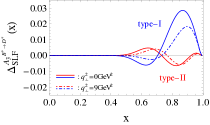
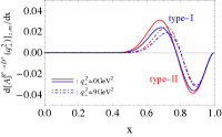
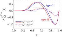
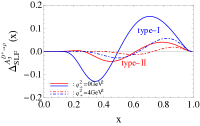
Based on these formulas, we have following discussions and findings:

• In Eq. (61), the first and the second term presents contribution to $A_{3}$ and $A_{4}$, respectively; the other terms correspond to the unphysical form factors. For convenience of discussion, we take the first term as an example and name it as $[{\cal\widetilde{B}}_{B}^{\mu}(\Gamma=\gamma^{\mu}\gamma_{5})]_{\rm term1}$. It can be easily found that $A_{3}$ could receive the contribution from $[{\cal\widetilde{B}}_{B}^{\mu}(\Gamma=\gamma^{\mu}\gamma_{5})]_{\rm term1}$ written as

  $${\widetilde{A}_{3}}^{\rm B}=4\frac{M^{\prime 2}-M^{\prime\prime 2}}{\epsilon^{\prime\prime*}\cdot q}\,\frac{\omega\cdot\epsilon^{\prime\prime*}}{\omega\cdot P}B_{1}^{(2)}\left(1+\frac{m_{1}^{\prime}-m_{1}^{\prime\prime}-2m_{2}}{D_{V,{\rm con}}^{\prime\prime}}\right)\,,$$ (64)

  which is dependent on the choice of $\lambda^{\prime\prime}$, i.e.,

  $${\widetilde{A}_{3}}^{\rm B}=\left\{\begin{array}[]{lr}4\frac{M^{\prime 2}-M^{\prime\prime 2}}{M^{\prime 2}-M^{\prime\prime 2}+q_{\bot}^{2}}B_{1}^{(2)}\left(1+\frac{m_{1}^{\prime}-m_{1}^{\prime\prime}-2m_{2}}{D_{V,{\rm con}}^{\prime\prime}}\right)\,,&\qquad\lambda^{\prime\prime}=0\\ 0\,.&\qquad\lambda^{\prime\prime}=\pm\\ \end{array}\right.$$ (65)

  Further considering the fact that ${\cal\widetilde{F}}^{\rm CLF}$ is independent of the choices of $\lambda^{\prime\,,\prime\prime}$, it can be found that $A_{3}$ in the CLF QM suffers from the problem of self-consistence, $[A_{3}]^{\rm full}_{\lambda^{\prime\prime}=0}\neq[A_{3}]^{\rm full}_{\lambda^{\prime\prime}=\pm}$, except that $A_{3}^{\rm B}$ vanishes at least numerically which is equivalent to the condition

  $$\int\frac{{\rm d}x{\rm d}^{2}{\bf k^{\prime}_{\bot}}}{2(2\pi)^{3}}\frac{\chi_{V}^{\prime}\chi_{V}^{\prime\prime}}{\bar{x}}B_{1}^{(2)}=0\,,\qquad\int\frac{{\rm d}x{\rm d}^{2}{\bf k^{\prime}_{\bot}}}{2(2\pi)^{3}}\frac{\chi_{V}^{\prime}\chi_{V}^{\prime\prime}}{\bar{x}}\frac{B_{1}^{(2)}}{D_{V}^{\prime\prime}}=0\,.$$ (66)

  In order to show clearly the performance of type-I and -II correspondence schemes, we take $B^{*}\to D^{*}$ transition as an example, and list the numerical results of $[A_{3}]^{\rm full}_{\lambda^{\prime\prime}=0}$, $[A_{3}]^{\rm full}_{\lambda^{\prime\prime}=\pm}$ and $[A_{3}]^{\rm CLF}$ at ${\bf q}_{\bot}^{2}=(0,2,4,9)\,{\rm GeV^{2}}$ in Table 3. In addition, we define the difference,

  $$\Delta^{\cal F}_{\rm full}(x)\equiv\frac{{\rm d}[{\cal F}]^{\rm full}_{\lambda^{\prime\prime}=0}}{{\rm d}x}-\frac{{\rm d}[{\cal F}]^{\rm full}_{\lambda^{\prime\prime}=\pm}}{{\rm d}x}\,,$$ (67)

  which is equal to $N_{c}\int\frac{{\rm d}^{2}{\bf k^{\prime}_{\bot}}}{2(2\pi)^{3}}\frac{\chi_{V}^{\prime}\chi_{V}^{\prime\prime}}{\bar{x}}{\widetilde{A}_{3}}^{\rm B}$ for $A_{3}$, and show $\Delta^{A_{3}}_{\rm full}(x)$ for $B^{*}\to D^{*}$ and $D^{*}\to\rho$ transitions in Fig. 2 (a) and (d). From these results, it can be easily found that such self-consistence condition is violated in the traditional type-I scheme, but can be satisfied by using the type-II scheme. Moreover, we have checked that all of the contributions of $B$ functions in Eqs. (61) and (62) vanish numerically within type-II scheme.

  Therefore, it can be concluded that the CLF results for the form factors of $V^{\prime}\to V^{\prime\prime}$ transition have the self-consistency problem within the type-I correspondence scheme, but it can be resolved by employing type-II scheme and moreover the unphysical form factors (for instance, the one corresponds to the third term in Eqs. (61)) vanish.

• In fact, the way to deal with the contributions of $B$ functions is ambiguous. For instance, instead of the treatment on $[{\cal\widetilde{B}}_{B}^{\mu}(\Gamma=\gamma^{\mu}\gamma_{5})]_{\rm term1}$ in the last item, we can also decompose $[{\cal\widetilde{B}}_{B}^{\mu}(\Gamma=\gamma^{\mu}\gamma_{5})]_{\rm term1}$ by using the identity

  $$P^{\mu}\frac{\epsilon\cdot\omega}{\omega\cdot P}= \epsilon^{\mu}-{\frac{q^{\mu}}{q^{2}}}\left({\epsilon\cdot q}-q\cdot P\frac{\omega\cdot\epsilon}{\omega\cdot P}\right)-\frac{\omega^{\mu}}{\omega\cdot P}\Big{[}\epsilon\cdot P-\epsilon\cdot q\frac{q\cdot P}{q^{2}}-\epsilon\cdot\omega\frac{P^{2}}{\omega\cdot P}$$

  $$+\epsilon\cdot\omega\frac{(q\cdot P)^{2}}{q^{2}\omega\cdot P}\Big{]}-\frac{i\lambda\,}{\,\omega\cdot P}\frac{\epsilon\cdot q}{q^{2}}\varepsilon^{\mu\alpha\beta\nu}\omega_{\alpha}q_{\beta}P_{\nu}\,,$$ (68)

  where, $\epsilon=\epsilon^{\prime\prime*}$. In Eq. (• ‣ 4), the second term vanishes in $[{\cal\widetilde{B}}_{B}^{\mu}(\Gamma=\gamma^{\mu}\gamma_{5})]_{\rm term1}$, and the last two terms would introduce more unphysical form factors. While, in this way, $A_{3}$ does not receive the contribution from $[{\cal\widetilde{B}}_{B}^{\mu}(\Gamma=\gamma^{\mu}\gamma_{5})]_{\rm term1}$ anymore; such contribution, as well as the corresponding self-consistence problem, transfers from $A_{3}$ to $A_{2}$ via the first term in Eq. (• ‣ 4).

  Therefore, it is hard to determine which form factor the $[{\cal\widetilde{B}}_{B}^{\mu}(\Gamma=\gamma^{\mu}\gamma_{5})]_{\rm term1}$ contributes to. This ambiguity results in significant uncertainty of CLF prediction, and thus is unacceptable. Fortunately, this problem exists only in the type-I scheme, and becomes trivial in the type-II scheme because all of the contributions related to $B$ functions vanish numerically.

• Besides of the self-consistency, the contributions of $B$ functions also result in the covariance problem because many terms in ${\cal\widetilde{B}}_{B}^{\mu}(\Gamma=\gamma^{\mu}\gamma_{5})$ and ${\cal\widetilde{B}}_{B}^{\mu}(\Gamma=\gamma^{\mu})$ are dependent on $\omega$, which violates the Lorentz covariance of ${\cal{B}}^{\mu}$. It can be clearly seen from Eqs. (61) and (62). The covariance problem caused by $B$ function contributions can not be avoided in the type-I scheme, but does not exist in the type-II scheme since, as has mentioned above, $B$ function contributions exist only in form and vanish numerically.

Besides of the CLF QM, the SLF QM also suffers from the problem of self-consistency. Again, we take $A_{3}$ as an example. In the section 2.2, $\lambda^{\prime}=\lambda^{\prime\prime}=\pm$ is taken in the calculation of $A_{3}$, and the result of $[{A}_{3}]^{\rm SLF}_{\lambda^{\prime}=\lambda^{\prime\prime}=\pm}$ given by Eq. (25) is obtained. Instead of such choice, one can also take $\lambda^{\prime}=0$ and $\lambda^{\prime\prime}=\pm$. In this way, we can obtain

$$\widetilde{A}_{3}^{{\rm SLF}}\big{|}_{\lambda^{\prime}=0,\lambda^{\prime\prime}=\pm} =\frac{-2(M^{\prime 2}-M^{\prime\prime 2})}{x\bar{x}M^{\prime}M^{\prime}_{0}q^{2}}\bigg{\{}\Big{[}{\bf k}_{\bot}^{\prime 2}+\bar{x}{\bf k^{\prime}_{\bot}\cdot q_{\bot}}-2\frac{({\bf k^{\prime}_{\bot}\cdot q_{\bot}})^{2}}{{\bf q}_{\bot}^{2}}\Big{]}\left({\bf k}_{\bot}^{\prime 2}+\bar{x}m_{1}^{\prime 2}+xm_{2}^{2}+x\bar{x}M_{0}^{\prime 2}\right)$$

$$+\frac{1}{D_{V,{\rm LF}}^{\prime\prime}}\Big{[}\Big{(}2\frac{({\bf k^{\prime}_{\bot}\cdot q_{\bot}})^{2}}{{\bf q}_{\bot}^{2}}-{\bf k}_{\bot}^{\prime 2}-\bar{x}{\bf k^{\prime}_{\bot}\cdot q_{\bot}}\Big{)}\Big{(}\left(m_{1}^{\prime}+m_{1}^{\prime\prime}\right)\left({\bf k}_{\bot}^{\prime 2}+xm_{2}^{2}+\bar{x}m_{1}^{\prime}m_{1}^{\prime\prime}+x\bar{x}M_{0}^{\prime 2}\right)$$

$$+\bar{x}m_{2}m_{1}^{\prime 2}-\bar{x}m_{2}m_{1}^{\prime\prime 2}+\bar{x}^{2}\left(m_{1}^{\prime}-m_{2}\right){\bf q}_{\bot}^{2}\Big{)}+x\bar{x}{\bf k_{\bot}^{\prime}\cdot k_{\bot}^{\prime\prime}}{\bf q}_{\bot}^{2}\left(m_{1}^{\prime}-m_{2}\right)$$

$$-{\bf k_{\bot}^{\prime\prime}\cdot q_{\bot}}\left[m_{1}^{\prime}{\bf k}_{\bot}^{\prime 2}+\left(\bar{x}m_{1}^{\prime}+xm_{2}\right)\left(m_{1}^{\prime}m_{2}+x\bar{x}M_{0}^{\prime 2}\right)\right]$$

$$-\bar{x}\left(m_{1}^{\prime}-m_{2}\right)\Big{(}4\frac{\left({\bf k^{\prime}_{\bot}\cdot q_{\bot}}\right)^{3}}{{\bf q}_{\bot}^{2}}-{\bf k^{\prime\prime}_{\bot}\cdot q_{\bot}}{\bf k}_{\bot}^{\prime 2}-2{\bf k^{\prime}_{\bot}\cdot q_{\bot}}{\bf k}_{\bot}^{\prime 2}-2\bar{x}\left({\bf k^{\prime}_{\bot}\cdot q_{\bot}}\right)^{2}\Big{)}\Big{]}$$

$$-\frac{1}{2x\bar{x}D_{V,{\rm LF}}^{\prime}D_{V,{\rm LF}}^{\prime\prime}}\left[\left(x-\bar{x}\right){\bf k}_{\bot}^{\prime 2}-\bar{x}m_{1}^{\prime 2}+xm_{2}^{2}-x\bar{x}\left(\bar{x}-x\right)M_{0}^{\prime 2}\right]\Big{[}{\bf k_{\bot}^{\prime\prime}\cdot q_{\bot}}\Big{(}x{\bf k}_{\bot}^{\prime 2}$$

$$-\bar{x}^{2}m_{1}^{\prime 2}+x^{2}m_{2}^{2}\Big{)}+4\bar{x}\frac{\left({\bf k^{\prime}_{\bot}\cdot q_{\bot}}\right)^{3}}{{\bf q}_{\bot}^{2}}-2\bar{x}^{2}\left({\bf k^{\prime}_{\bot}\cdot q_{\bot}}\right)^{2}-x\bar{x}{\bf k_{\bot}^{\prime}\cdot k_{\bot}^{\prime\prime}}{\bf q}_{\bot}^{2}-\bar{x}{\bf k^{\prime\prime}_{\bot}\cdot q_{\bot}}{\bf k}_{\bot}^{\prime 2}$$

$$-2\bar{x}{\bf k^{\prime}_{\bot}\cdot q_{\bot}}{\bf k}_{\bot}^{\prime 2}+\left(2\frac{({\bf k^{\prime}_{\bot}\cdot q_{\bot}})^{2}}{{\bf q}_{\bot}^{2}}-{\bf k}_{\bot}^{\prime 2}-\bar{x}{\bf k^{\prime}_{\bot}\cdot q_{\bot}}\right)\left(\bar{x}m_{1}^{\prime 2}-\bar{x}m_{1}^{\prime\prime 2}-\bar{x}^{2}{\bf q}_{\bot}^{2}\right)\Big{]}\bigg{\}}\,.$$ (69)

Comparing Eq. (25) with Eq. (69), it can be found that $[{A}_{3}]^{\rm SLF}_{\lambda^{\prime}=\lambda^{\prime\prime}=\pm}$ and $[{A}_{3}]^{\rm SLF}_{\lambda^{\prime}=0,\lambda^{\prime\prime}=\pm}$ are different from each other, which implies that the problem of self-consistency exists possibly also in the traditional SLF QM. In order to verify that, we take $B^{*}\to D^{*}$ transition as an example and list the numerical results of $[{A}_{3}]^{\rm SLF}_{\lambda^{\prime}=\lambda^{\prime\prime}=\pm}$ and $[{A}_{3}]^{\rm SLF}_{\lambda^{\prime}=0,\lambda^{\prime\prime}=\pm}$ in Table 3; meanwhile, we also show the difference, $\Delta^{A_{3}}_{\rm SLF}(x)$, defined as

$$\Delta^{A_{3}}_{\rm SLF}(x)\equiv\frac{{\rm d}[{A_{3}}]^{\rm SLF}_{\lambda^{\prime}=0,\lambda^{\prime\prime}=\pm}}{{\rm d}x}-\frac{{\rm d}[{A_{3}}]^{\rm SLF}_{\lambda^{\prime}=\lambda^{\prime\prime}=\pm}}{{\rm d}x}\,,$$ (70)

for $B^{*}\to D^{*}$ and $D^{*}\to\rho$ transitions in Fig. 2 (b)and (e). Form these results, it can be easily found that $[{A}_{3}]^{\rm SLF}_{\lambda^{\prime}=\lambda^{\prime\prime}=\pm}\neq[{A}_{3}]^{\rm SLF}_{\lambda^{\prime}=0,\lambda^{\prime\prime}=\pm}$ in the traditional SLF QM (named as type-I SLF QM for convince of discussion ); and meanwhile, it is interesting that the self-consistence can be recovered, because $[{A}_{3}]^{\rm SLF}_{\lambda^{\prime}=\lambda^{\prime\prime}=\pm}\dot{=}[{A}_{3}]^{\rm SLF}_{\lambda^{\prime}=0,\lambda^{\prime\prime}=\pm}$ numerically, when an additional replacement $M\to M_{0}$ (named as type-II SLF QM) is taken. Such replacement is also the main difference between type-I and -II correspondence schemes in the CLF QM.

Combining the findings mentioned above, we can conclude that the replacement $M\to M_{0}$ is necessary for the strict self-consistency and covariance of the CLF QM, as well as for the self-consistency of the SLF QM. This implies possibly that the effect of interaction has not yet been taken into account in a proper way at least in the SLF QM, which is easy to be understood since $\hat{M}^{2}=M_{0}^{2}+\hat{I}$ ($\hat{M}$ and $\hat{I}$ denote mass and interaction operators, respectively) in the LF dynamics. Therefore, the formulas for form factors with $M\to M_{0}$ should be treated as the results only at “leading-order” approximation or in the zero-binding-energy limit with “dressed” constituents [85, 55, 56, 57]. Further, mapping the CLF result to the corresponding SLF one, the type-II correspondence scheme is expected to be obtained, which will be checked in the following. In the mapping, in order to obtain the complete correspondence and avoid the effects of zero-mode contribution, one should use the valence contribution, $[{\cal F}]^{\rm val.}$, in the CLF QM instead of choosing only some special zero-mode independent quantities. Here, we take $A_{3}$ as an example again. Its valence result can be written as

$$\widetilde{A}_{3}^{\rm{val.}}= 4\Bigg{\{}\frac{{\bf k}_{\bot}^{\prime\prime}\cdot{\bf q}_{\bot}}{{\bf q}_{\bot}^{2}}\left(\frac{{\bf k}_{\bot}^{\prime 2}+m_{2}^{2}}{\bar{x}}-\bar{x}M^{\prime 2}\right)-{\bf k}_{\bot}^{\prime}\cdot{\bf k}_{\bot}^{\prime\prime}+\frac{1}{D_{V,{\rm con}}{{}^{\prime\prime}}}\bigg{[}{\bf k}_{\bot}^{\prime}\cdot{\bf k}_{\bot}^{\prime\prime}\left(m_{1}^{\prime}+m_{1}^{\prime\prime}\right)$$

$$-\frac{{\bf k}_{\bot}^{\prime\prime}\cdot{\bf q}_{\bot}}{{\bf q}_{\bot}^{2}}\left(\frac{{\bf k}_{\bot}^{\prime 2}+m_{2}^{2}}{\bar{x}}\left(m_{1}^{\prime}+m_{1}^{\prime\prime}\right)+\left(xm_{2}-\bar{x}m_{1}^{\prime\prime}\right)M^{\prime 2}-\left(\bar{x}m_{1}^{\prime}+xm_{2}\right)M^{\prime\prime 2}\right)\bigg{]}$$

$$-\frac{1}{D_{V,{\rm con}}^{\prime}D_{V,{\rm con}}^{\prime\prime}}\bigg{[}{\bf k}_{\bot}^{\prime}\cdot{\bf k}_{\bot}^{\prime\prime}\left(\frac{{\bf k}_{\bot}^{\prime 2}+m_{2}^{2}}{\bar{x}}-\bar{x}M^{\prime 2}\right)+\frac{{\bf k}_{\bot}^{\prime\prime}\cdot{\bf q}_{\bot}}{{\bf q}_{\bot}^{2}}{\bf k}_{\bot}^{\prime 2}\left(M^{\prime 2}-M^{\prime\prime 2}\right)$$

$$+2\bar{x}\left({\bf k}_{\bot}^{\prime}\cdot{\bf q}_{\bot}\right)^{2}-\bar{x}{\bf k}_{\bot}^{\prime 2}{\bf q}_{\bot}^{2}-{\bf k}_{\bot}^{\prime}\cdot{\bf q}_{\bot}{\bf k}_{\bot}^{\prime 2}\bigg{]}\Bigg{\}}\,.$$ (71)

Then, comparing $[{A}_{3}]^{\rm SLF}$ with $[{A}_{3}]^{\rm val.}$ (i.e., Eqs. (16,25) with Eqs. (49,71)), the type-II correspondence can be easily obtained. In other words, one can find that $[{A}_{3}]^{\rm SLF}=[{A}_{3}]^{\rm val.}$ in form within type-II correspondence scheme. This confirms again the finding,

$$[{\cal O}]^{\rm SLF}=[{\cal O}]^{\rm val.}\,,$$ (72)

obtained via $f_{V,A}$ and form factors of $P\to V$ transition in our previous works [86, 87].

The zero-mode contributions to a form factor can be obtained via $[{\cal F}]^{\rm CLF}=[{\cal F}]^{\rm val.}+[{\cal F}]^{\rm z.m.}$. In order to clearly show the effect of zero-mode contribution, we take $A_{3}^{B^{*}\to D^{*}\,,D^{*}\to\rho}$ as examples and plot the dependence of ${\rm d}[{\cal F}]^{\rm z.m.}/{\rm d}x$ on $x$ in Fig. 2 (c) and (f). It can be seen from these Figs that zero-mode presents nonzero contributions within the traditional type-I correspondence scheme; while, in the type-II correspondence scheme, these contributions, although existing formally, vanish numerically, i.e., $[A_{3}(q^{2})]_{\rm z.m.}\dot{=}0$ (type-II), because the contribution with small $x$ and the one with large $x$ cancel each other out exactly at each ${{\bf q}_{\bot}^{2}}$ point. From such finding, one can further conclude that

$$[{\cal O}]^{\rm val.}\,\dot{=}\,[{\cal O}]^{\rm CLF}\,,$$ (73)

which can also be found from the numerical example given in Table 3. This confirms Eq. (1) mentioned in the introduction.

Figure 3: $q^{2}$ (in unit of $\rm GeV^{2}$) dependence of form factors of $c\to(s,q)$ induced $D^{*}\to(K^{*}\,,\rho)$, $D^{*}_{s}\to(\phi\,,K^{*})$, $J/\Psi\to(D^{*}_{s}\,,D^{*})$, $B^{*}_{c}\to(B^{*}_{s}\,,B^{*})$ transitions with the parameterization scheme given by Eq. (75). The dots in the space-like region are the results obtained directly via LFQMs, and the lines are fitting results.

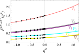
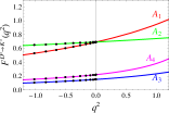
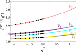
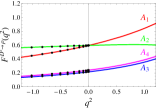
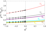
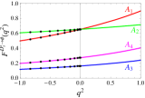
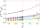
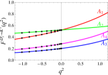
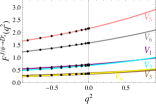
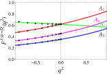
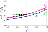
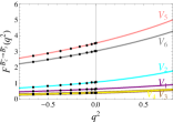
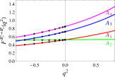
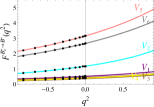
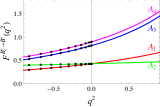
Figure 4: $q^{2}$ (in unit of $\rm GeV^{2}$) dependence of form factors of $b\to(c,s,q)$ induced $B^{*}\to(D^{*}\,,K^{*}\,,\rho)$, $B^{*}_{s}\to(D^{*}_{s}\,,\phi\,,K^{*})$, $B^{*}_{c}\to(J/\Psi\,,D^{*}_{s}\,,D^{*})$, $\Upsilon(1S)\to(B_{c}^{*}\,,B_{s}^{*}\,,B^{*})$ transitions with the parameterization scheme given by Eq. (75). The other captions are the same as in Fig. 3.

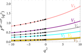
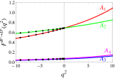
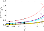
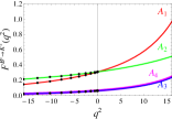
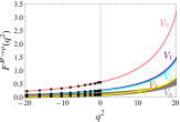
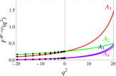
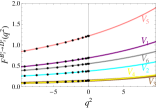
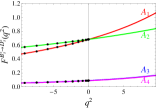
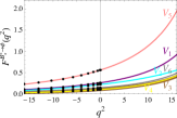
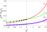
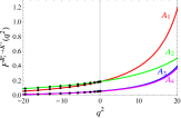
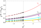
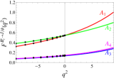
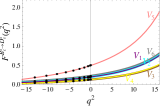
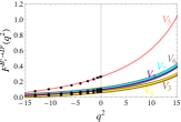
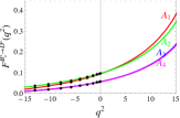
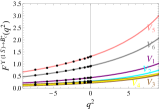
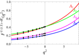
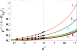
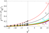
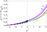
Table 4: Fitting results for the form factors of $c\to(q,s)$ induced $D^{*}\to(\rho\,,K^{*})$, $D^{*}_{s}\to(K^{*}\,,\phi)$, $J/\Psi\to(D^{*}\,,D^{*}_{s})$, $B^{*}_{c}\to(B^{*}\,,B^{*}_{s})$ transitions with the parameterization scheme given by Eq. (75). The errors are due to parameters $\beta$ and quark masses only (cf. section 4 for a more complete discussion).

	${\cal F}(0)$	$a$	$b_{1}$		${\cal F}(0)$	$a$	$b_{1}$
$V_{1}^{D^{*}\to\rho}$	$0.65_{-0.01-0.09}^{+0.01+0.09}$	$0.96_{-0.02-0.23}^{+0.01+0.28}$	$-2.40_{-0.03-0.03}^{+0.03+0.02}$	$V_{1}^{D^{*}\to K^{*}}$	$0.74_{-0.02-0.10}^{+0.01+0.09}$	$0.87_{-0.01-0.23}^{+0.01+0.35}$	$-2.48_{-0.01-0.54}^{+0.01+0.42}$
$V_{2}^{D^{*}\to\rho}$	$0.51_{-0.02-0.04}^{+0.02+0.03}$	$1.07_{-0.01-0.30}^{+0.01+0.37}$	$-2.31_{-0.04-0.06}^{+0.04+0.11}$	$V_{2}^{D^{*}\to K^{*}}$	$0.43_{-0.03-0.08}^{+0.03+0.03}$	$0.93_{-0.03-0.20}^{+0.02+0.21}$	$-2.33_{-0.07-0.32}^{+0.05+0.33}$
$V_{3}^{D^{*}\to\rho}$	$0.29_{-0.00-0.03}^{+0.00+0.03}$	$1.11_{-0.00-0.20}^{+0.01+0.31}$	$-3.35_{-0.02-0.17}^{+0.02+0.30}$	$V_{3}^{D^{*}\to K^{*}}$	$0.26_{-0.01-0.02}^{+0.01+0.02}$	$0.98_{-0.01-0.26}^{+0.02+0.20}$	$-3.46_{-0.14-0.45}^{+0.12+0.41}$
$V_{4}^{D^{*}\to\rho}$	$0.29_{-0.00-0.03}^{+0.00+0.03}$	$1.32_{-0.01-0.20}^{+0.01+0.31}$	$-4.94_{-0.17-0.56}^{+0.17+0.61}$	$V_{4}^{D^{*}\to K^{*}}$	$0.26_{-0.01-0.02}^{+0.01+0.02}$	$1.11_{-0.02-0.39}^{+0.02+0.47}$	$-4.14_{-0.10-0.74}^{+0.09+0.62}$
$V_{5}^{D^{*}\to\rho}$	$1.42_{-0.02-0.17}^{+0.02+0.17}$	$0.94_{-0.00-0.22}^{+0.01+0.26}$	$-2.08_{-0.04-0.12}^{+0.06+0.18}$	$V_{5}^{D^{*}\to K^{*}}$	$1.50_{-0.03-0.16}^{+0.02+0.12}$	$0.85_{-0.00-0.03}^{+0.01+0.05}$	$-2.19_{-0.03-0.12}^{+0.03+0.15}$
$V_{6}^{D^{*}\to\rho}$	$0.68_{-0.01-0.17}^{+0.01+0.17}$	$0.86_{-0.00-0.22}^{+0.01+0.31}$	$-2.10_{-0.04-0.31}^{+0.05+0.26}$	$V_{6}^{D^{*}\to K^{*}}$	$0.78_{-0.02-0.17}^{+0.02+0.23}$	$0.82_{-0.02-0.18}^{+0.02+0.25}$	$-2.19_{-0.02-0.35}^{+0.02+0.29}$
$A_{1}^{D^{*}\to\rho}$	$0.59_{-0.01-0.07}^{+0.01+0.07}$	$0.95_{-0.01-0.22}^{+0.01+0.23}$	$-2.30_{-0.03-0.06}^{+0.03+0.06}$	$A_{1}^{D^{*}\to K^{*}}$	$0.69_{-0.01-0.09}^{+0.01+0.08}$	$0.87_{-0.01-0.11}^{+0.01+0.10}$	$-2.40_{-0.02-0.07}^{+0.02+0.07}$
$A_{2}^{D^{*}\to\rho}$	$0.59_{-0.01-0.07}^{+0.01+0.07}$	$1.72_{-0.05-0.07}^{+0.05+0.08}$	$12.08_{-0.21-0.49}^{+0.25+0.52}$	$A_{2}^{D^{*}\to K^{*}}$	$0.69_{-0.01-0.09}^{+0.01+0.08}$	$1.04_{-0.03-0.06}^{+0.05+0.07}$	$6.47_{-0.05-0.50}^{+0.03+0.53}$
$A_{3}^{D^{*}\to\rho}$	$0.22_{-0.01-0.03}^{+0.01+0.03}$	$1.27_{-0.01-0.35}^{+0.01+0.43}$	$-3.84_{-0.12-0.39}^{+0.11+0.50}$	$A_{3}^{D^{*}\to K^{*}}$	$0.15_{-0.01-0.04}^{+0.01+0.02}$	$1.09_{-0.04-0.19}^{+0.03+0.22}$	$-3.78_{-0.13-0.24}^{+0.11+0.25}$
$A_{4}^{D^{*}\to\rho}$	$0.24_{-0.01-0.04}^{+0.01+0.06}$	$1.23_{-0.01-0.34}^{+0.02+0.41}$	$-3.78_{-0.05-0.32}^{+0.03+0.23}$	$A_{4}^{D^{*}\to K^{*}}$	$0.22_{-0.01-0.03}^{+0.01+0.05}$	$1.07_{-0.02-0.15}^{+0.02+0.21}$	$-3.93_{-0.12-0.42}^{+0.12+0.51}$
$V_{1}^{D_{s}^{*}\to K^{*}}$	$0.58_{-0.02-0.09}^{+0.02+0.10}$	$0.98_{-0.01-0.21}^{+0.01+0.29}$	$-3.35_{-0.04-0.09}^{+0.03+0.15}$	$V_{1}^{D_{s}^{*}\to\phi}$	$0.71_{-0.01-0.10}^{+0.01+0.09}$	$0.94_{-0.01-0.11}^{+0.01+0.11}$	$-3.25_{-0.07-0.09}^{+0.07+0.14}$
$V_{2}^{D_{s}^{*}\to K^{*}}$	$0.42_{-0.04-0.03}^{+0.04+0.02}$	$1.06_{-0.03-0.27}^{+0.02+0.33}$	$-3.12_{-0.11-0.22}^{+0.09+0.30}$	$V_{2}^{D_{s}^{*}\to\phi}$	$0.38_{-0.03-0.11}^{+0.03+0.04}$	$0.98_{-0.05-0.06}^{+0.04+0.04}$	$-3.00_{-0.14-0.25}^{+0.12+0.28}$
$V_{3}^{D_{s}^{*}\to K^{*}}$	$0.30_{-0.01-0.03}^{+0.00+0.03}$	$1.06_{-0.02-0.27}^{+0.02+0.34}$	$-3.77_{-0.10-0.25}^{+0.12+0.33}$	$V_{3}^{D_{s}^{*}\to\phi}$	$0.28_{-0.01-0.02}^{+0.01+0.02}$	$1.00_{-0.04-0.25}^{+0.04+0.30}$	$-3.76_{-0.14-0.34}^{+0.14+0.43}$
$V_{4}^{D_{s}^{*}\to K^{*}}$	$0.30_{-0.01-0.03}^{+0.00+0.03}$	$1.24_{-0.04-0.34}^{+0.03+0.30}$	$-4.26_{-0.51-0.37}^{+0.45+0.49}$	$V_{4}^{D_{s}^{*}\to\phi}$	$0.28_{-0.01-0.02}^{+0.01+0.02}$	$1.13_{-0.06-0.30}^{+0.04+0.39}$	$-3.98_{-0.48-0.36}^{+0.35+0.47}$
$V_{5}^{D_{s}^{*}\to K^{*}}$	$1.36_{-0.04-0.20}^{+0.04+0.19}$	$0.95_{-0.01-0.20}^{+0.01+0.27}$	$-2.87_{-0.05-0.22}^{+0.05+0.28}$	$V_{5}^{D_{s}^{*}\to\phi}$	$1.54_{-0.03-0.16}^{+0.02+0.16}$	$0.91_{-0.01-0.18}^{+0.01+0.23}$	$-2.82_{-0.08-0.49}^{+0.09+0.43}$
$V_{6}^{D_{s}^{*}\to K^{*}}$	$0.68_{-0.03-0.15}^{+0.03+0.21}$	$0.91_{-0.02-0.23}^{+0.02+0.30}$	$-2.89_{-0.05-0.46}^{+0.03+0.45}$	$V_{6}^{D_{s}^{*}\to\phi}$	$0.86_{-0.02-0.19}^{+0.02+0.25}$	$0.91_{-0.03-0.23}^{+0.03+0.25}$	$-2.70_{-0.18-0.35}^{+0.18+0.33}$
$A_{1}^{D_{s}^{*}\to K^{*}}$	$0.52_{-0.02-0.08}^{+0.02+0.07}$	$0.98_{-0.01-0.21}^{+0.01+0.28}$	$-3.25_{-0.04-0.12}^{+0.04+0.20}$	$A_{1}^{D_{s}^{*}\to\phi}$	$0.65_{-0.01-0.09}^{+0.01+0.08}$	$0.94_{-0.01-0.16}^{+0.01+0.17}$	$-3.17_{-0.07-0.11}^{+0.07+0.17}$
$A_{2}^{D_{s}^{*}\to K^{*}}$	$0.52_{-0.02-0.08}^{+0.02+0.08}$	$0.05_{-0.01-0.04}^{+0.01+0.03}$	$-3.07_{-0.11-0.70}^{+0.19+0.87}$	$A_{2}^{D_{s}^{*}\to\phi}$	$0.65_{-0.01-0.09}^{+0.01+0.08}$	$1.06_{-0.05-0.16}^{+0.04+0.14}$	$6.17_{-0.12-0.17}^{+0.09+0.15}$
$A_{3}^{D_{s}^{*}\to K^{*}}$	$0.20_{-0.02-0.03}^{+0.02+0.03}$	$1.21_{-0.04-0.34}^{+0.03+0.36}$	$-4.22_{-0.17-0.44}^{+0.15+0.40}$	$A_{3}^{D_{s}^{*}\to\phi}$	$0.16_{-0.01-0.05}^{+0.01+0.02}$	$1.10_{-0.07-0.07}^{+0.05+0.07}$	$-4.04_{-0.21-0.16}^{+0.14+0.20}$
$A_{4}^{D_{s}^{*}\to K^{*}}$	$0.28_{-0.01-0.05}^{+0.01+0.04}$	$1.16_{-0.03-0.24}^{+0.03+0.30}$	$-4.28_{-0.24-0.25}^{+0.23+0.27}$	$A_{4}^{D_{s}^{*}\to\phi}$	$0.27_{-0.01-0.04}^{+0.01+0.05}$	$1.12_{-0.06-0.31}^{+0.05+0.39}$	$-4.10_{-0.10-0.58}^{+0.07+0.40}$
$V_{1}^{J/\psi\to D^{*}}$	$0.55_{-0.02-0.12}^{+0.02+0.12}$	$1.09_{-0.02-0.15}^{+0.02+0.13}$	$-13.71_{-0.25-0.66}^{+0.26+0.53}$	$V_{1}^{J/\psi\to D_{s}^{*}}$	$0.72_{-0.02-0.13}^{+0.01+0.12}$	$0.97_{-0.03-0.14}^{+0.03+0.18}$	$-11.44_{-0.58-1.30}^{+0.54+1.26}$
$V_{2}^{J/\psi\to D^{*}}$	$0.60_{-0.05-0.10}^{+0.05+0.15}$	$1.37_{-0.03-0.41}^{+0.02+0.47}$	$-14.80_{-0.08-3.17}^{+0.05+2.59}$	$V_{2}^{J/\psi\to D_{s}^{*}}$	$0.68_{-0.06-0.11}^{+0.06+0.14}$	$1.23_{-0.03-0.36}^{+0.03+0.35}$	$-12.59_{-0.53-3.17}^{+0.51+2.97}$
$V_{3}^{J/\psi\to D^{*}}$	$0.36_{-0.01-0.03}^{+0.01+0.03}$	$1.20_{-0.02-0.32}^{+0.02+0.34}$	$-12.66_{-0.48-2.33}^{+0.52+2.22}$	$V_{3}^{J/\psi\to D_{s}^{*}}$	$0.36_{-0.01-0.02}^{+0.01+0.01}$	$1.17_{-0.02-0.32}^{+0.02+0.40}$	$-11.59_{-0.35-1.48}^{+0.35+2.15}$
$V_{4}^{J/\psi\to D^{*}}$	$0.36_{-0.01-0.03}^{+0.01+0.03}$	$1.37_{-0.02-0.36}^{+0.02+0.42}$	$-14.02_{-0.34-2.40}^{+0.31+2.31}$	$V_{4}^{J/\psi\to D_{s}^{*}}$	$0.36_{-0.01-0.02}^{+0.01+0.01}$	$1.33_{-0.02-0.36}^{+0.02+0.36}$	$-14.33_{-0.04-1.82}^{+0.06+2.57}$
$V_{5}^{J/\psi\to D^{*}}$	$1.79_{-0.05-0.34}^{+0.05+0.52}$	$1.06_{-0.02-0.27}^{+0.02+0.27}$	$-12.48_{-0.22-1.94}^{+0.21+1.75}$	$V_{5}^{J/\psi\to D_{s}^{*}}$	$2.16_{-0.04-0.36}^{+0.04+0.51}$	$0.96_{-0.02-0.22}^{+0.03+0.30}$	$-10.41_{-0.27-2.19}^{+0.26+2.28}$
$V_{6}^{J/\psi\to D^{*}}$	$1.23_{-0.05-0.34}^{+0.04+0.53}$	$1.33_{-0.05-0.30}^{+0.06+0.32}$	$-7.22_{-0.30-1.72}^{+0.35+1.43}$	$V_{6}^{J/\psi\to D_{s}^{*}}$	$1.58_{-0.04-0.40}^{+0.04+0.58}$	$0.89_{-0.04-0.22}^{+0.03+0.31}$	$-10.50_{-0.32-2.37}^{+0.30+2.40}$
$A_{1}^{J/\psi\to D^{*}}$	$0.47_{-0.01-0.09}^{+0.01+0.09}$	$1.10_{-0.03-0.06}^{+0.03+0.08}$	$-13.60_{-0.26-0.70}^{+0.26+0.52}$	$A_{1}^{J/\psi\to D_{s}^{*}}$	$0.62_{-0.01-0.10}^{+0.01+0.08}$	$0.98_{-0.03-0.15}^{+0.03+0.17}$	$-11.35_{-0.25-0.73}^{+0.31+1.12}$
$A_{2}^{J/\psi\to D^{*}}$	$0.47_{-0.01-0.09}^{+0.01+0.09}$	$0.72_{-0.02-0.17}^{+0.02+0.18}$	$7.17_{-0.19-1.18}^{+0.23+1.30}$	$A_{2}^{J/\psi\to D_{s}^{*}}$	$0.62_{-0.01-0.10}^{+0.01+0.08}$	$0.50_{-0.09-0.21}^{+0.09+0.27}$	$20.69_{-1.27-4.02}^{+1.19+5.33}$
$A_{3}^{J/\psi\to D^{*}}$	$0.38_{-0.01-0.08}^{+0.01+0.11}$	$1.41_{-0.01-0.30}^{+0.01+0.34}$	$-14.69_{-0.08-2.21}^{+0.05+2.84}$	$A_{3}^{J/\psi\to D_{s}^{*}}$	$0.35_{-0.01-0.06}^{+0.01+0.07}$	$1.35_{-0.01-0.27}^{+0.01+0.35}$	$-13.69_{-0.30-2.84}^{+0.21+3.12}$
$A_{4}^{J/\psi\to D^{*}}$	$0.45_{-0.01-0.11}^{+0.01+0.15}$	$1.32_{-0.03-0.27}^{+0.02+0.26}$	$-14.00_{-0.33-2.58}^{+0.28+2.55}$	$A_{4}^{J/\psi\to D_{s}^{*}}$	$0.45_{-0.01-0.09}^{+0.01+0.13}$	$1.26_{-0.03-0.35}^{+0.02+0.45}$	$-12.91_{-0.36-2.79}^{+0.20+2.49}$
$V_{1}^{B_{c}^{*}\to B^{*}}$	$0.52_{-0.02-0.11}^{+0.02+0.11}$	$1.18_{-0.03-0.16}^{+0.03+0.24}$	$-92.66_{-0.25-1.25}^{+0.23+2.13}$	$V_{1}^{B_{c}^{*}\to B_{s}^{*}}$	$0.63_{-0.01-0.12}^{+0.01+0.12}$	$1.17_{-0.02-0.17}^{+0.01+0.23}$	$-86.23_{-0.61-1.48}^{+0.58+1.31}$
$V_{2}^{B_{c}^{*}\to B^{*}}$	$1.18_{-0.13-0.28}^{+0.13+0.30}$	$1.63_{-0.03-0.38}^{+0.03+0.46}$	$-109.58_{-0.10-14.01}^{+0.14+14.65}$	$V_{2}^{B_{c}^{*}\to B_{s}^{*}}$	$1.06_{-0.11-0.40}^{+0.11+0.20}$	$1.74_{-0.03-0.44}^{+0.03+0.55}$	$-96.20_{-1.02-1.52}^{+0.98+1.92}$
$V_{3}^{B_{c}^{*}\to B^{*}}$	$0.40_{-0.01-0.04}^{+0.01+0.03}$	$1.30_{-0.04-0.26}^{+0.04+0.34}$	$-81.00_{-0.49-2.30}^{+0.53+2.47}$	$V_{3}^{B_{c}^{*}\to B_{s}^{*}}$	$0.40_{-0.01-0.03}^{+0.01+0.01}$	$1.33_{-0.03-0.27}^{+0.03+0.33}$	$-77.08_{-0.73-3.07}^{+0.68+3.56}$
$V_{4}^{B_{c}^{*}\to B^{*}}$	$0.40_{-0.01-0.04}^{+0.01+0.03}$	$1.40_{-0.04-0.37}^{+0.03+0.41}$	$-84.44_{-0.58-3.01}^{-0.61+3.25}$	$V_{4}^{B_{c}^{*}\to B_{s}^{*}}$	$0.40_{-0.01-0.03}^{+0.01+0.01}$	$1.42_{-0.02-0.26}^{+0.02+0.34}$	$-80.47_{-1.57-5.81}^{+1.49+6.00}$
$V_{5}^{B_{c}^{*}\to B^{*}}$	$3.15_{-0.11-0.82}^{+0.10+1.12}$	$1.16_{-0.02-0.21}^{+0.02+0.29}$	$-88.43_{-0.04-5.82}^{+0.04+8.03}$	$V_{5}^{B_{c}^{*}\to B_{s}^{*}}$	$3.52_{-0.06-0.87}^{+0.06+1.12}$	$1.16_{-0.02+0.21}^{+0.01+0.28}$	$-82.15_{-0.85-5.10}^{+0.85+8.23}$
$V_{6}^{B_{c}^{*}\to B^{*}}$	$2.66_{-0.10-0.79}^{+0.10+1.11}$	$1.14_{-0.03-0.21}^{+0.03+0.29}$	$-89.98_{-0.31-6.80}^{+0.24+7.69}$	$V_{6}^{B_{c}^{*}\to B_{s}^{*}}$	$3.02_{-0.06-0.85}^{+0.06+1.15}$	$1.13_{-0.02-0.21}^{+0.01+0.29}$	$-83.43_{-0.66-6.58}^{+0.64+8.16}$
$A_{1}^{B_{c}^{*}\to B^{*}}$	$0.43_{-0.02-0.08}^{+0.01+0.07}$	$1.18_{-0.03-0.17}^{+0.02+0.16}$	$-92.23_{-0.29-2.02}^{+0.25+1.99}$	$A_{1}^{B_{c}^{*}\to B_{s}^{*}}$	$0.53_{-0.01-0.09}^{+0.01+0.08}$	$1.17_{-0.01-0.17}^{+0.01+0.25}$	$-85.77_{-0.70-1.03}^{+0.66+1.36}$
$A_{2}^{B_{c}^{*}\to B^{*}}$	$0.43_{-0.02-0.08}^{+0.01+0.07}$	$0.66_{-0.01-0.24}^{+0.01+0.25}$	$37.14_{-0.07-7.22}^{+0.06+7.01}$	$A_{2}^{B_{c}^{*}\to B_{s}^{*}}$	$0.53_{-0.01-0.09}^{+0.01+0.08}$	$0.67_{-0.08-0.17}^{+0.09+0.25}$	$71.55_{-1.80-7.33}^{+2.42+8.44}$
$A_{3}^{B_{c}^{*}\to B^{*}}$	$0.81_{-0.03-0.20}^{+0.03+0.25}$	$1.56_{-0.01-0.35}^{+0.01+0.40}$	$-94.78_{-0.60-5.14}^{+0.73+7.38}$	$A_{3}^{B_{c}^{*}\to B_{s}^{*}}$	$0.73_{-0.02-0.15}^{+0.02+0.16}$	$1.59_{-0.01-0.37}^{+0.01+0.41}$	$-88.56_{-1.59-5.53}^{+1.90+6.86}$
$A_{4}^{B_{c}^{*}\to B^{*}}$	$0.89_{-0.02-0.24}^{+0.02+0.32}$	$1.49_{-0.04-0.33}^{+0.04+0.45}$	$-93.00_{-0.94-5.58}^{+0.91+7.77}$	$A_{4}^{B_{c}^{*}\to B_{s}^{*}}$	$0.85_{-0.01-0.20}^{+0.01+0.25}$	$1.60_{-0.12-0.33}^{+0.10+0.32}$	$-80.22_{-1.29-8.29}^{+1.57+9.02}$

Table 5: Same as Table 4 except for $b\to(q,s,c)$ induced $B^{*}\to(\rho\,,K^{*}\,,D^{*})$ and $B_{s}\to(K^{*}\,,\phi\,,D^{*}_{s})$ transitions. The errors are due to parameters $\beta$ and quark masses only (cf. section 4 for a more complete discussion).

	${\cal F}(0)$	$a$	$b_{1}$		${\cal F}(0)$	$a$	$b_{1}$
$V_{1}^{B^{*}\to\rho}$	$0.27_{-0.01-0.04}^{+0.01+0.05}$	$0.99_{-0.01-0.05}^{+0.01+0.04}$	$-3.25_{-0.15-0.24}^{+0.14+0.12}$	$V_{1}^{B^{*}\to K^{*}}$	$0.31_{-0.01-0.06}^{+0.01+0.06}$	$1.00_{-0.01-0.08}^{+0.01+0.07}$	$-3.28_{-0.06-0.12}^{+0.05+0.10}$
$V_{2}^{B^{*}\to\rho}$	$0.25_{-0.01-0.03}^{+0.01+0.03}$	$1.00_{-0.04-0.05}^{+0.03+0.05}$	$-3.34_{-0.06-0.14}^{+0.06+0.22}$	$V_{2}^{B^{*}\to K^{*}}$	$0.26_{-0.01-0.04}^{+0.01+0.03}$	$1.00_{-0.05-0.06}^{+0.03+0.05}$	$-3.27_{-0.16-0.17}^{+0.12+0.09}$
$V_{3}^{B^{*}\to\rho}$	$0.10_{-0.00-0.01}^{-0.00+0.02}$	$1.00_{-0.01-0.03}^{+0.00+0.02}$	$-5.91_{-0.13-0.50}^{+0.09+0.38}$	$V_{3}^{B^{*}\to K^{*}}$	$0.11_{-0.00-0.02}^{-0.00+0.02}$	$0.98_{-0.00-0.02}^{+0.01+0.01}$	$-5.18_{-0.08-0.41}^{+0.16+0.34}$
$V_{4}^{B^{*}\to\rho}$	$0.10_{-0.00-0.01}^{+0.00+0.02}$	$0.99_{-0.00-0.01}^{+0.01+0.01}$	$-5.91_{-0.09-0.43}^{+0.14+0.36}$	$V_{4}^{B^{*}\to K^{*}}$	$0.11_{-0.00-0.02}^{+0.00+0.02}$	$0.99_{-0.00-0.04}^{+0.00+0.04}$	$-5.69_{-0.09-0.32}^{+0.09+0.27}$
$V_{5}^{B^{*}\to\rho}$	$0.57_{-0.01-0.09}^{+0.01+0.10}$	$1.00_{-0.01-0.08}^{+0.01+0.06}$	$-3.10_{-0.07-0.18}^{+0.05+0.13}$	$V_{5}^{B^{*}\to K^{*}}$	$0.65_{-0.02-0.11}^{+0.02+0.11}$	$0.99_{-0.01-0.05}^{+0.01+0.04}$	$-3.17_{-0.13-0.14}^{+0.13+0.09}$
$V_{6}^{B^{*}\to\rho}$	$0.12_{-0.00-0.02}^{+0.00+0.03}$	$0.89_{-0.01-0.01}^{+0.00+0.02}$	$-3.24_{-0.11-0.35}^{+0.11+0.31}$	$V_{6}^{B^{*}\to K^{*}}$	$0.15_{-0.01-0.03}^{+0.01+0.04}$	$0.90_{-0.01-0.04}^{+0.00+0.09}$	$-3.34_{-0.15-0.20}^{+0.15+0.19}$
$A_{1}^{B^{*}\to\rho}$	$0.26_{-0.01-0.04}^{+0.01+0.05}$	$0.99_{-0.02-0.04}^{+0.01+0.04}$	$-3.21_{-0.17-0.23}^{+0.14+0.11}$	$A_{1}^{B^{*}\to K^{*}}$	$0.31_{-0.01-0.06}^{+0.01+0.06}$	$0.98_{-0.01-0.05}^{+0.01+0.04}$	$-3.28_{-0.03-0.22}^{+0.01+0.19}$
$A_{2}^{B^{*}\to\rho}$	$0.26_{-0.01-0.04}^{+0.01+0.05}$	$0.51_{-0.01-0.06}^{+0.01+0.07}$	$-1.14_{-0.01-0.13}^{+0.02+0.15}$	$A_{2}^{B^{*}\to K^{*}}$	$0.31_{-0.01-0.06}^{+0.01+0.06}$	$0.55_{-0.06-0.15}^{+0.03+0.14}$	$-1.21_{-0.20-0.28}^{+0.11+0.24}$
$A_{3}^{B^{*}\to\rho}$	$0.07_{-0.00-0.01}^{+0.00+0.01}$	$1.00_{-0.00-0.01}^{+0.01+0.01}$	$-5.39_{-0.03-0.59}^{+0.07+0.56}$	$A_{3}^{B^{*}\to K^{*}}$	$0.06_{-0.00-0.01}^{+0.00+0.01}$	$1.00_{-0.02-0.01}^{+0.00+0.01}$	$-5.48_{-0.03-0.64}^{+0.01+0.51}$
$A_{4}^{B^{*}\to\rho}$	$0.06_{-0.00-0.01}^{+0.00+0.01}$	$0.99_{-0.00-0.01}^{+0.01+0.02}$	$-5.38_{-0.12-0.61}^{+0.21+0.48}$	$A_{4}^{B^{*}\to K^{*}}$	$0.07_{-0.00-0.01}^{+0.00+0.01}$	$0.98_{-0.01-0.02}^{+0.01+0.01}$	$-5.56_{-0.09-0.55}^{+0.05+0.41}$
$V_{1}^{B^{*}\to D^{*}}$	$0.70_{-0.01-0.11}^{+0.01+0.10}$	$1.13_{-0.01-0.07}^{+0.01+0.07}$	$-2.54_{-0.01-0.20}^{+0.01+0.15}$	$V_{1}^{B_{s}^{*}\to K^{*}}$	$0.19_{-0.01-0.05}^{+0.01+0.06}$	$1.00_{-0.02-0.02}^{+0.01+0.02}$	$-5.12_{-0.24-0.20}^{+0.24+0.17}$
$V_{2}^{B^{*}\to D^{*}}$	$0.35_{-0.01-0.04}^{+0.01+0.02}$	$1.15_{-0.01-0.07}^{+0.01+0.05}$	$-2.51_{-0.02-0.16}^{+0.03+0.23}$	$V_{2}^{B_{s}^{*}\to K^{*}}$	$0.18_{-0.01-0.04}^{+0.01+0.04}$	$1.00_{-0.01-0.02}^{+0.01+0.02}$	$-5.14_{-0.23-0.18}^{+0.21+0.17}$
$V_{3}^{B^{*}\to D^{*}}$	$0.12_{-0.00-0.01}^{+0.00+0.02}$	$1.39_{-0.02-0.25}^{+0.01+0.13}$	$-4.05_{-0.06-1.02}^{+0.06+0.47}$	$V_{3}^{B_{s}^{*}\to K^{*}}$	$0.09_{-0.01-0.02}^{+0.01+0.02}$	$0.98_{-0.01-0.02}^{+0.02+0.02}$	$-6.37_{-0.20-0.33}^{+0.23+0.26}$
$V_{4}^{B^{*}\to D^{*}}$	$0.12_{-0.00-0.01}^{+0.00+0.02}$	$1.47_{-0.01-0.40}^{+0.01+0.39}$	$-4.27_{-0.03-0.99}^{+0.03+0.78}$	$V_{4}^{B_{s}^{*}\to K^{*}}$	$0.09_{-0.01-0.02}^{+0.01+0.02}$	$1.00_{-0.02-0.03}^{+0.01+0.02}$	$-7.00_{-0.18-0.30}^{+0.17+0.17}$
$V_{5}^{B^{*}\to D^{*}}$	$1.19_{-0.01-0.14}^{+0.01+0.09}$	$1.13_{-0.02-0.08}^{+0.01+0.06}$	$-2.48_{-0.06-0.21}^{+0.05+0.13}$	$V_{5}^{B_{s}^{*}\to K^{*}}$	$0.42_{-0.03-0.10}^{+0.02+0.12}$	$1.00_{-0.03-0.03}^{+0.02+0.04}$	$-4.95_{-0.30-0.19}^{+0.27+0.21}$
$V_{6}^{B^{*}\to D^{*}}$	$0.51_{-0.01-0.13}^{+0.01+0.15}$	$1.13_{-0.02-0.09}^{+0.01+0.07}$	$-2.43_{-0.05-0.21}^{+0.02+0.18}$	$V_{6}^{B_{s}^{*}\to K^{*}}$	$0.10_{-0.01-0.03}^{+0.01+0.03}$	$1.00_{-0.01-0.02}^{+0.02+0.01}$	$-4.62_{-0.17-0.17}^{+0.19+0.15}$
$A_{1}^{B^{*}\to D^{*}}$	$0.69_{-0.01-0.11}^{+0.01+0.10}$	$1.13_{-0.01-0.07}^{+0.01+0.07}$	$-2.52_{-0.01-0.21}^{+0.01+0.24}$	$A_{1}^{B_{s}^{*}\to K^{*}}$	$0.19_{-0.01-0.05}^{+0.01+0.05}$	$0.99_{-0.02-0.04}^{+0.02+0.03}$	$-5.09_{-0.13-0.06}^{+0.07+0.05}$
$A_{2}^{B^{*}\to D^{*}}$	$0.69_{-0.01-0.11}^{+0.01+0.10}$	$0.80_{-0.04-0.15}^{+0.04+0.14}$	$0.24_{-0.14-0.13}^{+0.08+0.17}$	$A_{2}^{B_{s}^{*}\to K^{*}}$	$0.19_{-0.01-0.05}^{+0.01+0.05}$	$0.61_{-0.03-0.02}^{+0.03+0.03}$	$-3.12_{-0.17-0.32}^{+0.13+0.38}$
$A_{3}^{B^{*}\to D^{*}}$	$0.07_{-0.00-0.01}^{+0.00+0.01}$	$1.45_{-0.03-0.17}^{+0.02+0.27}$	$-4.18_{-0.02-0.66}^{+0.05+0.54}$	$A_{3}^{B_{s}^{*}\to K^{*}}$	$0.06_{-0.00-0.01}^{+0.00+0.01}$	$0.98_{-0.00-0.01}^{+0.01+0.01}$	$-6.74_{-0.16-0.27}^{+0.20+0.30}$
$A_{4}^{B^{*}\to D^{*}}$	$0.08_{-0.00-0.01}^{+0.00+0.01}$	$1.47_{-0.00-0.21}^{+0.01+0.30}$	$-4.25_{-0.01-0.27}^{+0.01+0.33}$	$A_{4}^{B_{s}^{*}\to K^{*}}$	$0.05_{-0.00-0.01}^{+0.00+0.02}$	$0.98_{-0.00-0.03}^{+0.01+0.01}$	$-6.70_{-0.16-0.33}^{+0.17+0.23}$
$V_{1}^{B_{s}^{*}\to\phi}$	$0.27_{-0.01-0.06}^{+0.01+0.07}$	$0.99_{-0.01-0.02}^{+0.01+0.02}$	$-4.84_{-0.17-0.14}^{+0.16+0.10}$	$V_{1}^{B_{s}^{*}\to D_{s}^{*}}$	$0.69_{-0.01-0.12}^{+0.01+0.11}$	$1.10_{-0.02-0.04}^{+0.02+0.05}$	$-3.34_{-0.10-0.29}^{+0.09+0.30}$
$V_{2}^{B_{s}^{*}\to\phi}$	$0.23_{-0.01-0.05}^{+0.01+0.05}$	$0.53_{-0.03-0.27}^{+0.03+0.34}$	$-6.39_{-0.34-0.76}^{+0.32+1.08}$	$V_{2}^{B_{s}^{*}\to D_{s}^{*}}$	$0.38_{-0.01-0.03}^{+0.01+0.03}$	$1.16_{-0.02-0.20}^{+0.02+0.25}$	$-3.34_{-0.08-0.03}^{+0.05+0.03}$
$V_{3}^{B_{s}^{*}\to\phi}$	$0.11_{-0.00-0.02}^{+0.00+0.02}$	$1.00_{-0.02-0.01}^{+0.02+0.02}$	$-6.23_{-0.14-0.28}^{+0.08+0.27}$	$V_{3}^{B_{s}^{*}\to D_{s}^{*}}$	$0.15_{-0.00-0.02}^{+0.00+0.02}$	$1.36_{-0.02-0.25}^{+0.02+0.34}$	$-4.51_{-0.09-0.80}^{+0.08+0.63}$
$V_{4}^{B_{s}^{*}\to\phi}$	$0.11_{-0.00-0.02}^{+0.00+0.02}$	$1.00_{-0.02-0.03}^{+0.02+0.03}$	$-6.90_{-0.17-0.20}^{+0.19+0.15}$	$V_{4}^{B_{s}^{*}\to D_{s}^{*}}$	$0.15_{-0.00-0.02}^{+0.00+0.02}$	$1.52_{-0.01-0.53}^{+0.01+0.30}$	$-5.43_{-0.03-1.43}^{+0.03+0.91}$
$V_{5}^{B_{s}^{*}\to\phi}$	$0.57_{-0.02-0.12}^{+0.02+0.14}$	$0.99_{-0.02-0.01}^{+0.03+0.01}$	$-4.67_{-0.17-0.19}^{+0.24+0.10}$	$V_{5}^{B_{s}^{*}\to D_{s}^{*}}$	$1.22_{-0.02-0.16}^{+0.01+0.11}$	$1.09_{-0.02-0.04}^{+0.03+0.05}$	$-3.36_{-0.11-0.30}^{+0.10+0.30}$
$V_{6}^{B_{s}^{*}\to\phi}$	$0.15_{-0.01-0.04}^{+0.01+0.05}$	$0.97_{-0.01-0.02}^{+0.01+0.02}$	$-4.40_{-0.14-0.27}^{+0.14+0.23}$	$V_{6}^{B_{s}^{*}\to D_{s}^{*}}$	$0.55_{-0.01-0.14}^{+0.01+0.15}$	$1.06_{-0.03-0.07}^{+0.02+0.06}$	$-3.15_{-0.13-0.27}^{+0.07+0.23}$
$A_{1}^{B_{s}^{*}\to\phi}$	$0.26_{-0.01-0.06}^{+0.01+0.07}$	$0.99_{-0.01-0.02}^{+0.01+0.02}$	$-4.70_{-0.16-0.12}^{+0.17+0.09}$	$A_{1}^{B_{s}^{*}\to D_{s}^{*}}$	$0.68_{-0.01-0.12}^{+0.01+0.11}$	$1.10_{-0.02-0.05}^{+0.02+0.05}$	$-3.33_{-0.10-0.28}^{+0.10+0.30}$
$A_{2}^{B_{s}^{*}\to\phi}$	$0.26_{-0.01-0.06}^{+0.01+0.07}$	$0.58_{-0.01-0.03}^{+0.02+0.05}$	$-2.81_{-0.08-0.20}^{+0.13+0.44}$	$A_{2}^{B_{s}^{*}\to D_{s}^{*}}$	$0.68_{-0.01-0.12}^{+0.01+0.11}$	$0.51_{-0.04-0.05}^{+0.04+0.07}$	$-1.68_{-0.08-0.58}^{+0.05+0.76}$
$A_{3}^{B_{s}^{*}\to\phi}$	$0.07_{-0.00-0.01}^{+0.00+0.01}$	$0.97_{-0.01-0.02}^{+0.00+0.01}$	$-6.46_{-0.01-0.60}^{+0.01+0.42}$	$A_{3}^{B_{s}^{*}\to D_{s}^{*}}$	$0.09_{-0.00-0.01}^{+0.00+0.02}$	$1.45_{-0.01-0.28}^{+0.01+0.37}$	$-4.62_{-0.01-0.79}^{+0.01+0.66}$
$A_{4}^{B_{s}^{*}\to\phi}$	$0.07_{-0.00-0.02}^{+0.00+0.02}$	$0.97_{-0.01-0.02}^{+0.00+0.01}$	$-6.50_{-0.12-0.44}^{+0.11+0.32}$	$A_{4}^{B_{s}^{*}\to D_{s}^{*}}$	$0.09_{-0.00-0.01}^{+0.00+0.01}$	$1.46_{-0.04-0.29}^{+0.04+0.33}$	$-4.62_{-0.07-0.95}^{+0.07+0.56}$

Table 6: Same as Table 4 except for $b\to(q,s,c)$ induced $B^{*}_{c}\to(D^{*}\,,D^{*}_{s}\,,J/\Psi)$ and $\Upsilon(1S)\to(B^{*}\,,B_{s}^{*}\,,B_{c}^{*})$ transitions. The errors are due to parameters $\beta$ and quark masses only (cf. section 4 for a more complete discussion).

	${\cal F}(0)$	$a$	$b_{1}$		${\cal F}(0)$	$a$	$b_{1}$
$V_{1}^{B_{c}^{*}\to D^{*}}$	$0.10_{-0.01-0.04}^{+0.01+0.06}$	$0.99_{-0.01-0.01}^{+0.01+0.02}$	$-13.44_{-0.56-0.72}^{+0.56+0.92}$	$V_{1}^{B_{c}^{*}\to D_{s}^{*}}$	$0.20_{-0.02-0.07}^{+0.02+0.10}$	$1.00_{-0.02-0.01}^{+0.02+0.01}$	$-12.03_{-0.76-0.68}^{+0.65+0.80}$
$V_{2}^{B_{c}^{*}\to D^{*}}$	$0.11_{-0.01-0.04}^{+0.01+0.06}$	$0.99_{-0.01-0.01}^{+0.01+0.01}$	$-13.71_{-0.43-0.70}^{+0.43+0.91}$	$V_{2}^{B_{c}^{*}\to D_{s}^{*}}$	$0.20_{-0.02-0.06}^{+0.02+0.07}$	$1.00_{-0.01-0.02}^{+0.01+0.02}$	$-12.45_{-0.40-0.69}^{+0.57+0.74}$
$V_{3}^{B_{c}^{*}\to D^{*}}$	$0.08_{-0.01-0.03}^{+0.01+0.04}$	$0.98_{-0.02-0.01}^{+0.02+0.01}$	$-13.94_{-0.55-0.63}^{+0.56+0.78}$	$V_{3}^{B_{c}^{*}\to D_{s}^{*}}$	$0.13_{-0.01-0.04}^{+0.01+0.04}$	$0.99_{-0.01-0.04}^{+0.01+0.03}$	$-12.94_{-0.63-0.70}^{+0.61+0.53}$
$V_{4}^{B_{c}^{*}\to D^{*}}$	$0.08_{-0.01-0.03}^{+0.01+0.04}$	$0.99_{-0.01-0.01}^{+0.01+0.01}$	$-14.61_{-0.48-0.57}^{+0.48+0.72}$	$V_{4}^{B_{c}^{*}\to D_{s}^{*}}$	$0.13_{-0.01-0.04}^{+0.01+0.04}$	$1.00_{-0.01-0.04}^{+0.01+0.04}$	$-14.20_{-0.59-0.59}^{+0.51+0.52}$
$V_{5}^{B_{c}^{*}\to D^{*}}$	$0.27_{-0.03-0.11}^{+0.03+0.15}$	$1.00_{-0.01-0.02}^{+0.01+0.02}$	$-13.04_{-0.58-0.80}^{+0.56+0.98}$	$V_{5}^{B_{c}^{*}\to D_{s}^{*}}$	$0.50_{-0.05-0.16}^{+0.05+0.20}$	$1.00_{-0.02-0.01}^{+0.02+0.01}$	$-11.63_{-0.69-0.72}^{+0.66+0.88}$
$V_{6}^{B_{c}^{*}\to D^{*}}$	$0.11_{-0.01-0.04}^{+0.01+0.06}$	$1.00_{-0.01-0.02}^{+0.01+0.02}$	$-12.82_{-0.60-0.73}^{+0.56+0.97}$	$V_{6}^{B_{c}^{*}\to D_{s}^{*}}$	$0.22_{-0.02-0.07}^{+0.02+0.08}$	$0.98_{-0.02-0.01}^{+0.02+0.01}$	$-11.21_{-0.65-0.71}^{+0.75+0.96}$
$A_{1}^{B_{c}^{*}\to D^{*}}$	$0.10_{-0.01-0.04}^{+0.01+0.06}$	$1.00_{-0.01-0.02}^{+0.01+0.01}$	$-13.61_{-0.57-0.69}^{+0.56+0.92}$	$A_{1}^{B_{c}^{*}\to D_{s}^{*}}$	$0.19_{-0.02-0.06}^{+0.02+0.08}$	$0.98_{-0.02-0.02}^{+0.02+0.02}$	$-12.07_{-0.61-0.58}^{+0.67+0.89}$
$A_{2}^{B_{c}^{*}\to D^{*}}$	$0.10_{-0.01-0.04}^{+0.01+0.06}$	$0.99_{-0.02-0.01}^{+0.01+0.01}$	$-10.30_{-0.76-1.31}^{+0.61+1.68}$	$A_{2}^{B_{c}^{*}\to D_{s}^{*}}$	$0.19_{-0.02-0.06}^{+0.02+0.08}$	$0.95_{-0.05-0.06}^{+0.03+0.03}$	$-7.61_{-1.03-1.15}^{+0.52+1.28}$
$A_{3}^{B_{c}^{*}\to D^{*}}$	$0.06_{-0.01-0.02}^{+0.01+0.03}$	$1.00_{-0.01-0.01}^{+0.01+0.01}$	$-14.87_{-0.52-0.51}^{+0.47+0.67}$	$A_{3}^{B_{c}^{*}\to D_{s}^{*}}$	$0.10_{-0.01-0.03}^{+0.01+0.03}$	$0.98_{-0.01-0.01}^{+0.02+0.02}$	$-13.83_{-0.60-0.43}^{+0.55+0.55}$
$A_{4}^{B_{c}^{*}\to D^{*}}$	$0.06_{-0.01-0.02}^{+0.01+0.03}$	$1.00_{-0.01-0.01}^{+0.01+0.01}$	$-14.47_{-0.44-0.55}^{+0.51+0.64}$	$A_{4}^{B_{c}^{*}\to D_{s}^{*}}$	$0.09_{-0.01-0.03}^{+0.01+0.03}$	$0.99_{-0.02-0.01}^{+0.01+0.01}$	$-13.44_{-0.61-0.37}^{+0.59+0.37}$
$V_{1}^{B_{c}^{*}\to J/\psi}$	$0.56_{-0.01-0.17}^{+0.01+0.17}$	$1.51_{-0.03-0.08}^{+0.03+0.07}$	$-8.50_{-0.21-0.89}^{+0.21+1.05}$	$V_{1}^{\Upsilon(1S)\to B^{*}}$	$0.06_{-0.01-0.02}^{+0.01+0.03}$	$0.98_{-0.02-0.02}^{+0.01+0.02}$	$-50.22_{-1.20-0.36}^{+1.10+0.36}$
$V_{2}^{B_{c}^{*}\to J/\psi}$	$0.33_{-0.01-0.04}^{+0.01+0.05}$	$1.57_{-0.02-0.06}^{+0.01+0.04}$	$-8.62_{-0.09-0.57}^{+0.08+0.72}$	$V_{2}^{\Upsilon(1S)\to B^{*}}$	$0.08_{-0.01-0.03}^{+0.01+0.03}$	$0.98_{-0.02-0.02}^{+0.02+0.01}$	$-52.09_{-1.05-0.50}^{+1.06+0.51}$
$V_{3}^{B_{c}^{*}\to J/\psi}$	$0.20_{-0.00-0.02}^{+0.00+0.02}$	$1.67_{-0.04-0.07}^{+0.04+0.10}$	$-9.27_{-0.23-0.42}^{+0.23+0.51}$	$V_{3}^{\Upsilon(1S)\to B^{*}}$	$0.06_{-0.01-0.02}^{+0.01+0.03}$	$0.98_{-0.02-0.02}^{+0.02+0.02}$	$-48.95_{-1.32-0.17}^{+1.12+0.18}$
$V_{4}^{B_{c}^{*}\to J/\psi}$	$0.20_{-0.00-0.02}^{+0.00+0.02}$	$1.82_{-0.04-0.11}^{+0.05+0.14}$	$-10.14_{-0.21-0.17}^{+0.19+0.11}$	$V_{4}^{\Upsilon(1S)\to B^{*}}$	$0.06_{-0.01-0.02}^{+0.01+0.03}$	$1.00_{-0.03-0.02}^{+0.02+0.02}$	$-49.50_{-1.22-0.11}^{+1.11+0.10}$
$V_{5}^{B_{c}^{*}\to J/\psi}$	$1.17_{-0.02-0.29}^{+0.02+0.23}$	$1.47_{-0.03-0.12}^{+0.03+0.09}$	$-8.27_{-0.21-0.90}^{+0.22+1.19}$	$V_{5}^{\Upsilon(1S)\to B^{*}}$	$0.22_{-0.02-0.08}^{+0.03+0.11}$	$1.00_{-0.02-0.02}^{+0.02+0.02}$	$-48.96_{-1.23-0.13}^{+1.21+0.07}$
$V_{6}^{B_{c}^{*}\to J/\psi}$	$0.65_{-0.01-0.19}^{+0.01+0.20}$	$1.41_{-0.03-0.09}^{+0.03+0.06}$	$-8.05_{-0.20-0.86}^{+0.20+1.11}$	$V_{6}^{\Upsilon(1S)\to B^{*}}$	$0.13_{-0.02-0.05}^{+0.01+0.06}$	$0.99_{-0.02-0.02}^{+0.02+0.02}$	$-49.46_{-1.27-0.20}^{+1.28+0.11}$
$A_{1}^{B_{c}^{*}\to J/\psi}$	$0.54_{-0.01-0.17}^{+0.01+0.16}$	$1.51_{-0.03-0.12}^{+0.03+0.08}$	$-8.48_{-0.20-0.89}^{+0.21+1.16}$	$A_{1}^{\Upsilon(1S)\to B^{*}}$	$0.05_{-0.01-0.02}^{+0.01+0.03}$	$0.97_{-0.02-0.02}^{+0.02+0.01}$	$-50.24_{-1.09-0.18}^{+1.21+0.16}$
$A_{2}^{B_{c}^{*}\to J/\psi}$	$0.54_{-0.01-0.17}^{+0.01+0.16}$	$0.94_{-0.03-0.12}^{+0.02+0.06}$	$-6.16_{-0.19-1.07}^{+0.20+1.56}$	$A_{2}^{\Upsilon(1S)\to B^{*}}$	$0.05_{-0.01-0.02}^{+0.01+0.03}$	$0.86_{-0.10-0.09}^{+0.12+0.10}$	$-46.15_{-1.48-0.70}^{+2.49+0.59}$
$A_{3}^{B_{c}^{*}\to J/\psi}$	$0.13_{-0.00-0.02}^{+0.00+0.03}$	$1.75_{-0.02-0.45}^{+0.02+0.58}$	$-9.56_{-0.11-2.25}^{+0.13+2.05}$	$A_{3}^{\Upsilon(1S)\to B^{*}}$	$0.06_{-0.01-0.02}^{+0.01+0.03}$	$1.00_{-0.14-0.02}^{+0.11+0.02}$	$-51.25_{-1.17-0.55}^{+0.94+0.37}$
$A_{4}^{B_{c}^{*}\to J/\psi}$	$0.14_{-0.00-0.02}^{+0.00+0.02}$	$1.75_{-0.04-0.10}^{+0.04+0.13}$	$-9.59_{-0.22-0.36}^{+0.22+0.41}$	$A_{4}^{\Upsilon(1S)\to B^{*}}$	$0.07_{-0.01-0.03}^{+0.01+0.04}$	$0.96_{-0.02-0.03}^{+0.02+0.03}$	$-50.14_{-0.96-0.32}^{+1.09+0.34}$
$V_{1}^{\Upsilon(1S)\to B_{s}^{*}}$	$0.09_{-0.01-0.03}^{+0.01+0.04}$	$1.00_{-0.02-0.05}^{+0.03+0.05}$	$-51.38_{-0.86-0.59}^{+0.98+0.31}$	$V_{1}^{\Upsilon(1S)\to B_{c}^{*}}$	$0.44_{-0.01-0.13}^{+0.01+0.15}$	$2.01_{-0.05-0.05}^{+0.05+0.03}$	$-30.90_{-0.89-0.35}^{+0.85+0.89}$
$V_{2}^{\Upsilon(1S)\to B_{s}^{*}}$	$0.11_{-0.01-0.03}^{+0.01+0.04}$	$0.98_{-0.03-0.04}^{+0.03+0.03}$	$-53.90_{-0.26-0.88}^{+0.27+0.62}$	$V_{2}^{\Upsilon(1S)\to B_{c}^{*}}$	$0.29_{-0.03-0.05}^{+0.03+0.08}$	$2.18_{-0.04-0.39}^{+0.03+0.45}$	$-32.25_{-0.26-3.57}^{+0.28+2.20}$
$V_{3}^{\Upsilon(1S)\to B_{s}^{*}}$	$0.09_{-0.01-0.03}^{+0.01+0.04}$	$1.00_{-0.02-0.04}^{+0.02+0.06}$	$-50.08_{-1.01-0.54}^{+0.86+0.35}$	$V_{3}^{\Upsilon(1S)\to B_{c}^{*}}$	$0.24_{-0.01-0.04}^{+0.01+0.03}$	$2.04_{-0.04-0.09}^{+0.05+0.05}$	$-30.63_{-0.80-0.87}^{+0.78+1.63}$
$V_{4}^{\Upsilon(1S)\to B_{s}^{*}}$	$0.09_{-0.01-0.03}^{+0.01+0.04}$	$0.99_{-0.05-0.09}^{+0.05+0.09}$	$-53.00_{-1.53-1.29}^{+2.88+1.32}$	$V_{4}^{\Upsilon(1S)\to B_{c}^{*}}$	$0.24_{-0.01-0.04}^{+0.01+0.03}$	$2.13_{-0.04-0.09}^{+0.04+0.03}$	$-31.13_{-0.84-1.42}^{+0.69+2.47}$
$V_{5}^{\Upsilon(1S)\to B_{s}^{*}}$	$0.32_{-0.02-0.11}^{+0.02+0.14}$	$1.00_{-0.02-0.06}^{+0.02+0.06}$	$-50.01_{-1.03-0.25}^{+1.02+0.25}$	$V_{5}^{\Upsilon(1S)\to B_{c}^{*}}$	$1.31_{-0.04-0.33}^{+0.04+0.33}$	$1.96_{-0.06-0.05}^{+0.05+0.04}$	$-29.98_{-0.88-0.60}^{+0.74+0.87}$
$V_{6}^{\Upsilon(1S)\to B_{s}^{*}}$	$0.19_{-0.01-0.06}^{+0.01+0.09}$	$1.00_{-0.02-0.06}^{+0.02+0.06}$	$-50.40_{-1.04-0.69}^{+0.88+0.65}$	$V_{6}^{\Upsilon(1S)\to B_{c}^{*}}$	$0.92_{-0.03-0.25}^{+0.03+0.35}$	$1.92_{-0.04-0.23}^{+0.06+0.07}$	$-30.17_{-0.76-5.28}^{+0.99+3.11}$
$A_{1}^{\Upsilon(1S)\to B_{s}^{*}}$	$0.08_{-0.01-0.03}^{+0.01+0.04}$	$0.95_{-0.02-0.04}^{+0.02+0.03}$	$-51.88_{-0.91-0.42}^{+0.96+0.78}$	$A_{1}^{\Upsilon(1S)\to B_{c}^{*}}$	$0.41_{-0.01-0.12}^{+0.01+0.14}$	$2.01_{-0.06-0.06}^{+0.06+0.03}$	$-30.88_{-0.88-0.45}^{+0.85+0.80}$
$A_{2}^{\Upsilon(1S)\to B_{s}^{*}}$	$0.08_{-0.01-0.03}^{+0.01+0.04}$	$1.00_{-0.06-0.10}^{+0.05+0.09}$	$-44.97_{-1.10-0.93}^{+0.60+0.97}$	$A_{2}^{\Upsilon(1S)\to B_{c}^{*}}$	$0.41_{-0.01-0.12}^{+0.01+0.14}$	$1.48_{-0.07-0.08}^{+0.07+0.05}$	$-25.53_{-1.12-0.69}^{+1.10+0.89}$
$A_{3}^{\Upsilon(1S)\to B_{s}^{*}}$	$0.09_{-0.01-0.03}^{+0.01+0.03}$	$1.00_{-0.04-0.07}^{+0.04+0.05}$	$-52.91_{-0.98-0.33}^{+0.60+0.57}$	$A_{3}^{\Upsilon(1S)\to B_{c}^{*}}$	$0.21_{-0.01-0.04}^{+0.01+0.05}$	$2.17_{-0.02-0.37}^{+0.02+0.42}$	$-31.97_{-0.26-3.93}^{+0.16+2.80}$
$A_{4}^{\Upsilon(1S)\to B_{s}^{*}}$	$0.10_{-0.01-0.03}^{+0.01+0.04}$	$0.96_{-0.04-0.02}^{+0.03+0.02}$	$-51.82_{-1.07-0.68}^{+0.73+0.60}$	$A_{4}^{\Upsilon(1S)\to B_{c}^{*}}$	$0.25_{-0.01-0.04}^{+0.01+0.03}$	$2.12_{-0.05-0.20}^{+0.02+0.15}$	$-31.59_{-0.80-1.99}^{+0.76+2.51}$

Using the values of input parameters collected in Tables 1 and 2 and employing the type-II scheme, we then present our numerical predictions for the form factors of $D^{*}\to(K^{*}\,,\rho)$, $D^{*}_{s}\to(\phi\,,K^{*})$, $J/\Psi\to(D^{*}_{s}\,,D^{*})$, $B^{*}_{c}\to(B^{*}_{s}\,,B^{*})$ transitions induced by $c\to(q,s)$, where $q=u$ and $d$, and $B^{*}\to(D^{*}\,,K^{*}\,,\rho)$, $B^{*}_{s}\to(D^{*}_{s}\,,\phi\,,K^{*})$, $B^{*}_{c}\to(J/\Psi\,,D^{*}_{s}\,,D^{*})$, $\Upsilon(1S)\to(B_{c}^{*}\,,B_{s}^{*}\,,B^{*})$ transitions induced by $b\to(q,s,c)$. It should be noted that the theoretical results given in the last sections are obtained in the $q^{+}=0$ frame, which implies that the form factors are known only for space-like momentum transfer, $q^{2}=-\mathbf{q}_{\bot}^{2}\leqslant 0$, and the results in the time-like region need an additional $q^{2}$ extrapolation. To achieve this purpose, the three parameters form [90]

$${\cal F}(q^{2})=\frac{{\cal F}(0)}{1-a(q^{2}/M_{B,D}^{2})+b(q^{2}/M_{B,D}^{2})^{2}}\,,$$ (74)

is usually employed by the LFQMs. Here, $M_{B,D}$ is the mass of the relevant $B$ and $D$ mesons, i.e., $M_{B_{q,s,c}}$ and $M_{D_{q,s}}$ for $b\to(q,s,c)$ and $c\to(q,s)$ transitions respectively; $a$ and $b$ are parameters obtained by fitting to the results computed directly within LFMQs. Our results for the form factors based on Eq. (74) are collected in appendix. From these results, it is found that the LFQMs’ results obtained in the space-like region (dots in Figs. 5 and 6 ) can be well reproduced via Eq. (74); however, for the case of $b\to$ light-quark transition with a heavy spectator quark (for instance, $B_{c}^{*}\to D^{*}$), the fitting results for $b$ are very large, $b\sim 10$, which result in the non-monotonic $q^{2}$ dependences of some form factors in the time-like region. It can be clearly seen from Fig. 6.

Besides of the three parameters form given by Eq. (74), in order to avoid the abnormal $q^{2}$ dependence mentioned above, we also employ the $z$-series parameterization scheme [91]. For the phenomenological application, we adopt

$${\cal F}(q^{2})=\frac{{\cal F}(0)}{1-aq^{2}/M_{B^{*},D^{*}}}\left\{1+\sum_{k=1}^{N}b_{k}\left[z(q^{2},t_{0})^{k}-z(0,t_{0})^{k}\right]\right\}\,,$$ (75)

where, $z(q^{2},t_{0})=\frac{\sqrt{t_{+}-q^{2}}-\sqrt{t_{+}-t_{0}}}{\sqrt{t_{+}-q^{2}}+\sqrt{t_{+}-t_{0}}}$, $t_{\pm}=(M^{\prime}\pm M^{\prime\prime})^{2}$. It is similar to the BCL version of the $z$-series expansion [92, 93], but an additional parameter $a\sim 1$ is introduced to improve the performance of Eq. (75). In the practice, we will truncate the expansion at $N=1$. In addition, since $M_{B_{c}^{*}}$ hasn’t been measured yet, we take $M_{B_{c}^{*}}-M_{B_{c}}=54\,{\rm MeV}$ predicted by lattice QCD [94]. Then, we collect our numerical results for ${\cal F}(0)$, $a$ and $b_{1}$ in Tables 4, 5 and 6. The $q^{2}$ dependences of form factors are shown in Figs. 3 and 4. From these results, it can be found that the LFQMs’ results obtained in the space-like region can be well reproduced via the Eq. (75), and the $q^{2}$ dependences are monotonic in the whole allowed $q^{2}$ region. In addition, our results for all of transitions respect the relations

$$V_{3}(0)=V_{4}(0)\,,\qquad A_{1}(0)=A_{2}(0)\,,$$ (76)

which are essential to assure that the hadronic matrix element of $V^{\prime}\to V^{\prime\prime}$ is divergence free at $q^{2}=0$. These results can be applied further in the relevant phenomenological studies of meson decays.

Table 7: Theoretical predictions for the form factors of $J/\Psi\to D^{*}$ and $J/\Psi\to D^{*}_{s}$ transitions at $q^{2}=0$ in this work, QCD SR [88], CCQM [96] and BS method [97].

	$J/\Psi\to D^{*}$				$J/\Psi\to D^{*}_{s}$
	this work	QCD SR [88]	CCQM [96]	BS [97]	this work	QCD SR [96]	CCQM [96]	BS [97]
$V_{1}^{\prime}$	$0.55^{+0.02+0.12}_{-0.02-0.12}$	$0.41^{+0.01}_{-0.01}$	$0.51$	$0.58$	$0.72^{+0.01+0.12}_{-0.02-0.13}$	$0.54^{+0.01}_{-0.01}$	$0.60$	$0.71$
$V_{2}^{\prime}$	$0.60^{+0.05+0.15}_{-0.05-0.10}$	$0.63^{+0.01}_{-0.04}$	$0.39$	$0.29$	$0.68^{+0.06+0.14}_{-0.06-0.11}$	$0.69^{+0.05}_{-0.06}$	$0.34$	$0.26$
$V_{3}^{\prime}$	$0.36^{+0.01+0.03}_{-0.01-0.03}$	$0.22^{+0.03}_{-0.01}$	$0.11$	$0.35$	$0.36^{+0.01+0.01}_{-0.01-0.02}$	$0.24^{+0.03}_{-0.01}$	$0.10$	$0.36$
$V_{4}^{\prime}$	$0.36^{+0.01+0.03}_{-0.01-0.03}$	$0.26^{+0.03}_{-0.05}$	$0.11$	$0.35$	$0.36^{+0.01+0.01}_{-0.01-0.02}$	$0.26^{+0.03}_{-0.03}$	$0.10$	$0.36$
$V_{5}^{\prime}$	$1.79^{+0.05+0.52}_{-0.05-0.34}$	$1.37^{+0.08}_{-0.03}$	$1.68$	$1.66$	$2.16^{+0.04+0.51}_{-0.04-0.36}$	$1.69^{+0.10}_{-0.03}$	$1.84$	$1.83$
$V_{6}^{\prime}$	$1.23^{+0.04+0.53}_{-0.05-0.34}$	$0.87^{+0.05}_{-0.01}$	$1.05$	$1.23$	$1.58^{+0.04+0.58}_{-0.04-0.40}$	$1.14^{+0.08}_{-0.01}$	$1.23$	$1.38$
$A_{1}^{\prime}$	$0.47^{+0.01+0.09}_{-0.01-0.09}$	$0.40^{+0.03}_{-0.01}$	$0.42$	$-0.43$	$0.62^{+0.01+0.08}_{-0.01-0.10}$	$0.53^{+0.03}_{-0.01}$	$0.51$	$-0.56$
$A_{2}^{\prime}$	$0.47^{+0.01+0.09}_{-0.01-0.09}$	$0.44^{+0.10}_{-0.04}$	$0.42$	$-0.43$	$0.62^{+0.01+0.08}_{-0.01-0.10}$	$0.53^{+0.05}_{-0.01}$	$0.51$	$-0.56$
$A_{3}^{\prime}$	$0.76^{+0.02+0.22}_{-0.02-0.16}$	$0.86^{+0.05}_{-0.01}$	$0.41$	$0.14$	$0.70^{+0.02+0.14}_{-0.02-0.12}$	$0.91^{+0.05}_{-0.01}$	$0.37$	$0.25$
$A_{4}^{\prime}$	$0.90^{+0.02+0.30}_{-0.02-0.22}$	$0.91^{+0.06}_{-0.04}$	$0.41$	$-0.14$	$0.90^{+0.02+0.26}_{-0.02-0.18}$	$0.91^{+0.06}_{-0.01}$	$0.37$	$-0.25$

Some semileptonic decays induced by $B_{u,s,c}^{*}\to V$ transitions are studied within the BS method [95], but the relevant form factors are not given. The form factors of $J/\Psi\to(D^{*}_{s}\,,D^{*})$ transition have also been evaluated by other approaches, for instance, the QCD sum rules (QCD SR) [88], a covariant constituent quark model (CCQM) [96] and the BS method [97]. These theoretical predictions are collected in Table  7, in which the convention for the definitions of form factors in Refs. [88, 96] is used. The LF form factors ($V_{1-6}$ and $A_{1-4}$) defined by Eqs. (2.1) and (2.1) are related to the ones ($V^{\prime}_{1-6}$ and $A^{\prime}_{1-4}$) defined in Ref. [88, 96] via

$$V^{\prime}_{1-6}=V_{1-6}\,,\quad A_{1,2}^{\prime}=A_{1,2}\,,\quad A_{3,4}^{\prime}=2A_{3,4}\,;$$ (77)

and the form factors ($t_{1-6}$ and $h_{3-6}$) in the BS method [97] are related to $V^{\prime}_{1-6}$ and $A^{\prime}_{1-4}$ via

$$V_{1}^{\prime}=\frac{t_{5}+t_{6}}{2}\,,\quad V_{2}^{\prime}=\frac{t_{6}-t_{5}}{2}\,,\quad V_{3}^{\prime}=(t_{1}+t_{2})\frac{M^{\prime 2}-M^{\prime\prime 2}}{2M^{\prime 2}}\,,\quad V_{4}^{\prime}=V_{3}^{\prime}+(t_{1}-t_{2})\frac{q^{2}}{2M^{\prime 2}}\,,$$

$$V^{\prime}_{5,6}=t_{4,3}\,,\quad A_{1}^{\prime}=\frac{h_{6}-h_{5}}{2}\,,\quad A_{2}^{\prime}=A_{1}^{\prime}-\frac{q^{2}(h_{6}+h_{5})}{2(M^{\prime 2}-M^{\prime\prime 2})}\,,\quad A_{3}^{\prime}=h_{3}\frac{M^{\prime 2}-M^{\prime\prime 2}}{M^{\prime 2}}\,,$$

$$A_{4}^{\prime}=-h_{4}\frac{M^{\prime 2}-M^{\prime\prime 2}}{M^{\prime 2}}\,.$$ (78)

Through comparison of these results listed in Table 7, it can be found that they are different from each other more or less but are still in rough consistence within theoretical uncertainties.

In the most of previous works based on the LFQMs, the theoretical errors are not given since the error analysis is hard to be made in a systematical way. Finally, we would like to discuss briefly the possible sources of errors/uncertainties of this work as follows:

• An obvious source of error is the input parameters $\beta$ and quark masses. Especially, the quark masses are model dependent (for instance, their values are dependent on the assumptions for the potential), which has been explained at the beginning of this section. The errors of this part have been evaluated and given above. Numerically, these input parameters result in about $[10,30]\%$ errors for most of transitions. More explicitly, taking $D^{*}\to\rho$ transition as an example, one can find from Table 4 that the errors are at the level of about $(15,12,10,10,13,26)\%$ for $V_{1-6}(0)$ and $(14,14,18,21)\%$ for $A_{1-4}(0)$. Besides the errors induced by the quark masses and $\beta$, there are some other sources of errors/uncertainties, which are not fully considered in this work and will be briefly discussed in the following.

• The WF is also an important input in the LFQMs. In principle, it can be obtained by solving the light-front QCD bound state equation. However, except in some simplified cases, the full solution has remained a challenge, therefore we would have to be contented with some phenomenological WFs. In this work, we have employed a Gaussian type WF given by Eq. (8), which is commonly used in the LFQMs. In addition to Eq. (8), there are several other popular alternatives, for instance, BSW WF [1], BHL WF (another Gaussian type WF) [98], power-law type WF [99] and so on, which have been employed in some of previous works [26, 11, 59, 22, 56, 100]. The different choices for the WF may result in some uncertainties of the theoretical prediction more or less. For instance, the difference between the predictions for $f_{D^{*}}$ with Gaussian (G) and power-law (PL) type WFs can reach up to $|f_{D^{*}}^{\rm PL}-f_{D^{*}}^{\rm G}|/f_{D^{*}}^{\rm G}\sim 15\%$ [38] (one can refer to Ref. [38] for more examples). For the form factor concerned in this paper, taking $D^{*}\to\rho$ transition as an example again, we find that $|{\cal F}^{\rm PL}-{\cal F}^{\rm G}|/{\cal F}^{\rm G}\sim(5,4,1,1,2,7)\%$ for ${\cal F}=V_{1-6}$ and $\sim(3,3,18,1)\%$ for ${\cal F}=A_{1-4}$ at $q^{2}=0$ .

• The predictions of LFQMs may be affected also by the radiative corrections. The quark model is an approximation and effective picture of QCD, the soft QCD effects are expected to be encoded in the WF (vertex function) and relevant parameters, while the short-distance corrections are hard to be calculated precisely from the first principle of QCD in a quark model because the bridge between QCD and quark model is not fully clear for now. For the SLF QM, the treatment of explicit gluon exchange between constituent quarks goes beyond the valence quark picture, which is a basic assumption of the SLF QM. For the CLF QM [13], the short-distance corrections can not be calculated directly either when the LF (valence) vertex function obtained by matching to the SLF QM at 1-loop approximation is used. Interestingly, it is claimed in Ref. [101] that an alternative and more general covariant approach to treat hadronic matrix elements in the light-front formalism can be established by combining with the methods developed in Ref. [12]. This modified CLF QM is valid for a general vertex function, and is employed to calculate radiative corrections of ${\cal O}(\alpha)$ for pion beta decay, while the gluon exchange diagrams are not calculated directly but approximated by means of $\rho$ exchange (vector meson dominance ansatz), and the correction to pion beta decay rate is very small and can be safely neglected [101]. In addition, it is expected that the spurious $\omega$-dependent contributions associated with $B$ functions (for instance, $R_{\mu\nu}$ term in Ref. [101] ) can be canceled by higher order gluon exchange contributions, but it has not been demonstrated. More efforts are needed still for evaluating the radiative corrections to form factors in a systematical way within the framework of LFQMs.

• As has been mentioned in the last section, the $q^{+}=0$ frame is employed in this paper for convenience of calculation. The form factors are known only for space-like momentum transfer and the results in the time-like region are obtained by an additional $q^{2}$ extrapolation. Thus, the predictions in the time-like region may have some uncertainties caused by the extrapolation scheme, which can be clearly seen by comparing the results in two parameterization schemes given above. Although ones can take $q^{+}>0$ frame instead of $q^{+}=0$ frame to evaluate directly the form factors in the time-like region, the theoretical uncertainties exist still because the nonvalence contributions from so-called $Z$ graph should be fully considered in such case, and it is unavoidable to introduce some additional assumptions and/or help from other models for calculating these contributions.

• Besides, the effect of isospin symmetry breaking is not considered in this work. Such effect in the LFQMs is generated mainly by quark mass difference $\Delta m=m_{d}-m_{u}$, which is small enough and can be the neglected except for the case that the quantity considered is proportional to $\Delta m$ (for instance, the decay constant of scalar meson).

From above discussions and taking $D^{*}\to\rho$ as an example, we can find that the combined errors caused by the input parameters and WFs are about $(20,16,11,11,15,34)\%$ for $V_{1-6}(0)$ and $(17,17,36,21)\%$ for $A_{1-4}(0)$. Finally, further considering that the effect of isospin symmetry breaking is trivial, and supposing that the radiative corrections are not as large as the errors caused by the input parameters and WFs, we may roughly estimate that the total errors are at the level of about $[20,50]\%$ for most of ${\cal F}(0)$ with a few exceptions⁵.

5 Summary

In this paper, the matrix elements and relevant form factors of $V^{\prime}\to V^{\prime\prime}$ transition are calculated within the SLF and the CLF approach. The self-consistency and Lorentz covariance of the CLF QM are analyzed in detail. It is found that both of them are violated within the traditional correspondence scheme (type-I) between the manifest covariant BS approach and the LF approach given by Eq. (31), while they can be recovered by employing the type-II correspondence scheme given by Eq. (33) which requires an additional replacement $M\to M_{0}$ relative to type-I scheme. Such replacement is also favored by the self-consistency of the SLF QM. Within the type-II correspondence scheme, the zero-mode contributions to the form factors exist only in form but vanish numerically, and the valence contributions are exactly the same as the SLF results, which can be concluded as the relation $[{\cal Q}]_{\rm SLF}=[{\cal Q}]_{\rm val.}\doteq[{\cal Q}]_{\rm CLF}$. The findings mentioned above confirm again the conclusions obtained via $f_{V,A}$ and $P\to V$ transition in the previous works [85, 86, 87]. Finally, we present our numerical predictions for the form factors of $c\to(q,s)$ ($q=u,d$) induced $D^{*}\to(K^{*}\,,\rho)$, $D^{*}_{s}\to(\phi\,,K^{*})$, $J/\Psi\to(D^{*}_{s}\,,D^{*})$, $B^{*}_{c}\to(B^{*}_{s}\,,B^{*})$ transitions and $b\to(q,s,c)$ induced $B^{*}\to(D^{*}\,,K^{*}\,,\rho)$, $B^{*}_{s}\to(D^{*}_{s}\,,\phi\,,K^{*})$, $B^{*}_{c}\to(J/\Psi\,,D^{*}_{s}\,,D^{*})$, $\Upsilon(1S)\to(B_{c}^{*}\,,B_{s}^{*}\,,B^{*})$ transitions, which are collected in Tables 4, 5 and 6. These results can be applied further to the relevant phenomenological studies of meson decays.

Appendix: Results for the form factors with dipole approximation given by Eq. (74).

Using the values of input parameters collected in Tables 1 and 2 and employing the parameterization scheme given by Eq. (74), we present our numerical results for ${\cal F}(0)$, $a$ and $b$ in Tables 8, 9 and 10. Besides, the $q^{2}$ dependences of form factors are shown in Figs. 5 and 6.

Figure 5: Same as Fig. 3 except with the parameterization scheme given by Eq. (74).

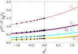
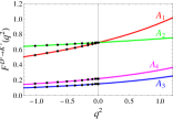
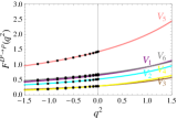
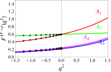
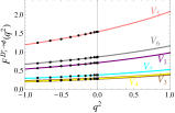
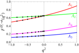
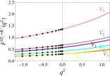
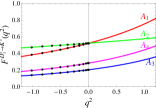
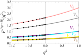
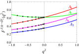
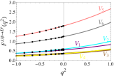
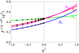
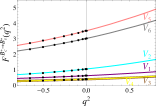
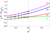
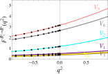
Figure 6: Same as Fig. 4 except with the parameterization scheme given by Eq. (74).

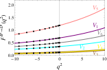
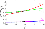
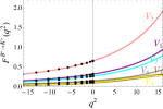
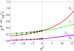
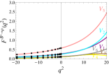
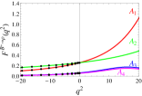
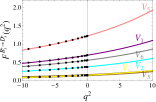
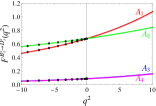
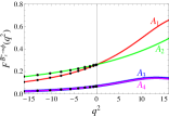
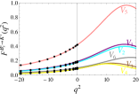
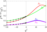
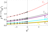
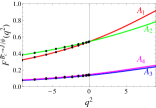
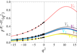
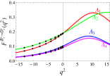
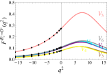
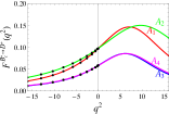
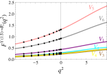
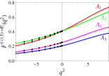
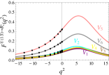
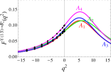
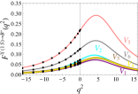
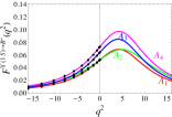
Table 8: Same as Table 4 except with the parameterization scheme given by Eq. (74). The errors are due to parameters $\beta$ and quark masses only (cf. section 4 for a more complete discussion).

	${\cal F}(0)$	$a$	$b$		${\cal F}(0)$	$a$	$b$
$V_{1}^{D^{*}\to\rho}$	$0.65_{-0.01-0.09}^{+0.01+0.09}$	$1.27_{-0.01-0.23}^{+0.00+0.31}$	$0.32_{-0.01-0.07}^{+0.00+0.09}$	$V_{1}^{D^{*}\to K^{*}}$	$0.74_{-0.02-0.10}^{+0.01+0.09}$	$1.28_{-0.01-0.31}^{+0.01+0.36}$	$0.34_{-0.01-0.15}^{+0.00+0.17}$
$V_{2}^{D^{*}\to\rho}$	$0.51_{-0.02-0.04}^{+0.02+0.03}$	$1.37_{-0.02-0.29}^{+0.01+0.31}$	$0.34_{-0.02-0.08}^{+0.01+0.11}$	$V_{2}^{D^{*}\to K^{*}}$	$0.43_{-0.03-0.08}^{+0.03+0.03}$	$1.33_{-0.03-0.26}^{+0.03+0.28}$	$0.33_{-0.02-0.12}^{+0.02+0.15}$
$V_{3}^{D^{*}\to\rho}$	$0.29_{-0.00-0.03}^{+0.00+0.03}$	$1.54_{-0.03-0.24}^{+0.03+0.36}$	$0.60_{-0.04-0.13}^{+0.04+0.25}$	$V_{3}^{D^{*}\to K^{*}}$	$0.26_{-0.00-0.02}^{+0.00+0.02}$	$1.54_{-0.03-0.33}^{+0.03+0.37}$	$0.62_{-0.04-0.12}^{+0.04+0.17}$
$V_{4}^{D^{*}\to\rho}$	$0.29_{-0.00-0.03}^{+0.00+0.03}$	$1.94_{-0.04-0.46}^{+0.04+0.66}$	$1.28_{-0.08-0.44}^{+0.08+0.72}$	$V_{4}^{D^{*}\to K^{*}}$	$0.26_{-0.00-0.02}^{+0.00+0.02}$	$1.77_{-0.03-0.31}^{+0.03+0.38}$	$0.91_{-0.05-0.37}^{+0.03+0.54}$
$V_{5}^{D^{*}\to\rho}$	$1.42_{-0.02-0.17}^{+0.02+0.17}$	$1.21_{-0.01-0.20}^{+0.01+0.30}$	$0.26_{-0.01-0.04}^{+0.00+0.05}$	$V_{5}^{D^{*}\to K^{*}}$	$1.50_{-0.03-0.16}^{+0.02+0.12}$	$1.23_{-0.01-0.18}^{+0.01+0.22}$	$0.28_{-0.01-0.04}^{+0.01+0.05}$
$V_{6}^{D^{*}\to\rho}$	$0.68_{-0.01-0.17}^{+0.01+0.17}$	$1.13_{-0.01-0.25}^{+0.01+0.35}$	$0.24_{-0.01-0.09}^{+0.00+0.15}$	$V_{6}^{D^{*}\to K^{*}}$	$0.78_{-0.02-0.17}^{+0.02+0.23}$	$1.19_{-0.02-0.24}^{+0.02+0.33}$	$0.27_{-0.01-0.10}^{+0.00+0.16}$
$A_{1}^{D^{*}\to\rho}$	$0.59_{-0.01-0.07}^{+0.01+0.07}$	$1.08_{-0.01-0.19}^{+0.00+0.27}$	$0.22_{-0.01-0.04}^{+0.01+0.06}$	$A_{1}^{D^{*}\to K^{*}}$	$0.69_{-0.01-0.09}^{+0.01+0.08}$	$1.11_{-0.01-0.17}^{+0.00+0.21}$	$0.24_{-0.00-0.03}^{+0.01+0.04}$
$A_{2}^{D^{*}\to\rho}$	$0.59_{-0.01-0.07}^{+0.01+0.07}$	$0.15_{-0.03-0.05}^{+0.03+0.05}$	$0.04_{-0.01-0.02}^{+0.00+0.02}$	$A_{2}^{D^{*}\to K^{*}}$	$0.69_{-0.01-0.09}^{+0.01+0.08}$	$0.26_{-0.05-0.05}^{+0.04+0.03}$	$0.02_{-0.01-0.00}^{+0.01+0.01}$
$A_{3}^{D^{*}\to\rho}$	$0.22_{-0.01-0.03}^{+0.01+0.03}$	$1.52_{-0.02-0.36}^{+0.02+0.43}$	$0.62_{-0.04-0.25}^{+0.03+0.45}$	$A_{3}^{D^{*}\to K^{*}}$	$0.15_{-0.01-0.04}^{+0.01+0.02}$	$1.48_{-0.05-0.21}^{+0.04+0.18}$	$0.59_{-0.04-0.06}^{+0.04+0.05}$
$A_{4}^{D^{*}\to\rho}$	$0.24_{-0.01-0.04}^{+0.01+0.06}$	$1.47_{-0.03-0.34}^{+0.03+0.51}$	$0.58_{-0.02-0.21}^{+0.04+0.42}$	$A_{4}^{D^{*}\to K^{*}}$	$0.22_{-0.01-0.03}^{+0.01+0.05}$	$1.47_{-0.03-0.30}^{+0.03+0.39}$	$0.61_{-0.04-0.33}^{+0.04+0.40}$
$V_{1}^{D_{s}^{*}\to K^{*}}$	$0.58_{-0.02-0.09}^{+0.02+0.10}$	$1.31_{-0.02-0.17}^{+0.01+0.19}$	$0.41_{-0.02-0.05}^{+0.02+0.05}$	$V_{1}^{D_{s}^{*}\to\phi}$	$0.71_{-0.01-0.10}^{+0.01+0.09}$	$1.35_{-0.00-0.19}^{+0.01+0.28}$	$0.45_{-0.01-0.07}^{+0.00+0.03}$
$V_{2}^{D_{s}^{*}\to K^{*}}$	$0.42_{-0.04-0.03}^{+0.04+0.02}$	$1.32_{-0.06-0.03}^{+0.05+0.01}$	$0.38_{-0.04-0.05}^{+0.04+0.05}$	$V_{2}^{D_{s}^{*}\to\phi}$	$0.38_{-0.03-0.11}^{+0.03+0.04}$	$1.41_{-0.04-0.24}^{+0.03+0.34}$	$0.43_{-0.03-0.03}^{+0.03+0.04}$
$V_{3}^{D_{s}^{*}\to K^{*}}$	$0.30_{-0.01-0.03}^{+0.00+0.03}$	$1.43_{-0.05-0.31}^{+0.04+0.43}$	$0.54_{-0.04-0.19}^{+0.04+0.26}$	$V_{3}^{D_{s}^{*}\to\phi}$	$0.28_{-0.00-0.02}^{+0.00+0.02}$	$1.48_{-0.04-0.33}^{+0.03+0.46}$	$0.57_{-0.04-0.20}^{+0.03+0.26}$
$V_{4}^{D_{s}^{*}\to K^{*}}$	$0.30_{-0.01-0.03}^{+0.00+0.03}$	$1.58_{-0.10-0.37}^{+0.09+0.40}$	$0.65_{-0.12-0.24}^{+0.14+0.33}$	$V_{4}^{D_{s}^{*}\to\phi}$	$0.28_{-0.00-0.02}^{+0.00+0.02}$	$1.71_{-0.09-0.40}^{+0.08+0.48}$	$0.77_{-0.13-0.29}^{+0.16+0.31}$
$V_{5}^{D_{s}^{*}\to K^{*}}$	$1.36_{-0.04-0.20}^{+0.04+0.19}$	$1.23_{-0.02-0.24}^{+0.02+0.28}$	$0.33_{-0.02-0.12}^{+0.02+0.17}$	$V_{5}^{D_{s}^{*}\to\phi}$	$1.54_{-0.03-0.16}^{+0.02+0.16}$	$1.27_{-0.01-0.18}^{+0.01+0.23}$	$0.35_{-0.01-0.04}^{+0.01+0.02}$
$V_{6}^{D_{s}^{*}\to K^{*}}$	$0.68_{-0.03-0.15}^{+0.03+0.21}$	$1.21_{-0.01-0.26}^{+0.01+0.33}$	$0.31_{-0.01-0.12}^{+0.02+0.21}$	$V_{6}^{D_{s}^{*}\to\phi}$	$0.86_{-0.02-0.19}^{+0.02+0.25}$	$1.23_{-0.01-0.28}^{+0.01+0.39}$	$0.34_{-0.01-0.14}^{+0.00+0.23}$
$A_{1}^{D_{s}^{*}\to K^{*}}$	$0.52_{-0.02-0.08}^{+0.02+0.07}$	$1.13_{-0.01-0.14}^{+0.01+0.17}$	$0.30_{-0.01-0.03}^{+0.01+0.03}$	$A_{1}^{D_{s}^{*}\to\phi}$	$0.65_{-0.01-0.09}^{+0.01+0.08}$	$1.16_{-0.01-0.17}^{+0.00+0.23}$	$0.32_{-0.01-0.05}^{+0.00+0.04}$
$A_{2}^{D_{s}^{*}\to K^{*}}$	$0.52_{-0.02-0.08}^{+0.02+0.08}$	$0.31_{-0.03-0.08}^{+0.02+0.06}$	$-0.06_{-0.00-0.02}^{+0.01+0.04}$	$A_{2}^{D_{s}^{*}\to\phi}$	$0.65_{-0.01-0.09}^{+0.01+0.08}$	$0.33_{-0.04-0.05}^{+0.04+0.04}$	$0.04_{-0.01-0.03}^{+0.00+0.02}$
$A_{3}^{D_{s}^{*}\to K^{*}}$	$0.20_{-0.02-0.03}^{+0.02+0.03}$	$1.35_{-0.07-0.09}^{+0.06+0.09}$	$0.49_{-0.06-0.07}^{+0.05+0.07}$	$A_{3}^{D_{s}^{*}\to\phi}$	$0.16_{-0.01-0.05}^{+0.01+0.02}$	$1.44_{-0.05-0.33}^{+0.04+0.40}$	$0.55_{-0.05-0.20}^{+0.05+0.32}$
$A_{4}^{D_{s}^{*}\to K^{*}}$	$0.28_{-0.01-0.05}^{+0.01+0.04}$	$1.37_{-0.05-0.31}^{+0.04+0.42}$	$0.51_{-0.03-0.18}^{+0.05+0.23}$	$A_{4}^{D_{s}^{*}\to\phi}$	$0.27_{-0.01-0.04}^{+0.01+0.05}$	$1.41_{-0.05-0.22}^{+0.04+0.24}$	$0.55_{-0.06-0.11}^{+0.06+0.12}$
$V_{1}^{J/\psi\to D^{*}}$	$0.55_{-0.02-0.12}^{+0.02+0.12}$	$1.61_{-0.04-0.13}^{+0.03+0.18}$	$0.96_{-0.03-0.02}^{+0.05+0.02}$	$V_{1}^{J/\psi\to D_{s}^{*}}$	$0.72_{-0.02-0.13}^{+0.01+0.12}$	$1.44_{-0.05-0.11}^{+0.05+0.13}$	$0.71_{-0.07-0.03}^{+0.07+0.03}$
$V_{2}^{J/\psi\to D^{*}}$	$0.60_{-0.05-0.10}^{+0.05+0.15}$	$1.93_{-0.04-0.45}^{+0.03+0.60}$	$1.28_{-0.02-0.63}^{+0.03+0.82}$	$V_{2}^{J/\psi\to D_{s}^{*}}$	$0.68_{-0.06-0.11}^{+0.06+0.14}$	$1.76_{-0.04-0.50}^{+0.03+0.50}$	$1.01_{-0.04-0.50}^{+0.03+0.66}$
$V_{3}^{J/\psi\to D^{*}}$	$0.36_{-0.01-0.03}^{+0.01+0.03}$	$1.68_{-0.04-0.40}^{+0.04+0.51}$	$0.91_{-0.06-0.36}^{+0.07+0.44}$	$V_{3}^{J/\psi\to D_{s}^{*}}$	$0.36_{-0.00-0.02}^{+0.00+0.01}$	$1.64_{-0.03-0.40}^{+0.03+0.56}$	$0.83_{-0.04-0.35}^{+0.04+0.46}$
$V_{4}^{J/\psi\to D^{*}}$	$0.36_{-0.01-0.03}^{+0.01+0.03}$	$1.90_{-0.03-0.43}^{+0.03+0.47}$	$1.18_{-0.05-0.46}^{+0.05+0.55}$	$V_{4}^{J/\psi\to D_{s}^{*}}$	$0.36_{-0.00-0.02}^{+0.00+0.01}$	$1.91_{-0.02-0.46}^{+0.02+0.56}$	$1.24_{-0.01-0.48}^{+0.01+0.57}$
$V_{5}^{J/\psi\to D^{*}}$	$1.79_{-0.05-0.34}^{+0.05+0.52}$	$1.54_{-0.03-0.37}^{+0.03+0.46}$	$0.82_{-0.03-0.36}^{+0.03+0.44}$	$V_{5}^{J/\psi\to D_{s}^{*}}$	$2.16_{-0.04-0.36}^{+0.04+0.51}$	$1.39_{-0.04-0.32}^{+0.03+0.38}$	$0.61_{-0.03-0.26}^{+0.03+0.38}$
$V_{6}^{J/\psi\to D^{*}}$	$1.23_{-0.05-0.34}^{+0.04+0.53}$	$1.61_{-0.08-0.48}^{+0.08+0.36}$	$0.45_{-0.33-0.40}^{+0.31+0.41}$	$V_{6}^{J/\psi\to D_{s}^{*}}$	$1.58_{-0.04-0.40}^{+0.04+0.58}$	$1.32_{-0.05-0.33}^{+0.04+0.40}$	$0.59_{-0.05-0.27}^{+0.04+0.39}$
$A_{1}^{J/\psi\to D^{*}}$	$0.47_{-0.01-0.09}^{+0.01+0.09}$	$1.39_{-0.03-0.12}^{+0.02+0.16}$	$0.71_{-0.04-0.02}^{+0.03+0.02}$	$A_{1}^{J/\psi\to D_{s}^{*}}$	$0.62_{-0.01-0.10}^{+0.01+0.08}$	$1.25_{-0.03-0.19}^{+0.03+0.12}$	$0.53_{-0.03-0.02}^{+0.03+0.02}$
$A_{2}^{J/\psi\to D^{*}}$	$0.47_{-0.01-0.09}^{+0.01+0.09}$	$0.38_{-0.08-0.23}^{+0.07+0.16}$	$-0.07_{-0.05-0.05}^{+0.05+0.06}$	$A_{2}^{J/\psi\to D_{s}^{*}}$	$0.62_{-0.01-0.10}^{+0.01+0.08}$	$0.90_{-0.08-0.35}^{+0.08+0.34}$	$-1.75_{-0.48-0.76}^{+0.50+0.72}$
$A_{3}^{J/\psi\to D^{*}}$	$0.38_{-0.01-0.08}^{+0.01+0.11}$	$1.69_{-0.01-0.43}^{+0.01+0.61}$	$0.95_{-0.00-0.40}^{+0.01+0.61}$	$A_{3}^{J/\psi\to D_{s}^{*}}$	$0.35_{-0.01-0.06}^{+0.01+0.07}$	$1.66_{-0.02-0.41}^{+0.01+0.55}$	$0.88_{-0.03-0.50}^{+0.03+0.68}$
$A_{4}^{J/\psi\to D^{*}}$	$0.45_{-0.01-0.11}^{+0.01+0.15}$	$1.59_{-0.03-0.39}^{+0.03+0.56}$	$0.85_{-0.04-0.35}^{+0.05+0.56}$	$A_{4}^{J/\psi\to D_{s}^{*}}$	$0.45_{-0.01-0.09}^{+0.01+0.13}$	$1.55_{-0.03-0.40}^{+0.03+0.57}$	$0.77_{-0.03-0.33}^{+0.05+0.46}$
$V_{1}^{B_{c}^{*}\to B^{*}}$	$0.52_{-0.02-0.11}^{+0.02+0.11}$	$1.85_{-0.03-0.18}^{+0.02+0.24}$	$1.56_{-0.03-0.19}^{+0.02+0.21}$	$V_{1}^{B_{c}^{*}\to B_{s}^{*}}$	$0.63_{-0.01-0.12}^{+0.01+0.12}$	$1.61_{-0.01-0.16}^{+0.01+0.20}$	$1.12_{-0.01-0.13}^{+0.01+0.13}$
$V_{2}^{B_{c}^{*}\to B^{*}}$	$1.18_{-0.13-0.28}^{+0.13+0.30}$	$2.41_{-0.04-0.36}^{+0.03+0.43}$	$2.51_{-0.04-0.20}^{+0.04+0.31}$	$V_{2}^{B_{c}^{*}\to B_{s}^{*}}$	$1.06_{-0.11-0.40}^{+0.11+0.20}$	$2.15_{-0.02-0.35}^{+0.01+0.37}$	$1.88_{-0.01-0.39}^{+0.02+0.48}$
$V_{3}^{B_{c}^{*}\to B^{*}}$	$0.40_{-0.01-0.04}^{+0.01+0.03}$	$1.88_{-0.07-0.27}^{+0.07+0.26}$	$1.35_{-0.15-0.26}^{+0.16+0.27}$	$V_{3}^{B_{c}^{*}\to B_{s}^{*}}$	$0.40_{-0.00-0.03}^{+0.00+0.01}$	$1.69_{-0.05-0.25}^{+0.05+0.31}$	$1.02_{-0.03-0.29}^{+0.04+0.11}$
$V_{4}^{B_{c}^{*}\to B^{*}}$	$0.40_{-0.01-0.04}^{+0.01+0.03}$	$2.01_{-0.06-0.40}^{+0.07+0.37}$	$1.51_{-0.16-0.28}^{+0.17+0.22}$	$V_{4}^{B_{c}^{*}\to B_{s}^{*}}$	$0.40_{-0.00-0.03}^{+0.00+0.01}$	$1.79_{-0.06-0.24}^{+0.06+0.24}$	$1.14_{-0.11-0.22}^{+0.10+0.20}$
$V_{5}^{B_{c}^{*}\to B^{*}}$	$3.15_{-0.11-0.82}^{+0.10+1.12}$	$1.80_{-0.03-0.26}^{+0.02+0.33}$	$1.43_{-0.02-0.34}^{+0.02+0.41}$	$V_{5}^{B_{c}^{*}\to B_{s}^{*}}$	$3.52_{-0.06-0.87}^{+0.06+1.12}$	$1.57_{-0.01-0.22}^{+0.01+0.28}$	$1.04_{-0.02-0.25}^{+0.01+0.27}$
$V_{6}^{B_{c}^{*}\to B^{*}}$	$2.66_{-0.10-0.79}^{+0.10+1.11}$	$1.79_{-0.03-0.27}^{+0.02+0.35}$	$1.45_{-0.03-0.36}^{+0.03+0.34}$	$V_{6}^{B_{c}^{*}\to B_{s}^{*}}$	$3.02_{-0.06-0.85}^{+0.06+1.15}$	$1.55_{-0.01-0.23}^{+0.01+0.30}$	$1.05_{-0.01-0.20}^{+0.01+0.29}$
$A_{1}^{B_{c}^{*}\to B^{*}}$	$0.43_{-0.02-0.08}^{+0.01+0.07}$	$1.59_{-0.02-0.16}^{+0.02+0.21}$	$1.15_{-0.03-0.14}^{+0.02+0.15}$	$A_{1}^{B_{c}^{*}\to B_{s}^{*}}$	$0.53_{-0.01-0.09}^{+0.01+0.08}$	$1.61_{-0.01-0.06}^{+0.01+0.10}$	$1.12_{-0.01-0.13}^{+0.01+0.12}$
$A_{2}^{B_{c}^{*}\to B^{*}}$	$0.43_{-0.02-0.08}^{+0.01+0.07}$	$0.32_{-0.10-0.20}^{+0.11+0.26}$	$-0.05_{-0.04-0.09}^{+0.04+0.09}$	$A_{2}^{B_{c}^{*}\to B_{s}^{*}}$	$0.53_{-0.01-0.09}^{+0.01+0.08}$	$0.19_{-0.08-0.13}^{+0.08+0.13}$	$-0.74_{-0.15-0.35}^{+0.10+0.39}$
$A_{3}^{B_{c}^{*}\to B^{*}}$	$0.81_{-0.03-0.20}^{+0.03+0.25}$	$1.93_{-0.02-0.35}^{+0.01+0.41}$	$1.44_{-0.06-0.37}^{+0.05+0.41}$	$A_{3}^{B_{c}^{*}\to B_{s}^{*}}$	$0.73_{-0.02-0.15}^{+0.02+0.16}$	$1.99_{-0.03-0.35}^{+0.03+0.50}$	$1.43_{-0.12-0.36}^{+0.10+0.38}$
$A_{4}^{B_{c}^{*}\to B^{*}}$	$0.89_{-0.02-0.24}^{+0.02+0.32}$	$1.86_{-0.07-0.34}^{+0.06+0.41}$	$1.35_{-0.12-0.35}^{+0.14+0.40}$	$A_{4}^{B_{c}^{*}\to B_{s}^{*}}$	$0.85_{-0.01-0.20}^{+0.01+0.25}$	$1.94_{-0.08-0.37}^{+0.05+0.47}$	$1.24_{-0.24-0.23}^{+0.20+0.33}$

Table 9: Same as Table 5 except with the parameterization scheme given by Eq. (74). The errors are due to parameters $\beta$ and quark masses only (cf. section 4 for a more complete discussion).

	${\cal F}(0)$	$a$	$b$		${\cal F}(0)$	$a$	$b$
$V_{1}^{B^{*}\to\rho}$	$0.27_{-0.01-0.04}^{+0.01+0.05}$	$1.58_{-0.02-0.11}^{+0.02+0.15}$	$0.72_{-0.04-0.02}^{+0.04+0.02}$	$V_{1}^{B^{*}\to K^{*}}$	$0.31_{-0.01-0.06}^{+0.01+0.06}$	$1.59_{-0.01-0.09}^{+0.01+0.10}$	$0.72_{-0.01-0.01}^{+0.01+0.01}$
$V_{2}^{B^{*}\to\rho}$	$0.25_{-0.01-0.03}^{+0.01+0.03}$	$1.70_{-0.10-0.23}^{+0.10+0.24}$	$0.78_{-0.06-0.07}^{+0.06+0.07}$	$V_{2}^{B^{*}\to K^{*}}$	$0.26_{-0.01-0.04}^{+0.01+0.03}$	$1.59_{-0.00-0.08}^{+0.01+0.08}$	$0.71_{-0.01-0.01}^{+0.01+0.01}$
$V_{3}^{B^{*}\to\rho}$	$0.10_{-0.00-0.01}^{-0.00+0.02}$	$2.00_{-0.03-0.17}^{+0.03+0.22}$	$1.60_{-0.07-0.18}^{+0.07+0.25}$	$V_{3}^{B^{*}\to K^{*}}$	$0.11_{-0.00-0.02}^{-0.00+0.02}$	$2.03_{-0.03-0.18}^{+0.02+0.19}$	$1.58_{-0.06-0.13}^{+0.07+0.12}$
$V_{4}^{B^{*}\to\rho}$	$0.10_{-0.00-0.01}^{+0.00+0.02}$	$2.23_{-0.05-0.23}^{+0.04+0.14}$	$2.33_{-0.09-0.19}^{+0.11+0.22}$	$V_{4}^{B^{*}\to K^{*}}$	$0.11_{-0.00-0.02}^{+0.00+0.02}$	$2.17_{-0.03-0.15}^{+0.03+0.19}$	$1.92_{-0.08-0.08}^{+0.08+0.14}$
$V_{5}^{B^{*}\to\rho}$	$0.57_{-0.01-0.09}^{+0.01+0.10}$	$1.55_{-0.03-0.11}^{+0.03+0.14}$	$0.68_{-0.04-0.01}^{+0.04+0.01}$	$V_{5}^{B^{*}\to K^{*}}$	$0.65_{-0.02-0.11}^{+0.02+0.11}$	$1.57_{-0.04-0.10}^{+0.03+0.12}$	$0.69_{-0.05-0.01}^{+0.04+0.01}$
$V_{6}^{B^{*}\to\rho}$	$0.12_{-0.00-0.02}^{+0.00+0.03}$	$1.50_{-0.02-0.12}^{+0.02+0.16}$	$0.60_{-0.03-0.02}^{+0.03+0.04}$	$V_{6}^{B^{*}\to K^{*}}$	$0.15_{-0.01-0.03}^{+0.01+0.04}$	$1.53_{-0.03-0.11}^{+0.03+0.13}$	$0.62_{-0.04-0.01}^{+0.04+0.03}$
$A_{1}^{B^{*}\to\rho}$	$0.26_{-0.01-0.04}^{+0.01+0.05}$	$1.57_{-0.02-0.11}^{+0.02+0.15}$	$0.71_{-0.05-0.01}^{+0.04+0.02}$	$A_{1}^{B^{*}\to K^{*}}$	$0.31_{-0.01-0.06}^{+0.01+0.06}$	$1.58_{-0.01-0.10}^{+0.01+0.13}$	$0.72_{-0.02-0.01}^{+0.01+0.01}$
$A_{2}^{B^{*}\to\rho}$	$0.26_{-0.01-0.04}^{+0.01+0.05}$	$0.70_{-0.01-0.01}^{+0.00+0.01}$	$0.08_{-0.01-0.04}^{+0.01+0.03}$	$A_{2}^{B^{*}\to K^{*}}$	$0.31_{-0.01-0.06}^{+0.01+0.06}$	$0.75_{-0.01-0.01}^{+0.01+0.01}$	$0.08_{-0.01-0.04}^{+0.01+0.04}$
$A_{3}^{B^{*}\to\rho}$	$0.07_{-0.00-0.01}^{+0.00+0.01}$	$2.13_{-0.00-0.22}^{+0.01+0.27}$	$1.83_{-0.01-0.26}^{+0.02+0.36}$	$A_{3}^{B^{*}\to K^{*}}$	$0.06_{-0.00-0.01}^{+0.00+0.01}$	$2.13_{-0.02-0.22}^{+0.02+0.25}$	$1.76_{-0.04-0.27}^{+0.06+0.34}$
$A_{4}^{B^{*}\to\rho}$	$0.06_{-0.00-0.01}^{+0.00+0.01}$	$2.12_{-0.03-0.20}^{+0.03+0.24}$	$1.83_{-0.08-0.23}^{+0.09+0.32}$	$A_{4}^{B^{*}\to K^{*}}$	$0.07_{-0.00-0.01}^{+0.00+0.01}$	$2.14_{-0.03-0.17}^{+0.04+0.23}$	$1.80_{-0.08-0.20}^{+0.08+0.27}$
$V_{1}^{B^{*}\to D^{*}}$	$0.70_{-0.01-0.11}^{+0.01+0.10}$	$1.57_{-0.01-0.03}^{+0.01+0.04}$	$0.58_{-0.01-0.02}^{+0.01+0.04}$	$V_{1}^{B_{s}^{*}\to K^{*}}$	$0.19_{-0.01-0.05}^{+0.01+0.06}$	$1.95_{-0.05-0.09}^{+0.05+0.10}$	$1.71_{-0.16-0.04}^{+0.16+0.04}$
$V_{2}^{B^{*}\to D^{*}}$	$0.35_{-0.01-0.04}^{+0.01+0.02}$	$1.58_{-0.02-0.10}^{+0.02+0.09}$	$0.57_{-0.05-0.10}^{+0.04+0.12}$	$V_{2}^{B_{s}^{*}\to K^{*}}$	$0.18_{-0.01-0.04}^{+0.01+0.04}$	$1.96_{-0.05-0.08}^{+0.04+0.10}$	$1.72_{-0.16-0.04}^{+0.15+0.05}$
$V_{3}^{B^{*}\to D^{*}}$	$0.12_{-0.00-0.01}^{+0.00+0.02}$	$2.09_{-0.02-0.33}^{+0.02+0.29}$	$1.45_{-0.05-0.44}^{+0.04+0.56}$	$V_{3}^{B_{s}^{*}\to K^{*}}$	$0.09_{-0.01-0.02}^{+0.01+0.02}$	$2.26_{-0.04-0.13}^{+0.04+0.16}$	$2.70_{-0.18-0.11}^{+0.20+0.14}$
$V_{4}^{B^{*}\to D^{*}}$	$0.12_{-0.00-0.01}^{+0.00+0.02}$	$2.21_{-0.02-0.42}^{+0.02+0.43}$	$1.65_{-0.03-0.34}^{+0.03+0.33}$	$V_{4}^{B_{s}^{*}\to K^{*}}$	$0.09_{-0.01-0.02}^{+0.01+0.02}$	$2.45_{-0.03-0.15}^{+0.03+0.17}$	$3.42_{-0.17-0.11}^{+0.17+0.13}$
$V_{5}^{B^{*}\to D^{*}}$	$1.19_{-0.01-0.14}^{+0.01+0.09}$	$1.56_{-0.02-0.04}^{+0.02+0.04}$	$0.55_{-0.02-0.02}^{+0.03+0.04}$	$V_{5}^{B_{s}^{*}\to K^{*}}$	$0.42_{-0.03-0.10}^{+0.02+0.12}$	$1.91_{-0.06-0.09}^{+0.05+0.09}$	$1.61_{-0.13-0.05}^{+0.14+0.04}$
$V_{6}^{B^{*}\to D^{*}}$	$0.51_{-0.01-0.13}^{+0.01+0.15}$	$1.56_{-0.03-0.06}^{+0.02+0.05}$	$0.54_{-0.02-0.02}^{+0.03+0.03}$	$V_{6}^{B_{s}^{*}\to K^{*}}$	$0.10_{-0.01-0.03}^{+0.01+0.03}$	$1.83_{-0.05-0.09}^{+0.04+0.10}$	$1.42_{-0.13-0.04}^{+0.13+0.03}$
$A_{1}^{B^{*}\to D^{*}}$	$0.69_{-0.01-0.11}^{+0.01+0.10}$	$1.57_{-0.01-0.03}^{+0.01+0.04}$	$0.57_{-0.01-0.03}^{+0.01+0.04}$	$A_{1}^{B_{s}^{*}\to K^{*}}$	$0.19_{-0.01-0.05}^{+0.01+0.05}$	$1.91_{-0.02-0.08}^{+0.03+0.10}$	$1.64_{-0.09-0.04}^{+0.09+0.04}$
$A_{2}^{B^{*}\to D^{*}}$	$0.69_{-0.01-0.11}^{+0.01+0.10}$	$0.75_{-0.02-0.01}^{+0.01+0.01}$	$-0.01_{-0.01-0.04}^{+0.00+0.04}$	$A_{2}^{B_{s}^{*}\to K^{*}}$	$0.19_{-0.01-0.05}^{+0.01+0.05}$	$1.11_{-0.06-0.03}^{+0.05+0.02}$	$0.48_{-0.06-0.11}^{+0.07+0.10}$
$A_{3}^{B^{*}\to D^{*}}$	$0.07_{-0.00-0.01}^{+0.00+0.01}$	$2.18_{-0.03-0.37}^{+0.02+0.37}$	$1.57_{-0.05-0.50}^{+0.04+0.57}$	$A_{3}^{B_{s}^{*}\to K^{*}}$	$0.06_{-0.00-0.01}^{+0.00+0.01}$	$2.34_{-0.10-0.16}^{+0.08+0.11}$	$2.94_{-0.12-0.19}^{+0.14+0.26}$
$A_{4}^{B^{*}\to D^{*}}$	$0.08_{-0.00-0.01}^{+0.00+0.01}$	$2.21_{-0.01-0.33}^{+0.00+0.36}$	$1.64_{-0.01-0.58}^{+0.01+0.54}$	$A_{4}^{B_{s}^{*}\to K^{*}}$	$0.05_{-0.00-0.01}^{+0.00+0.02}$	$2.33_{-0.05-0.15}^{+0.04+0.18}$	$2.90_{-0.19-0.16}^{+0.20+0.21}$
$V_{1}^{B_{s}^{*}\to\phi}$	$0.27_{-0.01-0.06}^{+0.01+0.07}$	$1.88_{-0.02-0.07}^{+0.02+0.09}$	$1.43_{-0.08-0.03}^{+0.08+0.02}$	$V_{1}^{B_{s}^{*}\to D_{s}^{*}}$	$0.69_{-0.01-0.12}^{+0.01+0.11}$	$1.65_{-0.03-0.01}^{+0.03+0.01}$	$0.82_{-0.06-0.09}^{+0.06+0.08}$
$V_{2}^{B_{s}^{*}\to\phi}$	$0.23_{-0.01-0.05}^{+0.01+0.05}$	$1.89_{-0.03-0.07}^{+0.03+0.09}$	$1.43_{-0.08-0.05}^{+0.08+0.05}$	$V_{2}^{B_{s}^{*}\to D_{s}^{*}}$	$0.38_{-0.01-0.03}^{+0.01+0.03}$	$1.71_{-0.01-0.19}^{+0.01+0.25}$	$0.85_{-0.01-0.12}^{+0.02+0.16}$
$V_{3}^{B_{s}^{*}\to\phi}$	$0.11_{-0.00-0.02}^{+0.00+0.02}$	$2.22_{-0.03-0.12}^{+0.03+0.14}$	$2.32_{-0.10-0.10}^{+0.10+0.13}$	$V_{3}^{B_{s}^{*}\to D_{s}^{*}}$	$0.15_{-0.00-0.02}^{+0.00+0.02}$	$2.11_{-0.03-0.36}^{+0.04+0.35}$	$1.59_{-0.07-0.54}^{+0.07+0.59}$
$V_{4}^{B_{s}^{*}\to\phi}$	$0.11_{-0.00-0.02}^{+0.00+0.02}$	$2.40_{-0.03-0.12}^{+0.03+0.13}$	$2.91_{-0.12-0.08}^{+0.11+0.06}$	$V_{4}^{B_{s}^{*}\to D_{s}^{*}}$	$0.15_{-0.00-0.02}^{+0.00+0.02}$	$2.41_{-0.01-0.43}^{+0.00+0.32}$	$2.38_{-0.01-0.47}^{+0.01+0.54}$
$V_{5}^{B_{s}^{*}\to\phi}$	$0.57_{-0.02-0.12}^{+0.02+0.14}$	$1.85_{-0.04-0.08}^{+0.03+0.08}$	$1.34_{-0.07-0.04}^{+0.08+0.03}$	$V_{5}^{B_{s}^{*}\to D_{s}^{*}}$	$1.22_{-0.02-0.16}^{+0.01+0.11}$	$1.64_{-0.04-0.01}^{+0.03+0.01}$	$0.78_{-0.05-0.08}^{+0.05+0.09}$
$V_{6}^{B_{s}^{*}\to\phi}$	$0.15_{-0.01-0.04}^{+0.01+0.05}$	$1.77_{-0.03-0.08}^{+0.03+0.10}$	$1.19_{-0.06-0.03}^{+0.06+0.03}$	$V_{6}^{B_{s}^{*}\to D_{s}^{*}}$	$0.55_{-0.01-0.14}^{+0.01+0.15}$	$1.58_{-0.04-0.03}^{+0.04+0.02}$	$0.72_{-0.05-0.05}^{+0.05+0.05}$
$A_{1}^{B_{s}^{*}\to\phi}$	$0.26_{-0.01-0.06}^{+0.01+0.07}$	$1.84_{-0.02-0.07}^{+0.03+0.09}$	$1.36_{-0.07-0.04}^{+0.08+0.03}$	$A_{1}^{B_{s}^{*}\to D_{s}^{*}}$	$0.68_{-0.01-0.12}^{+0.01+0.11}$	$1.65_{-0.04-0.01}^{+0.04+0.01}$	$0.81_{-0.05-0.09}^{+0.05+0.09}$
$A_{2}^{B_{s}^{*}\to\phi}$	$0.26_{-0.01-0.06}^{+0.01+0.07}$	$1.05_{-0.03-0.02}^{+0.03+0.03}$	$0.37_{-0.03-0.09}^{+0.03+0.08}$	$A_{2}^{B_{s}^{*}\to D_{s}^{*}}$	$0.68_{-0.01-0.12}^{+0.01+0.11}$	$0.80_{-0.05-0.05}^{+0.04+0.04}$	$0.13_{-0.02-0.08}^{+0.02+0.06}$
$A_{3}^{B_{s}^{*}\to\phi}$	$0.07_{-0.00-0.01}^{+0.00+0.01}$	$2.29_{-0.01-0.17}^{+0.00+0.23}$	$2.48_{-0.01-0.21}^{+0.00+0.29}$	$A_{3}^{B_{s}^{*}\to D_{s}^{*}}$	$0.09_{-0.00-0.01}^{+0.00+0.02}$	$2.21_{-0.00-0.37}^{+0.00+0.39}$	$1.76_{-0.01-0.50}^{+0.00+0.61}$
$A_{4}^{B_{s}^{*}\to\phi}$	$0.07_{-0.00-0.02}^{+0.00+0.02}$	$2.29_{-0.03-0.14}^{+0.03+0.17}$	$2.52_{-0.11-0.15}^{+0.11+0.18}$	$A_{4}^{B_{s}^{*}\to D_{s}^{*}}$	$0.09_{-0.00-0.01}^{+0.00+0.01}$	$2.22_{-0.03-0.38}^{+0.01+0.37}$	$1.75_{-0.01-0.57}^{+0.01+0.55}$

Table 10: Same as Table 6 except with the parameterization scheme given by Eq. (74). The errors are due to parameters $\beta$ and quark masses only (cf. section 4 for a more complete discussion).

	${\cal F}(0)$	$a$	$b$		${\cal F}(0)$	$a$	$b$
$V_{1}^{B_{c}^{*}\to D^{*}}$	$0.10_{-0.01-0.04}^{+0.01+0.06}$	$3.76_{-0.13-0.10}^{+0.12+0.09}$	$10.56_{-1.12-2.09}^{+1.18+1.97}$	$V_{1}^{B_{c}^{*}\to D_{s}^{*}}$	$0.20_{-0.02-0.07}^{+0.02+0.10}$	$2.42_{-0.09-0.06}^{+0.10+0.06}$	$3.43_{-0.39-0.62}^{+0.44+0.56}$
$V_{2}^{B_{c}^{*}\to D^{*}}$	$0.11_{-0.01-0.04}^{+0.01+0.06}$	$3.85_{-0.10-0.09}^{+0.10+0.08}$	$11.05_{-0.93-2.20}^{+1.02+2.05}$	$V_{2}^{B_{c}^{*}\to D_{s}^{*}}$	$0.20_{-0.02-0.06}^{+0.02+0.07}$	$2.51_{-0.10-0.05}^{+0.10+0.04}$	$3.15_{-0.29-0.35}^{+0.36+0.59}$
$V_{3}^{B_{c}^{*}\to D^{*}}$	$0.08_{-0.01-0.03}^{+0.01+0.04}$	$3.89_{-0.13-0.07}^{+0.13+0.06}$	$11.59_{-1.19-1.99}^{+1.25+1.87}$	$V_{3}^{B_{c}^{*}\to D_{s}^{*}}$	$0.13_{-0.01-0.04}^{+0.01+0.04}$	$2.57_{-0.09-0.03}^{+0.10+0.03}$	$4.00_{-0.43-0.59}^{+0.48+0.53}$
$V_{4}^{B_{c}^{*}\to D^{*}}$	$0.08_{-0.01-0.03}^{+0.01+0.04}$	$4.13_{-0.12-0.04}^{+0.12+0.03}$	$13.07_{-1.24-2.16}^{+1.33+2.01}$	$V_{4}^{B_{c}^{*}\to D_{s}^{*}}$	$0.13_{-0.01-0.04}^{+0.01+0.04}$	$2.76_{-0.04-0.05}^{+0.04+0.05}$	$5.02_{-0.52-0.54}^{+0.43+0.48}$
$V_{5}^{B_{c}^{*}\to D^{*}}$	$0.27_{-0.03-0.11}^{+0.03+0.15}$	$3.67_{-0.13-0.12}^{+0.13+0.10}$	$9.78_{-1.06-2.08}^{+1.12+1.99}$	$V_{5}^{B_{c}^{*}\to D_{s}^{*}}$	$0.50_{-0.05-0.16}^{+0.05+0.20}$	$2.36_{-0.09-0.06}^{+0.10+0.06}$	$3.19_{-0.37-0.57}^{+0.41+0.57}$
$V_{6}^{B_{c}^{*}\to D^{*}}$	$0.11_{-0.01-0.04}^{+0.01+0.06}$	$3.60_{-0.13-0.13}^{+0.13+0.11}$	$9.39_{-1.03-2.05}^{+1.09+2.02}$	$V_{6}^{B_{c}^{*}\to D_{s}^{*}}$	$0.22_{-0.02-0.07}^{+0.02+0.08}$	$2.28_{-0.10-0.08}^{+0.10+0.07}$	$2.96_{-0.35-0.50}^{+0.41+0.56}$
$A_{1}^{B_{c}^{*}\to D^{*}}$	$0.10_{-0.01-0.04}^{+0.01+0.06}$	$3.75_{-0.12-0.10}^{+0.13+0.08}$	$10.49_{-1.11-2.10}^{+1.15+1.98}$	$A_{1}^{B_{c}^{*}\to D_{s}^{*}}$	$0.19_{-0.02-0.06}^{+0.02+0.08}$	$2.37_{-0.09-0.06}^{+0.10+0.05}$	$3.28_{-0.36-0.60}^{+0.43+0.55}$
$A_{2}^{B_{c}^{*}\to D^{*}}$	$0.10_{-0.01-0.04}^{+0.01+0.06}$	$2.87_{-0.15-0.17}^{+0.14+0.19}$	$5.85_{-0.76-1.79}^{+0.79+1.83}$	$A_{2}^{B_{c}^{*}\to D_{s}^{*}}$	$0.19_{-0.02-0.06}^{+0.02+0.08}$	$1.65_{-0.10-0.17}^{+0.11+0.15}$	$1.58_{-0.24-0.49}^{+0.27+0.48}$
$A_{3}^{B_{c}^{*}\to D^{*}}$	$0.06_{-0.01-0.02}^{+0.01+0.03}$	$4.12_{-0.13-0.02}^{+0.13+0.02}$	$13.32_{-1.30-1.81}^{+1.37+1.78}$	$A_{3}^{B_{c}^{*}\to D_{s}^{*}}$	$0.10_{-0.01-0.03}^{+0.01+0.03}$	$2.68_{-0.09-0.02}^{+0.10+0.02}$	$4.43_{-0.45-0.59}^{+0.50+0.50}$
$A_{4}^{B_{c}^{*}\to D^{*}}$	$0.06_{-0.01-0.02}^{+0.01+0.03}$	$3.99_{-0.12-0.03}^{+0.13+0.03}$	$12.35_{-1.22-1.81}^{+1.29+1.78}$	$A_{4}^{B_{c}^{*}\to D_{s}^{*}}$	$0.09_{-0.01-0.03}^{+0.01+0.03}$	$2.61_{-0.09-0.01}^{+0.09+0.01}$	$4.17_{-0.42-0.52}^{+0.48+0.46}$
$V_{1}^{B_{c}^{*}\to J/\psi}$	$0.56_{-0.01-0.17}^{+0.01+0.17}$	$2.38_{-0.05-0.13}^{+0.05+0.16}$	$2.62_{-0.15-0.55}^{+0.15+0.61}$	$V_{1}^{\Upsilon(1S)\to B^{*}}$	$0.06_{-0.01-0.02}^{+0.01+0.03}$	$3.21_{-0.08-0.08}^{+0.08+0.09}$	$10.68_{-0.83-0.08}^{+0.81+0.06}$
$V_{2}^{B_{c}^{*}\to J/\psi}$	$0.33_{-0.01-0.04}^{+0.01+0.05}$	$2.45_{-0.02-0.02}^{+0.02+0.02}$	$2.76_{-0.07-0.29}^{+0.06+0.25}$	$V_{2}^{\Upsilon(1S)\to B^{*}}$	$0.08_{-0.01-0.03}^{+0.01+0.03}$	$3.39_{-0.05-0.11}^{+0.06+0.13}$	$11.98_{-0.92-0.23}^{+0.96+0.22}$
$V_{3}^{B_{c}^{*}\to J/\psi}$	$0.20_{-0.00-0.02}^{+0.00+0.02}$	$2.61_{-0.06-0.05}^{+0.06+0.05}$	$3.26_{-0.19-0.17}^{+0.20+0.17}$	$V_{3}^{\Upsilon(1S)\to B^{*}}$	$0.06_{-0.01-0.02}^{+0.01+0.03}$	$3.13_{-0.08-0.07}^{+0.08+0.07}$	$9.77_{-0.75-0.13}^{+0.83+0.08}$
$V_{4}^{B_{c}^{*}\to J/\psi}$	$0.20_{-0.00-0.02}^{+0.00+0.02}$	$2.84_{-0.07-0.09}^{+0.07+0.11}$	$4.06_{-0.27-0.16}^{+0.28+0.16}$	$V_{4}^{\Upsilon(1S)\to B^{*}}$	$0.06_{-0.01-0.02}^{+0.01+0.03}$	$3.22_{-0.07-0.08}^{+0.07+0.08}$	$10.11_{-0.75-0.16}^{+0.82+0.11}$
$V_{5}^{B_{c}^{*}\to J/\psi}$	$1.17_{-0.02-0.29}^{+0.02+0.23}$	$2.33_{-0.06-0.15}^{+0.05+0.17}$	$2.46_{-0.13-0.69}^{+0.15+0.60}$	$V_{5}^{\Upsilon(1S)\to B^{*}}$	$0.22_{-0.02-0.08}^{+0.03+0.11}$	$3.13_{-0.08-0.07}^{+0.08+0.08}$	$9.86_{-0.78-0.08}^{+0.76+0.05}$
$V_{6}^{B_{c}^{*}\to J/\psi}$	$0.65_{-0.01-0.19}^{+0.01+0.20}$	$2.45_{-0.25-0.31}^{+0.24+0.27}$	$2.28_{-0.13-0.59}^{+0.13+0.52}$	$V_{6}^{\Upsilon(1S)\to B^{*}}$	$0.13_{-0.02-0.05}^{+0.01+0.06}$	$3.15_{-0.08-0.07}^{+0.08+0.08}$	$10.18_{-0.82-0.03}^{+0.89+0.03}$
$A_{1}^{B_{c}^{*}\to J/\psi}$	$0.54_{-0.01-0.17}^{+0.01+0.16}$	$2.38_{-0.05-0.14}^{+0.05+0.16}$	$2.61_{-0.15-0.70}^{+0.15+0.61}$	$A_{1}^{\Upsilon(1S)\to B^{*}}$	$0.05_{-0.01-0.02}^{+0.01+0.03}$	$3.21_{-0.08-0.08}^{+0.08+0.09}$	$10.64_{-0.83-0.09}^{+0.91+0.06}$
$A_{2}^{B_{c}^{*}\to J/\psi}$	$0.54_{-0.01-0.17}^{+0.01+0.16}$	$1.59_{-0.05-0.19}^{+0.05+0.18}$	$1.09_{-0.07-0.48}^{+0.07+0.43}$	$A_{2}^{\Upsilon(1S)\to B^{*}}$	$0.05_{-0.01-0.02}^{+0.01+0.03}$	$2.75_{-0.10-0.03}^{+0.09+0.03}$	$7.91_{-0.73-0.16}^{+0.80+0.12}$
$A_{3}^{B_{c}^{*}\to J/\psi}$	$0.13_{-0.00-0.02}^{+0.00+0.03}$	$2.72_{-0.04-0.64}^{+0.03+0.72}$	$3.56_{-0.10-1.64}^{+0.08+1.72}$	$A_{3}^{\Upsilon(1S)\to B^{*}}$	$0.06_{-0.01-0.02}^{+0.01+0.03}$	$3.33_{-0.08-0.11}^{+0.07+0.12}$	$11.42_{-0.84-0.16}^{+0.92+0.14}$
$A_{4}^{B_{c}^{*}\to J/\psi}$	$0.14_{-0.00-0.02}^{+0.00+0.02}$	$2.72_{-0.06-0.06}^{+0.05+0.09}$	$3.57_{-0.19-0.09}^{+0.20+0.12}$	$A_{4}^{\Upsilon(1S)\to B^{*}}$	$0.07_{-0.01-0.03}^{+0.01+0.04}$	$3.22_{-0.07-0.09}^{+0.07+0.09}$	$10.45_{-0.77-0.03}^{+0.76+0.03}$
$V_{1}^{\Upsilon(1S)\to B_{s}^{*}}$	$0.09_{-0.01-0.03}^{+0.01+0.04}$	$3.26_{-0.06-0.08}^{+0.06+0.09}$	$9.04_{-0.51-0.09}^{+0.54+0.07}$	$V_{1}^{\Upsilon(1S)\to B_{c}^{*}}$	$0.44_{-0.01-0.13}^{+0.01+0.15}$	$3.16_{-0.09-0.04}^{+0.09+0.03}$	$5.36_{-0.35-0.17}^{+0.37+0.14}$
$V_{2}^{\Upsilon(1S)\to B_{s}^{*}}$	$0.11_{-0.01-0.03}^{+0.01+0.04}$	$3.46_{-0.02-0.11}^{+0.02+0.13}$	$10.23_{-0.14-0.22}^{+0.15+0.24}$	$V_{2}^{\Upsilon(1S)\to B_{c}^{*}}$	$0.29_{-0.03-0.05}^{+0.03+0.08}$	$3.38_{-0.04-0.46}^{+0.03+0.47}$	$6.08_{-0.14-1.85}^{+0.11+1.46}$
$V_{3}^{\Upsilon(1S)\to B_{s}^{*}}$	$0.09_{-0.01-0.03}^{+0.01+0.04}$	$3.19_{-0.06-0.07}^{+0.06+0.07}$	$8.36_{-0.47-0.06}^{+0.50+0.05}$	$V_{3}^{\Upsilon(1S)\to B_{c}^{*}}$	$0.24_{-0.01-0.04}^{+0.01+0.03}$	$3.18_{-0.07-0.14}^{+0.08+0.12}$	$5.33_{-0.31-0.34}^{+0.33+0.24}$
$V_{4}^{\Upsilon(1S)\to B_{s}^{*}}$	$0.09_{-0.01-0.03}^{+0.01+0.04}$	$3.43_{-0.21-0.22}^{+0.20+0.20}$	$9.47_{-1.27-0.70}^{+1.10+0.71}$	$V_{4}^{\Upsilon(1S)\to B_{c}^{*}}$	$0.24_{-0.01-0.04}^{+0.01+0.03}$	$3.29_{-0.06-0.12}^{+0.06+0.06}$	$5.63_{-0.28-0.97}^{+0.33+0.49}$
$V_{5}^{\Upsilon(1S)\to B_{s}^{*}}$	$0.32_{-0.02-0.11}^{+0.02+0.14}$	$3.18_{-0.06-0.07}^{+0.05+0.07}$	$8.36_{-0.48-0.06}^{+0.50+0.06}$	$V_{5}^{\Upsilon(1S)\to B_{c}^{*}}$	$1.31_{-0.04-0.33}^{+0.04+0.33}$	$3.08_{-0.07-0.05}^{+0.08+0.04}$	$5.00_{-0.33-0.13}^{+0.35+0.11}$
$V_{6}^{\Upsilon(1S)\to B_{s}^{*}}$	$0.19_{-0.01-0.06}^{+0.01+0.09}$	$3.19_{-0.06-0.07}^{+0.06+0.08}$	$8.57_{-0.49-0.19}^{+0.52+0.14}$	$V_{6}^{\Upsilon(1S)\to B_{c}^{*}}$	$0.92_{-0.03-0.25}^{+0.03+0.35}$	$3.06_{-0.09-0.34}^{+0.09+0.34}$	$4.97_{-0.27-1.14}^{+0.36+1.27}$
$A_{1}^{\Upsilon(1S)\to B_{s}^{*}}$	$0.08_{-0.01-0.03}^{+0.01+0.04}$	$3.25_{-0.05-0.08}^{+0.06+0.09}$	$9.01_{-0.50-0.09}^{+0.54+0.06}$	$A_{1}^{\Upsilon(1S)\to B_{c}^{*}}$	$0.41_{-0.01-0.12}^{+0.01+0.14}$	$3.16_{-0.09-0.04}^{+0.09+0.04}$	$5.35_{-0.34-0.16}^{+0.37+0.14}$
$A_{2}^{\Upsilon(1S)\to B_{s}^{*}}$	$0.08_{-0.01-0.03}^{+0.01+0.04}$	$2.77_{-0.07-0.03}^{+0.07+0.03}$	$6.56_{-0.43-0.09}^{+0.46+0.08}$	$A_{2}^{\Upsilon(1S)\to B_{c}^{*}}$	$0.41_{-0.01-0.12}^{+0.01+0.14}$	$3.46_{-0.11-0.05}^{+0.11+0.05}$	$3.21_{-0.32-0.07}^{+0.34+0.07}$
$A_{3}^{\Upsilon(1S)\to B_{s}^{*}}$	$0.09_{-0.01-0.03}^{+0.01+0.03}$	$3.39_{-0.05-0.09}^{+0.06+0.09}$	$9.75_{-0.52-0.08}^{+0.54+0.08}$	$A_{3}^{\Upsilon(1S)\to B_{c}^{*}}$	$0.21_{-0.01-0.04}^{+0.01+0.05}$	$3.35_{-0.02-0.49}^{+0.01+0.53}$	$5.95_{-0.06-1.69}^{+0.11+1.32}$
$A_{4}^{\Upsilon(1S)\to B_{s}^{*}}$	$0.10_{-0.01-0.03}^{+0.01+0.04}$	$3.28_{-0.05-0.08}^{+0.06+0.09}$	$8.97_{-0.50-0.04}^{+0.51+0.03}$	$A_{4}^{\Upsilon(1S)\to B_{c}^{*}}$	$0.25_{-0.01-0.04}^{+0.01+0.03}$	$3.30_{-0.08-0.29}^{+0.07+0.20}$	$5.76_{-0.32-1.08}^{+0.34+0.99}$

References

- [1] M. Wirbel, B. Stech and M. Bauer, Z. Phys. C 29 (1985) 637.
- [2] D. Daniel, R. Gupta and D. G. Richards, Phys. Rev. D 43 (1991) 3715.
- [3] L. Ametller, A. Bramon and E. Masso, Phys. Rev. D 48 (1993) 3388.
- [4] J. Gao and B. A. Li, Phys. Rev. D 61 (2000) 113006.
- [5] G. P. Lepage and S. J. Brodsky, Phys. Rev. D 22 (1980) 2157.
- [6] H. N. Li and G. F. Sterman, Nucl. Phys. B 381 (1992) 129.
- [7] M. A. Shifman, A. I. Vainshtein and V. I. Zakharov, Nucl. Phys. B 147 (1979) 385.
- [8] M. A. Shifman, A. I. Vainshtein and V. I. Zakharov, Nucl. Phys. B 147 (1979) 448.
- [9] M. V. Terentev, Sov. J. Nucl. Phys. 24 (1976) 106 [Yad. Fiz. 24 (1976) 207].
- [10] V. B. Berestetsky and M. V. Terentev, Sov. J. Nucl. Phys. 25 (1977) 347 [Yad. Fiz. 25 (1977) 653].
- [11] H. Y. Cheng, C. Y. Cheung, C. W. Hwang and W. M. Zhang, Phys. Rev. D 57 (1998) 5598.
- [12] J. Carbonell, B. Desplanques, V. A. Karmanov and J. F. Mathiot, Phys. Rept. 300 (1998) 215.
- [13] W. Jaus, Phys. Rev. D 60 (1999) 054026.
- [14] P. A. M. Dirac, Rev. Mod. Phys. 21 (1949) 392.
- [15] S. J. Brodsky, H. C. Pauli and S. S. Pinsky, Phys. Rept. 301 (1998) 299.
- [16] V. A. Karmanov and A. V. Smirnov, Nucl. Phys. A 546 (1992) 691.
- [17] V. A. Karmanov and A. V. Smirnov, Nucl. Phys. A 575 (1994) 520.
- [18] V. A. Karmanov and J. F. Mathiot, Nucl. Phys. A 602 (1996) 388.
- [19] H. M. Choi and C. R. Ji, Phys. Rev. D 58 (1998) 071901.
- [20] W. Jaus, Phys. Rev. D 41 (1990) 3394.
- [21] W. Jaus and D. Wyler, Phys. Rev. D 41 (1990) 3405.
- [22] C. Q. Geng, C. W. Hwang, C. C. Lih and W. M. Zhang, Phys. Rev. D 64 (2001) 114024.
- [23] C. Q. Geng, C. C. Lih and C. Xia, Eur. Phys. J. C 76 (2016) no.6, 313.
- [24] W. Jaus, Phys. Rev. D 44 (1991) 2851.
- [25] W. Jaus, Phys. Rev. D 53 (1996) 1349.
- [26] H. Y. Cheng, C. Y. Cheung and C. W. Hwang, Phys. Rev. D 55 (1997) 1559.
- [27] P. J. O’Donnell and G. Turan, Phys. Rev. D 56 (1997) 295.
- [28] C. Y. Cheung, C. W. Hwang and W. M. Zhang, Z. Phys. C 75 (1997) 657.
- [29] H. M. Choi and C. R. Ji, Nucl. Phys. A 618 (1997) 291.
- [30] H. M. Choi and C. R. Ji, Phys. Rev. D 59 (1999) 074015.
- [31] H. M. Choi and C. R. Ji, Phys. Rev. D 59 (1998) 034001.
- [32] C. R. Ji and H. M. Choi, Phys. Lett. B 513 (2001) 330.
- [33] M. A. DeWitt, H. M. Choi and C. R. Ji, Phys. Rev. D 68 (2003) 054026.
- [34] H. M. Choi and C. R. Ji, Phys. Rev. D 75 (2007) 034019.
- [35] H. M. Choi, Phys. Rev. D 75 (2007) 073016.
- [36] N. Barik, S. K. Tripathy, S. Kar and P. C. Dash, Phys. Rev. D 56 (1997) 4238.
- [37] C. W. Hwang, Eur. Phys. J. C 19 (2001) 105.
- [38] C. W. Hwang, Phys. Rev. D 81 (2010) 114024.
- [39] C. W. Hwang, Phys. Lett. B 516 (2001) 65.
- [40] C. W. Hwang, JHEP 0910 (2009) 074.
- [41] Q. Chang, S. J. Brodsky and X. Q. Li, Phys. Rev. D 95 (2017) no.9, 094025.
- [42] Q. Chang, S. Xu and L. Chen, Nucl. Phys. B 921 (2017) 454.
- [43] Q. Chang, X. N. Li, X. Q. Li and F. Su, Chin. Phys. C 42 (2018) no.7, 073102.
- [44] Q. Chang, L. L. Chen and S. Xu, J. Phys. G 45 (2018) no.7, 075005.
- [45] B. L. G. Bakker, H. M. Choi and C. R. Ji, Phys. Rev. D 63 (2001) 074014.
- [46] B. L. G. Bakker, H. M. Choi and C. R. Ji, Phys. Rev. D 65 (2002) 116001.
- [47] B. L. G. Bakker, H. M. Choi and C. R. Ji, Phys. Rev. D 67 (2003) 113007.
- [48] H. M. Choi and C. R. Ji, Phys. Rev. D 70 (2004) 053015.
- [49] H. M. Choi and C. R. Ji, Phys. Rev. D 80 (2009) 054016.
- [50] H. M. Choi and C. R. Ji, Phys. Rev. D 80 (2009) 114003.
- [51] H. M. Choi, Phys. Rev. D 81 (2010) 054003.
- [52] H. M. Choi, J. Phys. G 37 (2010) 085005.
- [53] H. M. Choi and C. R. Ji, Phys. Lett. B 696 (2011) 518.
- [54] H. M. Choi and C. R. Ji, Nucl. Phys. A 856 (2011) 95.
- [55] H. M. Choi and C. R. Ji, Phys. Rev. D 91 (2015) no.1, 014018.
- [56] H. M. Choi and C. R. Ji, Phys. Rev. D 95 (2017) no.5, 056002.
- [57] H. M. Choi, H. Y. Ryu and C. R. Ji, Phys. Rev. D 96 (2017) no.5, 056008.
- [58] H. Y. Ryu, H. M. Choi and C. R. Ji, Phys. Rev. D 98 (2018) no.3, 034018.
- [59] C. W. Hwang, Phys. Rev. D 64 (2001) 034011.
- [60] C. W. Hwang, Phys. Lett. B 530 (2002) 93.
- [61] C. W. Hwang and R. S. Guo, Phys. Rev. D 82 (2010) 034021.
- [62] C. Y. Cheung and C. W. Hwang, JHEP 1404 (2014) 177.
- [63] W. Wang and Y. L. Shen, Phys. Rev. D 78 (2008) 054002.
- [64] W. Wang, Y. L. Shen and C. D. Lu, Phys. Rev. D 79 (2009) 054012.
- [65] Y. L. Shen and Y. M. Wang, Phys. Rev. D 78 (2008) 074012.
- [66] X. X. Wang, W. Wang and C. D. Lu, Phys. Rev. D 79 (2009) 114018.
- [67] H. Y. Cheng and X. W. Kang, Eur. Phys. J. C 77 (2017) no.9, 587 Erratum: [Eur. Phys. J. C 77 (2017) no.12, 863].
- [68] X. W. Kang, T. Luo, Y. Zhang, L. Y. Dai and C. Wang, arXiv:1808.02432 [hep-ph].
- [69] W. Jaus, Phys. Rev. D 67 (2003) 094010.
- [70] H. Y. Cheng, C. K. Chua and C. W. Hwang, Phys. Rev. D 69 (2004) 074025.
- [71] R. C. Verma, J. Phys. G 39 (2012) 025005.
- [72] Y. J. Shi, W. Wang and Z. X. Zhao, Eur. Phys. J. C 76 (2016) no.10, 555.
- [73] W. Wang and R. Zhu, arXiv:1808.10830 [hep-ph].
- [74] H. Y. Cheng, C. K. Chua and C. W. Hwang, Phys. Rev. D 70 (2004) 034007.
- [75] H. Y. Cheng and C. K. Chua, JHEP 0411 (2004) 072.
- [76] Z. T. Wei, H. W. Ke and X. Q. Li, Phys. Rev. D 80 (2009) 094016.
- [77] W. Wang, F. S. Yu and Z. X. Zhao, Eur. Phys. J. C 77 (2017) no.11, 781.
- [78] H. W. Ke, N. Hao and X. Q. Li, arXiv:1711.02518 [hep-ph].
- [79] Z. X. Zhao, Chin. Phys. C 42 (2018) no.9, 093101.
- [80] Z. X. Zhao, Eur. Phys. J. C 78 (2018) no.9, 756.
- [81] C. K. Chua, Phys. Rev. D 99 (2019) no.1, 014023.
- [82] T. Abe et al. [Belle-II Collaboration], arXiv:1011.0352.
- [83] R. Aaij et al. [LHCb Collaboration], Eur. Phys. J. C 73 (2013) no.4, 2373.
- [84] R. Aaij et al. [LHCb Collaboration], Int. J. Mod. Phys. A 30 (2015) no.07, 1530022.
- [85] H. M. Choi and C. R. Ji, Phys. Rev. D 89 (2014) no. 3, 033011.
- [86] Q. Chang, X. N. Li, X. Q. Li, F. Su and Y. D. Yang, Phys. Rev. D 98 (2018) no.11, 114018.
- [87] Q. Chang, X. N. Li and L. T. Wang, Eur. Phys. J. C 79 (2019) no.5, 422.
- [88] Y. M. Wang, H. Zou, Z. T. Wei, X. Q. Li and C. D. Lu, Eur. Phys. J. C 54 (2008) 107.
- [89] H. M. Choi, C. R. Ji, Z. Li and H. Y. Ryu, Phys. Rev. C 92 (2015) no.5, 055203.
- [90] P. Ball and V. M. Braun, Phys. Rev. D 58 (1998) 094016.
- [91] C. Bourrely, B. Machet and E. de Rafael, Nucl. Phys. B 189 (1981) 157.
- [92] C. Bourrely, I. Caprini and L. Lellouch, Phys. Rev. D 79 (2009) 013008 Erratum: [Phys. Rev. D 82 (2010) 099902].
- [93] J. Gao, C. D. Lu, Y. L. Shen, Y. M. Wang and Y. B. Wei, arXiv:1907.11092 [hep-ph].
- [94] R. J. Dowdall, C. T. H. Davies, T. C. Hammant and R. R. Horgan, Phys. Rev. D 86 (2012) 094510.
- [95] T. Wang, Y. Jiang, T. Zhou, X. Z. Tan and G. L. Wang, J. Phys. G 45 (2018) no.11, 115001.
- [96] M. A. Ivanov and C. T. Tran, Phys. Rev. D 92 (2015) no.7, 074030.
- [97] T. Wang, Y. Jiang, H. Yuan, K. Chai and G. L. Wang, J. Phys. G 44 (2017) no.4, 045004.
- [98] G. P. Lepage, S. J. Brodsky, T. Huang, P. B. Mackenzie, in: A. Z. Capri, A. N. Kamal (Eds.), Particles and Fields 2, Plenum Press, New York, 1983.
- [99] C. Y. Cheung, W. M. Zhang and G. L. Lin, Phys. Rev. D 52 (1995) 2915.
- [100] H. M. Choi and C. R. Ji, Phys. Rev. D 56 (1997) 6010.
- [101] W. Jaus, Phys. Rev. D 63 (2001) 053009.