Spin-1/2 Ising-Heisenberg Cairo pentagonal model in the presence of an external magnetic field: Effect of Landé g-factors

Abstract

In the present paper, a study of the magnetic properties of a spin-1/2 Ising-Heisenberg Cairo pentagonal structure is presented. The model has been investigated in Ref. Rodrigues in the absence of external magnetic field. Here, we consider the effects of an external tunable magnetic field. By using the transfer matrix approach, we investigate the magnetic ground-state phase transition, the low-temperature magnetization process, and how the magnetic field influences the various thermodynamic parameters such as entropy, internal energy and specific heat. It is shown that the model exhibits intermediate magnetization plateaux accompanied by a double-peak in the specific heat curve versus temperature. The position of each magnetization jump is in accordance with the merging and/or separation of the two peaks in the specific heat curve. Considering different g-factors for the nodal Ising spins and spin dimers also results in arising different intermediate plateaux and to remarkable alterations of the thermodynamic properties of the model.

I Introduction

The study of quantum spin systems with competing interactions is an active field of research in solid state physics. Efforts have focused on ferrimagnetic chains, since they feature both ferromagnetic and antiferromagnetic phases, which have been studied both at zero and finite temperature Kitaev ; Gu ; Dillenschneider ; Ivanov ; Werlang ; Sachdev ; Rojas2 ; RojasM ; Strecka . Spin ladders have been also extensively studied using various methods Strecka ; Koga ; Okamoto ; Muller ; Vuletic ; Notbohm ; Buttner ; Blundell ; Bacq ; Arian1 ; Feng2007 ; Giuseppe2020 . Analogously, 2-D lattices like spin-1/2 Heisenberg antiferromagnets on the kagome lattice have been also widely examined within the Lanczos diagonalization both for the ground state properties up to $48$ spins Moessner2019 and at finite temperature up to $42$ spins Schnack2018 , and using DMRG White2011 ; Kolley2015 .

Along the years, the synthesis of compounds such as $\mathrm{A}_{3}\mathrm{Cu}_{3}(\mathrm{PO}_{4})_{4}$ with $\mathrm{A}=\mathrm{Ca},\mathrm{Sr}$ Drillon1 , $\mathrm{Cu}_{3}\mathrm{Cl}_{6}(\mathrm{H}_{2}\mathrm{O})_{2}\\ \cdot 2\mathrm{H}_{8}\mathrm{C}_{4}\mathrm{SO}_{2}$ Okamoto1999 ; Okamoto2003 , the diamond chain like polymers $\mathrm{Cu}_{3}(\mathrm{TeO}_{3})_{2}\mathrm{Br}_{2}$ Uematsu and the natural mineral azurite $[\mathrm{Cu}_{3}(\mathrm{CO}_{3})_{2}(\mathrm{OH})_{2}]$ Kikuchi1 ; Kikuchi2 , became possible. These materials can be studied in terms of Heisenberg spin models. Recently, a mixed $3d/4f$ cyclic coordination cluster with a ground-state spin of $S=60$ was studied experimentally in Baniodeh , where the authors synthesised the $\mathrm{Gd}$-containing isotropic member of a new series of cyclic coordination clusters, forming a nano-torus with alternating gadolinium and iron ions with a nearest neighbour $\mathrm{Fe}–\mathrm{Gd}$ coupling and a frustrating next-nearest neighbour $\mathrm{Fe}–\mathrm{Fe}$ coupling. This arrangement corresponds to a cyclic delta or saw-tooth chain Baniodeh . Motivated by the compound $\mathrm{Bi}_{2}\mathrm{Fe}_{4}\mathrm{O}_{9}$, in Ref. Rojas2012 it was given a general solution for the frustrated Ising model on the so-called 2-D Cairo pentagonal lattice, i.e. a planar lattice where the tiling is achieved with non-regular pentagons. In Ref. Rousochatzakis2012 the antiferromagnetic Heisenberg model on the Cairo pentagonal lattice was studied. Afterwards, F. C. Rodrigues et al. sketched a stripe of the Cairo pentagonal Ising-Heisenberg model, and studied the ground-state phase transition and some thermodynamic parameters for such model in Rodrigues . The advantage of the Cairo pentagonal Ising-Heisenberg stripe geometry is to make possible analytical calculations, and also the possibility of considering the effect of the interactions of classical spins interacting with quantum ones. Another advantage, exploited in the following, is that it allows for an evaluation of the effect of external magnetic fields.

Phase transitions in spin models with competing interactions has been one of the most interesting topics of condensed matter physics and statistical mechanics during the last decades Arian1 ; Feng2007 ; Saadatmand ; Valverde ; Ananikian2012 ; Abgaryan1 ; Strecka1 ; Arian2 ; Campa20 . Further investigations of the spin models in the presence of an external magnetic field have supplied exact outcomes for the ground-state phase transition, which can be induced through the exchange couplings Sahoo1 ; Sahoo2 ; Giri ; Hovhannisyan . The ground-state of the spin ladders with higher spins have been examined so far Ivanov ; Giri .

The investigation of magnetization curves and plateaux has attracted considerable interest. Exactly solvable quantum spin models for which magnetization varies smoothly as a function of the magnetic field until reaches its saturation magnetization include spin-1/2 quantum chains Hida ; Verkholyak , ladders Arian1 ; Cabra and spin-1/2 Ising-Heisenberg diamond chains Gu ; Rojas2 ; RojasM ; Ananikian2012 ; Abgaryan1 ; Strecka1 . The specific heat of magnetic materials has attracted as well much attention, since it may exhibit an anomalous thermal behavior when the parameters of the Hamiltonian such as coupling constants, spin exchange anisotropy and magnetic field are changed. Such a function can be estimated by the Schottky theory Strecka ; Karlova2016 . The associated round maximum (Schottky maximum) appeared in the specific heat curve, has been detected in various magnetic materials in experiments Bernu ; Misguich ; Helton .

When practicable, the possibility of using an analytical approach to describe the ground-state diagram and magnetic and thermodynamic properties of quantum spin systems such as magnetization, entropy, internal energy and specific heat, is certainly unvaluable. A very useful method is the transfer-matrix formalism which has widely been applied to a number of strongly correlated systems at zero-temperature and low temperature for studying the ground- and low-lying state properties of spin models. In the following of the analytical discussion in Ref. Rodrigues , we here investigate the magnetic and thermodynamic properties of the spin-1/2 Ising-Heisenberg Cairo pentagonal model in the presence of an external magnetic field using the same transfer matrix technique. We also consider the possibility to have in this model different Landé g-factors Vadim2015 ; Vadim2020 , showing that the diffence among them plays an important role in the magnetic and thermodynamic behaviors of the model.

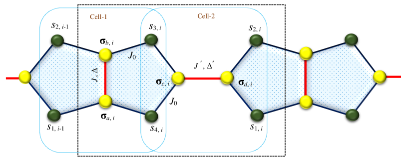
Figure 1: Schematic representation of the spin-1/2 Ising-Heisenberg Cairo pentagonal model. Yellow circles represent Heisenberg dimer spins and green circles between them, localized on the external vertices of each pentagon, represent the Ising nodal spins. The dashed rectangle represents an unit block.

The paper is organized as follows. In Sec. II we describe the model and present its thermodynamic solution with in the transfer-matrix formalism. In Sec. III, we numerically discuss the magnetization process and the thermodynamic behavior of the model in the presence of an external homogeneous magnetic field. Finally, the most significant results will be summarized together in Sec. IV.

II Model and exact solution within the transfear matrix formalism

The Hamiltonian of the spin-1/2 Ising-Heisenberg Cairo pentagonal model shown in Fig. 1 can be written as

$$\begin{array}[]{lcl}H=\sum\limits_{i=1}^{N}\big{[}\mathcal{H}_{i-1,i}^{ab}+\mathcal{H}_{i,i}^{cd}\big{]}+{H_{z}},\end{array}$$ (1)

where the Hamiltonians of two sub-units block cell-1 ($\mathcal{H}_{i-1,i}^{ab}$) and cell-2 ($\mathcal{H}_{i,i}^{cd}$) in each block together with the Zeeman term are given by

$$\begin{array}[]{lcl}\mathcal{H}_{i-1,i}^{ab}=-J({\bm{\sigma}}_{a,i}\cdot{\bm{\sigma}}_{b,i})_{\Delta}-J_{0}\big{(}s_{1,i-1}+s_{4,i}\big{)}{\sigma}_{a,i}^{z}-J_{0}\big{(}s_{2,i-1}+s_{3,i})\sigma_{b,i}^{z},\\ \mathcal{H}_{i,i}^{cd}=-J^{\prime}({\bm{\sigma}}_{c,i}\cdot{\bm{\sigma}}_{d,i})_{\Delta^{\prime}}-J_{0}\big{(}s_{3,i}+s_{4,i}\big{)}{\sigma}_{c,i}^{z}-J_{0}\big{(}s_{1,i}+s_{2,i})\sigma_{d,i}^{z},\\ H_{z}=-\mu_{B}B_{z}\sum\limits_{i=1}^{N}{\big{[}}g_{1}{\big{(}}\sigma_{a,i}^{z}+\sigma_{b,i}^{z}+\sigma_{c,i}^{z}+\sigma_{d,i}^{z}{\big{)}}+\dfrac{1}{2}g_{2}{\big{(}}s_{1,i}+s_{2,i}+s_{3,i}+s_{4,i}{\big{)}\big{]}},\end{array}$$ (2)

where $N$ is the number of unit blocks. Two different Landé g-factors $g_{1}$ and $g_{2}$ are considered. The XXZ interaction between pair spins of $ab$-dimer can be given by

$$\begin{array}[]{lcl}J({\bm{\sigma}}_{a,i}\cdot{\bm{\sigma}}_{b,i})_{\Delta}\equiv J\big{(}\sigma_{a,i}^{x}\sigma_{b,i}^{x}+\sigma_{a,i}^{y}\sigma_{b,i}^{y}\big{)}+\Delta\sigma_{a,i}^{z}\sigma_{b,i}^{z}.\end{array}$$ (3)

Analogously, for the $cd$-dimer we have following definition

$$\begin{array}[]{lcl}J^{\prime}({\bm{\sigma}}_{c,i}\cdot{\bm{\sigma}}_{d,i})_{\Delta^{\prime}}\equiv J^{\prime}\big{(}\sigma_{c,i}^{x}\sigma_{d,i}^{x}+\sigma_{c,i}^{y}\sigma_{d,i}^{y}\big{)}+\Delta^{\prime}\sigma_{c,i}^{z}\sigma_{d,i}^{z}.\end{array}$$ (4)

The nodal spins $s^{\alpha,i}$ ($\alpha=\{1,2,3,4\}$) localized on the wings of each pentagon are Pauli operators, taking values $(-1,\;1)$. The pure Ising-type exchange coupling $J_{0}$ represents interaction between nodal spins $s^{\alpha,i}$ and Heisenberg dimer spins. $\bm{\sigma}=\{{\sigma}^{x},{\sigma}^{y},{\sigma}^{z}\}$ are Pauli operators of Heisenberg dimers (with $\hbar=1$) and are given by

$$\sigma^{x}=\left(\begin{array}[]{cc}0&1\\ 1&0\end{array}\right),\quad\sigma^{y}=\left(\begin{array}[]{cc}0&-i\\ i&0\end{array}\right),\quad\sigma^{z}=\left(\begin{array}[]{cc}1&0\\ 0&-1\end{array}\right).$$

The final part of the Hamiltonian (1) accounts for the Zeeman^,s energy of magnetic moments in the external magnetic field $B={B}_{z}$. We will write $H_{z}=\sum_{i=1}^{N}\mathcal{H}^{i}_{z}$, with $\mathcal{H}^{i}_{z}=(\mathcal{H}_{i-1,i}^{ab})^{z}+(\mathcal{H}_{i,i}^{cd})^{z}$ representing the Zeeman^,s energy of each two cells in the block Hamiltonian, and $H=\sum_{i=1}^{N}\mathcal{H}_{i}$, with $\mathcal{H}_{i}=\mathcal{H}_{i-1,i}^{ab}+\mathcal{H}_{i,i}^{cd}+\mathcal{H}^{i}_{z}$. From now on, we consider $J_{0}$ as energy unit for all other parameters with $B/J_{0}$, $J/J_{0}$, $\Delta/J_{0}$ and $T/J_{0}$ being dimensionless parameters, restoring $J_{0}$ in equations and plots when needed for clarity. Moreover, we will set $\mu_{B}=1$.

The commutation relation between each of two different block Hamiltonians $[\mathcal{H}_{i},\mathcal{H}_{j}]=0$ enables us to extract the partition function of the model under consideration from the following formula

$${Z}=Tr\Big{[}\displaystyle\prod_{i=1}^{{N}}\exp\big{(}-\beta{\mathcal{H}_{i}}\big{)}\Big{]},$$ (5)

where $\beta=1/k_{B}T$ with $k_{B}$ the Boltzmann constant and $T$ the temperature (for simplicity we set $k_{B}=1$). Hence, we can write the $4\times 4$ transfer matrix $\mathcal{W}$ as it follows:

$$\begin{array}[]{lcl}\mathcal{W}=\mathcal{T}_{ab}\mathcal{T}_{cd}=\sum\limits_{k=1}^{4}\exp\big{[}-\beta\mathcal{E}_{k}(s_{1,i-1}\;s_{2,i-1}\mid s_{4,i}\;s_{3,i})\big{]}\sum\limits_{k=1}^{4}\exp\big{[}-\beta\bar{\mathcal{E}}_{k}(s_{1,i}\;s_{4,i}\mid s_{2,i}\;s_{3,i})\big{]}.\end{array}$$ (6)

$\mathcal{T}_{ab}$ represents the transfer matrix of the cell-1 and $\mathcal{T}_{cd}$ represents the transfer matrix of the cell-2. Symbol $\mid$ distinguishes the interplay between rows (pair nodal spins $\{s_{1,i-1},\;s_{2,i-1}\}$) and the columns (nodal spins $\{s_{4,i},\;s_{3,i}\}$) of the transfer matrix $\mathcal{T}_{ab}$, and between rows (pair nodal spins $\{s_{1,i},\;s_{4,i}\}$) and the columns (nodal spins $\{s_{2,i},\;s_{3,i}\}$) of the transfer matrix $\mathcal{T}_{cd}$. Moreover, $\mathcal{E}_{k}$ denote the eigenvalues of the Hamiltonian $\mathcal{H}_{i-1,i}^{ab}+(\mathcal{H}_{i-1,i}^{ab})^{z}$ and depend on the spins $s_{\alpha,i}$ (with $\alpha=1,2,3,4$). One obtains

$$\begin{array}[]{lcl}\mathcal{E}_{1,2}=-\frac{\Delta}{4}-\frac{g_{2}B}{4}(s_{1,i-1}+s_{2,i-1}+s_{3,i}+s_{4,i})\pm\frac{1}{4}\left(2g_{1}B+J(s_{1,i-1}+s_{2,i-1}+s_{3,i}+s_{4,i})\right),\\ \mathcal{E}_{3,4}=\frac{\Delta}{4}-\frac{g_{2}B}{4}(s_{1,i-1}+s_{2,i-1}+s_{3,i}+s_{4,i})\pm\frac{1}{2}\sqrt{J_{0}^{2}\left(s_{1,i-1}+s_{4,i}-s_{2,i-1}-s_{3,i}\right)^{2}+J^{2}}.\end{array}$$ (7)

Analogously, the corresponding eigenenergies for $cd$-dimer are given by

$$\begin{array}[]{lcl}\bar{\mathcal{E}}_{1,2}=-\frac{\Delta^{\prime}}{4}-\frac{g_{2}B}{4}(s_{1,i}+s_{2,i}+s_{3,i}+s_{4,i})\pm\frac{1}{4}\left(2g_{1}B+J^{\prime}(s_{1,i}+s_{2,i}+s_{3,i}+s_{4,i})\right),\\ \bar{\mathcal{E}}_{3,4}=\frac{\Delta^{\prime}}{4}-\frac{g_{2}B}{4}(s_{1,i}+s_{2,i}+s_{3,i}+s_{4,i})\pm\frac{1}{2}\sqrt{J_{0}^{2}\left(s_{1,i}+s_{2,i}-s_{4,i}-s_{3,i}\right)^{2}+J^{\prime 2}}.\end{array}$$ (8)

Hereafter, for simplicity, we consider the case $J^{\prime}=J$ and $\Delta^{\prime}=\Delta$. Since we look for eigenvalues of the transfer matrix $\mathcal{W}$ in the thermodynamic limit $N\rightarrow\infty$, as usual the largest eigenvalue $\Lambda_{max}$ is the only one determining the thermodynamic properties of the system Yeomans . Hence, the free energy per block can be obtained from the largest eigenvalue of the transfer matrix (6) as

$$\begin{array}[]{lcl}f=-\frac{1}{\beta}\lim\limits_{N\rightarrow\infty}\ln\frac{1}{N}{Z}=-\frac{1}{\beta}\ln\Lambda_{max}.\end{array}$$ (9)

The magnetization, entropy, and specific heat per block can be defined as

$$\begin{array}[]{lcl}{M}=-\Big{(}\frac{\partial f}{\partial B}\Big{)}_{T}\;,\;{S}=-\Big{(}\frac{\partial f}{\partial T}\Big{)}_{B}\;,\quad{C}=-T\Big{(}\frac{\partial^{2}f}{\partial T^{2}}\Big{)}_{B}.\end{array}$$ (10)

III Results and discussion

This section introduces the results obtained from the study of the possible ground-state phase transitions, magnetization process, entropy, internal energy and specific heat behavior of the spin-1/2 Ising-Heisenberg Cairo pentagonal model in different cases.

III.1 Magnetization and ground-state phase diagram

We start by considering the case $g_{1}=g_{2}$ for the Landé g-factors. Various possible magnetic ground-states of a unit-block of the spin-1/2 Ising-Heisenberg Cairo pentagonal model can be identified in terms of six different phases with the corresponding magnetization plateax at zero, one-eighth, one-fourth, three-eighth and one-half of saturation magnetization and fully polarized state (FPS). The magnetic ground-state phase diagrams in the ($B/J_{0}-\Delta/J_{0}$) plane are displayed in Figs. 2(a) and (b) for fixed values of, respectively, $J=0.5J_{0}$ and $J=1.5J_{0}$ by supposing the same g-factors for the nodal Ising spins and Heisenberg dimers, i.e., $g_{1}=1$ and $g_{2}=1$. In Fig. 2(a) we see that at anisotropy range $\Delta>-J_{0}$ there is a single magnetization jump from the zero plateau to the FPS saturation magnetization. When the anisotropy decreases, the magnetization curve reveals intermediate magnetization plateau at one-eighth of the saturation magnetization at $0.05J_{0}\lesssim B\lesssim 0.1J_{0}$. Meanwhile, intermediate plateaux at three-eighth and one-forth of the saturation value are present in the magnetic field range $0.1J_{0}\lesssim B\lesssim 0.7J_{0}$ when the anisotropy changes in the interval $-3J_{0}\lesssim\Delta\lesssim-J_{0}$.

With a further decrease of the anisotropy $\Delta\lesssim-3J_{0}$ another intermediate plateau at one-half of saturation value is observed for the magnetic field range $B\gtrsim 0.7J_{0}$. It is quite visible from Fig. 2(b) that the increment of $J/J_{0}$ leads to broaden the area of one-half plateau.

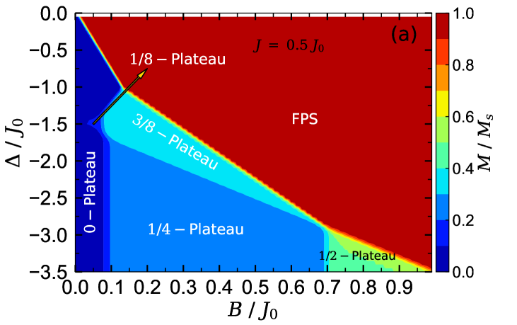
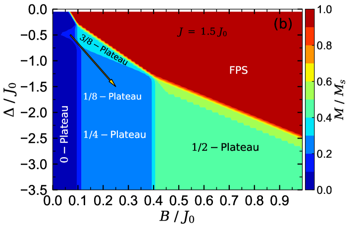
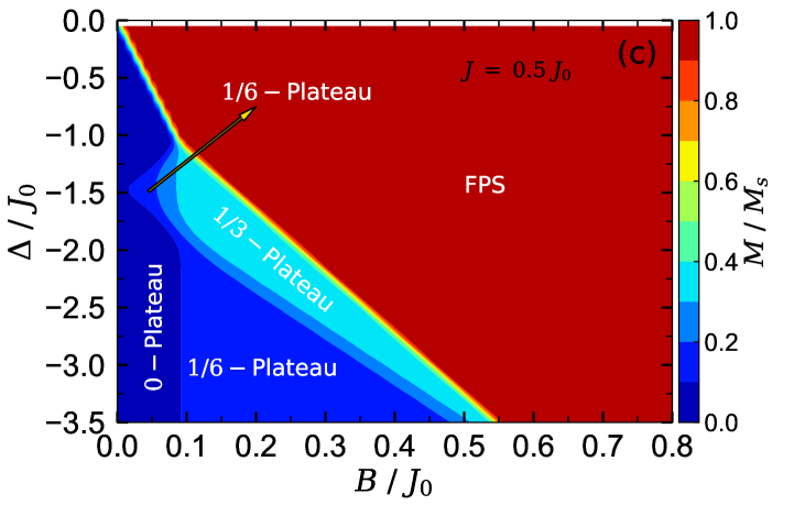
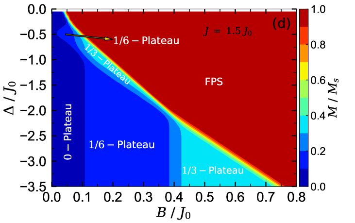
Figure 2: The ground-state magnetic phase diagram of the model in the ($B/J_{0}-\Delta/J_{0}$) plane by considering fixed values: (a) $J=0.5J_{0}$ and $g_{1}=g_{2}=1$; (b) $J=1.5J_{0}$ and $g_{1}=g_{2}=1$; (c) $J=0.5J_{0}$, $g_{1}=1$ and $g_{2}=2$; (d) $J=1.5J_{0}$, $g_{1}=1$ and $g_{2}=2$.

Let now study the case $g_{1}\neq g_{2}$, considering the ratio $g_{2}/g_{1}$ being an integer. For $g_{1}=1$ and $g_{2}=2$, as in Figs. 2(c) and 2(d), the model has ground-states with completely different magnetization intermediate plateaux at zero, one-sixth and one-third normalized with respect to its saturation value.

Fig. 3 illustrates the magnetic field dependences of the magnetization per block in the unit of its saturation value for various fixed values of the exchange anisotropy parameter $\Delta/J_{0}$. Panel 3(a) demonstrates the magnetization per block against the magnetic field at low temperature ($T=0.02J_{0}$) and fixed value of the isotropic coupling constant $J=0.5J_{0}$ and $g_{1}=g_{2}=1$, where several values of the anisotropy $\Delta/J_{0}$ have been considered. On the other hand, panel 3(b) displays this quantity versus the magnetic field at a larger coupling constant, $J=1.5J_{0}$, for the same set of other parameters of the panel 3 (a). As mentioned before, the magnetization curve shows intermediate plateaux at zero, one-eighth, one-fourth, three-eighth and one-half of saturation magnetization for anisotropy range $\Delta/J_{0}<0$. It is shown in these figures the magnetization jumps accompanied with the first-order ground-state phase transition between different magnetization plateaux. Critical magnetic fields at which magnetization jumps occur are observable as well. These points strongly depend on both parameters $J/J_{0}$ and $\Delta/J_{0}$.

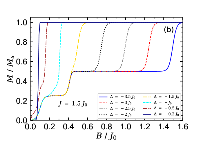
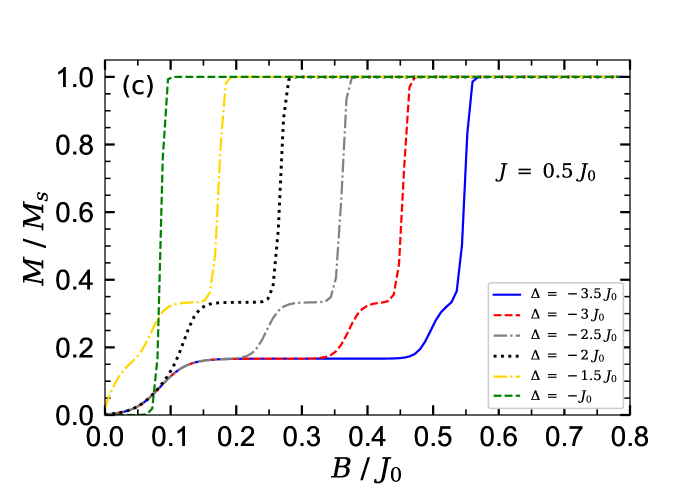
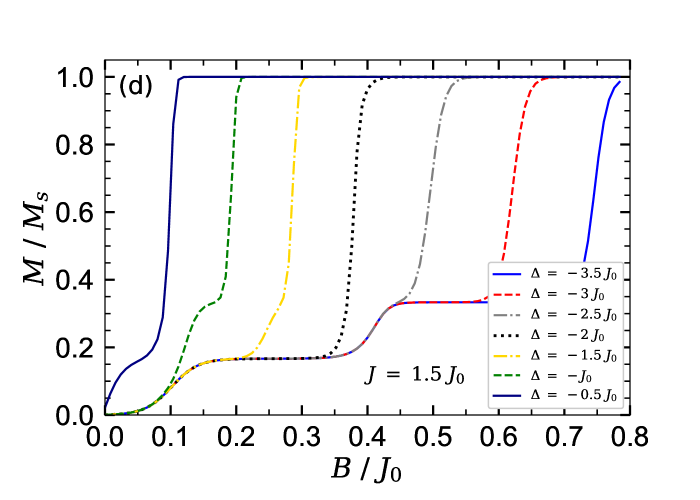
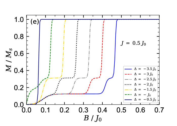
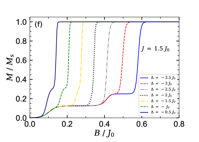
Figure 3: (a) Magnetization in units of the saturation value $M/M_{s}$ as a function of external magnetic field $B/J_{0}$ at temperature $T=0.02J_{0}$ for $J=0.5J_{0}$, $g_{1}=g_{2}=1$ and several exchange anisotropy ratios $\Delta/J_{0}$. (b) $J=1.5J_{0}$, where other parameters are taken as in panel (a). Magnetization for the cases (c) $J=0.5J_{0}$, $g_{1}=1$, $g_{2}=2$; (d) $J=1.5J_{0}$, $g_{1}=1$, $g_{2}=2$; (e) $J=0.5J_{0}$, $g_{1}=1$, $g_{2}=3$; and (f) $J=1.5J_{0}$, $g_{1}=1$, $g_{2}=3$.

It is evident from Fig. 3(b) that by tuning $J/J_{0}$ the magnetization jump occurs at different critical magnetic fields. From the discontinuous ground-state phase transition perspective, when the coupling constant $J/J_{0}$ increases, the transition from the state with magnetization $M/M_{s}=1/4$ to that of with $M/M_{s}=1/2$ occurs at lower magnetic field, while the transition from ground-state with the related magnetization $M/M_{s}=1/2$ to the FPS occurs at stronger magnetic fields compared to the case $J=0.5J_{0}$.

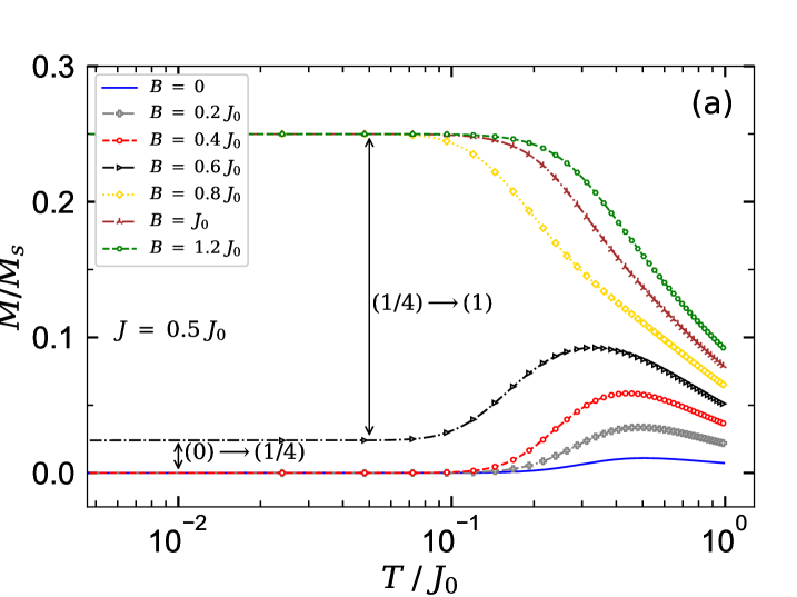
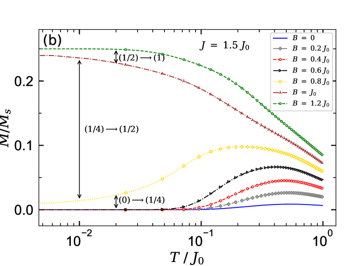
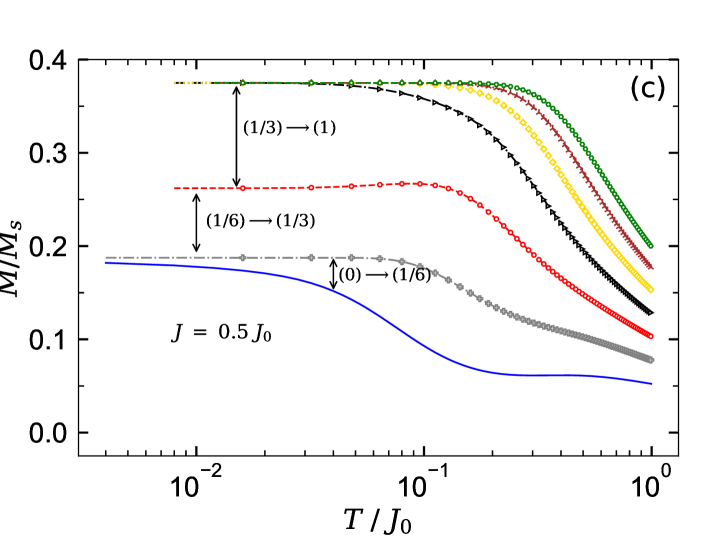
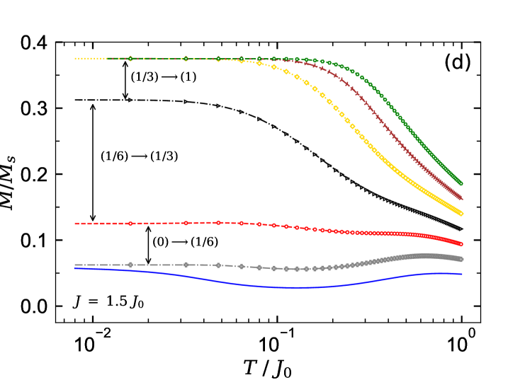
Figure 4: Temperature dependence of the magnetization $M/M_{s}$ for several selected magnetic fields and fixed $\Delta=-1.5J_{0}$, assuming (a) $J=0.5J_{0}$ and $g_{1}=g_{2}=1$; (b) $J=1.5J_{0}$ and $g_{1}=g_{2}=1$; (c) $J=0.5J_{0}$, $g_{1}=1$ and $g_{2}=2$; and (d) $J=1.5J_{0}$, $g_{1}=1$ and $g_{2}=2$.

Again assuming different g-factors $g_{1}=1$ and $g_{2}=2$, we observe significant changes in the magnetization curve of the model. For instance, as shown in Fig. 3(c), when fixed values $J=0.5J_{0}$, $g_{1}=1$ and $g_{2}=2$ are considered, intermediate plateaux at zero, one-sixth and one-third of saturation magnetization appear in the magnetization curve. By increasing the coupling constant $J/J_{0}$, see Fig. 3(d), the width of one-sixth plateau decreases, while the one-third plateau gets wider so that the magnetization jump between these plateaux occurs at a lower magnetic field.

Fig. 4(a) displays the temperature dependence of the magnetization for several fixed values of the magnetic field for $J=0.5J_{0}$, $g_{1}=g_{2}=1$ and at a fixed $\Delta=-1.5J_{0}$. The main effect of the temperature on the magnetization is to aggregate the magnetization curves which are strictly discontinuous at finite low temperatures. The magnetization gaps in this figure denote the magnetization jump from one plateau to another. Numbers in parentheses indicate the magnetization plateaux normalized with respect to its saturation value. For example, $(0)\longrightarrow(1/4)$ means jumping from the zero plateau to the one-fourth plateau in the magnetization curve. The magnetization gaps corresponding to the jumps from one-fourth to one-half and from one-half to the saturation magnetization are quite evident in Fig. 4(b).

The results illustrated in Figs. 4(c) and 4(d) highlight that the magnetization behavior against temperature for the case $g_{1}=1$ and $g_{2}=2$ is substantially different from the case $g_{1}=g_{2}=1$.

For the more general case $g_{1}=1$ and $g_{2}=ng_{1}$ with $n=1,\;2,\;3,\;\cdots$, each magnetization plateau can be successfully identified in terms of the considered Landé g-factors. By inspection we find

$$\begin{array}[]{lcl}\begin{cases}\text{$g_{1}=1$}\\ \text{$g_{2}=1$}\\ \end{cases}\Rightarrow M/M_{s}=\begin{cases}\text{$\frac{2}{8}$}\\ \text{$\frac{3}{8}$}\\ \text{$\frac{4}{8}$}\\ \text{$\frac{1}{8}$}\end{cases}\equiv\begin{cases}\text{$\dfrac{\frac{\alpha}{2}g_{1}}{\alpha(g_{1}+g_{2})}$}\\ \text{$\dfrac{\frac{\alpha}{2}g_{1}+g_{2}}{\alpha(g_{1}+g_{2})}$}\\ \text{$\dfrac{2(g_{1}+g_{2})}{\alpha(g_{1}+g_{2})}$}\\ \text{$\dfrac{g_{2}}{\alpha(g_{1}+g_{2})}$}\end{cases},\\ \\ \begin{cases}\text{$g_{1}=1$}\\ \text{$g_{2}=2$}\\ \end{cases}\Rightarrow M/M_{s}=\begin{cases}\text{$\frac{1}{6}$}\\ \text{$\frac{2}{6}$}\\ \end{cases}\equiv\begin{cases}\text{$\dfrac{\frac{\alpha}{2}g_{1}}{\alpha(g_{1}+g_{2})}$}\\ \text{$\dfrac{g_{2}}{\alpha(g_{1}+g_{2})}$}\\ \end{cases},\\ \\ \begin{cases}\text{$g_{1}=1$}\\ \text{$g_{2}=3$}\\ \end{cases}\Rightarrow M/M_{s}=\begin{cases}\text{$\frac{1}{8}$}\\ \text{$\frac{5}{16}$}\\ \text{$\frac{3}{16}$}\end{cases}\equiv\begin{cases}\text{$\dfrac{\frac{\alpha}{2}g_{1}}{\alpha(g_{1}+g_{2})}$}\\ \text{$\dfrac{\frac{\alpha}{2}g_{1}+g_{2}}{\alpha(g_{1}+g_{2})}$}\\ \text{$\dfrac{g_{2}}{\alpha(g_{1}+g_{2})}$}\end{cases};\end{array}$$ (11)

similar expressions could be carried out by increasing $n$. In Eqs. (11) it is

$$\alpha=2+[1+(-1)^{g_{1}+g_{2}}].$$

Figs. 3(e) and 3(f) illustrate the validity of the results (11). E.g., in Fig. 3(e) it is shown the magnetization per saturation against the magnetic field for the situation $g_{1}=1$ and $g_{2}=3$, where $J=0.5J_{0}$. It is clear that there are magnetization intermediate plateuax at $M/M_{s}=1/8$, $M/M_{s}=5/16$ and $M/M_{s}=3/16$, in agreement with the corresponding relationships noted in Eq. (11).

III.2 Entropy and internal energy

The magnetic field variations of the magnetization near the ground-state phase boundaries may manifest themselves also in unusual behaviors of basic thermodynamic quantities, so we hereby explore in the following the temperature dependence of the entropy and internal energy for different magnetic fields.

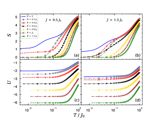
Figure 5: (a) Entropy of the spin-1/2 Ising-Heisenberg Cairo pentagonal model as a function of the temperature for several fixed values of the magnetic field $B/J_{0}$ at fixed coupling constant $J=0.5J_{0}$. (b) The same as in panel (a), but with $J=1.5J_{0}$. Panels (c) and (d) illustrate the temperature dependence of the internal energy for the same selected magnetic fields and fixed values of other parameters as in panels (a) and (b), respectively. In all panels it is assumed fixed anisotropy $\Delta=-1.5J_{0}$ and $g_{1}=g_{2}=1$.

Figs. 5(a) and 5(b) show thermal variations of the entropy at different magnetic fields on a logarithmic scale for $\Delta=-1.5J_{0}$, assuming $J=0.5J_{0}$ and $J=1.5J_{0}$, respectively. As argued in Ref. Rodrigues in the absence of the magnetic field, the residual entropy at $J=0.5J_{0}$ is given by $S\longrightarrow\mathrm{ln}(3)$ when $T\longrightarrow 0$. By applying a weak magnetic field ($0<B\lesssim 0.2J_{0}$) the residual entropy at $J=0.5J_{0}$ decreases such that $S<\mathrm{ln}(3)$ when $T\longrightarrow 0$. When the magnetic field becomes larger than $\approx 0.2J_{0}$, the system is highly influenced by magnetization one-fourth and one-half plateaux with residual entropy $S\longrightarrow 0$ when $T\longrightarrow 0$. For the case $J=1.5J_{0}$, even if a weak magnetic field is applied, the system is dominated by ground-state phases associated to the one-fourth and one-half plateaux with residual entropy $S\longrightarrow 0$ when $T\longrightarrow 0$. Figs. 5 (c) and 5 (d) display the internal energy $U=f+TS$, for the same set of parameters considered in Figs. 5 (a) and 5 (b), respectively. Obviously, by applying an external magnetic field the internal energy remarkably decreases at low temperatures.

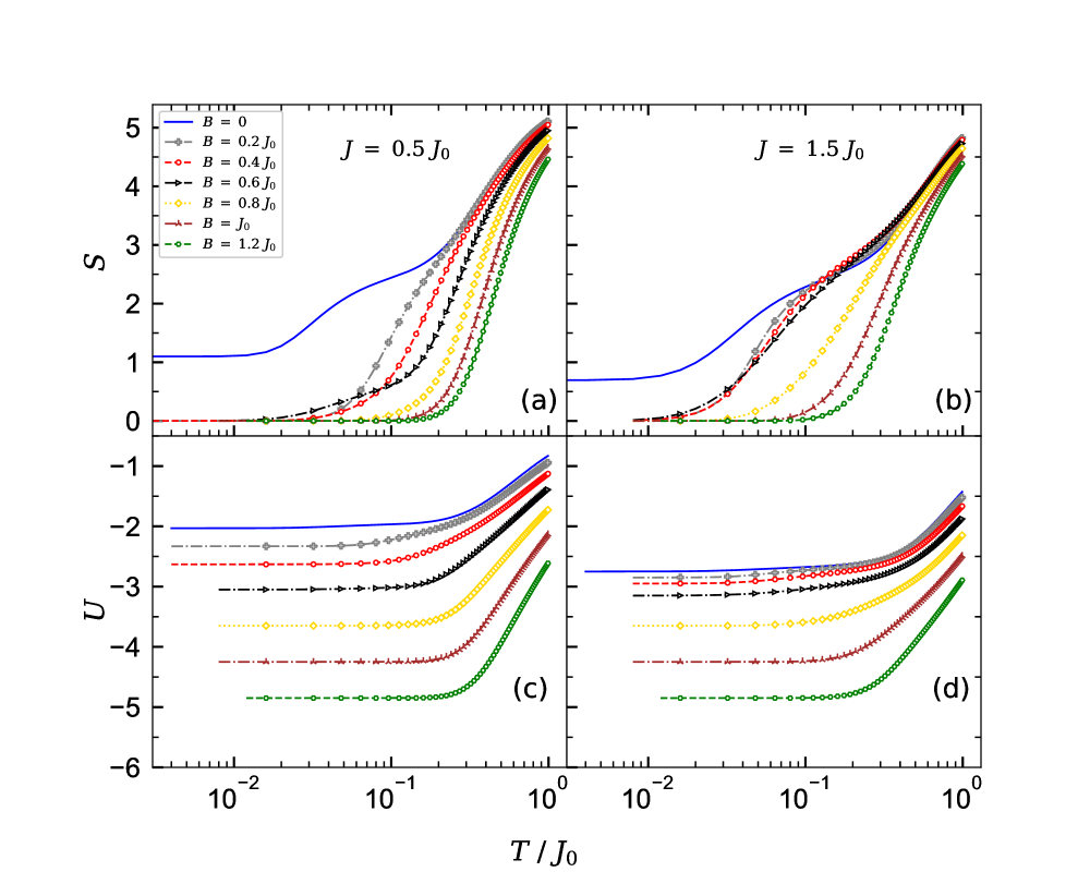
Figure 6: (a) Entropy of the spin-1/2 Ising-Heisenberg Cairo pentagonal model as a function of the the ratio $T/J_{0}$ for several fixed magnetic fields and $J=0.5J_{0}$. (b) The same as in panel (a), but with $J=1.5J_{0}$. In (c) and (d) we plot the temperature dependence of the internal energy of the model for the same selected magnetic fields and the same fixed values of other parameters as in panels (a) and (b), respectively. In all panels ii is $\Delta=-1.5J_{0}$, and $g_{1}=1$ and $g_{2}=2$.

Let consider now $g_{1}=1$ and $g_{2}=2$. Figs. 6(a) and 6(b) show the entropy as a function of the temperature on the logarithmic scale for the case when these different g-factors are considered. By inspecting Fig. 6(a) and comparing it with Fig. 5(a), one can observe a non-trivial difference in the entropy behavior versus temperature when an external magnetic field is applied. For more clarity, if we focus on the three selected magnetic fields $B=\{0.2J_{0},\;0.4J_{0},\;0.6J_{0}\}$ we realize that, independent of the ratio $J/J_{0}$, the entropy behaves in a remarkably different way from the case $g_{1}=g_{2}=1$. As depicted in Figs. 6(c) and 6(d), the internal energy has been increased at low temperatures.

III.3 Specific heat

Let us now examine the effects of exchange coupling $J/J_{0}$ and the magnetic field $B/J_{0}$ on the temperature dependence of the specific heat for anisotropy $\Delta=-1.5J_{0}$. We display in Fig. 7(a) the specific heat of the model under consideration as a function of the temperature for several fixed values of the magnetic field by supposing $J=0.5J_{0}$ and $g_{1}=g_{2}=1$. The blue solid line marked with hexagons represents the specific heat curve for $J=0.5J_{0}$ and $\Delta=-1.5J_{0}$ when $B=0$. In Fig. 7 (a) one can see that the specific heat exhibits a double-peak when $B=0$. When the magnetic field increases, two maxima of the double-peak gradually merge together and make a single peak at higher temperature, see for instance the red dashed line marked with cycles corresponding to $B=0.2J_{0}$. With a further increase of the magnetic field ($B\gtrsim 0.2J_{0}$), an anomalous Schottky type maximum arises at higher temperatures (green dashed line marked with hexagons). Comparison between Figs. 7 (a) and 3 (a) shows that the existence of the double-peak in the specific heat curve denotes the magnetization zero plateau in magnetization curve. Therefore, one can conclude that the spin-1/2 Ising-Heisenberg Cairo pentagonal model is in the AFM state when a double-peak is observed in the specific heat curve. The appearence of a single Schottky-peak nearby the critical magnetic field $B\approx 0.3J_{0}$ (when $M/M_{s}=1$) indicates that the system is in the FPS. Remarkably, a small change in the height of the first peak at low temperature, $T\approx 0.1J_{0}$, is accompanied with the magnetization jump from the zero plateau to the one-fourth plateau, see the evolution of specific heat from the red dashed line marked with cycles to the gold dotted line marked with diamonds illustrated in Fig. 7(a). In fact, the height of the first peak gradually increases as the magnetic field increases, then slightly decreases for the magnetic field interval $0.2J_{0}\lesssim B\lesssim 0.3J_{0}$.

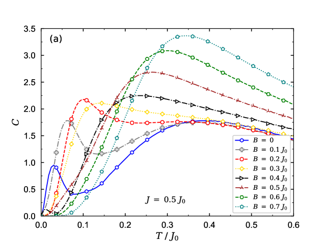
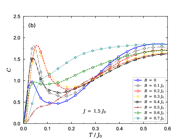
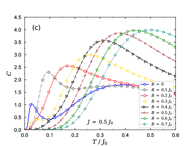
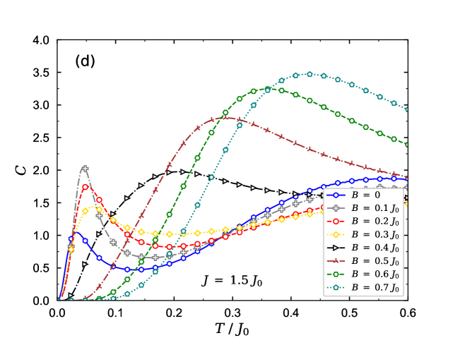
Figure 7: The specific heat of the spin-1/2 Ising-Heisenberg Cairo pentagonal model as a function of the temperature for several values of the magnetic field $B/J_{0}$: (a)$J=0.5J_{0}$, $\Delta=-1.5J_{0}$ and $g_{1}=g_{2}=1$; (b) $J=1.5J_{0}$, $\Delta=-1.5J_{0}$ and $g_{1}=g_{2}=1$; (c) $J=0.5J_{0}$, $\Delta=-1.5J_{0}$, $g_{1}=1$ and $g_{2}=2$; and (d) $J=1.5J_{0}$, $\Delta=-1.5J_{0}$, $g_{1}=1$ and $g_{2}=2$.

To gain further insight into the effects of the coupling constant $J/J_{0}$ on the specific heat, let us also examine the specific heat behavior of the spin-1/2 Ising-Heisenberg Cairo pentagonal model for different values of $J/J_{0}$, which can be of particularly interest especially when the model is in the presence of a tunable magnetic field. We have depicted in Fig. 7(b) the typical dependences of the specific heat on the temperature or several magnetic fields, assuming $J=1.5J_{0}$, $\Delta=-1.5J_{0}$ and $g_{1}=g_{2}=1$. The interesting point from this figure is that the specific heat does not show the single Schottky-peak for range $B\lesssim 0.7J_{0}$. The particular double-peak temperature dependence is observed whose peaks discontinuously change in height upon increasing the magnetic field. The rise and fall of the height of first peak appeared at lower temperatures is accompanied with the presence of magnetization plateaux.

Finally, the specific heat has a Schottky-type maximum at higher temperature and for large magnetic fields $B\gtrsim 0.7J_{0}$, revealing the model is in a FPS. Another interesting thing is that the Schottky-type maximum appears for magnetic fields quite larger than the case $J=0.5J_{0}$. This phenomenon indicates the existence of a magnetization intermediate plateau at one-half of saturation magnetization for the case $J=1.5J_{0}$. Consequently, when the coupling constant $J/J_{0}$ take larger values, the single Schottky peak occurs for magnetic fields larger than the ones for $J=0.5J_{0}$. This scenario is in agreement with the width alterations of intermediate $1/2-$plateau, as shown in Fig. 2(b).

For completeness, Fig. 7(c) shows the specific heat versus temperature for a number of selected magnetic fields, assuming $\Delta=-1.5J_{0}$, $J=0.5J_{0}$, $g_{1}=1$ and $g_{2}=2$. It is clear that the Schottky maximum appears at lower magnetic field and higher temperature intervals. By increasing $J/J_{0}$, as reported in Fig. 7(d), the distance between the peaks of the double peak structure increases and the single maximum arises at considerably lower magnetic fields ($B\gtrsim 0.4J_{0}$) with respect to the case when $g_{1}=g_{2}=1$.

IV Conclusions

In summary, we have investigated the thermodynamic and magnetic properties of the spin-1/2 Ising-Heisenberg Cairo pentagonal model in the presence of an external tunable magnetic field. The magnetization process, entropy, internal energy and the specific heat of this model have been studied by means of the solution obtained within the transfer-matrix formalism. The possibility of having different Landé g-factors was considered.

We showed that the magnetization exhbits intermediate plateaux at zero, one-fourth and one-half of the saturation magnetization when the same Landé g-factors are assumed for the nodal Ising spins and dimer spins. The width of these plateaux depends on the both the isotropic and anisotropic Heisenberg exchange couplings considered for the dimers. By decreasing the anisotropic exchange coupling, the magnetization intermediate one-fourth and one-half plateaux gradually appear. Increasing the isotropic coupling constant results in widening the width of one-half plateau and decreasing the width of one-fourth one. The magnetic field variations considerably affect the entropy and the internal energy when the temperature goes to zero. When different g-factors are considered, different intermediate plateaux are obtained. We also observed a substantial change in entropy behavior and internal energy of the model. We focused on the case in which the ratio between the Landé g-factors is an integer, and it would be interesting to consider in the future both the more general case in which the ratio is a rational number and the situation in which the g-factors are incommensurable.

It has been already shown that in the absence of magnetic field the specific heat curve of the model manifests a visible double-peak structure Rodrigues . Here, we have shown that turning on and varying the magnetic field and the isotropic coupling constant can remarkably modify the shape and the temperature position of this double-peak. One of he most interesting result we found is provided by the magnetic field dependence of the specific heat, for which the rises and falls of the first peak are well in agreement with the entity of magnetization plateaux. We concluded that one can recognize the lowest-energy eigenstate of the model by investigating the evolution of first peak of the double-peak. With a further increase of the magnetic field, the first peak gradually disappears and a single Schottky peak is created at higher temperatures. This single Schottky peak indicates that the model is in the fully polarized phase. As a result, varying the exchange interactions between dimer spins and selecting different Landé g-factors have notable effects on the specific heat behavior versus temperature.

Finally, we mention that it would be interesting to consider more general configurations in which spin-1/2 Ising-Heisenberg Cairo pentagonal chains are connected, starting from the case in which they are merged as a $Y$-junction wiht a variable leg, a geometry which has been considered for XX and Ising quantum spin models Crampe ; Tsvelik ; Giuliano .

References

- (1) G. Vidal, J. I. Latorre, E. Rico and A. Kitaev, Phys. Rev. Lett. 90, 227902 (2003).
- (2) B. Gu and G. Su, Phys. Rev. B 75, 174437 (2007).
- (3) R. Dillenschneider, Phys. Rev. B 78, 224413 (2008).
- (4) N. B. Ivanov, J. Richter and J. Schulenburg, Phys. Rev. B 79, 104412 (2009).
- (5) T. Werlang, C. Trippe, G. A. P. Ribeiro and G. Rigolin, Phys. Rev. Lett. 105, 095702 (2010).
- (6) S. Sachdev, Quantum Phase Transitions (Cambridge University Press, Cambridge, 2011).
- (7) O. Rojas, M. Rojas, N. S. Ananikian and S. M. de Souza, Phys. Rev. A 86, 042330 (2012).
- (8) J. Torrico, M. Rojas, S. M. de Souza, O. Rojas and N. S. Ananikian, Europhys. Lett. 108, 50007 (2014).
- (9) J. Strečka, R. C. Alécio, M. Lyra and O. Rojas, J. Magn. Magn. Mater. 409, 124 (2016).
- (10) A. Koga, S. Kumada, N. Kawakami and T. Fukui, J. Phys. Soc. Jpn. 67, 622 (1998).
- (11) K. Okamoto, N. Okazaki and T. Sakai, J. Phys. Soc. Jpn. 71, 196 (2002).
- (12) M. Müller, T. Vekua and H.-J. Mikeska, Phys. Rev. B 66, 134423 (2002).
- (13) T. Vuletić, B. Korin-Hamzić, T. Ivek, S. Tomić, B. Gorshunov, M. Dressel and J. Akimitsu, Phys. Rep. 428, 169 (2006).
- (14) S. Notbohm, Spin Dynamics of Quantum Spin-Ladders and Chains, PhD thesis (University of St. Andrews, 2007).
- (15) S. Chen, H. Büttner and J. Voit, Phys. Rev. B 67, 054412 (2003).
- (16) S. A. Blundell and M. D. Núñez-Regueiro, Eur. Phys. J. B 31, 453 (2003).
- (17) O. Le Bacq, A. Pasturel, C. Lacroix and M. D. Núñez-Regueiro, Phys. Rev. B 71, 014432 (2005).
- (18) H. Arian Zad and N. Ananikian, J. Phys. Condens. Matt. 29, 455402 (2017).
- (19) X. Y. Feng, G. M. Zhang and T. Xiang, Phys. Rev. Lett. 98, 087204 (2007).
- (20) G. Ghelli, G. Magnifico, C. Degli E. Boschi and E. Ercolessi, Phys. Rev. B 101, 085124 (2020).
- (21) A. M. Läuchli, J. Sudan and R. Moessner, Phys. Rev. B 100, 155142 (2019).
- (22) J. Schnack, J.Schulenburg and J. Richter, Phys. Rev. B 98, 094423 (2018).
- (23) S. Yan, D. A. Huse and S. R. White, Science 332, 1173 (2011).
- (24) F. Kolley, S. Depenbrock, I. P. McCulloch, U. Schollwöck and V. Alba, Phys. Rev. B 91, 104418 (2015).
- (25) M. Drillon, M. Belaiche, P. Legoll, J. Aride, A. Boukhari and A. Moqine, J. Magn. Magn. Mater. 128, 83 (1993).
- (26) K. Okamoto, T. Tonegawa, M. Kaburagi and M. Kaburagi, J. Phys.: Condens. Matter. 11, 10485 (1999).
- (27) K. Okamoto, T. Tonegawa and M. Kaburagi, J. Phys.: Condens. Matter. 15, 5979 (2003).
- (28) D. Uematsu and M. Sato, J. Phys. Soc. Jpn. 76, 084712 (2007).
- (29) H. Kikuchi, Y. Fujii, M. Chiba, S. Mitsudo, T. Idehara and T. Kuwai, J. Magn. Magn. Mater. 272, 900 (2004).
- (30) H. Kikuchi, Y. Fujii, M. Chiba, S. Mitsudo, T. Idehara, T. Tonegawa, K. Okamoto, T. Sakai, T. Kuwai and H. Ohta, Phys. Rev. Lett. 94, 227201 (2005).
- (31) A. Baniodeh, N. Magnani, Y. Lan, G. Buth, C. E. Anson, J. Richter, M. Affronte, J. Schnack and A. K. Powell, npj Quant. Mater 3, 10 (2018).
- (32) M. Rojas, O. Rojas and S. M. de Souza, Phys. Rev. E 86, 051116 (2012).
- (33) I. Rousochatzakis, A. M. Läuchli, and R. Moessner, Phys. Rev. B 85, 104415 (2012).
- (34) F. C. Rodrigues, S. M. de Souza and O. Rojas, Annals of Phys. 379, 1 (2017).
- (35) S. N. Saadatmand, B. J. Powell and I. P. McCulloch, Phys. Rev. B 91, 245119 (2015).
- (36) J. S. Valverde, O. Rojas and S. M. de Souza, J. Phys.: Condens. Matt. 20, 345208 (2008).
- (37) N. S. Ananikian, L. N. Ananikyan, L. A. Chakhmakhchyan and O. Rojas, J. Phys.: Condens. Matt. 24, 256001 (2012).
- (38) V. S. Abgaryan, N. S. Ananikian, L. N. Ananikyan and V. Hovhannisyan, Solid State Comm. 203, 5 (2015); V. S. Abgaryan, N. S. Ananikian, L. N. Ananikyan and V. Hovhannisyan, Solid State Comm. 224, 15 (2015).
- (39) O. Rojas, M. Rojas, S. M. de Souza, J. Torrico, J. Strečka and M. L. Lyra, Physica A 486, 367 (2017).
- (40) H. Arian Zad and N. Ananikian, J. Phys. Condens. Matt. 30, 165403 (2018).
- (41) A. Campa, G. Gori, V. Hovhannisyan, S. Ruffo and A. Trombettoni, J. Phys. A 52, 344002 (2019).
- (42) V. M. L. D. Prasad Goli, S. Sahoo, S. Ramasesha and D. Sen, J. Phys.: Condens. Matt. 25, 125603 (2013).
- (43) S. Sahoo, V. M. L. D. Prasad Goli, D.Sen and S. Ramasesha, J. Phys.: Condens. Matt. 26, 276002 (2014).
- (44) G. Giri, D. Dey, M. Kumar, S. Ramasesha and Z. G. Soos, Phys. Rev. B 95, 224408 (2017).
- (45) V. Hovhannisyan, J. Strečka and N. Ananikian, J. Phys.: Condens. Matt. 28, 085401 (2016).
- (46) K. Hida, J. Phys. Soc. Jpn. 63, 2514 (1994).
- (47) T. Verkholyak, J. Strečka, M. Jaščur and J. Richter, Eur. Phys. J. B 80, 433 (2011).
- (48) D. C. Cabra, A. Honecker and P. Pujol, Phys. Rev. Lett. 79, 5126 (1997).
- (49) K. Karľová, J. Strečka and T. Madaras, Physica B 488, 49 (2016).
- (50) G. Misguich and B. Bernu, Phys. Rev. B 71, 014417 (2005).
- (51) G. Misguich and P. Sindzingre, Eur. Phys. J. B 59, 305 (2007).
- (52) J. S. Helton, K. Matan, M. P. Shores, E. A. Nytko, B. M. Bartlett, Y. Yoshida, Y. Takano, A. Suslov, Y. Qiu, J.-H. Chung, D. G. Nocera and Y. S. Lee, Phys. Rev. Lett. 98, 107204 (2007).
- (53) V. Ohanyan, O. Rojas, J. J. Strečka and S. Bellucci, Phys. Rev. B 92, 214423 (2015).
-
(54)
T. Krokhmalskii, T. Verkholyak, O. Baran, V. Ohanyan and O. Derzhko,
arXiv:2001.04159 - (55) J. Yeomans, Statistical mechanics of phase transitions (Clarendon, Oxford, 1992).
- (56) N. Crampé and A. Trombettoni, Nucl. Phys. B 871, 526 (2013).
- (57) A. M. Tsvelik, Phys. Rev. Lett. 110, 147202 (2013).
- (58) D. Giuliano, P. Sodano, A. Tagliacozzo and A. Trombettoni, Nucl. Phys. B 909, 135 (2016).