L2P: Learning to Place for
Estimating Heavy-Tailed Distributed Outcomes

Abstract

Many real-world prediction tasks have outcome variables that have characteristic heavy-tail distributions. Examples include copies of books sold, auction prices of art pieces, demand for commodities in warehouses, etc. By learning heavy-tailed distributions, “big and rare” instances (e.g., the best-sellers) will have accurate predictions. Most existing approaches are not dedicated to learning heavy-tailed distribution; thus, they heavily under-predict such instances. To tackle this problem, we introduce Learning to Place (L2P), which exploits the pairwise relationships between instances for learning. In its training phase, L2P learns a pairwise preference classifier: is instance A $>$ instance B? In its placing phase, L2P obtains a prediction by placing the new instance among the known instances. Based on its placement, the new instance is then assigned a value for its outcome variable. Experiments on real data show that L2P outperforms competing approaches in terms of accuracy and ability to reproduce heavy-tailed outcome distribution. In addition, L2P provides an interpretable model by placing each predicted instance in relation to its comparable neighbors. Interpretable models are highly desirable when lives and treasure are at stake.

1 Introduction

Heavy-tailed distributions are prevalent in real world data. By heavy-tailed, we mean a variable whose distribution has a heavier tail than the exponential distribution. Many real-world applications involve predicting heavy-tailed distributed outcomes. For example, publishers want to predict a book’s sales number before its publication in order to decide the advance for the author, effort in advertisement, copies printed, etc [1]. Galleries are interested in an artist’s selling potential to decide whether to represent the artist or not. For inventory planning, warehouses and shops would like to know what number of each item to keep in storage [2]. All of these real-world applications involve heavy-tailed distributed outcomes – book sales, art auction prices, and demands for items.

The challenge for predicting heavy-tailed outcomes lies at the tail of the distributions, i.e., the “big and rare” instances such as best-sellers, high-selling art pieces and items with huge demands. Those instances are usually the ones that attract the most interests and create the most market values. Traditional approaches tend to under-predict the rare instances at the tail of the distribution. The limiting factor for prediction performance is the insufficient amount of training data on the rare instances. Approaches tackling class imbalance problem, such as over-sampling training instances [3], adjusting weights, and adding extra constraints [4, 5, 6, 7] do not properly address the aforementioned problem, since those approaches assume homogeneously distributed groups with proportionally different sizes. In addition, defining distinct groups on a dataset with heavy-tailed outcomes is not trivial since the distribution is continuous. Therefore, predicting the values of heavy-tailed variables is not merely the class imbalance problem; instead it is the problem of learning a heavy-tailed distribution.

We present an approach called Learning to Place (L2P) to estimate heavy-tailed outcomes and define performance measures for heavy-tailed target variables prediction. L2P learns to estimate a heavy-tailed distribution by first learning pairwise preferences between the instances and then placing the new instance within the known instances and assigning an outcome value. Our contributions are as follows:

1. We introduce Learning to Place (L2P) to estimate heavy-tailed outcomes by (i) learning from pairwise relationships between instances and (ii) placing new instances among the training data and predicting outcome values based on those placements.

2. We present appropriate statistical metrics for measuring the performance for learning heavy-tailed distributions.

3. In an exhaustive empirical study on real-world data, we demonstrate that L2P is robust and consistently outperforms various competing approaches across diverse real-world datasets.

4. Through case studies, we demonstrate that L2P not only provides accurate predictions but also is interpretable.

The outline of the paper is as follows. Section 2 presents our proposed method. Section 3 describes our experiments. Section 4 explains how our method produces models that are interpretable. Section 5 contains related work and a discussion of our findings. The paper concludes in Section 6.

2 Proposed Method: Learning to Place (L2P)

L2P takes as input a data matrix where the rows are data instances (e.g., books) and the columns are features that describe each instance (e.g., author, publisher, etc). Each data instance also has a value for the predefined target variable (e.g., copies of book sold). L2P learns to map each instance’s feature vector to the value for its target variable, which is the standard supervised learning setup. However, the challenges that L2P addresses are as follows. First, it learns the heavy-tailed distribution of the target variable; and thus it does not under-predict the “big and rare” instances. Second, it generates an interpretable model for the human end-user (e.g., a publisher).

Figure 1 describes the training and placing phases for L2P. In the training phase, L2P learns a pairwise-relationship classifier, which predicts whether the target variable for an instance A ($I_{A}$) is greater (or less) than another instance B ($I_{B}$). To predict outcomes in the placing phase, the unplaced instance is compared with each training instance using the model learned in the training phase, generating pairwise-relationships between the unplaced instance and the training instances. These pairwise-relationships are then used as “votes” to predict the target outcome of the new instance.

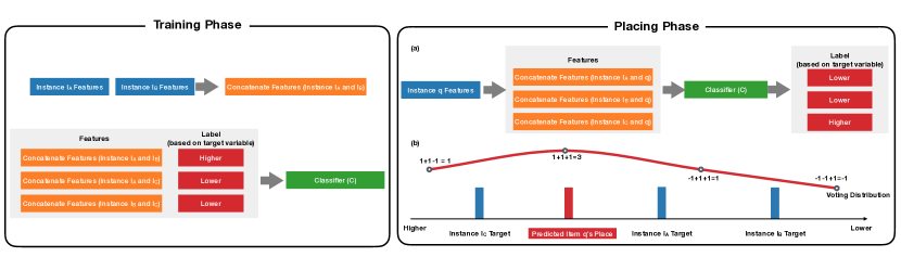
Figure 1: Overview of the L2P Algorithm. In the training phase, L2P learns a classifier $C$ on the pairwise-relationship between each pair of training instances. In the placing phase, L2P applies the classifier $C$ to obtain the pairwise relationships between unplaced instance $q$ and all of the training instances. Then, each instance in the training set contributes to the placement of unplaced instance $q$ by voting on bins to its left or to its right depending on the predicted relation between instances. The mid-value of the bin with the highest vote is assigned as the prediction.

Training Phase. For each pair of instances $i$ and $j$ with feature vector $f_{i}$ and $f_{j}$, L2P concatenates the two feature vectors $X_{ij}=[f_{i},f_{j}]$. If $i$’s target variable is greater than $j$’s, then $y_{ij}=1$; otherwise, $y_{ij}=-1$ (ties are ignored in the training phase). Formally, denoting with $t_{i}$ the target variable for instance $i$ and with $S$ the set of instances in the training set, L2P generates the following training data:

$$X_{ij}=[f_{i},f_{j}],\text{ for each}(i,j)\in S\times S,i\neq j\ ,t_{i}\neq t_{j},$$ (1)

$$y_{ij}=\begin{cases}1,&t_{i}>t_{j}\\ -1,&t_{i}<t_{j}\end{cases}.$$ (2)

Then a classifier $C$ is trained on the training data $X_{ij}$ and labels $y_{ij}$. It is important to note that the trained classifier may produce conflicting results: for example, $I_{A}<I_{B}$ and $I_{B}<I_{C}$ but $I_{C}<I_{A}$. In the Experiments section, we demonstrate the robustness of L2P to such conflicts rooted from the pairwise classification error.

Placing Phase. The placing phase consists of two stages. In Stage I, for each unplaced instance $q$, L2P obtains $X_{iq}=[f_{i},f_{q}],\text{ for each }i\in S$ (recall $S$ is the training set). Then, L2P applies the classifier $C$ on $X_{iq}$ to get the predicted pairwise relationship between the test instance $q$ and all training instances ($\hat{y}_{iq}=C(X_{iq})$). In Stage II, L2P treats each training instance as a “voter”. Training instances (voters) are sorted by their target variables in descending order, dividing the target variable axis into bins. If $\hat{y}_{iq}=1$, bins on the right of $t_{i}$ will obtain an upvote (+1) and bins on the left of $t_{i}$ will obtain a downvote (-1) and vice versa for $\hat{y}_{iq}=-1$. After the voting process, L2P takes the bin with the most “votes” as the predicted bin for test instance $q$, and obtains the prediction $\hat{t}_{q}$ as the midpoint of this bin.

2.1 Theoretical Analysis of Voting Process

L2P’s voting process can be viewed as the maximum likelihood estimation (MLE) of the optimal placement of an instance based on the pairwise relationships. Given the test instance $q$, our goal is to find its optimal bin $m$. For any bin $b$, we have: $P(b|q)\propto P(q|b)\times P(b)$. Since each train instance $i$ contributes to $P(q|b)$, we have $P(q|b)=\frac{1}{Z}\sum_{i\in S_{train}}P_{i}(q|b)$, where $P_{i}(q|b)$ is the conditional probability of test instance $q$ placing in the given bin $b$ based on its pairwise relationship with training instance $i$; and $Z$ is the normalization factor, $Z=\sum_{b}\sum_{i}P_{i}(q|b)$. L2P assigns two probabilities to each pair of training instance $i$ and test instance $q$: $p_{i}^{l}(q)$ and $p_{i}^{r}(q)$, denoting the probability that the test instance $q$ is smaller than (i.e., to the left of) or larger than (i.e., to the right of) training instance $i$ respectively, where $p_{i}^{l}(q)+p_{i}^{r}(q)=1$. Let $R_{b}^{i}\in\{l,r\}$ be the region defined by training instance $i$ for bin $b$, and $|R_{b}^{i}|$ as the number of bins in this region. We know $P_{i}(q|b)=p_{i}^{R_{b}^{i}}(q)/|R_{b}^{i}|$ assuming the test instance is equally probable to fall in each bin in region $R_{m}^{i}$. Therefore, the optimal bin is $m=\text{argmax}_{b}\frac{1}{Z}\sum_{i\in S}(p_{i}^{R_{b}^{i}}(q)/|R_{b}^{i}|)$. We observe that $p_{i}^{R_{b}^{i}}(q)/|R_{b}^{i}|$ is the “votes” the training instance $i$ gives to bin $b$ for test instance $q$, therefore the optimal bin $m$ is the one with the most “votes”.

Input: Training data $S=(F,t)$

Output: Pairwise relationship classifier $C$

 // Feature matrix

$X=[\ ]$;

 // Label vector

$y=[\ ]$;

for $i\leftarrow 1$ to $|S|$ do

       for $j\leftarrow i+1$ to $|S|$ do

             $X$.append([$f_{i}$, $f_{j}$]);

             if $t_{i}>t_{j}$ then

                   $y$.append(1)

                  

             else if $t_{i}<t_{j}$ then

                  $y$.append(-1)

                  

            

       end for

      

end for

C.train($X$, $y$);

return C

Algorithm 1 L2P’s Training Algorithm

Input: Classifier $C$, Training data $S$=($F$, $t$), Unplaced instance $q$ represented by its features $f_{q}$

Output: $t_{q}$ = predicted value for test instance $q$

$B=[\ ]$;

 // Unique target values, highest to lowest

bins = sort(unique($t$));

for $i\leftarrow 1$ to $|\text{bins}|$ do

       B[i] = 0

      

end for

for $i\leftarrow 1$ to $|F|$ do

       $\hat{y}_{iq}=C.predict([f_{i},f_{q}])$

       for $j\leftarrow 1$ to BinEdgeIndex($t_{i}$) - 1 do

             B[j] -= $\hat{y}_{iq}$;

       end for

      for $j\leftarrow$ BinEdgeIndex($t_{i}$) to $|B|$ do

             B[j] += $\hat{y}_{iq}$;

       end for

      

end for

b = GetHighestBin(B);

$t_{q}$ = Mean(bins[b-1], bins[b]);

return $t_{q}$

Algorithm 2 L2P’s Placing Algorithm

L2P can incorporate any method that takes pairwise preferences and learns to place a test instance among the training instances. Specifically, we examined SpringRank [8], FAS-PIVOT [9] and tournament graph related heuristics [10]. We found that the performances of these approaches are quite similar to voting. However, voting – with its linear runtime complexity – is the most computationally efficient method among them.

2.2 Complexity Analysis

Suppose $n$ is the number of instances in the training set. The vanilla training phase for L2P learns pairwise relationships among all pairs in the training set, leading to a $O(n^{2})$ runtime complexity, which is computationally prohibitive for large datasets even though the training phase is an offline process and can be easily parallelized. Thus, we implemented an efficient approach based on the intuition that it is easier for a classifier to learn the pairwise relationship between instances that are far apart than instances that are near each other. Specifically, we define two parameters: $n_{s}$ denoting the number of samples to compare with for each training instance and $k$ denoting the number of instances that are considered near to each training instance. For comparison to each training instance $i$, L2P’s efficient training phase algorithm (1) takes all $k$ near instances of $i$ and (2) uniformly at random samples $n_{s}-k$ non-near instances of $i$. The nearness of two instances is measured by the difference in their target values. Our experiments with the efficient implementation of L2P lead to similar AUC scores for the overall prediction task, but reduced the runtime complexity to $O(n_{s}\times n)$, where $n_{s}<<n$. For instance, $n_{s}$ is 20% of $n$. L2P’s placing phase has a complexity of $O(n)$ for each new (i.e., test) instance.

3 Experiments

In this section, we describe the data used in our experiments, the baseline and competing approaches, experimental methodology, evaluation metrics, and results.

3.1 Datasets

We present results on the following real-world applications:

Book sales: This dataset consists of information about all print nonfiction and fiction books published in the United States in 2015, including features about authors publication history, book summary, authors popularity (details of features see [1]). The goal is to predict the one year book sales using features prior to the book’s publication. We separate nonfiction books and fiction books in the experiment.

Art auctions: This dataset combines information on artists exhibits, auction sales, and primary market quotes. It was previously used to quantify success of artists based on their trajectories of exhibitions [11]. We select 7,764 paintings using vertical logarithmic binning [12]. The features includes previous exhibition records (number of exhibitions, number of exhibitions at different grade), sales records (number of art pieces sold, various statistics of price of previous sold pieces), career length and medium information (full feature list see Supplementary Information Table 1). The prediction task is to predict auction price of an art piece based on artists’ previous sale and exhibition history.

Table 1 provides the summary statistics of these datasets. Specifically, we calculate the kurtosis for each target variable. Kurtosis measures the “tailedness” of the probability distribution. The kurtosis of any univariate normal distribution is 3, and the higher the kurtosis is, the heavier the tails. Complementary cumulative function (CCDF) of real outcomes are shown in Fig. 2.

Name	Instances	Features	Outcome	Kurtosis
Nonfiction	7,641	55	Sales	619.73
Art	7,764	21	Price	597.82
Fiction	2,061	55	Sales	443.08

Table 1: Dataset statistics, sorted by Kurtosis values. Recall that Kurtosis measures the “tailedness” of a real-valued random variable’s probability distribution.

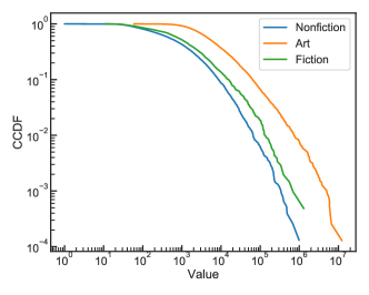
Figure 2: Our target variables, book sales and art auctions, have heavy-tailed distributions.

3.2 Baseline and Competing Approaches

To compare the predictive capabilities of L2P, we experiment with these baseline approaches from the literature.

K-nearest neighbors (kNN). The prediction is obtained through local interpolation of nearest neighbors in the training set.

Kernel regression (KR). We employ Ridge regression with RBF kernels to estimate the non-linear relationship between variables.

Heavy-tailed linear regression (HLR). Hsu and Sabato [13] proposed a heavy-tailed regression model, in which a median-of-means technique is utilized. They proved that for a $d$-dimensional estimator, a random sample of size $\tilde{O}(d\log(1/\delta))$ is sufficient to obtain a constant factor approximation to the optimal loss with probability $1-\delta$. However, this approach is not able to capture non-linear relationships, which exist in our setting.

Neural networks (NN). We use a multi-layer perceptron regressor model. Neural networks sacrifice interpretability for predictive accuracy.

XGBoost (XGB). We use the implementation of gradient boosting optimized on various tasks such as regression and ranking [14].

LambdaMART. We compare with the well-known learning-to-rank algorithm LambdaMART [16]. LambdaMART combines LambdaRank [17] and MART (Multiple Additive Regression Trees) [18]. While MART uses gradient boosted decision trees for prediction tasks, LambdaMART uses gradient boosted decision trees using a cost function derived from LambdaRank for solving a ranking task. Here we choose to optimize LambdaMART based on ranking AUC, which is an appropriate metric for our task. LambdaMART is designed to predict the ranking of a list of items; here we predict the instance by: (1) using LambdaMART to get the ranking of the new instance plus the training instances and (2) predicting the value as the midpoint of actual values of adjacent ranked instances.

Random (RDM). We shuffle actual outcomes at random and assign those random outcomes as predictions.

3.3 Experimental Setup and Evaluation Metrics

We impose standard scaling on all the columns of the data matrix and the target variable. For all competing methods, we first take the logarithm of the entries in the data matrix and the target variable, and then do standard scaling.

For all methods, we employ 5-fold stratified cross-validation to estimate confidence of model performance. For all baseline models, we tune the model parameters to near-optimal performance (parameters listed in Supplementary Information Table 2). For L2P, however, we use the scikit-learn default parameters of random forest classifier, with 100 trees and Gini impurity as split criteria.

Under our problem definition, the model with the best performance will (1) reproduce heavy-tailed outcome distribution and (2) predict instances accurately especially the “big and rare instances”. Traditional regression metrics are not of good fit in this problem setting. For example $R^{2}$ has the assumption of normally distributed error, which is not the case for heavy-tailed distributions; root mean square error (RMSE) will be dominated by the errors on the high end since the values on high-end are extreme. Instead, we use the following metrics that are more appropriate under our circumstances for evaluation:

Quantile-quantile (Q-Q) plot. Q-Q plot can visually present the deviations between true and predicted target variable distributions. A model who can reproduce the outcome distribution should produce curves closer to $y=x$ line. We can also investigate when predicted quantiles deviate from this line.

Kolmogorov-Smirnov statistic (KS) and Earth mover distance (EMD). KS statistic and EMD are two commonly used measure on the distance between two underlying probability distributions. Smaller KS and EMD indicates higher similarity between distributions; and in our analysis, it indicates a better prediction of the underlying distribution.

Receiver operating characteristic (ROC). We calculate true-positive and false-positive rates in order to compute the ROC curve and the area under the ROC curve (a.k.a. AUC score). We adapt AUC calculation to regression setting by calculating the true-positive and false-positive rates at different thresholds (all possible actual values).

True positive rate at threshold. The calculation of true-positive rate (TPR) at threshold follows the recall@k measure used in information retrieval literature. Here, we measure the fraction of instances with true value ($y$) higher than threshold $t$ that also have predicted values ($\hat{y}$) higher than $t$ for calculating TPR. We followed similar approach to compute FPR as in Eq.3.

$$TPR@t=\frac{|\{\hat{y}_{i}\geq t,y_{i}\geq t\}|}{|\{y_{i}\geq t\}|}\text{\ \ \ \ \ \ }FPR@t=\frac{|\{\hat{y}_{i}\geq t,y_{i}<t\}|}{|\{y_{i}<t\}|}$$ (3)

For various thresholds, we compute corresponding TPR and FPR scores to create ROC curve. Similar to traditional ROC curves, a better performing method would have a curve that is simultaneously improving both TPRs and FPRs, leading to a perfect score of AUC = 1. A random model leads to an AUC performance of 0.5 with the corresponding ROC curve being the 45-degree line indicating that TPR and FPR are equal for various thresholds.

It is important to note that each individual measure alone is not sufficient to judge the goodness of a model. KS, EMD and Q-Q plot are measuring the reproducibility of the heavy-tailed distribution, but are not able to measure the prediction accuracy for each instance. Downside of comparing distribution is that the random prediction will end up having the perfect Q-Q plot and KS = 0, EMD = 0. AUC is measuring the accuracy of the prediction, but does not address model’s ability to reproduce the distribution. We aim to harness benefits of different measures to assess quality of our models.

3.4 Experimental Results

Next we detail performance comparisons and robustness analysis.

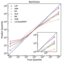
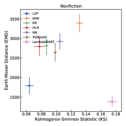
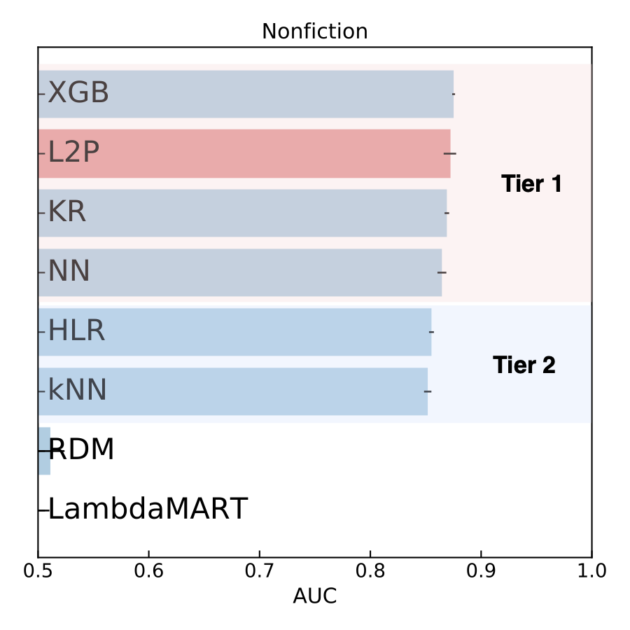
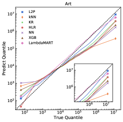
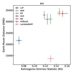
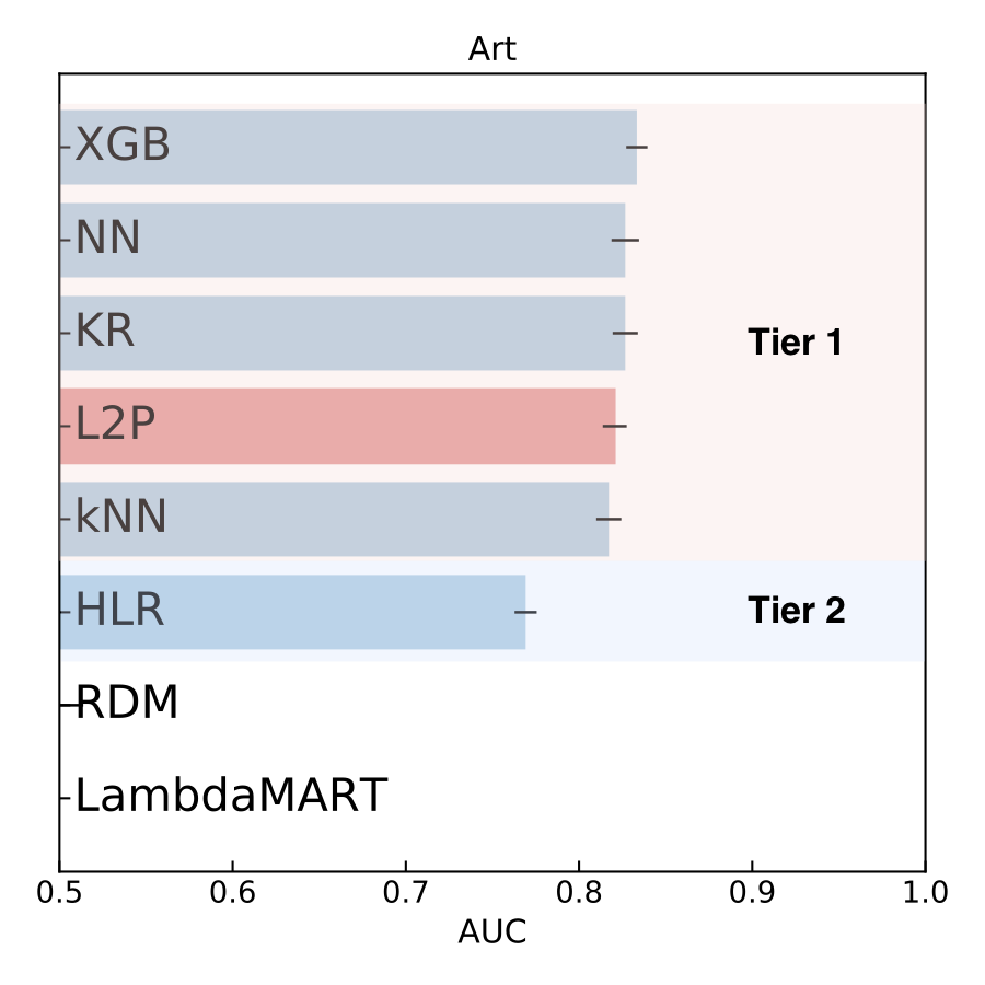
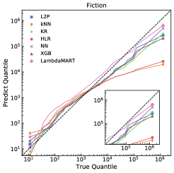
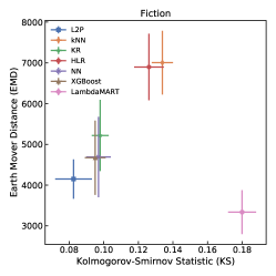
Figure 3: Experimental results. We compare L2P’s performance against 6 other methods (discussed in Section 3.2) across 3 datasets (see Table 1). L2P’s objective is to accurately reproduce the distribution of an outcome variable and accurately predict its value. Q-Q plots (left column) show how predicted and actual quantiles align. L2P reproduces underlying distributions that are accurate at both lower and higher quantiles compared to the other methods. Kolmogorov-Smirnov (KS) statistics and Earth mover distance (EMD) (middle column) measures distance between predicted and actual distributions. The lower the values for KS and EMD, the better. L2P consistently outperforms the other methods. AUC (right column) measures prediction performance. We group methods to tiers based on the mean and standard deviation of the score. L2P achieves top tier performance all datasets. In summary, the only approach that achieves top performance on both reproducing the outcome variable distribution and accurate predictions across the datasets is L2P.

3.4.1 Performance comparison study

We compare the methods using different measurement to showcase that L2P can accurately estimate the heavy-tailed distribution and predict the value of the heavy-tailed variable.

Q-Q plot. In left column in Fig. 3 shows the Q-Q plot of predicted outcomes. In all datasets we see deviation at the high-end (where “big and rare” instances reside). L2P is among the top 3 methods that produce the smallest deviation at the high end for all datasets. LambdaMART is also competitive in producing small deviation, but it produces larger deviations at the low end than L2P.

KS and EMD. The second column of Fig. 3 presents the KS and EMD scores. Outcomes of L2P leads to the smallest KS statistics and second lowest EMD for almost all datasets. LambdaMART shows an advantage on minimizing EMD; however, we will show in AUC score comparison that it is not a preferable method.

AUC. The third column of Fig. 3 shows the AUC score of various methods on different datasets. L2P achieves top tier performance on nonfiction, art and fiction dataset, which all have high kurtosis values. XGB and NN have competitive AUCs to L2P but are bad at reproducing the true distributions as shown previously. We notice that LambdaMART, which has good performance EMD, has very low AUC score, indicating its inability to have accurate prediction on each instance.

We further investigate the possible reasons of the unsatisfying prediction of LambdaMART. Figure 4 shows the ranking results for LambdaMART on the fiction dataset, where we trained and tested on the full dataset. We found that LamdaMART did not correctly rank items that are close to each other. This failure of preserving the rank among training instances is the root cause of why LambdaMART fails to achieve good performance on the new instances prediction.

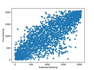
Figure 4: Ranking performance for LambdaMART on the fiction dataset. LambdaMART is trained and tested on the full fiction dataset. We observe that even when trained on the same dataset, LambdaMART’s ranking output is not accurate. While it exhibits general trends around the 45-degree line, the neighborhood ranking is not restored, which is the root cause of why LambdaMART fails to achieve good performance on predictions of new instances.

Takeaway message. With comprehensive consideration of all three evaluations, we can see that L2P is the best method in both reproducing the underlying heavy-tailed distribution and providing accurate predictions.

3.4.2 Robustness analysis

In the placing phase of L2P there are two stages: 1) Stage I: obtaining pairwise relationships between test instance and training instances and 2) Stage II: placing the test instance and obtaining the prediction through voting. Previously we showed that voting itself is a maximum likelihood estimation, therefore the performance of L2P is highly depends on the performance of pairwise relationship learning. Here, we investigate the robustness w.r.t. classification error of pairwise relationships.

To quantify the error tolerance of “voting” and estimation for a new instance, we conduct a set of experiments where we introduce errors on predicting pairwise relationships. We simulate the pairwise relationship error with two mechanisms: (i) random error: constant probability $p=p_{c}$ flips the label for each pair, (ii) distance-dependent error: probability of error is proportional to the true ranking percentile difference between items; here we use the percentile of the ranking because the sizes of the datasets vary. We define the flipping probability as $p_{ij}=e^{-\alpha|r_{i}-r_{j}|}$, assuming it would be easier to learn the pairwise relationship for items that are further away. This is observed in our experiments as well. For example, in nonfiction data, we notice that more than 48% of the pairwise relationship error occurs in item pairs that have a ranking percentile difference smaller than 10. We can control the rate of errors introduced by the two mechanisms by tuning $p_{c}$ or $\alpha$.

In Figure 5, we present the overall performance (AUC) of L2P when various degrees of errors are introduced to the system in the pairwise relationships. First thing to notice is that if the pairwise relationship has no error (see left panel of Figure 5 when classifier accuracy is 1), L2P has an accurate prediction, showing that the performance of the voting stage is only influenced by the quality of the pairwise relationships learned by the model. Moreover, the voting stage can actually compensate errors in pairwise relationships. We observe that error tolerance is significantly high towards random error: performance of L2P is stable until more than 45% of the pairwise relationships are mistaken. For distance-dependent mechanism to simulate errors, we observe robust performance that 30% error in stage I predictions resulting just 20% reduction of the overall performance.

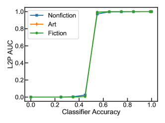
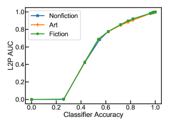
Figure 5: L2P’s Robustness L2P’s AUC scores after random errors (a) or distance-dependent errors (b) are
introduced to L2P’s classifier for pairwise relationships. We observe significantly high tolerance towards random error and gradual degradation in L2P’s overall performance with distance-dependent errors.

4 Model Interpretability

As mentioned earlier, one of the advantages of L2P’s methodology is its interpretability. Let us present the nonfiction book Why not me? by Mindy Kaling as an example. L2P prediction is about 218,000 copies while the actual sales is about 230,000. The key features explaining the success of this particular book are the author’s popularity and the previous sales of author – 6,228,182 pageviews and about 638,000 copies, respectively. However, performance of neural network leads to significant under-prediction of 16,000 sales and it’s not clear why. L2P places Why not me? between Selp-Helf by Miranda Sings and Big Magic by Elizabeth Gilbert. Selp-Helf has the author popularity as 1,390,000 and the author has no prior publishing history, while Big Magic has the author popularity as 1,596,000 and previous sales as 6,954,000. We see that Why not me? has higher author popularity than Big Magic and Selp-Helf, but since it has a lower publishing history than Big Magic, L2P places it between these two books.

We also want to demonstrate an example case where L2P fails to achieve accurate prediction. The nonfiction book The Best Loved Poems of Jacqueline Kennedy Onasis by Caroline Kennedy under Grand Central Publishing, with claimed publication year 2015, is predicted to sell 53,000 copies while the actual sales is 180 copies in the dataset. After an extensive analysis, it turns out that the book was initially published in 2001 and was a New York Times bestseller, which L2P captures its potential and predict high sales. Therefore this incorrect prediction is rooted in data error and our overprediction can be attributed to the initial editions performance as being a best-seller. Neural network predicts 7,150 copies, though closer to the actual sale 180.

5 Related Work and Discussion

Objectives	L2P	kNN	KR	HLR	NN	XGB	LambdaMART
Reproducing heavy-tailness	✓	✗	✗	✗	✓	✗	✓
Accurate predictions	✓	✗	✓	✗	✓	✓	✗
Interpretable model	✓	✓	✗	✓	✗	✗	✓

Table 2: Result summary. We summarize performance of models on different objectives w.r.t. whether they are in the top (✓) or bottom (✗) group. L2P satisfies all the objectives while the competing methods do not.

Learning-to-rank methodologies. Learning-to-rank is the application of machine learning in the construction of ranking models for information retrieval systems. In learning-to-rank, training data consists of lists of items with some partial order specified between items in each list and the ranking model’s purpose is to rank, i.e. produce a permutation of items in new, unseen lists.

Although L2P is designed for predicting heavy-tailed outcomes, which is different from learning-to-rank, methodological contributions show some parallels with the existing ranking algorithms. Cohen et al. [10] proposed a two-phase approach that learns from preference judgments and subsequently combines multiple judgments to learn a ranked list of instances. Similarly, RankSVM [15] is a two-phase approach that translates learning weights for ranking functions into SVM classification. Both of these approaches have complexity $O(n^{2})$, which is computationally expensive.

In experiment practice, we found that learning-to-rank is not satisfying to predict heavy-tailed distributed outcomes. Since the learning-to-rank algorithm cannot guarantee to recover the rankings of the training instances completely, it will end up producing worse prediction on the new instance.

Heavy-tailed regression. Regression problems are known to suffer from under-predicting rare instances [7]. Approaches were proposed to correct fitting models consider prior correction that introduces terms capturing a fraction of rare events in the observations and weighting the data to compensate for differences [4, 6]. Hsu and Sabato [13] proposed a methodology for linear regression with possibly heavy-tailed responses. They split data into multiple pieces, repeat the estimation process several times, and select the estimators based on their performance. They analytically prove that their method can perform reasonably well on heavy-tailed datasets. Quantile regression related approaches are proposed as well. Wang et al. [19] proposed estimating the intermediate conditional quantiles using conventional quantile regression and extrapolating these estimates to capture the behavior at the tail of the distribution. Robust Regression for Asymmetric Tails (RRAT) [20] was proposed to address the problem of asymmetric noise distribution by using conditional quantile estimators. Zhang and Zhou [21] considered linear regression with heavy-tail distributions and showed that using $l1$ loss with truncated minimization can have advantages over $l2$ loss. Like all truncated based approaches, their method requires prior knowledge of distributional properties. However, none of these regression techniques can capture non-linear decision boundaries.

Ordinal Regression. The idea behind L2P methodology is similar to an ordinal regression where each training instance is mapped to an ordinal scale. Previous research has explored ordinal regression using binary classification [22]. The contribution of L2P is that it transforms the prediction of heavy-tailed outcomes to ordinal regression using pairwise-relationship classification followed by an MLE-based voting method. By doing this two-phase approach, L2P is able to reproduce the distribution of the outcome variable and provide accurate predictions for the outcome variable. Combining these two tasks leads consistently to better performance all-around.

Imbalance Learning Data imbalance, as a common issue in machine learning, has been widely studied, especially in classification space. In [23], the problem of imbalance learning is defined as instances have different importance value based on user preference. There are in generally three categories of methods tackling this problem: data pre-processing [3, 24], special-purpose learning methods [25, 26] and prediction post-processing [27, 28]. However, one should notice that learning heavy-tailed distributed attributes is different from imbalance learning. In most imbalance learning, there is a majority group and a minority group, but within group items are mostly homogeneous. However in heavy-tailed distribution, there is no clear cut to define majority/minority group and even if forcing a threshold to form majority/minority group, within each group, the distribution is still heavy-tailed. Additionally, one need to choose a pre-defined relevance function for a lot of methods designed in this space.

Efficient algorithm for pairwise learning. Qian et al. proposed using a two-step hashing framework to retrieve relevant instances and nominate pairs whose ranking is uncertain [29]. Other approaches to efficiently searching for similar pairs and approximately learning pairwise distances are proposed in the literature for information retrieval and image search [30, 31, 32]. L2P can use any robust method that learns pairwise preferences for its pairwise relationships learning.

6 Conclusions

We presented the L2P algorithm, which satisfies three desired objectives consistently: (1) modeling heavy-tail distribution of an outcome variable, (2) accurately making predictions for the heavy-tailed outcome variable, and (3) producing an interpretable ML algorithm as summarized in Table 2. Through learning pairwise relationships following by an MLE-based voting method, L2P preserves the heavy-tailed nature of the outcome variables and avoids under-prediction of rare instances. We observed the following:

1. L2P accurately reproduces the heavy-tailed distribution of the outcome variable and accurately predicts of that variable. Our experimental study, which included 6 competing methods and 3 datasets, demonstrates that L2P consistently outperforms other methods across various performance measures, including accurate estimation of both lower and higher quantiles of the outcome variable distribution, lower Kolmogorov-Smirnov statistic and Earth Mover Distance, and higher AUC.

2. L2P’s performance is robust when errors are introduced in the pairwise-relationship classifier. Under random error setting, L2P can achieve almost perfect performance up to 45% error in pairwise relationship predictions; and under distance-dependent error setting, L2P has an accuracy drop of only 20% with 30% pairwise-relationship error.

3. L2P is an interpretable approach and it provides prediction context. L2P allows one to investigate each prediction by comparing with neighboring instances and their corresponding feature values to obtain more context on the outcome. This is highly important to practitioners such as book publishers, where executives need reasons before making a huge investment.

References

- [1] Xindi Wang, Burcu Yucesoy, Onur Varol, Tina Eliassi-Rad, and Albert-László Barabási. Success in books: predicting book sales before publication. EPJ Data Science, 8(1), 2019.
- [2] Aris A Syntetos, John E Boylan, and Stephen M Disney. Forecasting for inventory planning: a 50-year review. Journal of the Operational Research Society, 60(sup1):S149–S160, 2009.
- [3] Nitesh V Chawla, Kevin W Bowyer, Lawrence O Hall, and W Philip Kegelmeyer. Smote: Synthetic minority over-sampling technique. JAIR, 16, 2002.
- [4] Maher Maalouf, Dirar Homouz, and Theodore B Trafalis. Logistic regression in large rare events and imbalanced data: A performance comparison of prior correction and weighting methods. Computational Intelligence, 34(1), 2018.
- [5] Seyda Ertekin, Jian Huang, Leon Bottou, and Lee Giles. Learning on the border: Active learning in imbalanced data classification. In CIKM, pages 127–136, 2007.
- [6] Max Schubach, Matteo Re, Peter N Robinson, and Giorgio Valentini. Imbalance-aware machine learning for predicting rare and common disease-associated non-coding variants. Scientific Reports, 7(1), 2017.
- [7] Gary King and Langche Zeng. Logistic regression in rare events data. Political Analysis, 9(2), 2001.
- [8] Caterina De Bacco, Daniel B Larremore, and Cristopher Moore. A physical model for efficient ranking in networks. Science Advances, 4(7), 2018.
- [9] Nir Ailon, Moses Charikar, and Alantha Newman. Aggregating inconsistent information: Ranking and clustering. J. ACM, 55(5):23:1–23:27, 2008.
- [10] William W Cohen, Robert E Schapire, and Yoram Singer. Learning to order things. In NIPS, pages 451–457, 1998.
- [11] Samuel P Fraiberger, Roberta Sinatra, Magnus Resch, Christoph Riedl, and Albert-László Barabási. Quantifying reputation and success in art. Science, 362(6416), 2018.
- [12] Keith Henderson, Brian Gallagher, Lei Li, Leman Akoglu, Tina Eliassi-Rad, Hanghang Tong, and Christos Faloutsos. It’s who you know: Graph mining using recursive structural features. In KDD, pages 663–671, 2011.
- [13] Daniel Hsu and Sivan Sabato. Heavy-tailed regression with a generalized median-of-means. In ICML, pages 37–45, 2014.
- [14] Tianqi Chen and Carlos Guestrin. XGBoost: A scalable tree boosting system. In KDD, pages 785–794, 2016.
- [15] Thorsten Joachims. Optimizing search engines using clickthrough data. In KDD, pages 133–142, 2002.
- [16] Christopher JC Burges. From ranknet to lambdarank to lambdamart: An overview. Learning, 11(23-581):81, 2010.
- [17] Christopher J Burges, Robert Ragno, and Quoc V Le. Learning to rank with nonsmooth cost functions. In Advances in neural information processing systems, pages 193–200, 2007.
- [18] Jerome H Friedman. Greedy function approximation: A gradient boosting machine. Annals of Statistics, 29(5):1189–1232, 2001.
- [19] Huixia Judy Wang, Deyuan Li, and Xuming He. Estimation of high conditional quantiles for heavy-tailed distributions. JASA, 107(500):1453–1464, 2012.
- [20] Ichiro Takeuchi, Yoshua Bengio, and Takafumi Kanamori. Robust regression with asymmetric heavy-tail noise distributions. Neural Computation, 14(10):2469–2496, 2002.
- [21] Lijun Zhang and Zhi-Hua Zhou. L1 regression with heavy-tailed distributions. In NeurIPS, volume 31, pages 1076–1086, 2018.
- [22] Ling Li and Hsuan-Tien Lin. Ordinal regression by extended binary classification. In NIPS, volume 19, pages 865–872, 2007.
- [23] Paula Branco, Luís Torgo, and Rita P Ribeiro. A survey of predictive modeling on imbalanced domains. ACM Computing Surveys, 49(2), 2016.
- [24] Haibo He, Yang Bai, Edwardo A Garcia, and Shutao Li. Adasyn: Adaptive synthetic sampling approach for imbalanced learning. In IEEE IJCNN, pages 1322–1328, 2008.
- [25] Marcus A Maloof. Learning when data sets are imbalanced and when costs are unequal and unknown. In ICML Workshop on Learning from Imbalanced Data Sets II, volume 2, 2003.
- [26] Luis Torgo and Rita Ribeiro. Utility-based regression. In PKDD, pages 597–604, 2007.
- [27] Gaurav Bansal, Atish P. Sinha, and Huimin Zhao. Tuning data mining methods for cost-sensitive regression: A study in loan charge-off forecasting. J. of Mgmt Info Sys, 25(3):315–336, 2008.
- [28] Atish P Sinha and Jerrold H May. Evaluating and tuning predictive data mining models using receiver operating characteristic curves. J. of Mgmt Info Sys, 21(3):249–280, 2004.
- [29] Buyue Qian, Xiang Wang, Jun Wang, Hongfei Li, Nan Cao, Weifeng Zhi, and Ian Davidson. Fast pairwise query selection for large-scale active learning to rank. In IEEE ICDM, pages 607–616, 2013.
- [30] Gal Chechik, Uri Shalit, Varun Sharma, and Samy Bengio. An online algorithm for large scale image similarity learning. In NIPS, volume 22, pages 306–314, 2009.
- [31] Brian Kulis, Prateek Jain, and Kristen Grauman. Fast similarity search for learned metrics. IEEE TPAMI, 31(12):2143–2157, 2009.
- [32] Haomiao Liu, Ruiping Wang, Shiguang Shan, and Xilin Chen. Deep supervised hashing for fast image retrieval. In CVPR, pages 2064–2072, 2016.