Catalog for the ESPRESSO blind radial velocity exoplanet survey

Abstract

Aims. One of the main scientific drivers for ESPRESSO,Échelle SPectrograph, is the detection and characterization of Earth-class exoplanets. With this goal in mind, the ESPRESSO Guaranteed Time Observations (GTO) Catalog identifies the best target stars for a blind search for the radial velocity (RV) signals caused by Earth-class exoplanets.

Methods. Using the most complete stellar catalogs available, we screened for the most suitable G, K, and M dwarf stars for the detection of Earth-class exoplanets with ESPRESSO. For most of the stars, we then gathered high-resolution spectra from new observations or from archival data. We used these spectra to spectroscopically investigate the existence of any stellar binaries, both bound or background stars. We derived the activity level using chromospheric activity indexes using $log(R^{\prime}_{HK})$, as well as the projected rotational velocity v sin i. For the cases where planet companions are already known, we also looked at the possibility that additional planets may exist in the host’s habitable zone using dynamical arguments.

Results. We estimated the spectroscopic contamination level, v sin i, activity, stellar parameters and chemical abundances for 249 of the most promising targets. Using these data, we selected 45 stars that match our criteria for detectability of a planet like Earth. The stars presented and discussed in this paper constitute the ESPRESSO GTO catalog for the RV blind search for Earth-class planets. They can also be used for any other work requiring a detailed spectroscopic characterization of stars in the solar neighborhood.

1 Introduction

Since the discovery of 51 Peg b (Mayor & Queloz, 1995), the radial velocity (RV) method has been extensively used to detect, confirm, and estimate the planetary mass of exoplanets. Over the past years, hundreds of exoplanets have been discovered with the RV technique using diverse spectrographs with different levels of precision in the measurement of RVs. For instance, HARPS (High Accuracy Radial velocity Planet Searcher), on the European Southern Observatory 3.6m telescope at La Silla, is one of the most successful planet-hunters. It has achieved an unprecedented precision of about $\rm 80\;cm\;s^{-1}$ over long observing periods (Pepe et al., 2014a). After 15 years of intensive observations and many groundbreaking results (e.g., Santerne et al., 2018; Lovis et al., 2011; Anglada-Escudé et al., 2016; Díaz et al., 2016) HARPS has arguably reached its RV precision limit, and a new spectrograph was designed to be its successor: ESPRESSO (Échelle SPectrograph for Rocky Exoplanets and Stable Spectroscopic Observations) the new ultra-stable, fibre-fed, cross-dispersed, high-resolution échelle spectrograph operates at the combined coudé focus of the European Southern Observatory’s Very Large Telescope (VLT) (Pepe et al., 2014b; González Hernández et al., 2017).

It is important to note that ESPRESSO was designed to target several science drivers, including exoplanets, variations of fundamental constants, and spectroscopy of extra-galactic stars (Pepe et al., 2010). Among others, ESPRESSO will also allow many other problems of modern astrophysics to be tackled, including the measurement of stellar oscillations, the derivation of detailed chemical abundances in stars, as well as the study of interstellar gas.

ESPRESSO is able to use the superior light collection capabilities of ESO’s VLTs and reach a RV precision of $\rm 10\;cm\;s^{-1}$ on bright nearby stars in a matter of minutes. Such a value is crucial if we want to detect the signature of an Earth-class planet orbiting inside the habitable zone of a main-sequence, solar-type star. The expected RV modulation amplitude for the Earth around the Sun is at most about 9 $\;cm\;s^{-1}$.

The main scientific driver for ESPRESSO is the measurement of high-precision RVs of G, K, and M dwarfs to search for rocky planets inside the habitable zone (HZ). Eighty percent of the observing nights in the Guaranteed Time Observations (GTO) program will be dedicated to exoplanet science, having in mind the detection of rocky planets inside the HZ, the characterization of low mass planets discovered using high-precision photometric transits, and the characterization of exoplanet atmospheres. The ESPRESSO GTO catalog presented in this paper is meant to tackle the first of these cases by selecting the best candidates for detecting RV signals of low mass planets.
To obtain the most precise RV measurements, several criteria should be considered to select the best targets. We defined a photon noise criterion in order to select the brightest stars. This criterion is a conservative approximation of the achievable photon noise by ESPRESSO. We also determined the activity indexes $log(R^{\prime}_{HK})$ and $H_{\alpha}$, the projected rotational velocity (v sin i), and the signature of the spectroscopic contamination for 249 bright and nearby stars. This is a new, unique data-set that is of natural interest to a wide range of spectroscopic studies of G, K, and M type solar neighbors. By using focused criteria, we selected the most visible and bright stars for ESPRESSO. We also derive precise stellar parameters and chemical abundances for most of our targets.

The outline of this paper is as follows. We first describe our data and new observations in Sect. 2. We investigate the companion signature in Sect. 3. The procedure to determine activity indicator and v sin i is explained in Sects. 4 and 5, respectively. Targets with already known planets are considered in Sect. 6. We explain stellar characterization and chemical abundance in Sect. 7. We investigate the rotational period of M dwarfs in Sect. 8. Our summary and conclusion are presented in Sect. 9.

2 Observations and data

2.1 Target selection

The first step to define the sample of stars was to identify the brightest G, K, and M stars in the sky. Since there is no comprehensive catalog for solar neighborhood G, K, and M dwarfs, we decided to use two different catalogs to determine initial samples. The two catalogs used were Hipparcos for G and K stars by Perryman et al. (1997), and Lépine & Gaidos (2011) for M stars. The Hipparcos catalog is very probably complete down to the G and K faintest stars of interest; and Lépine & Gaidos (2011) was selected as the most complete catalog for M dwarfs. This is an all-sky catalog of M-dwarfs with apparent infrared magnitude J ¡ 10 that provides parallax measurements and photometric distance. Lépine & Gaidos (2011) notes that the catalog is not absolutely complete, reporting completeness levels of $\approx$ 75$\%$ bright M dwarfs (J ¡ 10), which cover $\approx$ 60$\%$ of the southern sky. However, it is the most comprehensive and suited for our goal.

At the outset, we selected all stars from the Hipparcos catalog with declination ¡ +30 deg (i.e., well visible from Paranal). We recovered their V and K apparent magnitudes by matching Hipparcos to the 2MASS catalog (Cutri et al., 2003). We used Eq. 6 in Casagrande et al. (2008) and Eq. 3 in Casagrande et al. (2010) for the color calibrations and estimated the stellar effective temperatures ($T_{\mathrm{eff}}$). We determined an approximate spectral type from $T_{\mathrm{eff}}$ using Carroll & Ostlie (2017). The goal was to classify the spectral type and select G, K, and M stars for the primary sample. We attributed spectral types based on the spectroscopic after the stellar characterizations in Sect.7 (as seen in the Table LABEL:result).

To the stars mentioned above we added stars with confirmed exoplanet(s) using all methods as discussed in Sect. 6. Around 22 % of the known exoplanet systems have more than one planet detected corresponding to 634 multi-planet confirmed systems by November 2018. There are also 817 multiplanet system candidates detected by NASA’s Kepler spacecraft and certainly more will be identified by TESS, Transiting Exoplanet Survey Satellite, soon (Ricker et al., 2014). The high occurrence rate shows these systems are common. As an additional factor of interest for a given host, we considered the possibility of the presence of an Earth-mass planet inside the HZ of a known (i.e., confirmed) planet system (see Sect. 6).

2.2 Cleaning by applying a photon noise criterion

For an Earth-mass exoplanet inside the HZ to be detectable by ESPRESSO, the RV signal created by the planet should be larger than the photon noise of our measurements. To derive the location of the HZ around each star of the sample, we used the definition of Selsis et al. (2007), which satisfies two general conditions for HZ: 1) there should be the capability of hosting liquid water on the surface at any temperature between 273 K (triple point of water) and 647 K(critical temperature of water); and 2) the amount of $CO_{2}$ in the planet’s atmosphere should be abundant enough when the mean surface temperature decreases to less than 273 K (for more information see Selsis et al. (2007)). We determined the position of the continuous HZ using the definition from Selsis et al. (2007) for the ”extreme theoretical limits of the continuous habitable zone” and of an RV semi-amplitude signal ($K_{max}=\rm 10\;cm\;s^{-1}$) for $1_{\sigma}$. We then computed $K_{max}$ for an Earth-mass planet at a semi-major axis corresponding to the inner boundary of the HZ using Eq. 2.28 in Perryman (2011):

$$K=28.4ms^{-1}\left(\frac{P_{p}}{1yr}\right)^{-1/3}\left(\frac{M_{p}\sin i}{M_{J}}\right)\left(\frac{M_{\star}}{M_{\sun}}\right)^{-2/3},$$ (1)

where $P_{p}$, $M_{p}\sin i$, are the period and minimum mass of the planet, and $M_{\star}$ is the mass of the host star. We consider the inner boundary in order to provide the optimistic case with the maximum $K$ value.

Table 1: RV signal semi-amplitude of one Earth-mass planet for HZ limits

Spectral Type	Mass[$M_{\sun}$]	$a_{min}[AU]$	$a_{max}[AU]$	$K_{min}[cm\leavevmode\nobreak\ s^{-1}]$	$K_{max}[cm\leavevmode\nobreak\ s^{-1}]$
G0	1.0	0.5	3.0	5.2	13
G5	0.9	0.4	2.0	6.7	15
K0	0.8	0.3	1.5	8.2	18
K5	0.7	0.2	1.0	11	24
M0	0.5	0.1	0.5	18	40
M5	0.2	0.04	0.2	45	100
M8	0.1	0.01	0.08	100	283

HARPS is able to reach a precision of about $\rm 1\;m\;s^{-1}$ in one minute on a late G dwarf of magnitude $V$=7.5. This project was started several years ago, much before the first ESPRESSO data were obtained. We used HARPS at the 3.6m as a starting point for the photon noise calculations of ESPRESSO at the VLT. Due to the larger collecting area (i.e., mirror sized of 8.2-m vs. 3.6-m), we assumed a gain of 1.75 magnitude for ESPRESSO relative to HARPS. Therefore we considered that ESPRESSO will have a gain of a factor of five in flux, and that the measurements would be done with a minimum integration time of 15 minutes (to average out oscillation modes Dumusque et al., 2011). We calculated the photon noise achievable by ESPRESSO by scaling it from experience using HARPS. As a consequence, the photon noise limits for $V$ can be defined by,

$$V=5\log(K_{max}\;cm\;s^{-1})+2.1.,$$ (2)

where $V$ is an estimation for the visual magnitude limit. By application of this formula to the $K_{max}$ in Table 1, we estimated the following cutoff as the photon noise criteria: G0: $V$ ¡ 7.7, G5: $V$ ¡ 8.0, K0:$V$ ¡ 8.4, K5: $V$ ¡ 9.0, M0: $V$ ¡ 10.1, M5: $V$ ¡ 12.1, and M8: $V$ ¡ 14.4.
These values are compatible with the RV precision, calculated using the ESPRESSO Exposure Time Calculators, ETC. For example, using a K2V template for a star in magnitude 8.4 and exposure time of 15 minutes, we have $\rm 19\;cm\;s^{-1}$ for the RV photon noise precision. Using the M2V template available in ETC, for a star in magnitude 12.1 and exposure time of 15 minute, we have $\rm 110\;cm\;s^{-1}$ for the RV photon noise precision. We should point out that such an estimation for the photon noise is heavily dependent on spectral type. Most of the lines that have been used to measure RV are in the blue part of the spectrum for G spectral type and in the red part for the M spectral types. As such the precision is not only dependent on the visual magnitude, and here we only considered photon noise limitation (Neal & Figueira, 2019).

2.3 Photometric variability in Hipparcos catalog

In the Hipparcos catalog, we considered large photometric variability as an exclusion criterion and discarded stars with a variability flag larger than 0.06 mag. We considered stars with HvarType flags C, M, R, U and also stars without any HvarType flags in the catalog. We identified a target as a single component and isolated star by using the Ncome flag and by matching Hipparcos to the 2MASS catalog for the infrared counterpart of these stars as the closest source within 5” of the optical coordinates.

2.4 Surface gravity

In the next step we estimated the surface gravity of each star, with the goal of excluding evolved stars. Several studies have shown that for evolved stars the RV’s jitter is much larger than for main sequence stars (e.g Setiawan et al., 2004; Hatzes et al., 2005; Hekker et al., 2008; Lovis & Mayor, 2007). From Eq. 1 of Santos et al. (2004), using the mentioned quantities and the Hipparcos parallax, we calculated the $\log g$ of the stars from

$$\begin{array}[]{rl}\log(\frac{g}{g_{\sun}})=&\log(\frac{M}{M_{\sun}})+4\log(\frac{T_{eff}}{T_{eff\sun}})+\\[10.00002pt] &2\log\pi+0.4(V+BC)+0.11\end{array}$$ (3)

Where $V$ is the visual magnitude, $\pi$ is the parallax in arcseconds, BC is the bolometric correction, and M is the stellar mass. Using each $T_{\mathrm{eff}}$ we attributed an approximated mass at main-sequence, and bolometric correction to each star (Carroll & Ostlie, 2017). Due to a miscalculation in $\log g$ used in the selection process, we selected a large number of stars with low $\log g$ for further analysis. These were discarded in a later stage when a precise $\log g$ was derived from the spectra, having no impact on the final results. We applied a cutoff on $\log g$ ¿ 4.1 $cm\leavevmode\nobreak\ s^{-2}$ to exclude evolved stars from the final sample. The list of stars fulfilling all our criteria in Hipparcos has 187 entries, from which 15 were identified as spectroscopic binaries by Pourbaix et al. (2004), and were discarded (see Table LABEL:sp-bin). Of the remaining 172 stars, we identified 70 stars that had been observed with HARPS or UVES at least two times with a signal-to-noise ratio ($S/N$) of at least 50 for G and K, and 10 for M spectral type. The acquisition of new observations is discussed in Sect. 2.7 (see Table 2).

2.5 Sampled M-dwarfs

We repeated the procedure described in Sect. 2.1 for the M-dwarf catalog prepared by Lépine & Gaidos (2011). Most of the stars in this catalog are closer than 60 parsec and are of K7 to M4 spectral type, except for a few late M-dwarfs. We searched for stars respecting the $V$ ¡ 14.5 and declination ¡ +30 deg criteria. We followed the same procedure while ignoring the $\log g$ restrictions, as in this dataset giants are supposed to have already been excluded (but see Sect. 2.6). By applying these criteria, we selected 114 M stars from Lépine & Gaidos (2011).

Fifty-two of the stars selected above have high-quality data in the ESO archive, six of the stars are listed as spectroscopic binaries by Pourbaix et al. (2004) (see Table LABEL:sp-bin) and five others were identified as binaries or as having close companions using Simbad database records. The remaining forty-one stars were observed (see Sect. 2.7 and Table 2).

2.6 Screening the M-dwarfs in the sample by $\log g$

As mentioned above, the M-stars in our sample were supposed to be all dwarfs. However, to check for this assumption, we derived $\log g$ values for all the stars using the following approaches:

• $\log g$ using theoretical isochrones:

  We used the theoretical isochrones described in da Silva et al. (2006) and the Padova web interface. We then used the mass and radius derived with this method in order to determine the $\log g$ (Fig. 1-a), using the formula directly:

  $$\log g=\log_{10}\left(\frac{GM}{R^{2}}\right).$$ (4)

• $\log g$ using Gaia parallaxes (trigonometric gravities):

  After the Gaia Data Release 2 (Brown et al., 2018), we derived $\log g$ by using the Eq. 3 with Gaia parallax values (Fig. 1-b). We used the mass values in TIC and the BC extracted using Table 1 in Torres (2010) as a function of temperature.

• $\log g$ in TESS Catalog:

  After the TESS input catalog release, we identified the targets in the TIC and used the $\log g$ in the catalog (Stassun et al., 2018) (Fig. 1-c). We also calculated $\log g$ by mass and radius reports in TIC and Eq. 4 (Fig. 1-d).

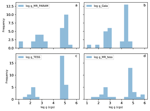
Figure 1: Distribution of $\log g$ for cooler stars in final sample. This was completed using: a) mass and radius derived by theoretical isochrones; b) Gaia parallaxes; c) directly from TIC; and d) mass and radius reports in TIC.

In the Fig. 1, we present the distribution of the $\log g$ for cool stars ($T_{\mathrm{eff}}$ ¡ 3950) as derived by each method. There are ten stars in the Lépine & Gaidos (2011) that are characterized as having $\log g$ ¡ 3.5 by all the above methods. As such, these are confidently classified as giant stars; we excluded these stars from the final list. There are also five stars for which the $\log g$ have different values using the Gaia parallax and TIC if available. Therefore, these targets were flagged as potential giants and will be followed with high caution when performing RV measurements.

2.7 Acquisition of new high-resolution observations

High-resolution spectra for the previously described list of 122 stars for which no high-resolution high-$S/N$ data were available, were requested in open time calls of an ESO proposal (program ID: 097.C-0561(A-B)), and then through a HARPS-N complementary proposal (program ID: A33TAC_7). The instruments used were HARPS, HARPS-N (Cosentino et al., 2012) mounted on the 3.58m Telescopio Nazionale Galileo at Roque de los Muchachos Observatory in La Palma (Canary Islands, Spain), and UVES (Dekker et al., 2000) spectrographs at Unit Telescope 2 of the VLT array.

Since M stars are faint in the optical, most of the M dwarfs identified as potential candidates were observed with UVES, mounted on the VLT. The choice of UVES as an instrument provides, just like HARPS, full coverage of the spectral optical domain, allowing the activity indicators to be covered. As an example, for a $V$=12.0, M2 star we obtained a $S/N$ of $\sim$ 15 at the Ca II H $\&$ K regions, and $S/N$ $\sim$100 at 600nm central wavelength.

Table 2: Summary of Data sources and number of spectra

	G and K type	M type	HARPS	HARPS-N	UVES
Archive	28	95	100	0	22
New Observation	78	44	78	44	42
Total	106	139	178	44	64

The final sample consists of stars observed from 3 to 8 May 2016 using HARPS, UVES UT2-Kueyen between April-July 2016, and using HARPS-N, between July-September 2016. For each target, at least two spectra were collected on different nights. In Table 2, a brief overview of the observations is presented. The average $S/N$ for spectra obtained by HARPS and HARPS-N is 210 and by UVES is 51 at mid-wavelength (around 550 nm).

2.8 Data Reduction and Cross-Correlation Function derivation

For HARPS and UVES, we collected all reduced, raw, and associated calibration-reduction spectra taken each night using the ESO archives. We performed the same data collection procedure for the 122 targets that were already observed at least twice using HARPS and UVES spectrographs, above the threshold of 210 for HARPS and HARPS-N and 51 for UVES. For HARPS-N and HARPS spectra data reduction, we used the latest version of the HARPS-N pipeline (DRS V3.8) using the Cross-Correlation Function, CCF technique with a template of G2, K5, and M2 masks (Pepe et al., 2002; Baranne et al., 1996). This pipeline provides the CCF’s full width at half maximum (FWHM), CCF’s bisector span inverse slope, and the Ca II activity index S and $Log(R^{\prime}_{HK})$ for F, G, and K stars.

In order to evaluate the presence of a second set of spectroscopic lines, we need to calculate the CCF in a wide window (see Sect. 3). We used the following procedure to calculate the CCFs in a range of $\rm 200\;km\;s^{-1}$ to ensure a contaminant CCF peak would not remain unnoticed.

The UVES data were reduced by a custom-made Python script that interfaces directly with ESO’s CPL (Common Pipeline Library) data reduction recipes for the UVES spectrograph (Martins & Figueira, 2017). This method permits two different approaches: i) run the red chain recipe that performs the whole reduction; and ii) perform a step-by-step data reduction using the individual data reduction recipes. We selected the latter approach as it allows finer control over the data reduction process.

It should be noted that when performing the flat-fielding of the science raw spectra, the UVES reduction recipes will remove the instrumental profile (i.e., blaze) information from the spectra. This means that the reduced spectra loses the information about the real flux, not allowing us to estimate the noise level at each wavelength. Due to this effect, the correction of the blaze function will give incorrect weights to the spectral lines closer to the edges when computing the CCF. To tackle this issue, we used the extracted, reduced, master-flat spectra for each order to reconstruct the blaze function, meaning the instrumental profile of the instrument on each order. These were constructed by performing a moving average over the extracted flat field for each order with a window of 100 pixels in the spectral space. This allows us to recover the instrumental profile, by smoothing the flat function over a 100-pixel region in the spectrum space to discard local defects (e.g., bad pixels). Each two-dimensional spectrum was then multiplied by the reconstructed blaze function to recalculate the spectra with the real flux.

To compute the CCF of each individual spectrum, we used the spectral masks from the HARPS DRS (Mayor et al., 2003). It should be noted that although they were originally built to be used with HARPS data, the wavelength coverage of both instruments is similar enough ([450-750]nm for UVES, against [378-691]nm for HARPS) that the same masks can be used. For each individual spectrum order and a given radial velocity $RV_{i}$, our implementation of the CCF is mathematically defined by

$$CCF_{order}(RV_{i})=\sum_{lines,order}\left(d_{line}\times\sum_{pixels}\left(f_{line,pix}\;F_{line,pix}\right)\right),$$ (5)

where $d_{line}$ is the depth of the selected line (from the binary mask); $pixels$ represents the list of spectral pixels covered by the selected line; $f_{line,pix}$ the fraction of the pixel that falls on the line; and $F_{line,pix}$ the flux of the line for each pixel (from the spectrum). Note that the $line$ parameter is dependent on $RV_{i}$, as it refers to the spectral line wavelength position for the given $RV_{i}$. The CCF value is then computed over a RV range centered on the expected RV of the system, yielding a plot such as the one presented in Figure 2.

3 Signature of stellar companions in the CCF

One of the goals of this study is to identify stars that are binaries or affected by the presence of a background star inside the fibre. For G and K type stars the presence of a contaminator can create a systematic RV signal of $\rm 10\;cm\;s^{-1}$ even in the extreme case when the difference in magnitude is of ten; this parasite signal can be larger than $\rm 1\;m\;s^{-1}$ if the difference in magnitude is less than eight (Cunha et al., 2013). For M type stars, a difference of magnitude between target and contaminant of eight, creates an effect of $\rm 10\;cm\;s^{-1}$ and a difference of magnitude between target and contaminant of six leads to an effect of $\rm 1\;m\;s^{-1}$ (Cunha et al., 2013). As such, a careful examination should be made to search for hints of companions.

There are several methods that can be used to check if the star has any detectable contaminations. Here we investigate using the CCF. The goal is to determine CCF’s pollution induced by a second star in the sky, close enough to contribute with light to the total collected in the fiber. This companion can be gravitationally bound or fortuitously aligned with the star. If the companion or companions exist and are bright enough, the presence of a second set of lines can create either a secondary correlation peak, if well-separated in RV from the target, or a change in the CCF line profile, if blended with the target. After calculating the CCFs in a wide window ($\rm 200\;km\;s^{-1}$), we compared the different CCFs obtained on each star for any anomaly in its usually ”Gaussian shape” as well as of variability in its profile. In the first approach, we searched for the characteristic double peak signature, and identified six targets, five of which are known binaries with significant CCF contamination. We considered a Gaussian-like shape with a CCF depth of at least 10% (an admittedly arbitrary value) to be a secondary peak. In Fig. 2, it is possible to see an example of double-line CCFs due to spectroscopic contamination. We include these targets with a signature of binary nature with ”Y+” flag in Table LABEL:result.

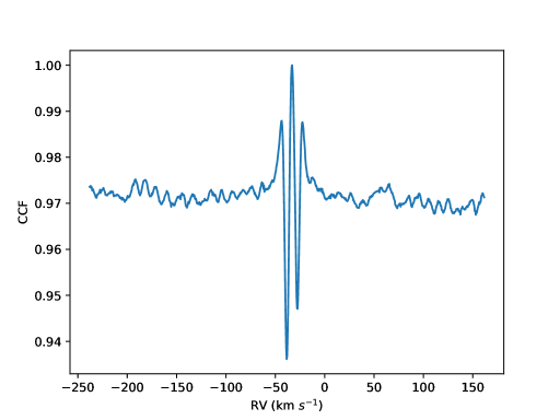
Figure 2: Example CCF of star with two significant peaks.

After this visual inspection procedure, we applied a more homogeneous criterion to identify stars on which a second component was present. We followed the method of Bouchy et al. (2016): after the derivation of CCFs, we shifted the reduced CCFs to a common RV value and mutually subtracted them. We then searched if there was a significant peak in the CCF residuals (see Fig. 3). The criteria for the absence of an additional peak is defined by

$$\sqrt{(S/N_{1})^{2}+(S/N_{2})^{2}}<\frac{1}{\sigma_{RMS}}.$$ (6)

Here the $S/N_{1}$ and $S/N_{2}$ are the median order signal-to-noise ratios of the CCFs, which are available in the reduced FITS headers; and $\sigma_{RMS}$ is the root mean square, RMS of the residual of the CCF difference. If the above condition is not met, then this means there is an additional source of scatter in the data. Equation 6 provides a systematic way of searching for the secondary peak on CCFs affected by contamination, provided we have at least two spectra. Stars for which our analysis satisfies the above condition are flagged with ”N”, otherwise the target contamination flag is set as ”Y”. The results are presented in Table LABEL:result.

In most cases, we did not find any significant hint of companion. Twenty-one stars have a companion and were discarded according to this criteria.

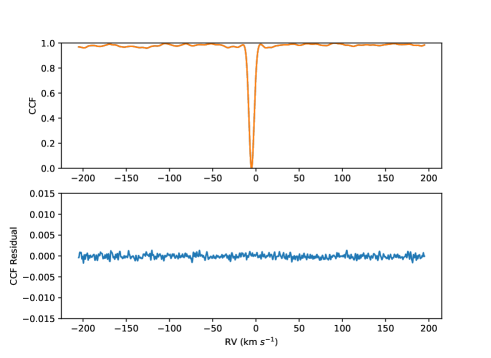
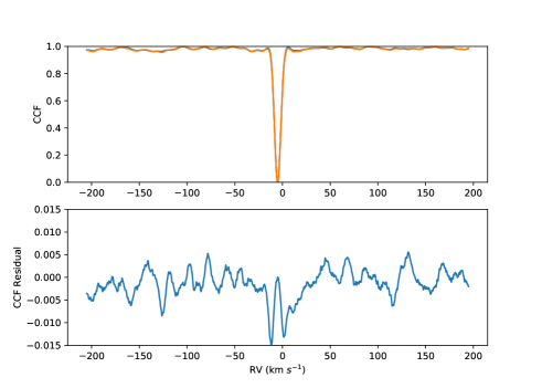
Figure 3: Two examples of normalized CCFs and residuals of stars. Upper panels: without signs of contamination; bottom panels: with hints of contamination.

4 Chromospheric activity indicator $log(R^{\prime}_{HK})$

Stellar activity related phenomena are known to produce significant RV signals. These can both induce noise in our data or produce coherent signals that can mimic the signature of an orbiting planet. Stellar active regions (e.g., dark spots and bright faculae) produce RV signals at the level of exoplanet orbital signals when they combine with stellar rotation. Stellar active regions also deform the CCF profile. As a consequence, they generate parasite RV signals (Meunier et al., 2010; Dumusque et al., 2014; Oshagh et al., 2017). As such, it is mandatory to track and characterize activity signals in order to disentangle the real exoplanet RV signal (e.g., Hatzes, 2013a; Queloz et al., 2001; Hatzes, 2013b; Santos et al., 2014; Robertson et al., 2014; Suárez Mascareño et al., 2017; Suárez Mascareño et al., 2018a).

To clear our sample from active stars, we used an activity indicator, $Log(R^{\prime}_{HK})$. We started by determining the S-index. This is a well-known quantity used for the first time in the long-term observations in the Mount Wilson stellar activity program (Vaughan et al., 1978; Duncan et al., 1991).

We used Ca II H $\&$ K lines and $R\&V$ continuum band-passes for S-index determination,

$$S=\alpha\frac{N_{H}+N_{K}}{N_{R}+N_{V}}\,.$$ (7)

The S-index measures the flux in the core of the line, normalized to the continuum band-passes. In this equation, $N_{H}$, $N_{K}$, $N_{R}$ and $N_{V}$ are the total flux in each band-pass and $\alpha$ is a calibration constant usually adjusted at 2.30 (Duncan et al., 1991). The 1.09 $\AA$ wide bands centred at 3933.664 $\AA$ and 3968.470 $\AA$ were used for K&H respectively. For V&R we used the 20 $\AA$ wide bands centred at 3901.070 $\AA$ and 4001.070 $\AA$, respectively.

To compare different stars’ activity, we need to remove the effect of the photospheric contribution and perform a normalization depending on the color index ($B-V$) that was introduced. The $log(R^{\prime}_{HK})$ has been defined by Noyes et al. (1984)

$$R^{\prime}_{HK}=1.34\times 10^{-4}\cdot C_{cf}(B-V)\cdot S-R_{phot}(B-V)\,,$$ (8)

where $C_{cf}(B-V)$ is the conversion factor (Noyes et al., 1984; Middelkoop, 1982). To derive $C_{cf}(B-V)$ we used the recent work of Suárez Mascareño et al. (2015), who calibrated these values in the range of B-V between 0.4 and 1.9:

$$log_{10}C_{cf}=0.668-1.270\cdot B-V+0.645\cdot B-V^{2}-0.443\cdot(B-V)^{3}.$$ (9)

Suárez Mascareño et al. (2015) call photospheric contribution to the H and K bandpasses $R_{phot}$ and we used the calibration defined as

$$R_{phot}=1.48\cdot 10^{-4}\cdot exp[-4.3658\cdot(B-V)].$$ (10)

Using these equations and measuring the fluxes in our spectra, we determined the S-index and $log(R^{\prime}_{HK})$. The HARPS and HARPS-N DRS measure the S-index and convert this into the chromospheric activity indicator $log(R^{\prime}_{HK})$. Both pipelines need $B-V$ and guess RV as input parameters. We used the $B-V$ values from the catalog data (e.g., Hipparcos) and the extracted RV from the CCFs. For HARPS-N, we used YAbI a web based access to the pipeline of HARPS-N. The pipeline provided the calibrated S-index and $log(R^{\prime}_{HK})$ for each spectrum in a similar way to HARPS.
For the stars observed with the UVES spectrograph, we corrected the RV shift using the RV’s determined by the CCFs and then calculated the $log(R^{\prime}_{HK})$.
We identified 43 stars with chromospheric activity higher than $-4.80$ dex, which usually is considered as the threshold for active stars (e.g., Vaughan & Preston, 1980). On the other hand, stars less active than this value are usually seen as stars with solar-like activity. We removed those active stars from our final sample. The derived activity values for all the stars are presented in Table LABEL:result and illustrated in Fig. 4.

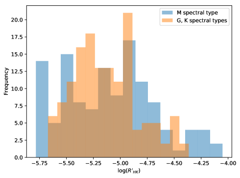
Figure 4: Derived $log(R^{\prime}_{HK})$ distribution for star sample.

5 Projected rotational velocity (v sin i)

Another important parameter affecting RV precision is the projected rotational velocity of the host star (v sin i). Assuming, for simplicity, that the spectral lines are resolved and have a Gaussian shape, RV precision is inversely proportional to the square root of the FWHM of the lines (e.g., Bouchy et al., 2001; Figueira, 2018). For a non-resolved spectral line, $\sigma_{\rm RV}\propto(v\sin i)^{1.5}$, if the other broadening mechanisms can be neglected in comparison to the rotational broadening.

We estimated the v sin i using the FWHM of the CCF and $B-V$ color and following the procedure described by several studies (e.g., Santos et al., 2002; Maldonado et al., 2017, with references therein) for HARPS data. We extended the calibration and used the stars that were observed with both HARPS and HARPS-N. Knowing that the instruments are very similar in design and in particular in resolution, a linear relationship was defined between the width of the CCF as measured by the two instruments. For CCF parameters like FWHM, we used the values produced by the previously mentioned standard pipelines of the two instruments. This allowed us to calculate the $v\sin i$ on HARPS-N for each FWHM. This calibration was performed independently for different masks corresponding to different spectral types (see Fig. 5). We followed the same procedure for UVES spectra as well. For the UVES spectra, we derived the width of the CCF and its associated uncertainty by using the tool provided by Martins & Figueira (2017), see Sect. 2.8. We used a sample of stars in common between HARPS and UVES in order to derive v sin i for the stars observed with UVES.
In Fig. 6, we plot the distribution of the v sin i measurements. The uncertainties on v sin i are derived by error propagation. We considered uncertainties on the CCF width for non-rotating stars and on the observed CCF width (Maldonado et al., 2017). For stars with more than one observation, we considered the standard deviation of the observed CCF width and the photon noise on the CCF in the error propagation equations. The mean value of the final uncertainties is of 0.47 $km\leavevmode\nobreak\ s^{-1}$, which is compatible with the work of Browning et al. (2010) and Maldonado et al. (2017). Uncertainties coming from simple error propagation are by construction underestimations and the method needs a deeper analysis on the uncertainties and dependencies on both other astrophysical parameters as well as the systematic errors coming from the simplified model applied to link the v sin i to the FWHM of the CCF (Maldonado et al., 2017; Browning et al., 2010; Reiners et al., 2018, and references therein). However, it is enough to detect the high rotation velocity stars as it is the aim of the paper. The results for v sin i are presented in Table LABEL:result. We reported values the v sin i ¡ 2.0 $km\leavevmode\nobreak\ s^{-1}$ as ”¡ 2.0 $km\leavevmode\nobreak\ s^{-1}$” because of the limited instrumental resolution. The FWHM of a spectrograph with R=100000 corresponds to $\sim$ 2.0 $km\leavevmode\nobreak\ s^{-1}$. As such, one cannot measure rotational velocity values smaller than this value. Most of the targets have low projected rotational velocity except three stars. Twenty-three targets were identified as having a high rotational velocity with v sin i ¿ 5.0 $km\leavevmode\nobreak\ s^{-1}$ and were removed from the final sample.

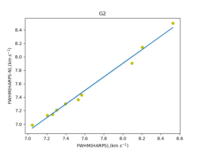
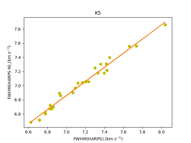
Figure 5: Calibration of FWHM examples in order to derive v sin i for common stars sampled in HARPS and HARPS-N data.

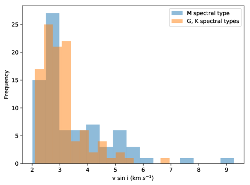
Figure 6: Derived v sin i distribution for star sample.

6 Complementary list for the known exoplanet systems

On top of the stars discussed above, we decided to give particular attention to the stars with known planets. In particular, we looked for systems that both satisfy our previous criteria and that could host an additional Earth-mass planet in the habitable zone. We applied the photon noise criteria and visibility on the known G, K, and M spectral type hosting exoplanets. As a source of known exoplanets we used the The Exoplanet Encyclopaedia and NASA Exoplanet Data Archive. For the stellar parameters we used the SWEET-CAT (Santos et al., 2013; Andreasen et al., 2017) to exclude giants ($\log g<4.1$ $cm\leavevmode\nobreak\ s^{-2}$) and select the stars of G, K, and M spectral types. For each confirmed exoplanet system, we determined the HZ defined by Selsis et al. (2007). Then we investigated the stability of an Earth-mass planet inside HZ using Hill-stability for circular orbits as well as orbits with the given eccentricity in the exoplanets catalogs. For these stars we did not apply activity criteria. We then applied the Eq. 24 from Gladman (1993) as stability criterion

$$\frac{a_{1}-a_{2}}{a_{1}}>2.40(\mu_{1}+\mu_{2})^{1/3},$$ (11)

to ten different orbits within the HZ (in regular steps of orbital separation). Here $\mu_{i}=m_{i}/m_{\star}$, $m_{i}$, and $m_{\star}$ are the mass of planets and star, $a_{i}$ is a semi-major axis, and i = 1, 2 for the two planets respectively. For each of them we checked the stability condition for a potential Earth-mass planet in a circular orbit. Our goal was to select and retain only those systems for which at least one of the tested orbits is stable.

On the other hand, for systems with planets in eccentric orbits we used Eq. 21 from Gladman (1993),

$$\left(\mu_{1}+\mu_{2}\frac{a_{1}}{a_{2}}\right)\left(\mu_{1}\gamma_{1}+\mu_{2}\gamma_{2}\sqrt{\frac{a_{2}}{a_{1}}}\right)^{2}>\alpha^{3}+3^{4/3}\mu_{1}\mu_{2}\alpha^{5/3},$$ (12)

where $\gamma_{i}=\sqrt{1-e^{2}}$, $\alpha=\mu_{1}+\mu_{2}$ and $e_{i}$ is the eccentricity. For the systems with more than one planet, each pair of planets was considered. By using the stable-orbits in the HZ of the system, we determined the Earth-mass planet orbital period in the innermost stable orbit in the most optimistic HZ using the generalized Kepler third law:

$$P/1yr=\sqrt{\frac{a^{3}/AU}{M_{\star}/M_{\sun}}}.$$ (13)

Then we estimated the semi-amplitude for RV variation (K) using Eq. 1. Table 3 lists the parameters for the known exoplanet systems with at least one stable orbit. However using Hill’s criterion can be risky because it is valid only for coplanar orbits (Gladman, 1993) and ignores the possibility of the existence of stable islands due to the secular resonances. Therefore we did not exclude any target from the our list based on this criterion. Further comprehensive analysis of each individual system is required to reach any firm conclusion.

Table 3: Nineteen known exoplanet systems with free stable orbit in HZ (C=satisfy with circular orbits, EC: satisfy considering eccentric orbits)

Star Name $T_{\mathrm{eff}}$ [K] $[Fe/H]$ $\log g$ [cm$s^{-2}$] Spectral type Period HZ [day] K$[cm\leavevmode\nobreak\ s^{-1}]$ Stability $log(R^{\prime}_{HK}$) and [data sources] HIP43587 5279 $\pm$ 62 0.33 $\pm$ 0.07 4.37 $\pm$ 0.18 G8 130.43 13 C -5.070 $\pm$ 0.012 [7] HIP98767 5584 $\pm$ 36 0.24 $\pm$ 0.05 4.37 $\pm$ 0.11 G8 179.46 12 C -5.09 [2] HIP57443 5629 $\pm$ 29 -0.29 $\pm$ 0.02 4.44 $\pm$ 0.03 G8 198.01 12 C -4.944 $\pm$ 0.010 [5] HIP64924 5577 $\pm$ 33 0.01 $\pm$ 0.05 4.34 $\pm$ 0.11 G8 179.06 12 C -4.920 $\pm$ 0.014 [1] HIP80337 5858 $\pm$ 18 0.03 $\pm$ 0.01 4.50 $\pm$ 0.03 G2 225.18 10 C 4.52 [2] HIP113357 5804 $\pm$ 36 0.20 $\pm$ 0.05 4.42 $\pm$ 0.07 G5 203.02 10 EC -4.963 $\pm$ 0.042 [3] HIP86796 5798 $\pm$ 33 0.32 $\pm$ 0.04 4.33 $\pm$ 0.08 G5 209.91 10 C -5.000 $\pm$ 0.032 [4] HIP40693 5402 $\pm$ 28 -0.06 $\pm$ 0.02 4.40 $\pm$ 0.04 K0 158.35 13 EC -4.898 $\pm$ 0.250 [4] HIP8102 5310 $\pm$ 17 -0.52 $\pm$ 0.01 4.46 $\pm$ 0.03 K0 187.37 13 C -4.886 $\pm$ 0.202 [8] HIP15510 5401 $\pm$ 17 -0.40 $\pm$ 0.01 4.40 $\pm$ 0.03 K0 177.95 14 EC -4.915 $\pm$ 0.016 [9] HIP99825 5099 $\pm$ 65 -0.30 $\pm$ 0.04 4.43 $\pm$ 0.13 K0 135.45 14 C -4.893 $\pm$ 0.060 [10] HIP3093 5182 $\pm$ 79 0.12 $\pm$ 0.05 4.40 $\pm$ 0.16 K0 135.5 14 C -5.02 [2] HIP16537 5049 $\pm$ 48 -0.15 $\pm$ 0.03 4.45 $\pm$ 0.09 K1 126.01 15 C -4.440 $\pm$ 0.021 [1] HIP10138 5114 $\pm$ 61 -0.29 $\pm$ 0.04 4.55 $\pm$ 0.13 K1 136.18 15 EC -4.702 $\pm$ 0.120 [11] HIP83043 3519 $\pm$ 150 -0.04 $\pm$ 0.10 4.76 $\pm$ 0.12 M1 27.79 32 C -5.016 [2] HIP24186 3550 $\pm$ 50 -0.89 – M1 33.4 46 EC -5.882 $\pm$ 0.051 [6] HIP85523 3334 $\pm$ 110 -0.23 $\pm$ 0.09 4.92 $\pm$ 0.21 M2 31.43 41 EC -4.967 $\pm$ 0.110 [6] HIP106440 3446 $\pm$ 110 -0.17 $\pm$ 0.09 4.83 $\pm$ 0.15 M3 24.24 38 EC -5.323 $\pm$ 0.030 [12] HIP70890 3050 $\pm$ 100 -0.03 5.0 M6 6.54 140 C -4.963 $\pm$ 0.009 [13]

• [1]: 192.C-0852(A), [2]: NASA Exoplanet Data Archive, [3]: 091.C-0271(A), [4]: 183.C-0972(A), [5]: (Gomes da Silva et al., 2014), [6]: 072.C-0488(E). [7]: 288.C-5010(A), [8]: 093.C-0062(A), [9]: 096.C-0053(A), [10]: 097.C-0021(A), [11]: 60.A-9700(G), [12]: 198.C-0838(A), [13]: 191.C-0505(A)

7 Stellar characterization and chemical abundance

Stellar parameters are not only crucial for accurate characterization of exoplanets but there is also increasing evidence that the characteristics of exoplanets are correlated to several host stars’ properties (e.g., Adibekyan et al., 2016; Mayor et al., 2004; Fischer & Valenti, 2005; Reffert et al., 2015). In recent studies, chemical abundance has provided useful constraints for planet structure and composition, and to investigate planet formation theories (e.g., Santos et al., 2017). For this aim, we derived stellar parameters ($T_{\mathrm{eff}}$: effective temperature, [Fe/H]: metallicity, $\log g$: surface gravity, and $\xi_{\mathrm{t}}$: microturbulence) and chemical abundances for all of the stars in the sample.

The stellar parameters and chemical abundances for G and K dwarfs are determined with the procedure described in Sousa (e.g. 2014); Adibekyan et al. (e.g. 2012c). In short, we first automatically measured the equivalent widths (EWs) of the spectral lines using the Automatic Routine for line Equivalent widths in stellar Spectra, ARES v2 code (Sousa et al., 2015) . For the more problematic elements we performed careful visual inspection of the determination of EWs. Then the spectroscopic parameters and chemical abundances were derived using the classical curve-of-growth analysis method forcing excitation and ionization equilibrium under assumption of local thermodynamic equilibrium (LTE). We used the grid of the ATLAS9 plane-parallel model of atmospheres (Kurucz, 1993) and the 2014 version of MOOG radiative transfer code (Sneden, 1973). The uncertainties of the stellar parameter and chemical abundances are also derived as in the references above. It is important to note that they represent the internal precision of the technique and not the absolute accuracies that can be significantly worse due to several factors as discussed in Hinkel et al. (e.g. 2016); Jofré et al. (e.g. 2017).

Abundances of the volatile elements, C and O, were only derived for a subsample of the stars and following the method of Delgado Mena et al. (2010); Bertran de Lis et al. (2015). As discussed in those works the derivation of abundances for these elements with the EW method and the lines employed here is only possible for unevolved stars with $T_{\mathrm{eff}}$$\gtrsim$ 5100 K. For Carbon, we measured the EWs of two atomic lines with ARES v2 code but under a visual inspection since the line at 5052 Å gets weaker as $T_{\mathrm{eff}}$ decreases. Given that the very few oxygen lines may be strongly blended, we choose to manually measure them with the task splot in Image Reduction and Analysis Facility , IRAF. The line at 6158 Å gets very weak for cooler stars and the forbidden line at 6300 Å is blended with Ni and CN lines (which become stronger as $T_{\mathrm{eff}}$ decreases). Then the abundances were derived using the 2014 version of MOOG as they were for the other elements.

In Figs. 7 and  8 we present dependence of the [X/Fe] abundance ratios on the stellar metallicity. The comparison is done for the large primary sample including stars with $\log g$ ¡ 4.1 $cm\leavevmode\nobreak\ s^{-2}$. For comparison, the HARPS sample of FGK dwarf stars from Adibekyan et al. (2012c) is plotted as well. The abundances of atomic Carbon and Oxygen for the HARPS sample stars were derived in Delgado Mena et al. (2010) and Bertran de Lis et al. (2015), respectively. Figure 7 shows that the two samples generally follow the same trend set by the Galactic chemical evolution. However, some discrepancies are apparent and worth mentioning. It seems that at metallicities above solar value Al and especially Si abundances relative to iron are higher for the current sample when compared to the HARPS sample stars. For the same metallicities, Ca and TiII seem to be under-abundant when compared to their HARPS counterparts. Most probably this is because many of the stars of the first sample are giant, evolved stars. Figure 8 shows that indeed, most of the Al- and Si-enhanced, and Ca- and TiII-poor stars are evolved stars with $\log g<3.5$ dex. Several studies observed such differences in chemical abundances between main-sequence dwarfs and evolved stars (e.g., Friel et al., 2003; Villanova et al., 2009; Adibekyan et al., 2015). These differences might have astrophysical origins (e.g., Tautvaišienė et al., 2005, as in the case of Sodium), they might be related to the spectroscopic analysis methods and use line-lists (e.g., Santos et al., 2009) and/or non-LTE effects, which are stronger for evolved stars (e.g., Bergemann et al., 2013). Some of the elements also show a dependence on effective temperature that has already been noticed and discussed in the literature (e.g. Gilli et al., 2006; Lai et al., 2008; Adibekyan et al., 2012c). These trends may be related to the stronger line blendings at low temperatures, deviations from excitation and/or ionization equilibrium, or an incorrect T-$\tau$ relationship in the adopted model atmospheres (see Adibekyan et al., 2012c, for more details and references)

Figure 7 shows that the most iron-poor stars are enhanced in $\alpha$ elements and probably belong to the Galactic thick disk (e.g., Adibekyan et al., 2013; Recio-Blanco et al., 2014). This is very interesting to note since it was found that planets orbiting iron-poor stars prefer the $\alpha$-enhanced ones (e.g., Haywood, 2009; Adibekyan et al., 2012a, b). Enhancement of the $\alpha$ elements, such as Mg and Si, relative to iron can play a very important role not only for the formation of planets, but also on the composition of the formed planets (Santos et al., 2017).
For the M dwarfs for which spectra were available, we used a modified version of the method and software developed by Neves et al. (2014) to $T_{\mathrm{eff}}$ and [Fe/H]. The $T_{\mathrm{eff}}$ scale was updated and its initial values were calculated as the average of the ($V-J$), ($V-H$), and ($V-K$) calibrations taken from Boyajian et al. (2012) . The corresponding errors were reported using Tables 5 and 6 in Neves et al. (2014).  The values are presented in Tables LABEL:stellar-param-table, LABEL:chemichal1, and LABEL:chemichal2. We presented $\log g$ using Eq. 3 and $T_{\mathrm{eff}}$using color calibrations where the sufficient spectra were not available and the targets were already discarded by the other criteria from the final list. The error bar for these targets were not calculated.

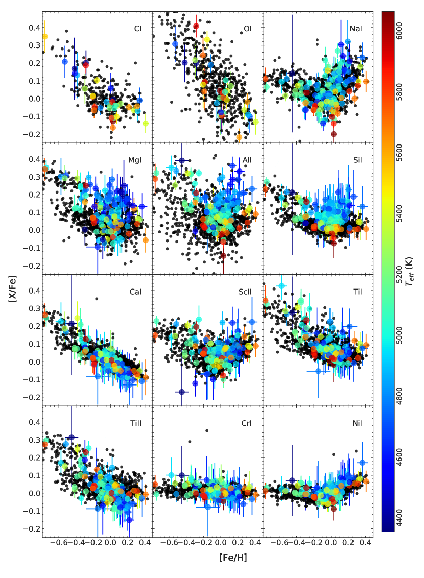
Figure 7: Abundance ratio [X/Fe] against stellar metallicity for current sample (color-coded by $T_{\mathrm{eff}}$) and for HARPS-sampled field stars (black).

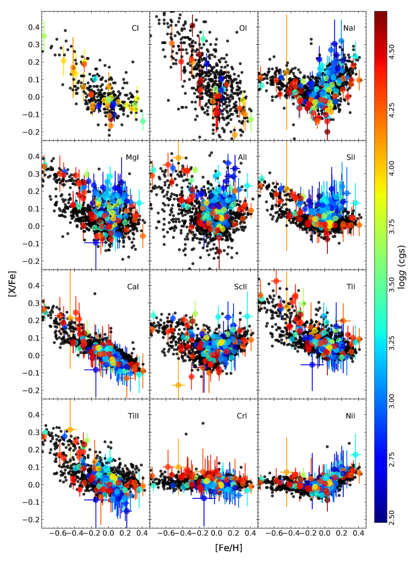
Figure 8: Abundance ratio [X/Fe] against stellar effective temperature for current sample (color-coded by $\log g$) and for HARPS-sampled field stars (black).

7.1 Composition of planetary building blocks

For a sample of 32 solar-type stars we derived abundances of the main rock-forming refractory (Mg, Si, and Fe) and volatile (O, C) elements. We used the model described in Santos et al. (2017) to compute the expected iron-to-silicate mass fraction (f_iron) and the water mass fraction (wf) in the planetary building blocks. The derived values of these quantities are presented in Table  4 and their distributions are shown in Fig. 9. The distribution of f_iron and wf are very similar to the distribution of the same quantities derived by Santos et al. (2017) for the Galactic thin disk stars in the solar neighborhood.

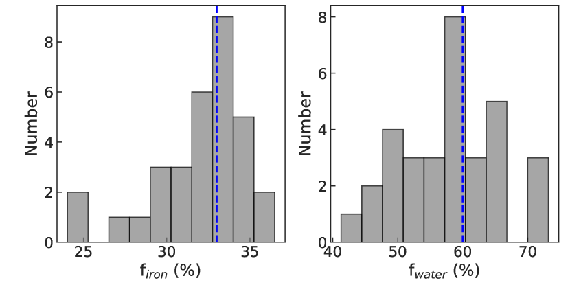
Figure 9: Expected iron and water mass fraction distributions of planetary building grains around sample stars. The values of these quantities derived for the solar system with our model are shown with dashed blue line.

Table 4: Iron-to-silicate and water mass fraction of planet building blocks. ($\star$ : host confirmed exoplanet)

star	$f_{iron}\leavevmode\nobreak\ [\%]$	$\textit{wf}\leavevmode\nobreak\ [\%]$
HIP13402	35.0 $\pm$ 3.1	58.1 $\pm$ 7.1
HIP16852	31.0 $\pm$ 2.0	57.3 $\pm$ 4.6
HIP22263	36.5 $\pm$ 1.3	59.6 $\pm$ 7.7
HIP23835	29.0 $\pm$ 1.2	73.1 $\pm$ 2.6
HIP43587$\star$	31.6 $\pm$ 3.0	46.5 $\pm$ 8.0
HIP64924$\star$	33.3 $\pm$ 1.8	49.3 $\pm$ 8.8
HIP77257	33.0 $\pm$ 1.1	58.5 $\pm$ 2.8
HIP83541	31.5 $\pm$ 2.6	47.4 $\pm$ 6.5
HIP95447	35.3 $\pm$ 2.8	48.7 $\pm$ 5.5
HIP98066	34.7 $\pm$ 1.6	51.9 $\pm$ 5.1
HIP98767$\star$	31.2 $\pm$ 2.1	49.4 $\pm$ 4.5
HIP101345	32.9 $\pm$ 1.0	59.3 $\pm$ 3.7
HIP101916	33.5 $\pm$ 1.9	56.2 $\pm$ 4.0
HIP113357$\star$	34.8 $\pm$ 2.0	41.3 $\pm$ 4.7
HIP37606	31.9 $\pm$ 1.4	57.8 $\pm$ 4.2
HIP107649	34.8 $\pm$ 1.9	50.8 $\pm$ 6.5
HIP86796$\star$	33.2 $\pm$ 2.0	55.1 $\pm$ 4.0
HIP114699$\star$	30.2 $\pm$ 1.1	66.1 $\pm$ 3.6
HIP29271	33.4 $\pm$ 1.8	61.4 $\pm$ 5.6
HIP1599	32.2 $\pm$ 1.4	61.7 $\pm$ 6.1
HIP8102$\star$	24.0 $\pm$ 1.8	66.6 $\pm$ 6.5
HIP10138$\star$	27.6 $\pm$ 1.7	64.0 $\pm$ 6.0
HIP15330	32.0 $\pm$ 1.9	60.1 $\pm$ 9.1
HIP15371	32.4 $\pm$ 1.6	70.8 $\pm$ 5.6
HIP38908	24.6 $\pm$ 1.3	73.2 $\pm$ 3.4
HIP40693$\star$	32.6 $\pm$ 1.6	53.8 $\pm$ 8.1
HIP56452	29.7 $\pm$ 2.0	66.0 $\pm$ 6.9
HIP57443	28.6 $\pm$ 1.6	65.8 $\pm$ 6.6
HIP81300	34.1 $\pm$ 2.3	51.2 $\pm$ 9.2
HIP110109	33.0 $\pm$ 1.2	58.7 $\pm$ 7.4

8 Stellar rotational period estimation for M dwarfs

The rotation period of M dwarfs can be of the same order of magnitude as the period of a planet in the HZ. The presence of active regions on M dwarfs can thus produce an RV signal that can mimic the signal produced by an Earth-mass exoplanet inside the HZ or at any harmonic of the rotation period (e.g., Boisse et al., 2009).

We derived the expected rotational period of M dwarfs using activity-rotation relationships as a first estimation. Several studies show a significant correlation between the activity and rotation for M dwarfs (e.g., Suárez Mascareño et al., 2018b; Astudillo-Defru et al., 2017; Suárez Mascareño et al., 2016). We used Eq.1 and Table 1 from Suárez Mascareño et al. (2015) for the rotational period determination from the $log(R^{\prime}_{HK})$. In Table 5, we list the rotational period estimated in this way, as well as the orbital period corresponding to the inner boundary of the HZ for our sample of M dwarfs. We derived the error using the standard error propagation of the input parameters’ errors. For low-activity stars ($log(R^{\prime}_{HK})$ ¡ -4.80), the rotation periods shows a large dispersion, specially for the early M spectral types. Therefore, in order to take into account the actual dispersion of the data points in Fig. 12 from Suárez Mascareño et al. (2018b), we considered an uncertainty in the rotation period inflated by a factor of three.

We are aware that the rotation periods obtained in this way are a first-order estimation. Although the statistical strength of the relationship for the purpose of this study is sufficient enough, we did not exclude any target from the final list based on this criterion. There are some stars for which extreme caution is necessary because the rotational period of the stars are very close to the HZ inner edge’s orbital period. For these targets distinguishing the planetary signal from RV variations of stars due to its rotation will be quite challenging. The measurements can be improved in the future studies using either photometric or spectroscopic methods.

Table 5: Sample of M dwarf in final list with rotational periods and HZ parameters.

Star Name	$P_{rot}$ [day]	Stellar mass [$M_{\sun}$] and Reference	$P_{inner}$[day]	HZ [AU]
HIP439	79 $\pm$ 6	0.39$\pm$0.03 [1]	25$\pm$1	[ 0.12 , 0.32 ]
HIP1242	192 $\pm$ 8	0.14 [2]	12	[ 0.05 , 0.14 ]
HIP22627	64 $\pm$ 6	0.37$\pm$0.06 [3]	20$\pm$2	[ 0.1 , 0.28 ]
HIP23708	33 $\pm$ 5	0.59$\pm$0.02 [4]	55$\pm$1	[ 0.24 , 0.61 ]
HIP29295	29 $\pm$ 5	0.58$\pm$0.06 [1]	41$\pm$2	[ 0.19 , 0.5 ]
HIP40239	161 $\pm$ 8	0.61 [2]	49	[ 0.22 , 0.57 ]
HIP42748	81 $\pm$ 6	0.45$\pm$0.05 [4]	60$\pm$3	[ 0.23 , 0.59 ]
HIP45908	31 $\pm$ 5	0.55$\pm$0.03 [1]	38$\pm$1	[ 0.18 , 0.46 ]
HIP51317	46 $\pm$ 5	0.44$\pm$0.03 [1]	26$\pm$1	[ 0.13 , 0.34 ]
HIP53020	88 $\pm$ 6	0.26$\pm$0.02 [1]	14$\pm$1	[ 0.07 , 0.2 ]
HIP62452	104 $\pm$ 7	0.32$\pm$0.02 [1]	16$\pm$1	[ 0.09 , 0.23 ]
HIP65859	30 $\pm$ 5	0.53$\pm$0.03 [1]	34$\pm$1	[ 0.17 , 0.43 ]
HIP67164	80 $\pm$ 6	0.42$\pm$0.06 [5]	14$\pm$1	[ 0.09 , 0.23 ]
HIP71253	85 $\pm$ 6	0.28$\pm$0.02 [1]	15$\pm$1	[ 0.08 , 0.21 ]
HIP85523	38 $\pm$ 5	0.35$\pm$0.03 [1]	21$\pm$1	[ 0.1 , 0.27 ]
HIP86214	35 $\pm$ 5	0.27$\pm$0.02 [1]	15$\pm$1	[ 0.08 , 0.21 ]
HIP86287	73 $\pm$ 6	0.45$\pm$0.03 [1]	28$\pm$1	[ 0.14 , 0.36 ]
HIP87937	73 $\pm$ 6	0.16$\pm$0.01 [1]	9$\pm$1	[ 0.04 , 0.12 ]
HIP88574	46 $\pm$ 5	0.48$\pm$0.03 [1]	30$\pm$1	[ 0.15 , 0.38 ]
HIP92403	30 $\pm$ 5	0.17$\pm$0.01 [1]	11$\pm$1	[ 0.05 , 0.14 ]
HIP93069	49 $\pm$ 5	0.53 [2]	59	[ 0.24 , 0.62 ]
HIP93101	28 $\pm$ 4	0.43$\pm$0.05 [4]	51$\pm$3	[ 0.2 , 0.52 ]
HIP99701	26 $\pm$ 4	0.59 [2]	42	[ 0.2 , 0.51 ]
HIP106440	52 $\pm$ 5	0.45$\pm$0.03 [1]	28$\pm$1	[ 0.14 , 0.35 ]
HIP113020	112 $\pm$ 7	0.34$\pm$0.02 [1]	18$\pm$1	[ 0.09 , 0.25 ]
HIP115332	44 $\pm$ 5	0.4$\pm$0.02 [1]	20$\pm$1	[ 0.1 , 0.28 ]
HIP67155	38 $\pm$ 5	0.5$\pm$0.03 [1]	29$\pm$1	[ 0.14 , 0.37 ]

• [1]: Neves et al. (2013), [2]: Gaidos et al. (2014), [3]: Mann et al. (2015), [4]: Mints & Hekker (2017), [5]: Gaidos & Mann (2014)

9 Summary and conclusion

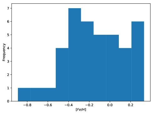
Figure 11: [Fe/H] distribution for final selected sample of stars where metallically values are available.

We present a detailed spectroscopical characterization of a sample of bright stars that are suitable targets for a precise RV planet search program focused on Earth-mass planets in their hosts habitable zone using ESPRESSO. To build this sample, we used new and archival high-resolution spectroscopic data. We screened a large sample of G, K, and M stars for visibility, spectroscopic contamination, chromosphere activity using $log(R^{\prime}_{HK})$, projected rotational velocity using v sin i, stellar parameters, and chemical abundances. After considering previous criteria, for the known host planetary systems we investigated the availability of a free, stable orbit for an Earth-mass planet inside the HZ.
Twenty-seven stars were discarded according to the signature of stellar companions in CCF criteria. Forty-three stars with high activity $log(R^{\prime}_{HK})$ ¿ -4.80 were excluded from the list due to the expected large activity-induced RV variations. We identified twenty-three stars with v sin i ¿ 5.0 $km\leavevmode\nobreak\ s^{-1}$ and excluded them from the final list. The list of the 45 best targets is presented in Table 6. For the known host planetary systems which were described in Sect. 6, nineteen best candidates are presented in Table 3. Five G, fifteen K, and twenty-seven M spectral type stars have $V$ between 3.49 and 11.94. Figures 10 and 11 present the distribution of [Fe/H] for forty stars with available chemical abundance values.

When performing our study we realized that many bright, main-sequence GKM stars did not have sufficiently high $S/N$ spectra in the ESO archive to allow spectroscopic analysis. The spectra obtained by us were made available immediately, and the reduced spectra, made available now, can be of interest to a wide range of studies. All the spectra are available for download from the ESO archive and also from our Porto data server for the case of HARPS-N observations.
Concerning the final target list, applying the criteria on spectroscopic contamination, stellar activity, and chromospheric activity levels, and discarding evolved stars by a direct or indirect assessment of the log$g$, led us to discard a large fraction of the stars. At the end of the selection steps, we retained only $\sim$45 of the $\sim$249 stars originally surveyed spectroscopically. This selection, which was devised to be independent of spectral type in any other aspect than photon noise, let to a catalog that is composed of roughly of 60% of M dwarfs. This is the first study that leads to the conclusion that, even when trying to be as independent as possible of spectral-type biases, when focusing on objective criteria such as photon noise and signal detectability from first principle, M dwarfs emerge as optimal RV targets, even at optical wavelengths.

Most of the stars (27) in the final list are of M spectral type. M dwarfs are good candidates not only for gravitational RV detection because of their relativity low mass, but also for having a closer HZ. Hypothetical planets around M dwarfs would have relatively shorter orbital periods, making it is easier to cover their orbital period. However M dwarfs with rotational periods close to the orbital period of an Earth-class planet in their HZ will be considered as of lower priority for observations. The sample of M dwarfs in our final list consists mostly of early-type and late-type spectral sub-types with very few in the intermediate sub-types. M dwarfs are not a homogeneous class of stars and there are many intermediate M dwarfs in this magnitude regime (see Fig. 5 in Figueira et al., 2016), so this came probably from statistical fluctuations arising from small number statistics. It should be mentioned that the temperature of the M dwarfs scatter over a few hundreds of kelvins in the different catalogs therefore we cannot compare the parameters in the the sub-spectral M dwarfs. The effective temperature determination of M dwarfs is affected by an uncertainty at the level of 100 K. As such, a detailed spectral type assignment based on effective temperatures is impossible, and we warn the reader against an over-interpretation of the data.

We considered stars for which the photon noise allowed the detection of an Earth-class planet inside the HZ. In the absence of sources of error other than the photon noise, an Earth-class planet is detectable in almost all of the candidates with orbital periods of $\approx$ 6 to $\approx$ 223 days by assuming the expected RV precision of $\rm 10\;cm\;s^{-1}$. Eighty percent of the ESPRESSO GTO is dedicated to exoplanet searches and one-third of this time is allocated to the blind RV survey (65 nights). By considering 9 hours as an average of night duration, an average of 100 data points in order to cover the orbital periods and 15-minute exposure time, we can intensively observe around 23 targets in this survey.
The composition of the planetary building block analysis suggests that the potential terrestrial planets orbiting the majority of these stars will have an iron core-size similar to that of the Earth, but will have a lower fraction of water content. It is also interesting to note that (based only on the chemistry of the host stars) terrestrial planets with very different compositions (e.g., core size) and water content when compared to the solar system, are also expected to be detected around some of the targets. Here we should note that the f_iron and wf derived with this model might not necessarily be exactly the same as the water content and core size of planets around the target stars (see Santos et al., 2017). These quantities are only indicative of the content of water in the protoplanetary disk and the iron-to-silicate ratio that might be translated into a core-to-mantle ratio.
Presently there is no clear indication if the presence of close-in planets (that have been detected e.g., with HARPS) is indicative of the presence of low-mass planets in the habitable zone. On one side, we know from Kepler data that some planetary systems are compact and dynamically full (Fabrycky et al., 2014). If this is a general feature, then the presence of close-in planets could be a positive indication of the presence of planets further out (whatever their mass). Since a giant planet in the HZ of such systems would already have been detected with HARPS, planets in the HZ should be rather small. On the other side, we know from the only confirmed Earth-like planet in the HZ (the Earth itself), that the absence of close-in planets is compatible with the presence of a low-mass planet in the HZ. Finally there are indications, from planet formation models, that the absence of close-in planets could be positively correlated with the presence of low-mass planets in the HZ (Alibert et al., in prep). Since there is no clear consensus on the correlation between the presence of already detected planets and the probability of having a planet in the HZ, we decided to include both types of stars (with or without already known planets) in our target list.

Figure 10: Visual magnitude vs $T_{\mathrm{eff}}$ [K] for final selected sample of stars

All derived parameters for the whole sample are presented in Table LABEL:result for our new observation and archives respectively. We derived the stellar parameters and chemical abundances for this sample of stars (Tables LABEL:stellar-param-table, LABEL:chemichal1, and LABEL:chemichal2) where it was possible.

Table 6: Forty-five best final targets for RV observation

Name	R.A [hh:mm:ss]	Dec [∘:′:′′]	v sin i [km $s^{-1}$]	$log(R^{\prime}_{HK})$	$\log I_{H\alpha_{index}}$	$V$	Sp Type
HIP86796	17 44 08.7	-51 50 00.9	2.95 $\pm$ 0.90	-5.15 $\pm$ 0.01	-1.37 $\pm$ 0.07	5.12	G5
HIP83541	17 04 27.8	-28 34 55.3	¡ 2.0	-5.02 $\pm$ 0.01	-1.43 $\pm$ 0.01	6.59	G8
HIP57443	11 46 32.2	-40 30 04.8	¡ 2.0	-4.88 $\pm$ 0.01	-1.49 $\pm$ 0.06	4.89	G8
HIP64924	13 18 25.0	-18 18 31.0	¡ 2.0	-4.91 $\pm$ 0.01	-1.45 $\pm$ 0.01	4.74	G8
HIP40693	08 18 23.8	-12 37 47.2	¡ 2.0	-4.94 $\pm$ 0.01	-1.46 $\pm$ 0.09	5.95	G8
HIP41926	08 32 52.2	-31 30 09.7	–	-4.91 $\pm$ 0.01	-1.43 $\pm$ 0.10	6.38	K0
HIP15510	03 19 53.2	-43 04 17.6	–	-5.00 $\pm$ 0.01	-1.45 $\pm$ 0.01	4.26	K0
HIP8102	01 44 05.1	-15 56 22.4	–	-4.90 $\pm$ 0.01	-1.44 $\pm$ 0.07	3.49	K0
HIP19849	04 15 17.6	-07 38 40.4	¡ 2.0	-4.92 $\pm$ 0.01	-1.41 $\pm$ 0.01	4.43	K1
HIP99825	20 15 16.6	-27 01 57.1	¡ 2.0	-4.96 $\pm$ 0.01	-1.41 $\pm$ 0.01	5.73	K1
HIP56452	11 34 30.0	-32 50 00.0	–	-4.83 $\pm$ 0.04	-1.44 $\pm$ 0.10	5.96	K1
HIP3765	00 48 22.5	+05 17 00.2	–	-4.93 $\pm$ 0.01	-1.41 $\pm$ 0.01	5.74	K2
HIP99461	20 11 11.6	-36 05 50.6	¡ 2.0	1.50	-1.41 $\pm$ 0.02	5.32	K2
HIP12114	02 36 03.8	+06 53 00.1	2.00 $\pm$ 0.27	-4.96 $\pm$ 0.01	-1.38 $\pm$ 0.04	5.79	K2
HIP23311	05 00 48.7	-05 45 03.5	¡ 2.0	-5.00 $\pm$ 0.01	-1.39 $\pm$ 0.01	6.22	K3
HIP16711	03 35 00.5	-48 25 11.6	¡ 2.0	-5.09 $\pm$ 0.01	-1.52 $\pm$ 0.01	8.57	K4
HIP108870	22 03 17.4	-56 46 47.3	¡ 2.0	-4.80 $\pm$ 0.01	-1.34 $\pm$ 0.07	4.69	K4
HIP85647	17 30 11.2	-51 38 13.0	2.64 $\pm$ 0.36	-5.12 $\pm$ 0.02	-1.53 $\pm$ 0.04	9.58	K7
HIP40239	08 13 08.5	-13 55 01.0	4.89 $\pm$ 0.23	-5.65 $\pm$ 0.25	-1.39 $\pm$ 0.07	9.38	M0
HIP29295	06 10 34.6	-21 51 52.4	2.61 $\pm$ 0.41	-4.90 $\pm$ 0.01	-1.51 $\pm$ 0.02	8.15	M1
HIP439	00 05 24.2	-37 21 25.3	¡ 2.0	-5.47 $\pm$ 0.01	-1.36 $\pm$ 0.02	8.56	M1
HIP42748	08 42 44.5	+09 33 24.4	2.67 $\pm$ 0.72	-5.48 $\pm$ 0.10	-1.39 $\pm$ 0.02	9.62	M1
HIP45908	09 21 37.7	-60 16 55.1	2.32 $\pm$ 0.65	-4.94 $\pm$ 0.01	-1.46 $\pm$ 0.02	9.49	M1
HIP93101	18 58 00.1	+05 54 29.8	2.44 $\pm$ 0.65	-4.86 $\pm$ 0.01	-1.46 $\pm$ 0.02	9.22	M1
HIP93069	18 57 30.6	-55 59 30.6	¡ 2.0	-5.19 $\pm$ 0.01	–	8.86	M1
HIP23708	05 05 47.4	-57 33 13.8	¡ 2.0	-4.96 $\pm$ 0.01	-1.42 $\pm$ 0.05	9.11	M2
HIP51317	10 28 55.6	+00 50 28.0	2.28 $\pm$ 0.20	-5.16 $\pm$ 0.02	-1.41 $\pm$ 0.01	9.65	M2
HIP86287	17 37 53.3	+18 35 29.7	2.63 $\pm$ 0.63	-5.43 $\pm$ 0.01	-1.50 $\pm$ 0.02	9.62	M2
HIP88574	18 05 07.6	-3 01 52.6	2.47 $\pm$ 0.29	-5.16 $\pm$ 0.01	-1.51 $\pm$ 0.02	9.37	M2
HIP106440	21 33 34.0	-49 00 32.0	2.09 $\pm$ 0.26	-5.23 $\pm$ 0.01	-1.48 $\pm$ 0.02	8.66	M2
HIP65859	13 29 59.7	+10 22 38.3	2.55 $\pm$ 0.20	-4.91 $\pm$ 0.01	-1.50 $\pm$ 0.02	9.05	M2
HIP99701	20 13 53.3	-45 09 50.4	¡ 2.0	-4.84 $\pm$ 0.06	-1.46 $\pm$ 0.02	7.97	M2
HIP67155	13 45 42.7	+14 53 42.2	–	-5.04 $\pm$ 0.01	-1.44 $\pm$ 0.01	8.46	M2
HIP85523	17 28 39.9	-46 53 42.2	2.59 $\pm$ 0.34	-5.05 $\pm$ 0.01	-1.22 $\pm$ 0.03	9.38	M3
HIP71253	14 34 16.8	-12 31 10.7	2.83 $\pm$ 0.51	-5.51 $\pm$ 0.01	-1.43 $\pm$ 0.04	11.32	M4
HIP1242	00 15 28.1	-16 08 01.4	4.30 $\pm$ 0.27	-5.68 $\pm$ 0.21	-1.38 $\pm$ 0.04	11.49	M6
HIP53020	10 50 52.1	+06 48 29.7	4.92 $\pm$ 0.22	-5.53 $\pm$ 0.10	-1.43 $\pm$ 0.10	11.64	M6
HIP87937	17 57 48.5	+04 41 31.0	–	-5.42 $\pm$ 0.01	-1.32 $\pm$ 0.07	9.54	M6
HIP92403	18 49 49.3	-23 50 10.3	5.20 $\pm$ 0.91	-4.91 $\pm$ 0.02	-0.98 $\pm$ 0.01	10.37	M6
HIP115332	23 21 37.5	+17 17 26.1	4.94 $\pm$ 0.23	-5.13 $\pm$ 0.20	-1.37 $\pm$ 0.05	11.70	M6
HIP22627	04 52 05.7	+06 28 35.7	3.82 $\pm$ 0.80	-5.35 $\pm$ 0.04	-1.39 $\pm$ 0.03	11.94	M6
HIP62452	12 47 56.7	+09 45 05.2	4.30 $\pm$ 0.24	-5.63 $\pm$ 0.10	-1.41 $\pm$ 0.01	11.39	M6
HIP113020	22 53 16.7	-14 15 49.0	2.75 $\pm$ 1.03	-5.67 $\pm$ 0.02	-1.47 $\pm$ 0.01	10.16	M6
HIP67164	13 45 50.7	-17 58 05.3	2.52 $\pm$ 0.25	-5.48 $\pm$ 0.04	–	11.81	M6
HIP86214	17 37 03.7	-44 19 08.7	3.42 $\pm$ 0.79	-4.99 $\pm$ 0.01	-1.44 $\pm$ 0.05	10.94	M7

Appendix A $H_{\alpha}$ Index

On top of the $log(R^{\prime}_{HK})$ index, we also computed, where it was possible for all our stars, an activity index based on the $H_{\alpha}$ line. The activity characterization of M dwarfs is made more difficult than for G and K counterparts due to the comparatively lower flux in the wavelength region corresponding to the Ca II H $\&$ K. Fortunately, several alternatives exist in the optical domain. It was demonstrated that an efficient activity indicator is $H_{\alpha}$, which correlates very well with the S index (Gomes da Silva et al. 2011). The $H_{\alpha}$ index is a well known and widely used chromospheric indicator (Kuerster et al. 2003; Bonfils et al. 2007). Further to the analysis of the $log(R^{\prime}_{HK})$ index, we also defined a homogenized $H_{\alpha}$ index similar to Boisse et al. (2009) but using a broader central band as proposed by Pasquini & Pallavicini (1991) in order to be more sensitive to chromospheric activity contribution (Gomes da Silva et al. 2014).

We computed the index as described in Boisse et al. (2009):

$$H\alpha_{index}=\frac{F_{H\alpha}}{F_{1}+F_{2}},$$ (14)

with $F_{H\alpha}$ sampling the $H_{\alpha}$ line, and the $F_{1}$ and $F_{2}$ as the continuum on both sides of the line. The $H_{\alpha}$ line is centered on 6562.808 $\AA$ with 1.6 $\AA$ wide and continuum $F_{1}$ and $F_{2}$, integrated over [6545.495, 6556.245 $\AA$] and [6575.934, 6584.684 $\AA$], respectively. Each spectrum is corrected for RV shift by its RV measurement by the CCFs. The error was extracted based on the measurement of flux computed by the pipelines and using error propagation. The $H\alpha_{index}$ as defined in this way is a good indicator to measure activity variation over time for a star. However, it can not be used to compare stars with different spectral types. There is a significant correlation between $H\alpha_{index}$ and $B-V$ that needs to be corrected in order to make $H\alpha_{index}$ compatible between different stars (Cincunegui et al. 2007). Here we follow a calibration extracted by Gomes da Silva et al. (2014) and extended it for the $B-V>1.2$ in order to calibrate $H\alpha_{index}$ and determine $\log I_{H\alpha_{index}}$ (see Table LABEL:result). The average value of our calibrated $\log H_{\alpha}$ index, $\log I_{H\alpha_{index}}$ is -1.460. As seen from Fig. 12, most stars have values close to -1.460, with only 15 stars having values above -1.150. We note that 14 stars out of these “highly active stars” had already been identified and screened out using the $log(R^{\prime}_{HK})$, which shows the strong correlation between the two indicators.

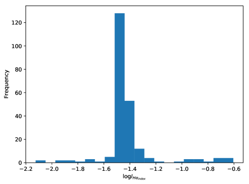
Figure 12: Derived $\log I_{H\alpha_{index}}$ distribution for sample stars.

Appendix B Tables.

1]

Table 7: Derived parameters for the first sample stars

Target	v sin i [km $s^{-1}$]	$log(R^{\prime}_{HK})$	$\log I_{H\alpha_{index}}$	Contamination	Program ID	$V$	Spectral-type
HIP93203	25.63 $\pm$ 0.55	-4.74 $\pm$ 0.01	–	N	[96],[97],[98]	5.27	G0
HIP115623	80.42 $\pm$ 0.93	-4.57 $\pm$ 0.01	-1.37 $\pm$ 0.02	–	[96],[97],[98]	4.42	G0
HIP23693	20.16 $\pm$ 0.35	-4.33 $\pm$ 0.01	-1.44 $\pm$ 0.03	N	[88],[89]	4.71	G0
HIP16852	3.36 $\pm$ 0.20	-5.24 $\pm$ 0.01	-1.50 $\pm$ 0.05	N	[39],[27]	4.30	G0
HIP1599	¡ 2.0	-4.89 $\pm$ 0.01	-1.48 $\pm$ 0.06	N	[81],[82]	4.23	G0
HIP38908	¡ 2.0	-4.89 $\pm$ 0.01	-1.48 $\pm$ 0.04	N	[81],[82]	5.59	G0
HIP77257	2.73 $\pm$ 0.21	-4.93 $\pm$ 0.01	-1.48 $\pm$ 0.07	N	[96],[97],[98]	4.42	G2
HIP22263	3.21 $\pm$ 0.22	-4.52 $\pm$ 0.01	-2.44 $\pm$ 0.01	N	[2],[5],[40]	5.50	G2
HIP107649	¡ 2.0	-5.10 $\pm$ 0.01	-1.39 $\pm$ 0.01	N	[43]	5.57	G2
HIP15371	¡ 2.0	-4.83 $\pm$ 0.01	-1.48 $\pm$ 0.10	N	[87]	5.24	G2
HIP58576	2.87 $\pm$ 0.92	-5.00 $\pm$ 0.04	-1.43 $\pm$ 0.09	N	[27]	5.54	G2
HIP110109	¡ 2.0	-4.89 $\pm$ 0.01	-1.49 $\pm$ 0.05	N	[82]	5.36	G2
HIP101916	4.42 $\pm$ 0.43	-5.00 $\pm$ 0.01	-1.49 $\pm$ 0.02	N	[96],[97],[98]	5.07	G5
HIP22449	19.92 $\pm$ 2.09	-4.67 $\pm$ 0.01	-1.47 $\pm$ 0.01	–	[34],[56]	3.19	G5
HIP23835	2.36 $\pm$ 0.31	–	-1.48 $\pm$ 0.01	N	[50],[13]	4.91	G5
HIP95447	–	-5.19 $\pm$ 0.01	-1.46 $\pm$ 0.04	N	[70],[47],[23]	5.17	G5
HIP98767$\star$	2.39 $\pm$ 0.82	-5.12 $\pm$ 0.01	-1.44 $\pm$ 0.09	N	[72]	5.73	G5
HIP101345	2.33 $\pm$ 0.25	-5.00 $\pm$ 0.01	-1.48 $\pm$ 0.01	N	[46],[11]	5.66	G5
HIP113357$\star$	2.47 $\pm$ 0.93	-4.93 $\pm$ 0.01	-1.46 $\pm$ 0.01	N	[64]	5.45	G5
HIP37853	–	-5.09 $\pm$ 0.01	-1.47 $\pm$ 0.02	Y+	[80]	5.36	G5
HIP86796$\star$	2.95 $\pm$ 0.90	-5.15 $\pm$ 0.01	-1.37 $\pm$ 0.07	N	[43]	5.12	G5
HIP15330	¡ 2.0	-4.55 $\pm$ 0.01	-1.45 $\pm$ 0.06	N	[85],[86]	5.53	G5
HIP38140	5.14 $\pm$ 0.24	-4.89 $\pm$ 0.01	-1.50 $\pm$ 0.01	N	[96]	6.55	G8
HIP77512	5.20 $\pm$ 0.65	-4.78 $\pm$ 0.01	-1.49 $\pm$ 0.09	N	[98]	4.59	G8
HIP98066	3.39 $\pm$ 0.61	-5.00 $\pm$ 0.01	-1.47 $\pm$ 0.05	N	[96]	4.70	G8
HIP64924$\star$	¡ 2.0	-4.91 $\pm$ 0.01	-1.45 $\pm$ 0.01	N	[46],[11]	4.74	G8
HIP83541	¡ 2.0	-5.02 $\pm$ 0.01	-1.43 $\pm$ 0.01	N	[11]	6.59	G8
HIP37606	2.49 $\pm$ 0.34	-5.15 $\pm$ 0.01	-1.47 $\pm$ 0.01	N	[61],[36]	5.04	G8
HIP29271	¡ 2.0	-4.97 $\pm$ 0.01	-1.47 $\pm$ 0.01	N	[69]	5.08	G8
HIP40693$\star$	¡ 2.0	-4.94 $\pm$ 0.01	-1.46 $\pm$ 0.09	N	[46],[81]	5.95	G8
HIP57443	¡ 2.0	-4.88 $\pm$ 0.01	-1.49 $\pm$ 0.06	N	[46],[87]	4.89	G8
HIP99240	2.36 $\pm$ 0.64	-5.04 $\pm$ 0.01	-1.46 $\pm$ 0.05	N	[94]	3.55	G8
HIP22319	2.47 $\pm$ 0.28	-4.93 $\pm$ 0.01	-1.46 $\pm$ 0.01	N	[96],[97],[98]	6.51	K0
HIP83688	3.94 $\pm$ 0.52	-4.94 $\pm$ 0.01	-1.51 $\pm$ 0.06	N	[96],[97],[98]	6.38	K0
HIP43587$\star$	2.17 $\pm$ 0.28	-5.06 $\pm$ 0.01	-1.42 $\pm$ 0.01	N	[37]	5.96	K0
HIP41926	–	-4.91 $\pm$ 0.01	-1.43 $\pm$ 0.10	N	[43]	6.38	K0
HIP15510	–	-5.00 $\pm$ 0.01	-1.45 $\pm$ 0.01	N	[43]	4.26	K0
HIP114699$\star$	¡ 2.0	-5.13 $\pm$ 0.01	-1.43 $\pm$ 0.01	N	[11]	6.12	K0
HIP8102$\star$	–	-4.90 $\pm$ 0.01	-1.44 $\pm$ 0.07	N	[81]	3.49	K0
HIP81300	¡ 2.0	-4.51 $\pm$ 0.01	-1.43 $\pm$ 0.08	N	[69],[91]	5.77	K0
HIP1421	3.70 $\pm$ 0.38	-5.36 $\pm$ 0.01	-1.49 $\pm$ 0.10	N	[97]	6.19	K1
HIP6714	4.44 $\pm$ 0.91	-4.94 $\pm$ 0.01	-1.50 $\pm$ 0.08	N	[96]	6.44	K1
HIP15514	2.99 $\pm$ 0.28	-4.96 $\pm$ 0.01	-1.48 $\pm$ 0.03	N	[96]	5.92	K1
HIP16641	2.29 $\pm$ 0.72	-5.29 $\pm$ 0.03	-1.46 $\pm$ 0.04	Y	[96]	6.17	K1
HIP17027	2.29 $\pm$ 0.24	-5.21 $\pm$ 0.03	-1.45 $\pm$ 0.10	N	[96],[97],[98]	5.96	K1
HIP27280	3.71 $\pm$ 0.53	-5.19 $\pm$ 0.03	-1.51 $\pm$ 0.02	N	[96],[97],[98]	5.78	K1
HIP30815	2.82 $\pm$ 0.21	-5.26 $\pm$ 0.02	-1.48 $\pm$ 0.05	Y	[96],[97],[98]	6.24	K1
HIP38303	5.34 $\pm$ 0.30	-5.13 $\pm$ 0.01	-1.53 $\pm$ 0.06	N	[96]	6.49	K1
HIP38375	3.85 $\pm$ 0.55	-4.94 $\pm$ 0.01	-1.50 $\pm$ 0.06	N	[96]	5.62	K1
HIP46543	2.02 $\pm$ 0.47	-5.15 $\pm$ 0.01	-1.49 $\pm$ 0.10	N	[96],[97],[98]	6.25	K1
HIP50887$\star$	2.85 $\pm$ 0.23	-5.28 $\pm$ 0.01	-1.47 $\pm$ 0.06	Y	[96],[97],[98]	6.45	K1
HIP56830	¡ 2.0	-5.14 $\pm$ 0.01	-1.49 $\pm$ 0.04	N	[96]	6.40	K1
HIP62103	2.34 $\pm$ 0.24	-5.20 $\pm$ 0.01	-1.49 $\pm$ 0.09	Y	[96],[97],[98]	5.91	K1
HIP70038	4.44 $\pm$ 0.32	-5.07 $\pm$ 0.01	-1.50 $\pm$ 0.06	N	[96],[97],[98]	6.42	K1
HIP70336	3.94 $\pm$ 0.42	-5.40 $\pm$ 0.01	-1.48 $\pm$ 0.09	N	[96],[97],[98]	6.22	K1
HIP108868	4.36 $\pm$ 0.61	-5.15 $\pm$ 0.01	-1.50 $\pm$ 0.01	N	[96],[97],[98]	5.55	K1
HIP50903	2.48 $\pm$ 0.24	-5.23 $\pm$ 0.01	-1.48 $\pm$ 0.03	N	[96]	6.24	K1
HIP38183	2.90 $\pm$ 0.27	-5.31 $\pm$ 0.01	-1.51 $\pm$ 0.02	N	[96]	6.32	K1
HIP33139	2.61 $\pm$ 0.48	-5.11 $\pm$ 0.01	-1.47 $\pm$ 0.06	N	[96]	6.24	K1
HIP57137	2.10 $\pm$ 0.75	-5.22 $\pm$ 0.01	-1.48 $\pm$ 0.07	N	[96]	6.38	K1
HIP3834$\star$	–	–	-1.48 $\pm$ 0.03	N	[54]	5.90	K1
HIP13402	4.68 $\pm$ 0.21	-4.37 $\pm$ 0.01	-1.34 $\pm$ 0.01	N	[9],[76],[7]	6.05	K1
HIP16537$\star$	2.17 $\pm$ 0.25	-4.47 $\pm$ 0.01	-2.68 $\pm$ 0.01	N	[69]	3.73	K1
HIP17378	2.11 $\pm$ 0.26	-5.20 $\pm$ 0.01	-1.45 $\pm$ 0.01	N	[43]	3.54	K1
HIP19849	¡ 2.0	-4.92 $\pm$ 0.01	-1.41 $\pm$ 0.01	N	[78],[16]	4.43	K1
HIP35846	–	-5.19 $\pm$ 0.01	-1.50 $\pm$ 0.01	N	[66]	5.04	K1
HIP52316	2.11 $\pm$ 0.37	-5.08 $\pm$ 0.01	-1.46 $\pm$ 0.01	N	[43]	6.25	K1
HIP85207	4.27 $\pm$ 0.36	-4.92 $\pm$ 0.01	-2.81 $\pm$ 0.01	N	[58],[4],[61]	5.82	K1
HIP99825$\star$	¡ 2.0	-4.96 $\pm$ 0.01	-1.41 $\pm$ 0.01	N	[55],[35]	5.73	K1
HIP99894$\star$	¡ 2.0	–	-1.48 $\pm$ 0.01	N	[38]	6.44	K1
HIP109577$\star$	2.50 $\pm$ 0.48	–	-1.46 $\pm$ 0.03	N	[38]	5.93	K1
HIP10138$\star$	¡ 2.0	-4.69 $\pm$ 0.02	-1.43 $\pm$ 0.09	N	[83]	6.12	K1
HIP56452	–	-4.83 $\pm$ 0.66	-1.44 $\pm$ 0.10	N	[43],[90]	5.96	K1
HIP6605	2.88 $\pm$ 0.47	-5.32 $\pm$ 0.01	-1.49 $\pm$ 0.08	N	[96]	6.17	K2
HIP10446	3.03 $\pm$ 0.74	-5.59 $\pm$ 0.23	-1.46 $\pm$ 0.02	Y	[96]	6.35	K2
HIP17086	3.87 $\pm$ 0.32	-5.48 $\pm$ 0.01	-1.51 $\pm$ 0.03	N	[96]	6.22	K2
HIP24130	2.47 $\pm$ 0.23	-5.33 $\pm$ 0.01	-1.46 $\pm$ 0.09	N	[96],[97],[98]	6.24	K2
HIP24679	2.28 $\pm$ 0.31	-5.28 $\pm$ 0.01	-1.49 $\pm$ 0.06	N	[96],[97],[98]	5.48	K2
HIP26366	2.47 $\pm$ 0.63	-5.31 $\pm$ 0.01	-1.50 $\pm$ 0.07	N	[96],[97],[98]	4.09	K2
HIP31674	3.25 $\pm$ 0.46	-5.34 $\pm$ 0.01	-1.50 $\pm$ 0.05	N	[96]	6.11	K2
HIP38748	2.58 $\pm$ 0.29	-5.28 $\pm$ 0.01	-1.49 $\pm$ 0.06	N	[96]	6.57	K2
HIP50939	2.76 $\pm$ 0.37	-5.34 $\pm$ 0.01	-1.50 $\pm$ 0.03	N	[96],[97],[98]	6.33	K2
HIP57079	2.74 $\pm$ 0.27	-5.31 $\pm$ 0.01	-1.48 $\pm$ 0.09	N	[96]	6.21	K2
HIP62325	2.59 $\pm$ 0.25	-5.32 $\pm$ 0.01	-1.47 $\pm$ 0.02	N	[96],[97],[98]	5.65	K2
HIP64725	2.75 $\pm$ 0.20	-5.38 $\pm$ 0.01	-1.47 $\pm$ 0.07	Y	[96],[97],[98]	5.21	K2
HIP64751	3.19 $\pm$ 0.36	-5.31 $\pm$ 0.01	-1.49 $\pm$ 0.02	N	[96],[97],[98]	6.46	K2
HIP79137	2.27 $\pm$ 0.27	-5.31 $\pm$ 0.01	-1.43 $\pm$ 0.08	N	[96],[97],[98]	5.93	K2
HIP79522	3.03 $\pm$ 0.25	-5.36 $\pm$ 0.01	-1.50 $\pm$ 0.05	Y	[96],[97],[98]	6.45	K2
HIP82989	2.68 $\pm$ 0.21	-5.27 $\pm$ 0.01	-1.46 $\pm$ 0.08	N	[96],[97],[98]	6.38	K2
HIP87834	2.45 $\pm$ 0.26	-5.30 $\pm$ 0.01	-1.43 $\pm$ 0.07	N	[96],[97],[98]	6.55	K2
HIP94521	2.57 $\pm$ 0.20	-5.32 $\pm$ 0.01	-1.47 $\pm$ 0.04	N	[96],[97],[98]	6.54	K2
HIP99913	3.38 $\pm$ 0.22	-5.44 $\pm$ 0.01	-1.48 $\pm$ 0.10	N	[96],[97],[98]	6.11	K2
HIP108513	2.95 $\pm$ 0.23	-5.30 $\pm$ 0.01	-1.46 $\pm$ 0.02	N	[96],[97],[98]	6.50	K2
HIP113801	3.00 $\pm$ 0.74	-5.33 $\pm$ 0.01	-1.49 $\pm$ 0.08	N	[96]	5.97	K2
HIP114526	2.80 $\pm$ 0.21	-5.29 $\pm$ 0.01	-1.47 $\pm$ 0.01	N	[96],[97],[98]	6.19	K2
HIP67851$\star$	2.38 $\pm$ 0.51	-5.36 $\pm$ 0.01	-1.47 $\pm$ 0.07	N	[96]	6.17	K2
HIP42808	3.72 $\pm$ 0.84	-4.42 $\pm$ 0.01	-1.34 $\pm$ 0.03	N	[96]	6.58	K2
HIP3765	–	-4.93 $\pm$ 0.01	-1.41 $\pm$ 0.01	N	[73]	5.74	K2
HIP18606	3.24 $\pm$ 0.54	-5.46 $\pm$ 0.01	-1.47 $\pm$ 0.02	N	[27]	5.83	K2
HIP37826$\star$	3.29 $\pm$ 0.21	-5.09 $\pm$ 0.09	-1.48 $\pm$ 0.01	N	[77],[38]	1.16	K2
HIP76219	2.27 $\pm$ 0.27	-4.50 $\pm$ 0.01	-1.47 $\pm$ 0.01	N	[21],[68]	4.61	K2
HIP86400	¡ 2.0	-4.76 $\pm$ 0.01	-1.38 $\pm$ 0.01	Y	[53],[12],[32]	6.53	K2
HIP89962	2.65 $\pm$ 0.21	-5.01 $\pm$ 0.01	-1.49 $\pm$ 0.01	N	[29]	3.23	K2
HIP109822	¡ 2.0	-5.18 $\pm$ 0.01	-1.44 $\pm$ 0.01	N	[43],[46]	6.55	K2
HIP24659	2.52 $\pm$ 0.41	-5.31 $\pm$ 0.01	-1.42 $\pm$ 0.08	N	[17],[36]	4.81	K2
HIP99461	¡ 2.0	–	-1.41 $\pm$ 0.02	N	[45],[79]	5.32	K2
HIP21253	2.48 $\pm$ 0.74	-5.36 $\pm$ 0.01	-1.48 $\pm$ 0.05	N	[17],[51]	5.79	K2
HIP12114	2.00 $\pm$ 0.27	-4.96 $\pm$ 0.01	-1.38 $\pm$ 0.04	N	[15],[84]	5.79	K2
HIP9862	3.36 $\pm$ 0.21	-5.59 $\pm$ 0.01	-1.49 $\pm$ 0.07	N	[96]	6.39	K3
HIP67890	3.38 $\pm$ 0.66	-5.56 $\pm$ 0.01	-1.46 $\pm$ 0.10	N	[96]	6.05	K3
HIP73927	2.79 $\pm$ 0.42	-5.41 $\pm$ 0.01	-1.48 $\pm$ 0.03	N	[96]	6.13	K3
HIP79605	3.14 $\pm$ 0.21	-5.44 $\pm$ 0.01	-1.49 $\pm$ 0.06	N	[96],[97],[98]	6.32	K3
HIP87540	3.24 $\pm$ 0.27	-5.50 $\pm$ 0.01	-1.51 $\pm$ 0.02	N	[96],[97],[98]	6.17	K3
HIP98920	3.23 $\pm$ 0.74	-5.40 $\pm$ 0.01	-1.48 $\pm$ 0.06	N	[96],[97],[98]	5.09	K3
HIP99171	2.53 $\pm$ 0.20	-5.37 $\pm$ 0.01	-1.46 $\pm$ 0.09	N	[96],[97],[98]	5.97	K3
HIP101221	3.63 $\pm$ 0.42	-4.85 $\pm$ 0.01	-1.45 $\pm$ 0.03	Y	[96],[97],[98]	6.10	K3
HIP102891	3.09 $\pm$ 0.45	-5.45 $\pm$ 0.01	-1.51 $\pm$ 0.01	N	[96],[97],[98]	5.87	K3
HIP113148	2.91 $\pm$ 0.28	-5.51 $\pm$ 0.01	-1.46 $\pm$ 0.07	N	[96],[97],[98]	5.53	K3
HIP115953	3.03 $\pm$ 0.62	-5.45 $\pm$ 0.01	-1.43 $\pm$ 0.01	N	[96],[97],[98]	6.26	K3
HIP116624	3.77 $\pm$ 0.33	-5.50 $\pm$ 0.01	-1.52 $\pm$ 0.02	Y	[96],[97],[98]	6.38	K3
HIP45002	2.66 $\pm$ 0.75	-5.35 $\pm$ 0.01	-1.50 $\pm$ 0.02	N	[96]	6.19	K3
HIP62268	2.78 $\pm$ 0.97	-5.38 $\pm$ 0.01	-1.47 $\pm$ 0.07	N	[96]	4.69	K3
HIP23311	¡ 2.0	-5.00 $\pm$ 0.01	-1.39 $\pm$ 0.01	N	[71],[18],[15]	6.22	K3
HIP31592$\star$	2.72 $\pm$ 0.21	-5.41 $\pm$ 0.01	-3.60 $\pm$ 0.01	N	[36],[51]	3.95	K3
HIP32984	2.31 $\pm$ 0.55	–	-1.20 $\pm$ 0.04	N	[43]	6.58	K3
HIP80910	2.92 $\pm$ 0.20	-5.44 $\pm$ 0.01	–	N	[17],[61]	6.07	K3
HIP4801	3.53 $\pm$ 0.20	-5.67 $\pm$ 0.01	-1.48 $\pm$ 0.02	N	[96]	6.47	K4
HIP12754	3.38 $\pm$ 0.21	-5.64 $\pm$ 0.01	–	N	[96]	6.54	K4
HIP30804	3.31 $\pm$ 0.20	-5.53 $\pm$ 0.02	-1.48 $\pm$ 0.07	N	[96],[97],[98]	6.16	K4
HIP53259	3.37 $\pm$ 0.21	-5.67 $\pm$ 0.01	-1.48 $\pm$ 0.08	N	[96]	6.34	K4
HIP54863	3.22 $\pm$ 0.30	-5.51 $\pm$ 0.01	-1.49 $\pm$ 0.09	N	[96]	5.79	K4
HIP96229	3.27 $\pm$ 0.49	-5.58 $\pm$ 0.01	-1.49 $\pm$ 0.06	Y	[96],[97],[98]	4.45	K4
HIP116422	3.36 $\pm$ 0.20	-5.55 $\pm$ 0.01	-1.51 $\pm$ 0.05	Y	[96],[97],[98]	6.47	K4
HIP49844	3.24 $\pm$ 0.47	-5.66 $\pm$ 0.01	-1.49 $\pm$ 0.10	N	[96]	5.98	K4
HIP38267	2.75 $\pm$ 0.71	-5.41 $\pm$ 0.01	-1.50 $\pm$ 0.09	N	[96]	5.89	K4
HIP33588	2.96 $\pm$ 0.28	-5.53 $\pm$ 0.01	-1.50 $\pm$ 0.04	N	[96]	6.26	K4
HIP113283	2.71 $\pm$ 0.28	-4.48 $\pm$ 0.01	-1.30 $\pm$ 0.01	N	[69]	6.48	K4
HIP16711	¡ 2.0	-5.09 $\pm$ 0.01	-1.52 $\pm$ 0.01	N	[67],[43]	8.57	K4
HIP108870	¡ 2.0	-4.80 $\pm$ 0.01	-1.34 $\pm$ 0.07	N	[43],[46]	4.69	K4
HIP84478	¡ 2.0	-4.66 $\pm$ 0.01	-1.37 $\pm$ 0.06	N	[92]	6.33	K4
HIP92444	¡ 2.0	-4.71 $\pm$ 0.01	-1.56 $\pm$ 0.06	N	[43]	9.65	K5
HIP20917	4.71 $\pm$ 0.26	-4.80 $\pm$ 0.01	-1.48 $\pm$ 0.01	N	[96],[97],[98]	8.30	K7
HIP85647$\star$	2.64 $\pm$ 0.36	-5.12 $\pm$ 0.02	-1.53 $\pm$ 0.04	N	[11]	9.58	K7
PM J18548+1058	–	-4.98 $\pm$ 0.08	-1.55 $\pm$ 0.02	N	[25]	9.62	K7
PM J02239+1812	6.02 $\pm$ 0.48	-5.51 $\pm$ 0.09	-1.64 $\pm$ 0.02	N	[97]	9.23	M0
PM J03219+0940	4.92 $\pm$ 0.20	-5.35 $\pm$ 0.29	-2.08 $\pm$ 0.04	N	[97]	8.99	M0
PM J03340+1123	4.51 $\pm$ 0.21	-5.72 $\pm$ 0.20	-1.59 $\pm$ 0.08	N	[97]	9.61	M0
HIP40239	4.89 $\pm$ 0.23	-5.65 $\pm$ 0.25	-1.39 $\pm$ 0.07	N	[97]	9.38	M0
HIP66675	2.46 $\pm$ 0.35	-5.18 $\pm$ 0.04	-1.44 $\pm$ 0.04	Y	[98],[97]	9.61	M0
PM J15357-2812	2.21 $\pm$ 0.74	-5.05 $\pm$ 0.11	-1.94 $\pm$ 0.07	N	[97]	8.76	M0
PM J16015-4710	2.70 $\pm$ 0.57	-5.60 $\pm$ 0.08	-1.88 $\pm$ 0.06	N	[97]	9.41	M0
HIP78508	2.51 $\pm$ 0.62	-5.68 $\pm$ 0.10	-1.72 $\pm$ 0.06	N	[97]	9.20	M0
HIP79148	3.58 $\pm$ 0.44	-5.71 $\pm$ 0.11	-1.92 $\pm$ 0.04	N	[97]	9.25	M0
PM J17173+0003	4.25 $\pm$ 0.50	-5.46 $\pm$ 0.11	-1.88 $\pm$ 0.06	N	[97]	9.50	M0
HIP73457	¡ 2.0	-4.66 $\pm$ 0.01	-1.47 $\pm$ 0.02	N	[43],[11]	9.49	M0
HIP8768	¡ 2.0	-4.74 $\pm$ 0.01	-1.48 $\pm$ 0.02	Y	[1]	8.89	M0
HIP17609	2.71 $\pm$ 0.34	–	–	N	[8]	9.61	M0
HIP37288	¡ 2.0	-4.64 $\pm$ 0.02	-1.47 $\pm$ 0.02	N	[42], [76]	9.66	M0
HIP44722	¡ 2.0	-4.65 $\pm$ 0.01	-1.41 $\pm$ 0.02	N	[44], [52]	9.50	M0
HIP62687	2.75 $\pm$ 0.36	-4.68 $\pm$ 0.01	-1.36 $\pm$ 0.02	N	[43]	8.49	M0
HIP70956	¡ 2.0	-4.90 $\pm$ 0.01	-1.51 $\pm$ 0.02	N	[43]	9.40	M0
HIP2540	2.17 $\pm$ 0.32	-4.62 $\pm$ 0.04	-1.47 $\pm$ 0.06	N	[43]	9.65	M0
HIP25878	2.50 $\pm$ 0.29	-4.75 $\pm$ 0.02	-1.42 $\pm$ 0.01	N	[43]	7.97	M0
PM J03377+1042	4.21 $\pm$ 0.52	-5.46 $\pm$ 0.11	-1.75 $\pm$ 0.02	N	[97]	9.65	M1
HIP31634	¡ 2.0	-4.87 $\pm$ 0.05	–	N	[97]	9.61	M1
HIP42748	2.67 $\pm$ 0.72	-5.48 $\pm$ 0.10	-1.39 $\pm$ 0.02	N	[97]	9.62	M1
HIP56244	17.41 $\pm$ 2.12	-4.27 $\pm$ 0.07	-0.62 $\pm$ 0.05	N	[97]	11.55	M1
PM J15543-3536	4.12 $\pm$ 0.94	-5.73 $\pm$ 0.16	–	N	[97]	9.32	M1
PM J16046-5521	3.87 $\pm$ 0.82	-5.72 $\pm$ 0.09	-2.13 $\pm$ 0.07	N	[97]	9.24	M1
PM J16051-0508	4.39 $\pm$ 0.37	-5.61 $\pm$ 0.10	-1.36 $\pm$ 0.09	N	[97]	9.48	M1
HIP81705	3.10 $\pm$ 0.66	-5.73 $\pm$ 0.29	-1.68 $\pm$ 0.05	N	[97]	8.99	M1
PM J16565-4749	–	-5.78 $\pm$ 0.12	–	N	[97]	9.43	M1
PM J18400-1644	2.10 $\pm$ 0.89	-5.55 $\pm$ 0.09	-1.68 $\pm$ 0.04	N	[97]	9.30	M1
HIP93069	¡ 2.0	-5.19 $\pm$ 0.01	–	N	[97]	8.86	M1
HIP94739	–	-4.85 $\pm$ 0.03	-1.41 $\pm$ 0.03	Y+	[97]	9.38	M1
PM J19473-2424	3.89 $\pm$ 0.40	-5.49 $\pm$ 0.10	-1.33 $\pm$ 0.10	N	[97]	9.65	M1
HIP439	¡ 2.0	-5.47 $\pm$ 0.01	-1.36 $\pm$ 0.02	N	[35]	8.56	M1
HIP23452	4.23 $\pm$ 0.29	-5.42 $\pm$ 0.02	-1.42 $\pm$ 0.04	N	[43]	8.31	M1
HIP26335	¡ 2.0	-4.36 $\pm$ 0.01	-1.22 $\pm$ 0.02	N	[76]	9.02	M1
HIP29295	2.61 $\pm$ 0.41	-4.90 $\pm$ 0.01	-1.51 $\pm$ 0.02	N	[10], [6]	8.15	M1
HIP45908	2.32 $\pm$ 0.65	-4.94 $\pm$ 0.01	-1.46 $\pm$ 0.02	N	[33]	9.49	M1
PM J13477-3225E	2.08 $\pm$ 0.48	-5.17 $\pm$ 0.03	-1.49 $\pm$ 0.03	N	[44], [52], [76]	9.20	M1
HIP85665	2.51 $\pm$ 0.21	-4.91 $\pm$ 0.01	-1.42 $\pm$ 0.02	Y	[31], [43], [6]	9.33	M1
HIP93101	2.44 $\pm$ 0.65	-4.86 $\pm$ 0.01	-1.46 $\pm$ 0.02	N	[25], [57]	9.22	M1
HIP108782	2.65 $\pm$ 0.27	-4.83 $\pm$ 0.01	-1.47 $\pm$ 0.05	N	[25], [35]	9.17	M1
HIP113296	2.62 $\pm$ 0.69	-4.98 $\pm$ 0.01	-1.51 $\pm$ 0.02	Y	[25], [35], [6]	8.68	M1
HIP117473	2.40 $\pm$ 0.20	-5.47 $\pm$ 0.01	-1.40 $\pm$ 0.02	N	[25], [35], [50]	8.98	M1
HIP113576	¡ 2.0	-4.61 $\pm$ 0.01	-1.48 $\pm$ 0.02	N	[43],[93]	7.88	M1
HIP107705	5.15 $\pm$ 0.42	-4.23 $\pm$ 0.01	-0.94 $\pm$ 0.10	N	[96],[97],[98]	9.53	M2
HIP23708	¡ 2.0	-4.96 $\pm$ 0.01	-1.42 $\pm$ 0.05	N	[43]	9.11	M2
HIP24186$\star$	3.01 $\pm$ 0.78	-5.10 $\pm$ 0.06	-1.43 $\pm$ 0.03	N	[43]	8.86	M2
HIP49986	2.48 $\pm$ 0.21	-4.83 $\pm$ 0.01	-1.39 $\pm$ 0.02	N	[43]	9.26	M2
HIP51317	2.28 $\pm$ 0.20	-5.16 $\pm$ 0.02	-1.41 $\pm$ 0.01	N	[31]	9.65	M2
HIP53985	2.89 $\pm$ 0.28	-4.37 $\pm$ 0.04	-1.28 $\pm$ 0.04	N	[69]	9.57	M2
HIP65859	2.55 $\pm$ 0.20	-4.91 $\pm$ 0.01	-1.50 $\pm$ 0.02	N	[31], [43], [6]	9.05	M2
HIP86287	2.63 $\pm$ 0.63	-5.43 $\pm$ 0.01	-1.50 $\pm$ 0.02	N	[25]	9.62	M2
HIP88574	2.47 $\pm$ 0.29	-5.16 $\pm$ 0.01	-1.51 $\pm$ 0.02	N	[25], [35], [6]	9.37	M2
HIP99701	¡ 2.0	-4.84 $\pm$ 0.06	-1.46 $\pm$ 0.02	N	[52], [46]	7.97	M2
HIP106440$\star$	2.09 $\pm$ 0.26	-5.23 $\pm$ 0.01	-1.48 $\pm$ 0.02	N	[35]	8.66	M2
HIP67155	–	-5.04 $\pm$ 0.01	-1.44 $\pm$ 0.01	N	[43]	8.46	M2
HIP76074	2.35 $\pm$ 0.23	-5.21 $\pm$ 0.01	-1.44 $\pm$ 0.02	N	[31], [43]	9.31	M3
HIP85523$\star$	2.59 $\pm$ 0.34	-5.05 $\pm$ 0.01	-1.22 $\pm$ 0.03	N	[31], [43]	9.38	M3
HIP94761	2.34 $\pm$ 0.63	-5.11 $\pm$ 0.01	-1.39 $\pm$ 0.02	N	[25], [35], [6]	9.12	M3
HIP116384	¡ 2.0	-4.60 $\pm$ 0.01	-1.33 $\pm$ 0.02	N	[76]	9.59	M3
HIP102409	9.49 $\pm$ 0.20	-4.37 $\pm$ 0.01	-0.85 $\pm$ 0.05	Y	[35]	8.81	M4
HIP71253	2.83 $\pm$ 0.51	-5.51 $\pm$ 0.01	-1.43 $\pm$ 0.04	N	[43]	11.32	M4
HIP36208$\star$	2.68 $\pm$ 0.76	-5.03 $\pm$ 0.12	-1.44 $\pm$ 0.03	N	[43], [6], [22]	9.84	M5
HIP1242	4.30 $\pm$ 0.27	-5.68 $\pm$ 0.21	-1.38 $\pm$ 0.04	N	[97]	11.49	M6
HIP4569	5.46 $\pm$ 0.24	-5.69 $\pm$ 0.20	-1.45 $\pm$ 0.02	N	[97]	11.77	M6
PM J07492-7642	7.40 $\pm$ 0.42	-4.80 $\pm$ 0.05	-0.62 $\pm$ 0.03	Y+	[97]	11.49	M6
HIP41824	–	-4.87 $\pm$ 0.09	-0.83 $\pm$ 0.01	Y+	[97]	11.90	M6
HIP48904	–	-4.90 $\pm$ 0.10	-0.88 $\pm$ 0.09	Y	[97]	11.27	M6
HIP53020	4.92 $\pm$ 0.22	-5.53 $\pm$ 0.10	-1.43 $\pm$ 0.10	N	[97]	11.64	M6
HIP62452	4.30 $\pm$ 0.24	-5.63 $\pm$ 0.10	-1.41 $\pm$ 0.01	N	[97]	11.39	M6
HIP70975	5.81 $\pm$ 0.23	-5.70 $\pm$ 0.23	-1.44 $\pm$ 0.04	N	[97]	11.92	M6
PM J15012-4339	–	-4.89 $\pm$ 0.10	-1.05 $\pm$ 0.09	Y+	[97]	10.96	M6
HIP75187	4.80 $\pm$ 0.42	-4.27 $\pm$ 0.02	-0.75 $\pm$ 0.09	N	[97]	10.66	M6
PM J20466-8143	–	-4.79 $\pm$ 0.26	-1.43 $\pm$ 0.02	N	[97]	11.80	M6
HIP106106	–	-5.48 $\pm$ 0.06	-1.43 $\pm$ 0.06	Y	[97]	10.33	M6
HIP108706	39.10 $\pm$ 1.12	–	-0.61 $\pm$ 0.07	–	[97]	11.99	M6
PM J22024-3704	–	-5.51 $\pm$ 0.09	-1.39 $\pm$ 0.04	–	[97]	11.70	M6
HIP111766	–	-4.59 $\pm$ 0.09	-0.75 $\pm$ 0.08	Y+	[96],[97],[98]	11.50	M6
HIP115332	4.94 $\pm$ 0.23	-5.13 $\pm$ 0.20	-1.37 $\pm$ 0.05	N	[97]	11.70	M6
PM J02110-3540S	–	-4.80 $\pm$ 0.02	-1.50 $\pm$ 0.02	Y	[41], [59]	11.92	M6
HIP14101	3.40 $\pm$ 0.36	-5.70 $\pm$ 0.02	-1.51 $\pm$ 0.03	N	[43], [31]	11.38	M6
HIP22627$\star$	3.82 $\pm$ 0.80	-5.35 $\pm$ 0.04	-1.39 $\pm$ 0.03	N	[31], [22]	11.94	M6
HIP23932	–	–	-1.39 $\pm$ 0.06	N	[74]	10.28	M6
HIP26857	3.41 $\pm$ 0.95	-5.75 $\pm$ 0.08	-1.45 $\pm$ 0.03	N	[43]	11.56	M6
PM J10196+1952	3.34 $\pm$ 0.61	-4.33 $\pm$ 0.01	-0.68 $\pm$ 0.06	N	[43]	9.64	M6
PM J11319-3436	–	-4.12 $\pm$ 0.09	-0.71 $\pm$ 0.02	N	[14]	11.72	M6
HIP67164	2.52 $\pm$ 0.25	-5.48 $\pm$ 0.04	–	N	[31], [75]	11.81	M6
HIP80824$\star$	2.89 $\pm$ 0.23	–	– $\pm$	N	[73]	10.10	M6
HIP87937	–	-5.42 $\pm$ 0.01	-1.32 $\pm$ 0.07	N	[49]	9.54	M6
HIP92403	5.20 $\pm$ 0.91	-4.91 $\pm$ 0.02	-0.98 $\pm$ 0.01	N	[95]	10.37	M6
HIP103039	2.70 $\pm$ 0.66	-5.17 $\pm$ 0.01	-1.37 $\pm$ 0.01	N	[6]	11.41	M6
HIP113020$\star$	2.75 $\pm$ 1.03	-5.67 $\pm$ 0.02	-1.47 $\pm$ 0.01	N	[25]	10.16	M6
PM J08589+0828	–	-4.96 $\pm$ 0.05	-0.96 $\pm$ 0.09	Y	[97]	11.32	M7
PM J16118-3331	3.80 $\pm$ 0.35	-5.39 $\pm$ 0.03	-1.50 $\pm$ 0.05	N	[97]	10.98	M7
HIP102141	–	-3.49 $\pm$ 0.01	–	Y+	[97]	10.27	M7
HIP106255	8.47 $\pm$ 0.37	-5.28 $\pm$ 0.07	-1.22 $\pm$ 0.01	–	[96],[97],[98]	11.96	M7
HIP30920	5.37 $\pm$ 0.88	-5.30 $\pm$ 0.02	-0.64 $\pm$ 0.07	N	[43]	11.12	M7
PM J06000+0242	–	-4.95 $\pm$ 0.01	-0.88 $\pm$ 0.08	N	[31], [75]	11.53	M7
HIP37766	–	-4.26 $\pm$ 0.01	-1.32 $\pm$ 0.01	N	[62],[30]	11.19	M7
HIP86214	3.42 $\pm$ 0.79	-4.99 $\pm$ 0.01	-1.44 $\pm$ 0.05	N	[49], [65]	10.94	M7

Table 7: continued.

2]

Table 8: Stellar Parameters

Target	R.A [hh:mm:ss]	Dec [∘:′:′′]	$T_{\mathrm{eff}}$ [K]	$\log g$ [cm $s^{-2}$]	$[Fe/H]$	$\xi_{\mathrm{t}}$ [km $s^{-1}$]
HIP439	00 05 24.1	-37 21 25.3	3773 $\pm$ 92	–	-0.51 $\pm$ 0.08	–
HIP1242	00 15 28.0	-16 08 01.3	3186 $\pm$ 92	4.681	-0.33 $\pm$ 0.05	–
HIP1421	00 17 47.6	+01 41 19.3	5054 $\pm$ 29	2.98 $\pm$ 0.069	0.046 $\pm$ 0.024	1.396 $\pm$ 0.029
HIP1599	00 20 01.9	-64 52 39.4	5962 $\pm$ 18	4.5 $\pm$ 0.03	-0.17 $\pm$ 0.01	1.08 $\pm$ 0.03
HIP2540	00 32 14.7	-63 05 27.6	3924	4.105	–	–
HIP3765	00 48 22.5	+05 17 00.2	4962 $\pm$ 49	4.433 $\pm$ 0.112	-0.338 $\pm$ 0.024	0.506 $\pm$ 0.141
HIP3834	00 49 13.9	-24 08 11.5	5003 $\pm$ 43	3.279 $\pm$ 0.097	0.064 $\pm$ 0.032	1.098 $\pm$ 0.05
HIP4569	00 58 27.8	-27 51 25.1	3402 $\pm$ 92	4.036	0.00 $\pm$ 0.05	–
HIP4801	01 01 38.6	-16 15 55.3	4534 $\pm$ 91	2.589 $\pm$ 0.225	0.139 $\pm$ 0.046	1.355 $\pm$ 0.091
HIP6605	01 24 48.7	-02 50 54.7	4922 $\pm$ 25	3.032 $\pm$ 0.054	-0.153 $\pm$ 0.019	1.188 $\pm$ 0.025
HIP6714	01 26 23.6	+20 04 15.2	5040 $\pm$ 33	3.056 $\pm$ 0.081	0.049 $\pm$ 0.027	1.265 $\pm$ 0.037
HIP8102	01 44 05.1	-15 56 22.4	5339 $\pm$ 19	4.45 $\pm$ 0.06	-0.51 $\pm$ 0.01	0.67 $\pm$ 0.04
HIP8768	01 52 49.1	-22 26 05.5	3980 $\pm$ 65	–	0.17 $\pm$ 0.06	–
HIP9862	02 06 51.9	-19 08 19.6	4700	2.636	–	–
HIP10138	02 10 24.0	-50 49 31.1	5135 $\pm$ 31	4.37 $\pm$ 0.09	-0.27 $\pm$ 0.02	0.47 $\pm$ 0.08
PM J02110-3540S	02 11 02.4	-35 40 17.6	3017	–	–	–
HIP10446	02 14 37.9	+28 41 29.1	4968 $\pm$ 34	3.229 $\pm$ 0.070	0.034 $\pm$ 0.025	1.089 $\pm$ 0.037
PM J02239+1812	02 23 55.0	+18 12 01.9	3874	–	–	–
HIP12114	02 36 03.8	+06 53 00.1	4901	4.626	–	–
HIP12754	02 43 55.5	-07 54 44.4	4655 $\pm$ 87	2.811 $\pm$ 0.216	0.201 $\pm$ 0.045	1.366 $\pm$ 0.081
HIP13402	02 52 31.9	-12 46 09.3	5115 $\pm$ 44	4.361 $\pm$ 0.095	0.067 $\pm$ 0.031	0.031 $\pm$ 0.024
HIP14101	03 01 51.4	-16 35 36.0	3142	4.709	–	–
HIP15330	03 17 44.5	-62 34 36.8	5722 $\pm$ 21	4.53 $\pm$ 0.03	-0.21 $\pm$ 0.02	0.95 $\pm$ 0.04
HIP15371	03 18 11.1	-62 30 28.6	5892 $\pm$ 16	4.56 $\pm$ 0.03	-0.2 $\pm$ 0.01	1.06 $\pm$ 0.03
HIP15510	03 19 53.2	-43 04 17.6	5388 $\pm$ 14	4.379 $\pm$ 0.036	-0.385 $\pm$ 0.011	0.568 $\pm$ 0.040
HIP15514	03 19 55.8	+27 04 16.7	5144 $\pm$ 20	3.255 $\pm$ 0.08	-0.15 $\pm$ 0.016	1.135 $\pm$ 0.021
PM J03219+0940	03 21 57.5	+09 40 33.3	3909 $\pm$ 92	–	1.93 $\pm$ 0.08	–
HIP16537	03 32 56.4	-09 27 29.7	5015 $\pm$ 50	4.405 $\pm$ 0.095	-0.134 $\pm$ 0.027	0.736 $\pm$ 0.104
PM J03340+1123	03 34 00.0	+11 23 43.8	3278 $\pm$ 92	–	1.49 $\pm$ 0.08	–
HIP16641	03 34 08.3	+17 50 00.9	4992 $\pm$ 21	3.528 $\pm$ 0.041	-0.3 $\pm$ 0.015	0.933 $\pm$ 0.029
HIP16711	03 35 00.6	-48 25 11.6	4484 $\pm$ 211	4.279 $\pm$ 0.821	-0.162 $\pm$ 0.124	0.502 $\pm$ 1.010
HIP16852	03 36 52.5	+00 24 10.2	6044 $\pm$ 22	4.162 $\pm$ 0.03	-0.009 $\pm$ 0.017	1.317 $\pm$ 0.026
PM J03377+1042	03 37 44.1	+10 42 25.7	3765	–	–	–
HIP17027	03 39 01.1	-05 37 32.5	5015 $\pm$ 32	3.611 $\pm$ 0.081	0.019 $\pm$ 0.021	0.95 $\pm$ 0.039
HIP17086	03 39 38.3	-03 23 34.2	4841 $\pm$ 48	2.681 $\pm$ 0.110	0.028 $\pm$ 0.034	1.48 $\pm$ 0.044
HIP17378	03 43 15.0	-09 45 54.7	5040 $\pm$ 42	3.737 $\pm$ 0.081	0.086 $\pm$ 0.028	0.955 $\pm$ 0.059
HIP17609	03 46 20.1	+26 12 55.9	4007 $\pm$ 93	–	0.114 $\pm$ 0.082	–
HIP18606	03 58 52.4	-05 28 10.3	4917 $\pm$ 50	3.235 $\pm$ 0.121	0.076 $\pm$ 0.035	1.173 $\pm$ 0.061
HIP19849	04 15 17.6	-07 38 40.4	5084 $\pm$ 39	4.318 $\pm$ 0.085	-0.346 $\pm$ 0.024	0.400 $\pm$ 0.121
HIP20917	04 29 00.1	+21 55 20.2	3973	4.555	–	–
HIP21253	04 33 34.1	-62 49 25.1	4832 $\pm$ 50	3.228 $\pm$ 0.120	0.137 $\pm$ 0.031	1.102 $\pm$ 0.056
HIP22263	04 47 36.2	-16 56 05.5	5844 $\pm$ 14	4.468 $\pm$ 0.026	0.029 $\pm$ 0.011	1.066 $\pm$ 0.02
HIP22319	04 48 27.6	+02 42 54.5	5243 $\pm$ 16	3.677 $\pm$ 0.023	-0.117 $\pm$ 0.013	1.026 $\pm$ 0.02
HIP22449	04 49 50.1	+06 57 40.5	5713	3.909	–	–
HIP22627	04 52 05.7	+06 28 35.6	3099 $\pm$ 93	4.148	–	–
HIP23311	05 00 48.7	-05 45 03.5	4726 $\pm$ 159	4.232 $\pm$ 0.395	0.218 $\pm$ 0.086	0.358 $\pm$ 0.655
HIP23452	05 02 28.4	-21 15 23.8	3455 $\pm$ 93	4.351	-0.02 $\pm$ 0.08	–
HIP23693	05 05 30.7	-57 28 22.8	6404 $\pm$ 75	4.94 $\pm$ 0.092	-0.029 $\pm$ 0.052	1.913 $\pm$ 0.137
HIP23708	05 05 47.3	-57 33 13.7	3702 $\pm$ 93	–	0.14 $\pm$ 0.08	–
HIP23835	05 07 26.7	+18 38 42.0	5714 $\pm$ 17	4.124 $\pm$ 0.026	-0.158 $\pm$ 0.014	1.097 $\pm$ 0.021
HIP23932	05 08 35.0	-18 10 18.8	3109	3.718	–	–
HIP24130	05 10 58.0	-02 15 13.5	4866 $\pm$ 43	3.289 $\pm$ 0.098	-0.008 $\pm$ 0.028	1.062 $\pm$ 0.051
HIP24186	05 11 40.3	-45 01 03.4	3626 $\pm$ 92	–	-0.90 $\pm$ 0.08	–
HIP24659	05 17 29.0	-34 53 39.8	4862 $\pm$ 36	3.100 $\pm$ 0.081	-0.029 $\pm$ 0.026	1.105 $\pm$ 0.042
HIP24679	05 17 40.2	-13 31 10.9	4900 $\pm$ 22	3.069 $\pm$ 0.041	-0.305 $\pm$ 0.018	1.131 $\pm$ 0.026
HIP25878	05 31 26.9	-03 40 19.7	3787 $\pm$ 92	–	0.19 $\pm$ 0.08	–
HIP26335	05 36 31.0	+11 19 40.3	3767 $\pm$ 92	4.455	0.21 $\pm$ 0.08	–
HIP26366	05 36 54.3	+09 17 29.1	4817 $\pm$ 24	2.88 $\pm$ 0.045	-0.516 $\pm$ 0.019	1.260 $\pm$ 0.027
HIP26857	05 42 09.1	+12 29 22.4	3042	–	–	–
HIP27280	05 46 52.1	+09 31 21.0	5158 $\pm$ 28	3.028 $\pm$ 0.062	-0.027 $\pm$ 0.025	1.344 $\pm$ 0.030
PM J06000+0242	06 00 03.4	+02 42 23.6	2945	–	–	–
HIP29271	06 10 14.2	-74 45 09.1	5618 $\pm$ 16	4.413 $\pm$ 0.033	0.119 $\pm$ 0.013	0.919 $\pm$ 0.026
HIP29295	06 10 34.6	-21 51 52.3	3812 $\pm$ 92	–	-0.05 $\pm$ 0.08	–
HIP30804	06 28 18.8	+10 18 14.4	4603 $\pm$ 77	2.577 $\pm$ 0.184	0.156 $\pm$ 0.043	1.214 $\pm$ 0.076
HIP30815	06 28 28.1	+16 14 18.6	5101 $\pm$ 24	3.261 $\pm$ 0.053	-0.031 $\pm$ 0.02	1.134 $\pm$ 0.029
HIP30920	06 29 23.0	-02 48 44.9	2905	4.545	–	–
HIP31592	06 36 41.0	-19 15 20.6	4785 $\pm$ 64	3.053 $\pm$ 0.142	0.205 $\pm$ 0.037	1.146 $\pm$ 0.063
HIP31634	06 37 11.2	-50 02 17.8	3653	4.33	–	–
HIP31674	06 37 40.8	-12 59 05.3	4915 $\pm$ 41	3.078 $\pm$ 0.08	-0.005 $\pm$ 0.029	1.261 $\pm$ 0.041
HIP32984	06 52 18.4	-05 10 25.3	4757	4.695	–	–
HIP33139	06 54 02.3	-50 36 43.7	5004 $\pm$ 56	3.454 $\pm$ 0.132	0.198 $\pm$ 0.037	1.243 $\pm$ 0.063
HIP33588	06 58 39.8	-55 43 44.1	4576 $\pm$ 81	2.613 $\pm$ 0.191	0.116 $\pm$ 0.040	1.306 $\pm$ 0.069
HIP35846	07 23 28.5	+25 03 02.2	5127 $\pm$ 29	3.20 $\pm$ 0.072	0.033 $\pm$ 0.024	1.247 $\pm$ 0.031
HIP36208	07 27 24.5	+05 13 34.7	3277 $\pm$ 92	–	-0.03 $\pm$ 0.08	–
HIP37288	07 39 23.0	+02 11 01.3	4014 $\pm$ 92	–	0.12 $\pm$ 0.08	–
HIP37606	07 42 57.2	-45 10 18.4	5492 $\pm$ 19	3.926 $\pm$ 0.036	0.058 $\pm$ 0.016	1.075 $\pm$ 0.024
HIP37766	07 44 40.2	+03 33 09.0	2945	4.279	–	–
HIP37826	07 45 19.4	+28 01 34.7	4938 $\pm$ 61	3.04 $\pm$ 0.119	0.099 $\pm$ 0.043	1.447 $\pm$ 0.06
HIP37853	07 45 35.2	-34 10 35.6	5758 $\pm$ 29	4.283 $\pm$ 0.036	-0.761 $\pm$ 0.023	1.035 $\pm$ 0.059
HIP38140	07 48 58.9	+04 20 01.3	5473 $\pm$ 21	3.246 $\pm$ 0.039	-0.038 $\pm$ 0.019	1.444 $\pm$ 0.024
PM J07492-7642	07 49 12.7	-76 42 06.5	2439 $\pm$ 92	–	0.00 $\pm$ 0.08	–
HIP38183	07 49 28.3	-44 45 04.4	4998 $\pm$ 35	3.065 $\pm$ 0.072	-0.066 $\pm$ 0.028	1.343 $\pm$ 0.038
HIP38267	07 50 23.9	-50 30 33.7	4647 $\pm$ 38	2.795 $\pm$ 0.089	-0.025 $\pm$ 0.022	1.254 $\pm$ 0.040
HIP38303	07 50 51.1	+04 27 33.8	5048 $\pm$ 30	2.672 $\pm$ 0.088	-0.064 $\pm$ 0.027	1.425 $\pm$ 0.03
HIP38375	07 51 43.0	-21 10 25.5	5055 $\pm$ 35	2.948 $\pm$ 0.109	0.1 $\pm$ 0.029	1.349 $\pm$ 0.037
HIP38748	07 55 58.6	-12 36 30.2	4848 $\pm$ 24	2.912 $\pm$ 0.046	-0.284 $\pm$ 0.018	1.162 $\pm$ 0.027
HIP38908	07 57 46.3	-60 18 12.1	5976 $\pm$ 21	4.54 $\pm$ 0.03	-0.29 $\pm$ 0.02	1.11 $\pm$ 0.04
HIP40239	08 13 08.5	-13 55 01.1	3351 $\pm$ 92	4.116	0.10 $\pm$ 0.04	–
HIP40693	08 18 23.8	-12 37 47.2	5423 $\pm$ 32	4.42 $\pm$ 0.07	-0.03 $\pm$ 0.02	0.77 $\pm$ 0.06
HIP41824	08 31 37.6	+19 23 39.5	3001	4.028	–	–
HIP41926	08 32 52.2	-31 30 09.7	5216 $\pm$ 22	4.411 $\pm$ 0.049	-0.415 $\pm$ 0.016	0.632 $\pm$ 0.052
HIP42748	08 42 44.5	+09 33 24.4	4014 $\pm$ 92	4.458	0.09 $\pm$ 0.04	–
HIP42808	08 43 18.2	-38 52 59.5	4929 $\pm$ 54	4.403 $\pm$ 0.114	-0.069 $\pm$ 0.023	0.800 $\pm$ 0.102
HIP43587	08 52 36.1	+28 19 53.0	5320 $\pm$ 50	4.354 $\pm$ 0.104	0.338 $\pm$ 0.031	0.889 $\pm$ 0.075
PM J08589+0828	08 58 56.4	+08 28 25.8	2906	–	–	–
HIP44722	09 06 45.3	-8 48 24.7	3970 $\pm$ 92	–	0.17 $\pm$ 0.08	–
HIP45002	09 09 57.1	-52 04 58.8	4733 $\pm$ 34	2.761 $\pm$ 0.088	-0.172 $\pm$ 0.022	1.199 $\pm$ 0.033
HIP45908	09 21 37.7	-60 16 55.1	3820 $\pm$ 92	–	-0.16 $\pm$ 0.05	–
HIP46543	09 29 32.4	-04 14 47.4	5160 $\pm$ 15	3.423 $\pm$ 0.029	-0.346 $\pm$ 0.013	1.1 $\pm$ 0.019
HIP48904	09 58 34.3	-46 25 30.2	3095	3.641	–	–
HIP49844	10 10 37.7	-41 42 53.8	4546 $\pm$ 123	2.599 $\pm$ 0.342	0.218 $\pm$ 0.059	1.497 $\pm$ 0.110
HIP49986	10 12 17.7	-3 44 44.3	3606 $\pm$ 92	–	0.01 $\pm$ 0.08	–
PM J10196+1952	10 19 36.3	+19 52 12.0	2991 $\pm$ 93	–	0.06 $\pm$ 0.05	–
HIP50887	10 23 28.3	-00 54 07.8	5025 $\pm$ 21	3.286 $\pm$ 0.069	-0.014 $\pm$ 0.017	1.124 $\pm$ 0.027
HIP50903	10 23 40.7	-41 57 11.6	5081 $\pm$ 22	3.257 $\pm$ 0.063	-0.096 $\pm$ 0.018	1.129 $\pm$ 0.024
HIP50939	10 24 13.1	+02 22 05.1	4818 $\pm$ 28	2.801 $\pm$ 0.071	-0.234 $\pm$ 0.02	1.238 $\pm$ 0.028
HIP51317	10 28 55.5	+00 50 27.9	3645 $\pm$ 92	–	-0.22 $\pm$ 0.04	–
HIP52316	10 41 24.2	-01 44 28.3	5116 $\pm$ 25	3.671 $\pm$ 0.044	-0.005 $\pm$ 0.018	0.979 $\pm$ 0.032
HIP53020	10 50 52.0	+06 48 29.7	3232 $\pm$ 92	4.643	0.08 $\pm$ 0.04	–
HIP53259	10 53 32.8	-15 26 44.5	4598	2.628	–	–
HIP53985	11 02 38.3	+21 58 01.7	3704 $\pm$ 93	–	0.03 $\pm$ 0.08	–
HIP54863	11 14 01.8	+08 03 39.4	4653 $\pm$ 67	2.727 $\pm$ 0.175	0.08 $\pm$ 0.037	1.236 $\pm$ 0.062
HIP56244	11 31 46.5	-41 02 47.2	3692 $\pm$ 37	–	-0.157 $\pm$ 0.033	–
PM J11319-3436	11 31 55.2	-34 36 27.3	3106	–	–	–
HIP56452	11 34 30.0	-32 50 00.0	5152 $\pm$ 26	4.47 $\pm$ 0.08	-0.42 $\pm$ 0.02	0.58 $\pm$ 0.07
HIP56830	11 39 00.4	-24 43 13.8	5065 $\pm$ 16	3.333 $\pm$ 0.03	-0.746 $\pm$ 0.014	1.197 $\pm$ 0.025
HIP57079	11 42 03.5	-20 17 38.5	4918 $\pm$ 23	3.109 $\pm$ 0.068	-0.117 $\pm$ 0.017	1.133 $\pm$ 0.028
HIP57137	11 42 54.5	-79 18 22.9	5076 $\pm$ 19	3.324 $\pm$ 0.063	-0.108 $\pm$ 0.015	1.047 $\pm$ 0.021
HIP57443	11 46 32.2	-40 30 04.8	5652 $\pm$ 18	4.4 $\pm$ 0.05	-0.3 $\pm$ 0.01	0.98 $\pm$ 0.03
HIP58576	12 00 44.4	-10 26 41.4	5822	4.531	–	–
HIP62103	12 43 38.0	-01 34 36.5	5086 $\pm$ 17	3.181 $\pm$ 0.038	-0.388 $\pm$ 0.015	1.191 $\pm$ 0.022
HIP62268	12 45 37.9	-60 58 52.2	4783 $\pm$ 55	2.929 $\pm$ 0.125	0.106 $\pm$ 0.033	1.277 $\pm$ 0.054
HIP62325	12 46 22.4	+09 32 26.8	4835 $\pm$ 32	3.159 $\pm$ 0.079	-0.037 $\pm$ 0.023	1.032 $\pm$ 0.042
HIP62452	12 47 56.6	+09 45 05.3	3239 $\pm$ 92	4.26	0.12 $\pm$ 0.05	–
HIP62687	12 50 43.6	-00 46 05.1	3818	4.35	–	–
HIP64725	13 15 58.6	-19 56 34.2	4835 $\pm$ 41	3.102 $\pm$ 0.099	0.026 $\pm$ 0.025	1.117 $\pm$ 0.041
HIP64751	13 16 14.3	+19 03 06.2	4917 $\pm$ 30	2.918 $\pm$ 0.067	-0.149 $\pm$ 0.023	1.286 $\pm$ 0.028
HIP64924	13 18 25.0	-18 18 31.0	5585 $\pm$ 22	4.438 $\pm$ 0.044	-0.006 $\pm$ 0.017	0.852 $\pm$ 0.039
HIP65859	13 29 59.7	+10 22 38.3	3750 $\pm$ 92	–	-0.19 $\pm$ 0.04	–
HIP66675	13 40 07.1	-4 11 10.2	3804 $\pm$ 92	4.551	–	–
HIP67155	13 45 42.7	+14 53 42.2	3526 $\pm$ 92	4.485	–	–
HIP67164	13 45 50.7	-17 58 05.311	3131 $\pm$ 92	4.167	–	–
PM J13477-3225E	13 47 42.8	-32 25 51.0	3892 $\pm$ 92	–	0.392 $\pm$ 0.08	–
HIP67851	13 53 52.3	-35 18 51.1	4867 $\pm$ 49	3.261 $\pm$ 0.105	0.020 $\pm$ 0.031	1.143 $\pm$ 0.056
HIP67890	13 54 16.7	-28 34 09.9	4671 $\pm$ 93	2.983 $\pm$ 0.212	0.261 $\pm$ 0.05	1.301 $\pm$ 0.100
HIP70038	14 19 53.2	-06 44 46.0	5139 $\pm$ 32	3.005 $\pm$ 0.071	0.052 $\pm$ 0.029	1.315 $\pm$ 0.036
HIP70336	14 23 25.6	-11 42 50.0	4995 $\pm$ 41	2.917 $\pm$ 0.09	0.131 $\pm$ 0.031	1.362 $\pm$ 0.0400
HIP70956	14 30 47.7	-8 38 46.7	3803	4.335	–	–
HIP70975	14 31 01.1	-12 17 45.7	3306 $\pm$ 92	4.221	0.12 $\pm$ 0.05	–
HIP71253	14 34 16.8	-12 31 10.7	3100 $\pm$ 92	–	0.18 $\pm$ 0.08	–
HIP73457	15 00 43.4	-11 08 02.3	3906	4.273	–	–
PM J15012-4339	15 01 16.5	-43 39 31.2	3138	–	–	–
HIP73927	15 06 27.1	-22 01 54.1	4798 $\pm$ 36	2.962 $\pm$ 0.084	-0.038 $\pm$ 0.024	1.163 $\pm$ 0.04
HIP75187	15 21 52.9	+20 58 39.8	3134	3.708	–	–
HIP76074	15 32 13.0	-41 16 31.6	3501 $\pm$ 92	–	0.046 $\pm$ 0.08	–
HIP76219	15 34 10.5	-10 03 50.3	4830 $\pm$ 39	3.138 $\pm$ 0.103	0.032 $\pm$ 0.025	1.123 $\pm$ 0.042
PM J15357-2812	15 35 43.3	-28 12 27.2	3788	–	–	–
HIP77257	15 46 26.8	+07 21 11.7	5926 $\pm$ 14	4.246 $\pm$ 0.023	0.022 $\pm$ 0.011	1.163 $\pm$ 0.02
HIP77512	15 49 35.7	+26 04 06.8	5429 $\pm$ 20	3.422 $\pm$ 0.039	-0.089 $\pm$ 0.018	1.354 $\pm$ 0.023
PM J15543-3536	15 54 21.4	-35 36 16.8	3831	53	–	–
PM J16015-4710	16 01 31.0	-47 10 32.8	3795	–	–	–
HIP78508	16 01 38.4	-44 09 27.0	3746 $\pm$ 92	2.39	–	–
PM J16046-5521	16 04 40.7	-55 21 12.2	3110 $\pm$ 92	–	–	–
PM J16051-0508	16 05 09.0	-5 08 58.7	3743	–	–	–
HIP79137	16 09 11.0	+06 22 49.8	4931 $\pm$ 49	3.592 $\pm$ 0.109	0.127 $\pm$ 0.03	0.948 $\pm$ 0.062
HIP79148	16 09 15.9	-50 42 05.1	3795	1.764	–	–
PM J16118-3331	16 11 48.4	-33 31 19.8	2954	–	–	–
HIP79522	16 13 38.6	-01 28 30.5	4901 $\pm$ 27	2.863 $\pm$ 0.06	-0.159 $\pm$ 0.022	1.281 $\pm$ 0.028
HIP79605	16 14 39.3	-18 32 07.2	4764 $\pm$ 46	2.849 $\pm$ 0.118	0.086 $\pm$ 0.029	1.263 $\pm$ 0.08
HIP80824	16 30 18.0	-12 39 44.7	3089	4.314	–	–
HIP80910	16 31 22.9	-26 32 15.2	4738 $\pm$ 66	2.943 $\pm$ 0.15	0.169 $\pm$ 0.037	1.235 $\pm$ 0.063
HIP81300	16 36 21.1	-02 19 25.8	5274 $\pm$ 40	4.51 $\pm$ 0.08	–	0.9 $\pm$ 0.08
HIP81705	16 41 22.2	-13 23 43.1	3540 $\pm$ 92	–	1.68 $\pm$ 0.08	–
PM J16565-4749	16 56 35.9	-47 49 51.2	3804	–	–	–
HIP82989	16 57 32.1	+13 53 02.2	4986 $\pm$ 33	3.324 $\pm$ 0.075	0.047 $\pm$ 0.023	1.069 $\pm$ 0.037
HIP83541	17 04 27.8	-28 34 55.3	5419 $\pm$ 42	4.364 $\pm$ 0.066	0.318 $\pm$ 0.03	0.878 $\pm$ 0.068
HIP83688	17 06 13.0	+10 27 13.9	5218 $\pm$ 25	3.25 $\pm$ 0.039	0.019 $\pm$ 0.022	1.317 $\pm$ 0.026
HIP84478	17 16 13.7	-26 32 36.3	4561 $\pm$ 84	4.24 $\pm$ 0.26	-0.34 $\pm$ 0.04	0.47 $\pm$ 0.37
PM J17173+0003	17 17 18.2	+00 03 43.8	3209 $\pm$ 92	–	0.26 $\pm$ 0.08	–
HIP85207	17 24 42.0	-21 26 29.1	5101 $\pm$ 34	2.913 $\pm$ 0.092	0.109 $\pm$ 0.03	1.363 $\pm$ 0.036
HIP85523	17 28 39.9	-46 53 42.2	3456 $\pm$ 92	–	-0.257 $\pm$ 0.08	–
HIP85647	17 30 11.2	-51 38 13.0	4293 $\pm$ 93	–	0.261 $\pm$ 0.082	–
HIP85665	17 30 22.7	+05 32 54.8	3791 $\pm$ 65	–	-0.147 $\pm$ 0.058	–
HIP86214	17 37 03.6	-44 19 08.7	2992 $\pm$ 92	4.348	–	–
HIP86287	17 37 53.3	+18 35 29.7	3728 $\pm$ 65	–	-0.362 $\pm$ 0.058	–
HIP86400	17 39 17.0	+03 33 19.7	4871 $\pm$ 95	4.395 $\pm$ 0.216	-0.07 $\pm$ 0.041	0.445 $\pm$ 0.276
HIP86796	17 44 08.7	-51 50 00.9	5802 $\pm$ 22	4.271 $\pm$ 0.034	0.311 $\pm$ 0.017	1.115 $\pm$ 0.027
HIP87540	17 53 03.5	-10 53 58.2	4696 $\pm$ 47	2.576 $\pm$ 0.114	-0.081 $\pm$ 0.029	1.356 $\pm$ 0.042
HIP87834	17 56 37.8	+18 36 44.7	4864 $\pm$ 56	3.47 $\pm$ 0.124	0.166 $\pm$ 0.031	0.967 $\pm$ 0.065
HIP87937	17 57 48.5	+04 41 31.0	3092 $\pm$ 92	4.831	–	–
HIP88574	18 05 07.5	-3 01 52.5	3743 $\pm$ 46	–	-0.284 $\pm$ 0.041	–
HIP89962	18 21 18.9	-02 53 49.6	4962 $\pm$ 19	3.126 $\pm$ 0.044	-0.161 $\pm$ 0.015	1.188 $\pm$ 0.021
PM J18400-1644	18 40 00.6	-16 44 26.8	3758	–	–	–
HIP92403	18 49 49.3	-23 50 10.3	3099 $\pm$ 92	4.74	–	–
HIP92444	18 50 21.2	-26 55 24.9	4329 $\pm$ 113	4.09 $\pm$ 0.41	-0.54 $\pm$ 0.03	0.14 $\pm$ 0.1
PM J18548+1058	18 54 53.6	+10 58 40.303	4051 $\pm$ 66	–	0.40 $\pm$ 0.06	–
HIP93069	18 57 30.6	-55 59 30.5	4293 $\pm$ 92	4.19	0.43 $\pm$ 0.08	–
HIP93101	18 58 00.1	+05 54 29.8	3932 $\pm$ 92	–	0.05 $\pm$ 0.08	–
HIP93203	18 59 05.7	+13 37 21.2	6087	3.374	–	–
HIP94521	19 14 16.0	-08 43 08.5	4890 $\pm$ 37	3.163 $\pm$ 0.096	-0.055 $\pm$ 0.025	1.137 $\pm$ 0.039
HIP94739	19 16 42.9	-45 53 21.4	3673	4.212	–	–
HIP94761	19 16 55.3	+05 10 08.7	3570 $\pm$ 92	–	0.04 $\pm$ 0.08	–
HIP95447	19 24 57.8	+11 56 34.3	5676 $\pm$ 45	4.21 $\pm$ 0.079	0.408 $\pm$ 0.035	1.151 $\pm$ 0.056
HIP96229	19 34 05.2	+07 22 45.5	4623 $\pm$ 89	2.824 $\pm$ 0.214	0.135 $\pm$ 0.046	1.287 $\pm$ 0.084
PM J19473-2424	19 47 20.3	-24 24 39.4	3780	–	–	–
HIP98066	19 55 50.2	-26 17 58.9	5535 $\pm$ 20	3.828 $\pm$ 0.032	0.033 $\pm$ 0.017	1.164 $\pm$ 0.024
HIP98767	20 03 36.9	+29 53 53.1	5672 $\pm$ 32	4.411 $\pm$ 0.045	0.274 $\pm$ 0.024	0.946 $\pm$ 0.08
HIP98920	20 05 09.5	+19 59 27.2	4781 $\pm$ 54	2.933 $\pm$ 0.123	0.052 $\pm$ 0.033	1.317 $\pm$ 0.052
HIP99171	20 08 01.8	-00 40 40.9	4792 $\pm$ 43	3.135 $\pm$ 0.103	-0.012 $\pm$ 0.025	1.058 $\pm$ 0.045
HIP99240	20 08 41.9	-66 10 45.6	5648 $\pm$ 28	4.34 $\pm$ 0.06	0.99 $\pm$ 0.04	0.38 $\pm$ 0.02
HIP99461	20 11 11.6	-36 05 50.6	4922 $\pm$ 88	4.349 $\pm$ 0.153	-0.574 $\pm$ 0.063	0.018 $\pm$ 1.760
HIP99701	20 13 53.4	-45 09 50.4	3754 $\pm$ 92	–	-0.07 $\pm$ 0.06	–
HIP99825	20 15 16.6	-27 01 57.1	5078 $\pm$ 61	4.427 $\pm$ 0.125	-0.019 $\pm$ 0.032	0.645 $\pm$ 0.137
HIP99894	20 16 06.0	+04 34 51.3	5162 $\pm$ 28	3.432 $\pm$ 0.045	-0.162 $\pm$ 0.024	1.104 $\pm$ 0.037
HIP99913	20 16 19.8	+21 35 55.5	4841 $\pm$ 50	2.934 $\pm$ 0.117	0.129 $\pm$ 0.032	1.31 $\pm$ 0.048
HIP101221	20 31 04.3	-15 03 21.8	4749 $\pm$ 141	2.66 $\pm$ 0.297	-0.148 $\pm$ 0.138	0.05 $\pm$ 0.289
HIP101345	20 32 23.5	-09 51 13.1	5683 $\pm$ 13	4.056 $\pm$ 0.02	0.077 $\pm$ 0.011	1.125 $\pm$ 0.015
HIP101916	20 39 07.6	+10 05 10.1	5722 $\pm$ 16	3.835 $\pm$ 0.029	0.071 $\pm$ 0.014	1.294 $\pm$ 0.02
HIP102141	20 41 51.1	-32 26 06.6	2992	3.467	–	–
HIP102409	20 45 09.5	-31 20 27.0	3399	3.84	–	–
PM J20466-8143	20 46 37.1	-81 43 13.6	3561 $\pm$ 92	–	-0.06 $\pm$ 0.05	–
HIP102891	20 50 41.7	-12 32 41.0	4663 $\pm$ 42	2.581 $\pm$ 0.093	-0.186 $\pm$ 0.026	1.308 $\pm$ 0.038
HIP103039	20 52 33.0	-16 58 29.1	3029	4.584	–	–
HIP106106	21 29 36.8	+17 38 35.6	3142	4.037	–	–
HIP106255	21 31 18.6	-9 47 26.3	3127 $\pm$ 92	4.311	0.15 $\pm$ 0.05	–
HIP106440	21 33 33.9	-49 00 32.0	3664 $\pm$ 92	–	-0.189 $\pm$ 0.08	–
HIP107649	21 48 15.6	-47 18 10.4	5924 $\pm$ 15	4.454 $\pm$ 0.023	0.013 $\pm$ 0.012	1.025 $\pm$ 0.023
HIP107705	21 49 05.8	-72 06 08.8	3228 $\pm$ 92	–	0.24 $\pm$ 0.05	–
HIP108513	21 58 59.6	+19 01 13.4	4920 $\pm$ 56	3.206 $\pm$ 0.123	0.176 $\pm$ 0.036	1.201 $\pm$ 0.056
HIP108706	22 01 13.1	+28 18 24.9	3029	4.39	–	–
HIP108782	22 02 10.3	+01 24 00.9	3848 $\pm$ 92	–	0.002 $\pm$ 0.08	–
PM J22024-3704	22 02 29.4	-37 04 51.3	3434 $\pm$ 92	–	-0.05 $\pm$ 0.04	–
HIP108868	22 03 16.4	-06 31 20.7	5045 $\pm$ 40	2.918 $\pm$ 0.09	0.075 $\pm$ 0.033	1.43 $\pm$ 0.042
HIP108870	22 03 17.4	-56 46 47.3	4616 $\pm$ 159	4.248 $\pm$ 0.382	-0.162 $\pm$ 0.102	0.234 $\pm$ 1.545
HIP109577	22 11 51.3	+16 02 26.1	5010 $\pm$ 33	3.307 $\pm$ 0.074	0.083 $\pm$ 0.027	1.085 $\pm$ 0.044
HIP109822	22 14 38.2	-15 49 03.6	4980 $\pm$ 26	3.673 $\pm$ 0.046	-0.253 $\pm$ 0.017	0.84 $\pm$ 0.036
HIP110109	22 18 15.1	-53 37 31.9	5872 $\pm$ 18	4.47 $\pm$ 0.04	-0.19 $\pm$ 0.01	1.06 $\pm$ 0.03
HIP111766	22 38 29.7	-65 22 42.5	3075	3.783	–	–
HIP113020	22 53 16.7	-14 15 48.9	3049 $\pm$ 92	4.23	–	–
HIP113148	22 54 45.6	-16 16 18.3	4684 $\pm$ 79	3.038 $\pm$ 0.18	0.189 $\pm$ 0.043	1.211 $\pm$ 0.084
HIP113283	22 56 23.8	-31 33 54.6	4575 $\pm$ 72	4.239 $\pm$ 0.244	-0.089 $\pm$ 0.032	0.600 $\pm$ 0.263
HIP113296	22 56 34.8	+16 33 12.5	3769 $\pm$ 92	–	0.026 $\pm$ 0.08	–
HIP113357	22 57 27.9	+20 46 07.3	5805 $\pm$ 16	4.347 $\pm$ 0.022	0.215 $\pm$ 0.013	1.035 $\pm$ 0.021
HIP113576	23 00 16.7	-22 31 28.2	3766 $\pm$ 92	–	0.25 $\pm$ 0.08	–
HIP113801	23 02 44.3	-20 52 13.4	4941 $\pm$ 25	3.073 $\pm$ 0.064	-0.117 $\pm$ 0.019	1.219 $\pm$ 0.027
HIP114526	23 11 49.3	+26 50 51.3	4951 $\pm$ 29	3.094 $\pm$ 0.072	-0.074 $\pm$ 0.022	1.138 $\pm$ 0.031
HIP114699	23 14 06.0	-62 41 56.3	5356 $\pm$ 16	3.921 $\pm$ 0.029	-0.117 $\pm$ 0.013	0.949 $\pm$ 0.021
HIP115332	23 21 37.4	+17 17 26.0	3156 $\pm$ 92	4.124	0.28 $\pm$ 0.04	–
HIP115623	23 25 22.7	+23 24 14.4	6012	2.918	–	–
HIP115953	23 29 32.0	-04 31 55.9	4722 $\pm$ 113	3.257 $\pm$ 0.26	0.364 $\pm$ 0.063	1.135 $\pm$ 0.124
HIP116384	23 35 00.2	+01 36 19.4	3635 $\pm$ 92	–	0.54 $\pm$ 0.08	–
HIP116422	23 35 28.6	+01 18 47.5	4646 $\pm$ 62	2.65 $\pm$ 0.142	0.082 $\pm$ 0.035	1.303 $\pm$ 0.06
HIP116624	23 38 02.9	-15 05 41.4	4731 $\pm$ 40	2.458 $\pm$ 0.11	-0.064 $\pm$ 0.028	1.453 $\pm$ 0.04
HIP117473	23 49 12.5	+02 24 04.9	3725 $\pm$ 92	–	-0.513 $\pm$ 0.08	–

Table 8: continued.

3]

Table 9: Chemical abundances relative to the Sun

star	[NaI/H]	[MgI/H]	[AlI/H]	[SiI/H]	[CaI/H]	[ScII/H]	[TiI/H]	[TiII/H]	[CrI/H]	[NiI/H]
HIP1421	0.150 $\pm$ 0.017	0.107 $\pm$ 0.056	0.066 $\pm$ 0.022	0.119 $\pm$ 0.063	0.031 $\pm$ 0.056	0.057 $\pm$ 0.021	0.032 $\pm$ 0.070	0.016 $\pm$ 0.056	0.013 $\pm$ 0.042	0.007 $\pm$ 0.044
HIP1599	-0.250 $\pm$ 0.021	-0.146 $\pm$ 0.045	-0.192 $\pm$ 0.031	-0.180 $\pm$ 0.025	-0.208 $\pm$ 0.063	-0.137 $\pm$ 0.024	-0.155 $\pm$ 0.030	-0.166 $\pm$ 0.015	-0.230 $\pm$ 0.034	-0.233 $\pm$ 0.014
HIP3765	-0.347 $\pm$ 0.013	-0.183 $\pm$ 0.081	-0.217 $\pm$ 0.017	-0.261 $\pm$ 0.071	-0.170 $\pm$ 0.147	-0.309 $\pm$ 0.059	-0.149 $\pm$ 0.074	-0.385 $\pm$ 0.029	-0.282 $\pm$ 0.073	-0.352 $\pm$ 0.038
HIP3834	0.015 $\pm$ 0.040	0.117 $\pm$ 0.073	0.105 $\pm$ 0.026	0.104 $\pm$ 0.067	0.078 $\pm$ 0.153	0.064 $\pm$ 0.026	0.100 $\pm$ 0.097	0.025 $\pm$ 0.042	0.058 $\pm$ 0.070	0.044 $\pm$ 0.053
HIP4801	0.359 $\pm$ 0.052	0.310 $\pm$ 0.098	0.404 $\pm$ 0.035	0.316 $\pm$ 0.157	0.081 $\pm$ 0.066	0.178 $\pm$ 0.083	0.172 $\pm$ 0.136	0.042 $\pm$ 0.113	0.090 $\pm$ 0.061	0.199 $\pm$ 0.101
HIP6605	-0.169 $\pm$ 0.045	0.016 $\pm$ 0.044	-0.038 $\pm$ 0.021	-0.090 $\pm$ 0.062	-0.103 $\pm$ 0.053	-0.114 $\pm$ 0.030	-0.084 $\pm$ 0.079	-0.134 $\pm$ 0.039	-0.189 $\pm$ 0.029	-0.178 $\pm$ 0.037
HIP6714	0.011 $\pm$ 0.021	-0.008 $\pm$ 0.080	0.082 $\pm$ 0.052	0.082 $\pm$ 0.067	0.062 $\pm$ 0.039	0.005 $\pm$ 0.023	0.069 $\pm$ 0.121	-0.058 $\pm$ 0.069	0.045 $\pm$ 0.037	0.001 $\pm$ 0.040
HIP8102	-0.533 $\pm$ 0.028	-0.257 $\pm$ 0.072	-0.296 $\pm$ 0.027	-0.407 $\pm$ 0.020	-0.364 $\pm$ 0.095	-0.405 $\pm$ 0.046	-0.265 $\pm$ 0.036	-0.397 $\pm$ 0.031	-0.495 $\pm$ 0.044	-0.538 $\pm$ 0.023
HIP10138	-0.322 $\pm$ 0.035	-0.110 $\pm$ 0.053	-0.131 $\pm$ 0.033	-0.224 $\pm$ 0.040	-0.237 $\pm$ 0.077	-0.310 $\pm$ 0.021	-0.115 $\pm$ 0.032	-0.294 $\pm$ 0.017	-0.247 $\pm$ 0.056	-0.310 $\pm$ 0.020
HIP10446	0.012 $\pm$ 0.020	0.029 $\pm$ 0.071	0.091 $\pm$ 0.023	0.063 $\pm$ 0.071	0.039 $\pm$ 0.064	0.031 $\pm$ 0.018	0.062 $\pm$ 0.074	0.001 $\pm$ 0.043	0.010 $\pm$ 0.064	0.021 $\pm$ 0.045
HIP12754	0.372 $\pm$ 0.080	0.356 $\pm$ 0.071	0.466 $\pm$ 0.035	0.342 $\pm$ 0.147	0.159 $\pm$ 0.069	0.348 $\pm$ 0.116	0.244 $\pm$ 0.103	0.068 $\pm$ 0.092	0.175 $\pm$ 0.059	0.275 $\pm$ 0.111
HIP13402	-0.064 $\pm$ 0.034	-0.064 $\pm$ 0.027	0.125 $\pm$ 0.122	0.048 $\pm$ 0.112	0.092 $\pm$ 0.079	-0.088 $\pm$ 0.041	0.059 $\pm$ 0.041	-0.078 $\pm$ 0.067	0.060 $\pm$ 0.040	0.008 $\pm$ 0.034
HIP15330	-0.287 $\pm$ 0.027	-0.154 $\pm$ 0.069	-0.163 $\pm$ 0.038	-0.204 $\pm$ 0.030	-0.204 $\pm$ 0.085	-0.179 $\pm$ 0.034	-0.153 $\pm$ 0.033	-0.198 $\pm$ 0.018	-0.208 $\pm$ 0.023	-0.246 $\pm$ 0.014
HIP15371	-0.290 $\pm$ 0.031	-0.159 $\pm$ 0.061	-0.197 $\pm$ 0.048	-0.215 $\pm$ 0.010	-0.207 $\pm$ 0.052	-0.182 $\pm$ 0.026	-0.178 $\pm$ 0.019	-0.197 $\pm$ 0.016	-0.237 $\pm$ 0.037	-0.245 $\pm$ 0.014
HIP15510	-0.332 $\pm$ 0.016	-0.114 $\pm$ 0.046	-0.086 $\pm$ 0.018	-0.221 $\pm$ 0.028	-0.160 $\pm$ 0.093	-0.201 $\pm$ 0.024	-0.100 $\pm$ 0.038	-0.158 $\pm$ 0.030	-0.355 $\pm$ 0.039	-0.363 $\pm$ 0.030
HIP15514	-0.256 $\pm$ 0.050	-0.114 $\pm$ 0.038	-0.105 $\pm$ 0.026	-0.134 $\pm$ 0.031	-0.097 $\pm$ 0.062	-0.163 $\pm$ 0.029	-0.100 $\pm$ 0.049	-0.131 $\pm$ 0.024	-0.163 $\pm$ 0.034	-0.222 $\pm$ 0.028
HIP16537	-0.245 $\pm$ 0.021	-0.212 $\pm$ 0.024	-0.155 $\pm$ 0.026	-0.092 $\pm$ 0.075	-0.062 $\pm$ 0.107	-0.189 $\pm$ 0.043	-0.089 $\pm$ 0.046	-0.186 $\pm$ 0.064	-0.100 $\pm$ 0.091	-0.179 $\pm$ 0.046
HIP16641	-0.328 $\pm$ 0.051	-0.101 $\pm$ 0.036	-0.059 $\pm$ 0.018	-0.158 $\pm$ 0.033	-0.178 $\pm$ 0.073	-0.121 $\pm$ 0.024	-0.077 $\pm$ 0.062	-0.112 $\pm$ 0.019	-0.305 $\pm$ 0.066	-0.293 $\pm$ 0.031
HIP16852	-0.020 $\pm$ 0.026	0.094 $\pm$ 0.033	-0.061 $\pm$ 0.024	-0.018 $\pm$ 0.070	-0.033 $\pm$ 0.064	0.010 $\pm$ 0.072	-0.027 $\pm$ 0.026	-0.038 $\pm$ 0.014	-0.069 $\pm$ 0.033	-0.051 $\pm$ 0.021
HIP17027	0.105 $\pm$ 0.089	0.106 $\pm$ 0.037	0.088 $\pm$ 0.030	0.078 $\pm$ 0.051	0.017 $\pm$ 0.060	0.069 $\pm$ 0.024	0.050 $\pm$ 0.051	0.051 $\pm$ 0.055	0.007 $\pm$ 0.056	0.032 $\pm$ 0.048
HIP17086	-0.019 $\pm$ 0.086	0.029 $\pm$ 0.070	0.119 $\pm$ 0.022	0.112 $\pm$ 0.077	-0.039 $\pm$ 0.076	0.051 $\pm$ 0.038	0.040 $\pm$ 0.089	-0.023 $\pm$ 0.068	-0.019 $\pm$ 0.035	0.004 $\pm$ 0.057
HIP17378	0.136 $\pm$ 0.016	0.181 $\pm$ 0.033	0.158 $\pm$ 0.023	0.184 $\pm$ 0.072	0.048 $\pm$ 0.053	0.136 $\pm$ 0.043	0.141 $\pm$ 0.048	0.080 $\pm$ 0.038	0.069 $\pm$ 0.060	0.117 $\pm$ 0.041
HIP18606	0.201 $\pm$ 0.069	0.111 $\pm$ 0.017	0.186 $\pm$ 0.018	0.146 $\pm$ 0.083	0.069 $\pm$ 0.072	0.088 $\pm$ 0.041	0.131 $\pm$ 0.102	0.006 $\pm$ 0.065	0.070 $\pm$ 0.094	0.097 $\pm$ 0.052
HIP19849	-0.308 $\pm$ 0.031	-0.125 $\pm$ 0.055	-0.051 $\pm$ 0.027	-0.189 $\pm$ 0.031	-0.137 $\pm$ 0.104	-0.244 $\pm$ 0.037	-0.018 $\pm$ 0.060	-0.209 $\pm$ 0.031	-0.278 $\pm$ 0.069	-0.310 $\pm$ 0.033
HIP21253	0.149 $\pm$ 0.044	0.167 $\pm$ 0.045	0.265 $\pm$ 0.038	0.285 $\pm$ 0.090	0.025 $\pm$ 0.055	0.193 $\pm$ 0.035	0.148 $\pm$ 0.074	0.118 $\pm$ 0.059	0.089 $\pm$ 0.043	0.176 $\pm$ 0.070
HIP22263	-0.131 $\pm$ 0.024	-0.031 $\pm$ 0.020	-0.058 $\pm$ 0.034	-0.026 $\pm$ 0.049	0.025 $\pm$ 0.074	-0.069 $\pm$ 0.040	0.024 $\pm$ 0.029	-0.027 $\pm$ 0.016	0.025 $\pm$ 0.018	-0.044 $\pm$ 0.014
HIP22319	-0.198 $\pm$ 0.018	0.001 $\pm$ 0.031	-0.080 $\pm$ 0.025	-0.112 $\pm$ 0.025	-0.110 $\pm$ 0.047	-0.116 $\pm$ 0.026	-0.058 $\pm$ 0.034	-0.083 $\pm$ 0.021	-0.120 $\pm$ 0.031	-0.163 $\pm$ 0.021
HIP23311	0.304 $\pm$ 0.073	0.285 $\pm$ 0.112	0.400 $\pm$ 0.035	0.238 $\pm$ 0.060	0.075 $\pm$ 0.080	0.268 $\pm$ 0.072	0.399 $\pm$ 0.055	0.135 $\pm$ 0.131	0.235 $\pm$ 0.069	0.278 $\pm$ 0.062
HIP23835	-0.195 $\pm$ 0.018	-0.041 $\pm$ 0.023	-0.044 $\pm$ 0.024	-0.098 $\pm$ 0.034	-0.097 $\pm$ 0.069	-0.045 $\pm$ 0.039	-0.060 $\pm$ 0.042	-0.053 $\pm$ 0.016	-0.201 $\pm$ 0.024	-0.196 $\pm$ 0.022
HIP24130	0.000 $\pm$ 0.020	0.154 $\pm$ 0.027	0.168 $\pm$ 0.021	0.147 $\pm$ 0.087	0.026 $\pm$ 0.072	0.037 $\pm$ 0.026	0.101 $\pm$ 0.093	0.037 $\pm$ 0.039	-0.030 $\pm$ 0.035	-0.014 $\pm$ 0.050
HIP24659	-0.055 $\pm$ 0.034	0.129 $\pm$ 0.047	0.102 $\pm$ 0.035	0.056 $\pm$ 0.094	-0.059 $\pm$ 0.057	0.028 $\pm$ 0.014	0.026 $\pm$ 0.061	-0.005 $\pm$ 0.053	-0.064 $\pm$ 0.031	-0.016 $\pm$ 0.041
HIP24679	-0.387 $\pm$ 0.053	-0.116 $\pm$ 0.036	-0.115 $\pm$ 0.041	-0.196 $\pm$ 0.039	-0.215 $\pm$ 0.054	-0.193 $\pm$ 0.011	-0.162 $\pm$ 0.086	-0.186 $\pm$ 0.037	-0.325 $\pm$ 0.069	-0.327 $\pm$ 0.031
HIP26366	-0.425 $\pm$ 0.040	-0.227 $\pm$ 0.021	-0.204 $\pm$ 0.024	-0.320 $\pm$ 0.032	-0.354 $\pm$ 0.050	-0.323 $\pm$ 0.022	-0.271 $\pm$ 0.063	-0.262 $\pm$ 0.029	-0.542 $\pm$ 0.045	-0.522 $\pm$ 0.035
HIP27280	0.032 $\pm$ 0.014	-0.055 $\pm$ 0.075	-0.037 $\pm$ 0.016	-0.011 $\pm$ 0.048	0.006 $\pm$ 0.051	-0.036 $\pm$ 0.024	-0.018 $\pm$ 0.062	-0.061 $\pm$ 0.056	-0.056 $\pm$ 0.033	-0.106 $\pm$ 0.039
HIP29271	0.103 $\pm$ 0.014	0.131 $\pm$ 0.027	0.153 $\pm$ 0.017	0.103 $\pm$ 0.058	0.047 $\pm$ 0.051	0.121 $\pm$ 0.059	0.151 $\pm$ 0.024	0.109 $\pm$ 0.020	0.126 $\pm$ 0.030	0.140 $\pm$ 0.021
HIP30804	0.299 $\pm$ 0.058	0.386 $\pm$ 0.138	0.300 $\pm$ 0.058	0.246 $\pm$ 0.167	0.089 $\pm$ 0.080	0.194 $\pm$ 0.058	0.163 $\pm$ 0.123	0.058 $\pm$ 0.103	0.115 $\pm$ 0.107	0.196 $\pm$ 0.094
HIP30815	0.127 $\pm$ 0.020	0.113 $\pm$ 0.047	0.018 $\pm$ 0.023	0.046 $\pm$ 0.057	0.029 $\pm$ 0.069	-0.005 $\pm$ 0.020	0.009 $\pm$ 0.059	-0.026 $\pm$ 0.040	-0.047 $\pm$ 0.037	-0.049 $\pm$ 0.032
HIP31592	0.497 $\pm$ 0.116	0.354 $\pm$ 0.069	0.331 $\pm$ 0.040	0.285 $\pm$ 0.122	0.146 $\pm$ 0.069	0.262 $\pm$ 0.081	0.234 $\pm$ 0.083	0.076 $\pm$ 0.071	0.168 $\pm$ 0.078	0.233 $\pm$ 0.064
HIP31674	-0.058 $\pm$ 0.062	0.010 $\pm$ 0.049	0.038 $\pm$ 0.025	0.068 $\pm$ 0.087	-0.013 $\pm$ 0.067	0.021 $\pm$ 0.019	0.023 $\pm$ 0.076	0.009 $\pm$ 0.056	-0.045 $\pm$ 0.048	-0.041 $\pm$ 0.042
HIP33139	0.372 $\pm$ 0.025	0.199 $\pm$ 0.043	0.301 $\pm$ 0.027	0.338 $\pm$ 0.094	0.089 $\pm$ 0.062	0.326 $\pm$ 0.060	0.167 $\pm$ 0.061	0.145 $\pm$ 0.054	0.178 $\pm$ 0.060	0.234 $\pm$ 0.074
HIP33588	0.400 $\pm$ 0.133	0.311 $\pm$ 0.076	0.353 $\pm$ 0.045	0.256 $\pm$ 0.098	0.019 $\pm$ 0.087	0.105 $\pm$ 0.070	0.113 $\pm$ 0.109	0.015 $\pm$ 0.088	0.089 $\pm$ 0.084	0.183 $\pm$ 0.080
HIP35846	-0.103 $\pm$ 0.019	-0.022 $\pm$ 0.065	-0.042 $\pm$ 0.022	0.017 $\pm$ 0.040	0.008 $\pm$ 0.049	0.025 $\pm$ 0.017	0.019 $\pm$ 0.062	-0.023 $\pm$ 0.061	-0.001 $\pm$ 0.035	-0.041 $\pm$ 0.039
HIP37606	0.005 $\pm$ 0.026	0.081 $\pm$ 0.031	0.081 $\pm$ 0.031	0.039 $\pm$ 0.032	-0.007 $\pm$ 0.059	0.116 $\pm$ 0.023	0.085 $\pm$ 0.022	0.086 $\pm$ 0.043	0.033 $\pm$ 0.033	0.053 $\pm$ 0.027
HIP37826	0.132 $\pm$ 0.023	0.127 $\pm$ 0.130	0.165 $\pm$ 0.055	0.163 $\pm$ 0.107	0.011 $\pm$ 0.068	0.054 $\pm$ 0.039	0.088 $\pm$ 0.079	0.007 $\pm$ 0.110	0.032 $\pm$ 0.077	0.087 $\pm$ 0.102
HIP37853	-0.670 $\pm$ 0.059	-0.439 $\pm$ 0.059	-0.493 $\pm$ 0.082	-0.551 $\pm$ 0.035	-0.519 $\pm$ 0.061	-0.633 $\pm$ 0.034	-0.438 $\pm$ 0.084	-0.507 $\pm$ 0.022	-0.732 $\pm$ 0.047	-0.769 $\pm$ 0.039
HIP38140	0.100 $\pm$ 0.030	-0.110 $\pm$ 0.067	-0.081 $\pm$ 0.038	-0.060 $\pm$ 0.043	-0.061 $\pm$ 0.052	-0.091 $\pm$ 0.039	-0.029 $\pm$ 0.052	-0.120 $\pm$ 0.041	-0.073 $\pm$ 0.038	-0.121 $\pm$ 0.038
HIP38183	0.042 $\pm$ 0.062	-0.023 $\pm$ 0.055	-0.055 $\pm$ 0.021	-0.015 $\pm$ 0.050	-0.070 $\pm$ 0.134	-0.073 $\pm$ 0.031	-0.012 $\pm$ 0.075	-0.059 $\pm$ 0.059	-0.088 $\pm$ 0.029	-0.118 $\pm$ 0.040
HIP38267	-0.019 $\pm$ 0.111	0.025 $\pm$ 0.051	0.086 $\pm$ 0.028	0.073 $\pm$ 0.073	-0.097 $\pm$ 0.053	-0.002 $\pm$ 0.052	-0.009 $\pm$ 0.080	-0.011 $\pm$ 0.060	-0.087 $\pm$ 0.067	-0.063 $\pm$ 0.060
HIP38303	0.131 $\pm$ 0.071	0.138 $\pm$ 0.084	0.031 $\pm$ 0.060	0.002 $\pm$ 0.064	-0.018 $\pm$ 0.048	-0.017 $\pm$ 0.025	-0.003 $\pm$ 0.074	-0.060 $\pm$ 0.079	-0.092 $\pm$ 0.052	-0.120 $\pm$ 0.045
HIP38375	0.248 $\pm$ 0.029	0.139 $\pm$ 0.088	0.118 $\pm$ 0.035	0.150 $\pm$ 0.109	0.089 $\pm$ 0.061	0.056 $\pm$ 0.055	0.074 $\pm$ 0.081	0.009 $\pm$ 0.048	0.086 $\pm$ 0.038	0.056 $\pm$ 0.052
HIP38748	-0.241 $\pm$ 0.041	-0.078 $\pm$ 0.024	-0.112 $\pm$ 0.028	-0.160 $\pm$ 0.088	-0.210 $\pm$ 0.061	-0.194 $\pm$ 0.010	-0.160 $\pm$ 0.066	-0.193 $\pm$ 0.044	-0.304 $\pm$ 0.032	-0.304 $\pm$ 0.034
HIP38908	-0.272 $\pm$ 0.018	-0.056 $\pm$ 0.042	-0.097 $\pm$ 0.024	-0.146 $\pm$ 0.028	-0.179 $\pm$ 0.055	-0.110 $\pm$ 0.035	-0.072 $\pm$ 0.039	-0.075 $\pm$ 0.008	-0.309 $\pm$ 0.036	-0.276 $\pm$ 0.020
HIP40693	-0.082 $\pm$ 0.015	-0.007 $\pm$ 0.035	0.006 $\pm$ 0.022	-0.059 $\pm$ 0.043	-0.057 $\pm$ 0.067	-0.063 $\pm$ 0.095	0.004 $\pm$ 0.024	-0.094 $\pm$ 0.022	-0.032 $\pm$ 0.050	-0.048 $\pm$ 0.027
HIP41926	-0.392 $\pm$ 0.038	-0.313 $\pm$ 0.056	-0.291 $\pm$ 0.052	-0.381 $\pm$ 0.023	-0.367 $\pm$ 0.051	-0.403 $\pm$ 0.041	-0.275 $\pm$ 0.034	-0.415 $\pm$ 0.045	-0.396 $\pm$ 0.044	-0.437 $\pm$ 0.026
HIP42808	-0.210 $\pm$ 0.029	-0.162 $\pm$ 0.040	-0.108 $\pm$ 0.037	-0.032 $\pm$ 0.046	-0.029 $\pm$ 0.105	-0.138 $\pm$ 0.067	-0.023 $\pm$ 0.075	-0.118 $\pm$ 0.086	-0.047 $\pm$ 0.053	-0.116 $\pm$ 0.046
HIP45002	-0.116 $\pm$ 0.063	0.042 $\pm$ 0.064	-0.006 $\pm$ 0.029	-0.074 $\pm$ 0.061	-0.145 $\pm$ 0.051	-0.069 $\pm$ 0.016	-0.089 $\pm$ 0.071	-0.119 $\pm$ 0.053	-0.201 $\pm$ 0.063	-0.202 $\pm$ 0.046
HIP46543	-0.340 $\pm$ 0.023	-0.255 $\pm$ 0.027	-0.255 $\pm$ 0.035	-0.292 $\pm$ 0.026	-0.299 $\pm$ 0.057	-0.270 $\pm$ 0.020	-0.248 $\pm$ 0.041	-0.265 $\pm$ 0.016	-0.370 $\pm$ 0.030	-0.376 $\pm$ 0.024
HIP49844	0.407 $\pm$ 0.078	0.341 $\pm$ 0.062	0.528 $\pm$ 0.052	0.337 $\pm$ 0.101	0.132 $\pm$ 0.094	0.246 $\pm$ 0.122	0.249 $\pm$ 0.141	0.046 $\pm$ 0.131	0.179 $\pm$ 0.082	0.260 $\pm$ 0.120
HIP50887	0.000 $\pm$ 0.051	0.014 $\pm$ 0.068	0.022 $\pm$ 0.022	0.027 $\pm$ 0.036	0.019 $\pm$ 0.060	0.003 $\pm$ 0.013	0.038 $\pm$ 0.061	-0.016 $\pm$ 0.036	-0.042 $\pm$ 0.044	-0.058 $\pm$ 0.038
HIP50903	-0.071 $\pm$ 0.071	-0.045 $\pm$ 0.061	-0.066 $\pm$ 0.041	-0.075 $\pm$ 0.058	-0.074 $\pm$ 0.052	-0.075 $\pm$ 0.017	-0.047 $\pm$ 0.066	-0.065 $\pm$ 0.040	-0.093 $\pm$ 0.045	-0.149 $\pm$ 0.041
HIP50939	-0.282 $\pm$ 0.038	0.002 $\pm$ 0.049	-0.083 $\pm$ 0.034	-0.155 $\pm$ 0.041	-0.186 $\pm$ 0.055	-0.200 $\pm$ 0.011	-0.156 $\pm$ 0.076	-0.209 $\pm$ 0.038	-0.275 $\pm$ 0.030	-0.268 $\pm$ 0.035
HIP52316	-0.036 $\pm$ 0.016	0.049 $\pm$ 0.023	0.058 $\pm$ 0.018	0.062 $\pm$ 0.069	-0.039 $\pm$ 0.069	0.024 $\pm$ 0.007	0.030 $\pm$ 0.049	-0.004 $\pm$ 0.029	-0.010 $\pm$ 0.062	-0.004 $\pm$ 0.035
HIP54863	0.162 $\pm$ 0.030	0.279 $\pm$ 0.089	0.278 $\pm$ 0.032	0.160 $\pm$ 0.132	0.066 $\pm$ 0.076	0.100 $\pm$ 0.052	0.100 $\pm$ 0.107	0.019 $\pm$ 0.087	0.052 $\pm$ 0.051	0.088 $\pm$ 0.091
HIP56452	-0.416 $\pm$ 0.030	-0.318 $\pm$ 0.079	-0.285 $\pm$ 0.039	-0.373 $\pm$ 0.021	-0.361 $\pm$ 0.064	-0.387 $\pm$ 0.042	-0.270 $\pm$ 0.036	-0.403 $\pm$ 0.040	-0.393 $\pm$ 0.054	-0.435 $\pm$ 0.027
HIP56830	-0.701 $\pm$ 0.025	-0.415 $\pm$ 0.040	-0.445 $\pm$ 0.031	-0.492 $\pm$ 0.024	-0.494 $\pm$ 0.063	-0.538 $\pm$ 0.027	-0.443 $\pm$ 0.041	-0.473 $\pm$ 0.022	-0.770 $\pm$ 0.036	-0.736 $\pm$ 0.023
HIP57079	-0.126 $\pm$ 0.020	-0.077 $\pm$ 0.062	-0.032 $\pm$ 0.024	-0.052 $\pm$ 0.064	-0.062 $\pm$ 0.101	-0.040 $\pm$ 0.012	-0.054 $\pm$ 0.068	-0.028 $\pm$ 0.034	-0.168 $\pm$ 0.031	-0.131 $\pm$ 0.056
HIP57137	-0.155 $\pm$ 0.018	0.016 $\pm$ 0.031	-0.058 $\pm$ 0.018	-0.108 $\pm$ 0.053	-0.091 $\pm$ 0.057	-0.126 $\pm$ 0.010	-0.046 $\pm$ 0.059	-0.138 $\pm$ 0.023	-0.103 $\pm$ 0.034	-0.139 $\pm$ 0.038
HIP57443	-0.341 $\pm$ 0.015	-0.158 $\pm$ 0.056	-0.161 $\pm$ 0.021	-0.241 $\pm$ 0.030	-0.261 $\pm$ 0.074	-0.229 $\pm$ 0.041	-0.177 $\pm$ 0.030	-0.223 $\pm$ 0.015	-0.312 $\pm$ 0.032	-0.323 $\pm$ 0.021
HIP62103	-0.389 $\pm$ 0.039	-0.283 $\pm$ 0.045	-0.290 $\pm$ 0.028	-0.344 $\pm$ 0.019	-0.321 $\pm$ 0.063	-0.307 $\pm$ 0.021	-0.317 $\pm$ 0.056	-0.316 $\pm$ 0.026	-0.422 $\pm$ 0.033	-0.415 $\pm$ 0.027
HIP62268	0.189 $\pm$ 0.021	0.127 $\pm$ 0.063	0.220 $\pm$ 0.022	0.224 $\pm$ 0.090	0.016 $\pm$ 0.071	0.121 $\pm$ 0.038	0.102 $\pm$ 0.081	0.022 $\pm$ 0.062	0.075 $\pm$ 0.064	0.111 $\pm$ 0.056
HIP62325	-0.085 $\pm$ 0.044	0.066 $\pm$ 0.045	0.116 $\pm$ 0.048	0.083 $\pm$ 0.101	-0.028 $\pm$ 0.059	0.049 $\pm$ 0.019	0.063 $\pm$ 0.064	0.030 $\pm$ 0.081	-0.072 $\pm$ 0.060	-0.055 $\pm$ 0.046
HIP64725	0.007 $\pm$ 0.070	0.096 $\pm$ 0.054	0.161 $\pm$ 0.028	0.166 $\pm$ 0.105	0.030 $\pm$ 0.078	0.020 $\pm$ 0.033	0.097 $\pm$ 0.076	0.013 $\pm$ 0.057	-0.017 $\pm$ 0.043	0.023 $\pm$ 0.044
HIP64751	-0.091 $\pm$ 0.066	-0.105 $\pm$ 0.065	-0.070 $\pm$ 0.031	-0.107 $\pm$ 0.075	-0.108 $\pm$ 0.123	-0.115 $\pm$ 0.036	-0.086 $\pm$ 0.086	-0.113 $\pm$ 0.054	-0.193 $\pm$ 0.039	-0.199 $\pm$ 0.037
HIP64924	-0.086 $\pm$ 0.016	0.000 $\pm$ 0.016	0.040 $\pm$ 0.021	-0.001 $\pm$ 0.052	0.001 $\pm$ 0.110	0.033 $\pm$ 0.025	0.026 $\pm$ 0.019	-0.007 $\pm$ 0.021	-0.011 $\pm$ 0.031	-0.022 $\pm$ 0.025
HIP67851	0.063 $\pm$ 0.035	0.286 $\pm$ 0.050	0.298 $\pm$ 0.043	0.137 $\pm$ 0.065	0.040 $\pm$ 0.069	0.220 $\pm$ 0.053	0.190 $\pm$ 0.081	0.143 $\pm$ 0.059	-0.007 $\pm$ 0.038	0.046 $\pm$ 0.065
HIP67890	0.351 $\pm$ 0.034	0.379 $\pm$ 0.056	0.450 $\pm$ 0.044	0.439 $\pm$ 0.143	0.165 $\pm$ 0.074	0.317 $\pm$ 0.074	0.231 $\pm$ 0.096	0.173 $\pm$ 0.077	0.166 $\pm$ 0.056	0.325 $\pm$ 0.096
HIP70038	0.190 $\pm$ 0.067	0.013 $\pm$ 0.086	0.044 $\pm$ 0.024	0.051 $\pm$ 0.061	0.065 $\pm$ 0.046	0.016 $\pm$ 0.021	0.033 $\pm$ 0.067	-0.062 $\pm$ 0.058	0.030 $\pm$ 0.038	-0.007 $\pm$ 0.044
HIP70336	0.317 $\pm$ 0.086	0.058 $\pm$ 0.067	0.117 $\pm$ 0.025	0.221 $\pm$ 0.064	0.087 $\pm$ 0.060	0.132 $\pm$ 0.032	0.099 $\pm$ 0.069	0.031 $\pm$ 0.054	0.078 $\pm$ 0.044	0.112 $\pm$ 0.060
HIP73927	-0.110 $\pm$ 0.054	0.008 $\pm$ 0.057	0.129 $\pm$ 0.021	0.061 $\pm$ 0.064	-0.038 $\pm$ 0.063	0.010 $\pm$ 0.036	0.019 $\pm$ 0.089	-0.056 $\pm$ 0.049	-0.080 $\pm$ 0.055	-0.065 $\pm$ 0.057
HIP76219	0.152 $\pm$ 0.093	0.181 $\pm$ 0.075	0.219 $\pm$ 0.040	0.127 $\pm$ 0.090	-0.005 $\pm$ 0.064	0.099 $\pm$ 0.023	0.074 $\pm$ 0.066	0.032 $\pm$ 0.055	-0.021 $\pm$ 0.041	0.041 $\pm$ 0.049
HIP77257	-0.031 $\pm$ 0.015	0.037 $\pm$ 0.015	0.056 $\pm$ 0.020	0.024 $\pm$ 0.037	0.025 $\pm$ 0.068	0.069 $\pm$ 0.038	0.032 $\pm$ 0.021	0.032 $\pm$ 0.011	-0.026 $\pm$ 0.024	0.016 $\pm$ 0.019
HIP77512	-0.074 $\pm$ 0.026	-0.120 $\pm$ 0.060	0.002 $\pm$ 0.128	-0.095 $\pm$ 0.063	-0.065 $\pm$ 0.050	-0.131 $\pm$ 0.027	-0.058 $\pm$ 0.054	-0.144 $\pm$ 0.032	-0.138 $\pm$ 0.026	-0.163 $\pm$ 0.030
HIP79137	0.118 $\pm$ 0.016	0.248 $\pm$ 0.015	0.274 $\pm$ 0.017	0.180 $\pm$ 0.068	0.123 $\pm$ 0.068	0.221 $\pm$ 0.047	0.251 $\pm$ 0.076	0.141 $\pm$ 0.045	0.135 $\pm$ 0.041	0.137 $\pm$ 0.055
HIP79522	-0.124 $\pm$ 0.018	0.022 $\pm$ 0.056	-0.079 $\pm$ 0.017	-0.082 $\pm$ 0.057	-0.124 $\pm$ 0.052	-0.166 $\pm$ 0.015	-0.111 $\pm$ 0.075	-0.159 $\pm$ 0.053	-0.196 $\pm$ 0.030	-0.202 $\pm$ 0.033
HIP79605	0.159 $\pm$ 0.055	0.102 $\pm$ 0.057	0.239 $\pm$ 0.020	0.233 $\pm$ 0.140	0.054 $\pm$ 0.057	0.139 $\pm$ 0.062	0.098 $\pm$ 0.084	0.023 $\pm$ 0.048	0.045 $\pm$ 0.061	0.091 $\pm$ 0.068
HIP80910	0.308 $\pm$ 0.039	0.316 $\pm$ 0.065	0.292 $\pm$ 0.038	0.215 $\pm$ 0.095	0.101 $\pm$ 0.098	0.257 $\pm$ 0.073	0.192 $\pm$ 0.092	0.084 $\pm$ 0.068	0.118 $\pm$ 0.076	0.205 $\pm$ 0.074
HIP81300	-0.039 $\pm$ 0.020	-0.022 $\pm$ 0.058	0.035 $\pm$ 0.021	-0.007 $\pm$ 0.053	0.056 $\pm$ 0.104	-0.017 $\pm$ 0.025	0.061 $\pm$ 0.036	-0.054 $\pm$ 0.023	0.061 $\pm$ 0.082	-0.011 $\pm$ 0.030
HIP82989	-0.012 $\pm$ 0.017	0.169 $\pm$ 0.043	0.106 $\pm$ 0.019	0.110 $\pm$ 0.043	0.032 $\pm$ 0.065	0.074 $\pm$ 0.016	0.110 $\pm$ 0.079	0.050 $\pm$ 0.039	0.025 $\pm$ 0.027	0.026 $\pm$ 0.045
HIP83541	0.394 $\pm$ 0.015	0.360 $\pm$ 0.068	0.407 $\pm$ 0.017	0.367 $\pm$ 0.065	0.234 $\pm$ 0.053	0.385 $\pm$ 0.064	0.365 $\pm$ 0.041	0.283 $\pm$ 0.064	0.315 $\pm$ 0.034	0.367 $\pm$ 0.038
HIP83688	0.049 $\pm$ 0.022	-0.017 $\pm$ 0.055	0.006 $\pm$ 0.026	0.024 $\pm$ 0.059	0.026 $\pm$ 0.093	0.036 $\pm$ 0.052	0.064 $\pm$ 0.060	0.028 $\pm$ 0.065	0.007 $\pm$ 0.035	-0.053 $\pm$ 0.044
HIP84478	-0.381 $\pm$ 0.053	-0.313 $\pm$ 0.087	-0.323 $\pm$ 0.040	-0.277 $\pm$ 0.062	-0.236 $\pm$ 0.091	-0.439 $\pm$ 0.072	-0.133 $\pm$ 0.069	-0.129 $\pm$ 0.111	-0.276 $\pm$ 0.098	-0.327 $\pm$ 0.084
HIP85207	0.284 $\pm$ 0.062	0.043 $\pm$ 0.078	0.110 $\pm$ 0.033	0.137 $\pm$ 0.064	0.096 $\pm$ 0.060	0.042 $\pm$ 0.020	0.111 $\pm$ 0.081	-0.028 $\pm$ 0.083	0.103 $\pm$ 0.042	0.060 $\pm$ 0.069
HIP86400	-0.059 $\pm$ 0.058	-0.092 $\pm$ 0.063	0.019 $\pm$ 0.052	-0.035 $\pm$ 0.142	-0.096 $\pm$ 0.112	-0.146 $\pm$ 0.087	0.020 $\pm$ 0.078	-0.101 $\pm$ 0.071	-0.025 $\pm$ 0.094	-0.058 $\pm$ 0.052
HIP86796	0.364 $\pm$ 0.020	0.326 $\pm$ 0.027	0.334 $\pm$ 0.028	0.297 $\pm$ 0.060	0.220 $\pm$ 0.050	0.343 $\pm$ 0.048	0.311 $\pm$ 0.028	0.302 $\pm$ 0.044	0.294 $\pm$ 0.026	0.344 $\pm$ 0.028
HIP87540	-0.106 $\pm$ 0.035	-0.008 $\pm$ 0.060	0.032 $\pm$ 0.035	0.027 $\pm$ 0.091	-0.108 $\pm$ 0.052	-0.062 $\pm$ 0.069	-0.079 $\pm$ 0.097	-0.144 $\pm$ 0.060	-0.127 $\pm$ 0.062	-0.109 $\pm$ 0.044
HIP87834	0.228 $\pm$ 0.020	0.293 $\pm$ 0.039	0.361 $\pm$ 0.031	0.266 $\pm$ 0.097	0.134 $\pm$ 0.060	0.190 $\pm$ 0.036	0.228 $\pm$ 0.073	0.125 $\pm$ 0.063	0.163 $\pm$ 0.072	0.192 $\pm$ 0.065
HIP89962	-0.167 $\pm$ 0.022	-0.097 $\pm$ 0.036	-0.072 $\pm$ 0.018	-0.086 $\pm$ 0.046	-0.119 $\pm$ 0.049	-0.116 $\pm$ 0.019	-0.098 $\pm$ 0.067	-0.107 $\pm$ 0.031	-0.176 $\pm$ 0.084	-0.184 $\pm$ 0.033
HIP94521	0.086 $\pm$ 0.076	0.093 $\pm$ 0.054	0.065 $\pm$ 0.025	0.037 $\pm$ 0.074	-0.051 $\pm$ 0.052	-0.015 $\pm$ 0.032	-0.024 $\pm$ 0.069	-0.084 $\pm$ 0.035	-0.090 $\pm$ 0.051	-0.057 $\pm$ 0.045
HIP95447	0.484 $\pm$ 0.048	0.331 $\pm$ 0.060	0.477 $\pm$ 0.024	0.404 $\pm$ 0.061	0.351 $\pm$ 0.102	0.474 $\pm$ 0.050	0.480 $\pm$ 0.053	0.372 $\pm$ 0.049	0.363 $\pm$ 0.026	0.454 $\pm$ 0.050
HIP96229	0.262 $\pm$ 0.026	0.328 $\pm$ 0.061	0.476 $\pm$ 0.025	0.221 $\pm$ 0.134	0.118 $\pm$ 0.059	0.329 $\pm$ 0.077	0.260 $\pm$ 0.135	0.128 $\pm$ 0.083	0.109 $\pm$ 0.052	0.148 $\pm$ 0.102
HIP98066	-0.066 $\pm$ 0.021	0.009 $\pm$ 0.045	0.009 $\pm$ 0.023	0.011 $\pm$ 0.027	0.024 $\pm$ 0.066	0.049 $\pm$ 0.031	0.044 $\pm$ 0.030	0.043 $\pm$ 0.030	0.003 $\pm$ 0.025	-0.012 $\pm$ 0.032
HIP98767	0.254 $\pm$ 0.022	0.374 $\pm$ 0.055	0.350 $\pm$ 0.024	0.279 $\pm$ 0.052	0.223 $\pm$ 0.070	0.392 $\pm$ 0.062	0.373 $\pm$ 0.047	0.274 $\pm$ 0.023	0.276 $\pm$ 0.047	0.304 $\pm$ 0.049
HIP98920	0.108 $\pm$ 0.022	0.177 $\pm$ 0.065	0.190 $\pm$ 0.023	0.140 $\pm$ 0.087	0.022 $\pm$ 0.050	0.103 $\pm$ 0.049	0.079 $\pm$ 0.089	0.004 $\pm$ 0.057	0.003 $\pm$ 0.046	0.053 $\pm$ 0.053
HIP99171	0.070 $\pm$ 0.018	0.222 $\pm$ 0.037	0.254 $\pm$ 0.019	0.146 $\pm$ 0.097	0.076 $\pm$ 0.061	0.075 $\pm$ 0.035	0.188 $\pm$ 0.076	0.048 $\pm$ 0.048	-0.007 $\pm$ 0.077	0.013 $\pm$ 0.052
HIP99461	-0.499 $\pm$ 0.022	-0.293 $\pm$ 0.082	-0.243 $\pm$ 0.026	-0.412 $\pm$ 0.047	-0.367 $\pm$ 0.085	-0.458 $\pm$ 0.053	-0.169 $\pm$ 0.048	-0.424 $\pm$ 0.042	-0.493 $\pm$ 0.076	-0.570 $\pm$ 0.030
HIP99825	0.031 $\pm$ 0.011	0.007 $\pm$ 0.026	0.052 $\pm$ 0.018	-0.018 $\pm$ 0.054	-0.022 $\pm$ 0.106	0.038 $\pm$ 0.065	0.098 $\pm$ 0.081	-0.024 $\pm$ 0.080	0.029 $\pm$ 0.067	0.016 $\pm$ 0.051
HIP99894	-0.247 $\pm$ 0.021	-0.191 $\pm$ 0.033	-0.144 $\pm$ 0.021	-0.143 $\pm$ 0.028	-0.113 $\pm$ 0.084	-0.110 $\pm$ 0.011	-0.101 $\pm$ 0.063	-0.138 $\pm$ 0.022	-0.174 $\pm$ 0.068	-0.211 $\pm$ 0.041
HIP99913	0.081 $\pm$ 0.036	0.153 $\pm$ 0.063	0.167 $\pm$ 0.022	0.194 $\pm$ 0.094	0.050 $\pm$ 0.063	0.134 $\pm$ 0.037	0.136 $\pm$ 0.087	0.093 $\pm$ 0.065	0.072 $\pm$ 0.056	0.107 $\pm$ 0.054
HIP101221	-0.164 $\pm$ 0.022	-0.368 $\pm$ 0.053	-0.154 $\pm$ 0.025	-0.100 $\pm$ 0.093	-0.234 $\pm$ 0.067	-0.241 $\pm$ 0.047	-0.224 $\pm$ 0.061	-0.269 $\pm$ 0.081	-0.250 $\pm$ 0.091	-0.152 $\pm$ 0.080
HIP101345	-0.028 $\pm$ 0.016	0.107 $\pm$ 0.014	0.094 $\pm$ 0.018	0.068 $\pm$ 0.039	0.057 $\pm$ 0.071	0.121 $\pm$ 0.059	0.082 $\pm$ 0.023	0.090 $\pm$ 0.012	0.051 $\pm$ 0.026	0.055 $\pm$ 0.029
HIP101916	-0.002 $\pm$ 0.022	0.061 $\pm$ 0.029	0.035 $\pm$ 0.034	0.078 $\pm$ 0.062	0.062 $\pm$ 0.067	0.086 $\pm$ 0.020	0.062 $\pm$ 0.039	0.079 $\pm$ 0.023	0.038 $\pm$ 0.025	0.036 $\pm$ 0.012
HIP102891	-0.188 $\pm$ 0.017	-0.074 $\pm$ 0.041	-0.021 $\pm$ 0.022	-0.057 $\pm$ 0.061	-0.207 $\pm$ 0.052	-0.141 $\pm$ 0.047	-0.122 $\pm$ 0.088	-0.187 $\pm$ 0.056	-0.230 $\pm$ 0.063	-0.196 $\pm$ 0.050
HIP107649	-0.110 $\pm$ 0.023	-0.010 $\pm$ 0.064	-0.030 $\pm$ 0.032	-0.024 $\pm$ 0.032	0.000 $\pm$ 0.046	0.012 $\pm$ 0.012	0.014 $\pm$ 0.029	-0.007 $\pm$ 0.013	-0.020 $\pm$ 0.028	-0.041 $\pm$ 0.017
HIP108513	0.249 $\pm$ 0.032	0.304 $\pm$ 0.077	0.267 $\pm$ 0.038	0.312 $\pm$ 0.108	0.127 $\pm$ 0.059	0.140 $\pm$ 0.072	0.202 $\pm$ 0.078	0.056 $\pm$ 0.065	0.150 $\pm$ 0.041	0.212 $\pm$ 0.058
HIP108868	0.324 $\pm$ 0.023	0.235 $\pm$ 0.059	0.196 $\pm$ 0.025	0.195 $\pm$ 0.060	0.058 $\pm$ 0.063	0.132 $\pm$ 0.030	0.113 $\pm$ 0.083	-0.005 $\pm$ 0.084	0.048 $\pm$ 0.038	0.090 $\pm$ 0.051
HIP108870	-0.198 $\pm$ 0.041	-0.131 $\pm$ 0.078	-0.081 $\pm$ 0.019	-0.134 $\pm$ 0.078	-0.142 $\pm$ 0.097	-0.253 $\pm$ 0.103	-0.022 $\pm$ 0.101	-0.091 $\pm$ 0.129	-0.109 $\pm$ 0.087	-0.149 $\pm$ 0.060
HIP109577	0.112 $\pm$ 0.033	0.004 $\pm$ 0.081	0.173 $\pm$ 0.033	0.094 $\pm$ 0.056	0.083 $\pm$ 0.069	0.085 $\pm$ 0.034	0.133 $\pm$ 0.079	0.060 $\pm$ 0.045	0.054 $\pm$ 0.082	0.079 $\pm$ 0.044
HIP109822	-0.184 $\pm$ 0.013	0.023 $\pm$ 0.030	0.048 $\pm$ 0.015	-0.080 $\pm$ 0.042	-0.103 $\pm$ 0.074	-0.038 $\pm$ 0.074	0.021 $\pm$ 0.088	-0.023 $\pm$ 0.043	-0.234 $\pm$ 0.040	-0.220 $\pm$ 0.036
HIP110109	-0.251 $\pm$ 0.017	-0.168 $\pm$ 0.042	-0.194 $\pm$ 0.030	-0.200 $\pm$ 0.016	-0.227 $\pm$ 0.055	-0.166 $\pm$ 0.022	-0.178 $\pm$ 0.030	-0.167 $\pm$ 0.017	-0.227 $\pm$ 0.026	-0.231 $\pm$ 0.012
HIP113148	0.264 $\pm$ 0.031	0.326 $\pm$ 0.047	0.333 $\pm$ 0.029	0.331 $\pm$ 0.112	0.106 $\pm$ 0.061	0.316 $\pm$ 0.090	0.196 $\pm$ 0.099	0.121 $\pm$ 0.073	0.123 $\pm$ 0.063	0.252 $\pm$ 0.091
HIP113357	0.236 $\pm$ 0.012	0.174 $\pm$ 0.037	0.206 $\pm$ 0.016	0.205 $\pm$ 0.065	0.162 $\pm$ 0.075	0.279 $\pm$ 0.061	0.204 $\pm$ 0.015	0.184 $\pm$ 0.021	0.196 $\pm$ 0.021	0.237 $\pm$ 0.018
HIP113801	-0.113 $\pm$ 0.019	0.037 $\pm$ 0.047	-0.038 $\pm$ 0.025	-0.052 $\pm$ 0.054	-0.081 $\pm$ 0.049	-0.072 $\pm$ 0.014	-0.051 $\pm$ 0.080	-0.072 $\pm$ 0.048	-0.155 $\pm$ 0.043	-0.146 $\pm$ 0.033
HIP114526	-0.127 $\pm$ 0.046	-0.022 $\pm$ 0.050	-0.009 $\pm$ 0.029	0.005 $\pm$ 0.055	-0.028 $\pm$ 0.068	-0.029 $\pm$ 0.016	-0.015 $\pm$ 0.069	-0.027 $\pm$ 0.093	-0.098 $\pm$ 0.051	-0.101 $\pm$ 0.035
HIP114699	-0.170 $\pm$ 0.016	-0.011 $\pm$ 0.035	-0.004 $\pm$ 0.018	-0.097 $\pm$ 0.010	-0.094 $\pm$ 0.070	-0.036 $\pm$ 0.016	0.004 $\pm$ 0.041	-0.046 $\pm$ 0.017	-0.118 $\pm$ 0.045	-0.151 $\pm$ 0.018
HIP115953	0.575 $\pm$ 0.056	0.476 $\pm$ 0.043	0.575 $\pm$ 0.037	0.486 $\pm$ 0.102	0.266 $\pm$ 0.074	0.563 $\pm$ 0.126	0.417 $\pm$ 0.073	0.302 $\pm$ 0.081	0.299 $\pm$ 0.069	0.509 $\pm$ 0.099
HIP116422	0.211 $\pm$ 0.046	0.100 $\pm$ 0.061	0.230 $\pm$ 0.027	0.280 $\pm$ 0.125	0.012 $\pm$ 0.057	0.164 $\pm$ 0.078	0.103 $\pm$ 0.107	-0.003 $\pm$ 0.076	0.031 $\pm$ 0.044	0.100 $\pm$ 0.071
HIP116624	-0.060 $\pm$ 0.036	0.063 $\pm$ 0.047	0.089 $\pm$ 0.025	0.084 $\pm$ 0.080	-0.104 $\pm$ 0.049	-0.031 $\pm$ 0.023	-0.045 $\pm$ 0.101	-0.119 $\pm$ 0.067	-0.126 $\pm$ 0.039	-0.046 $\pm$ 0.061

Table 9: continued.

4]

Table 10: [X/Fe] abundance ratios for Carbon (X=C) and Oxygen (X=O) with errors in measurements of lines for sample of stars with $T_{\mathrm{eff}}$ ¿5200 K

star	[O/Fe]	errO	[C/Fe]	errC
HIP1599	0.069	0.090	-0.072	0.037
HIP8102	0.288	0.101	0.188	0.089
HIP10138	0.176	0.090	0.177	0.068
HIP13402	-0.014	0.092	-0.024	0.077
HIP15330	0.054	0.132	-0.008	0.014
HIP15371	0.219	0.100	-0.014	0.026
HIP15510	99.990	0.000	0.107	0.129
HIP16852	0.025	0.058	-0.048	0.031
HIP22263	-0.016	0.113	-0.185	0.017
HIP23835	0.314	0.048	0.086	0.014
HIP29271	0.050	0.080	-0.050	0.015
HIP37606	0.016	0.057	-0.076	0.018
HIP37853	99.990	0.000	0.328	0.087
HIP38908	0.383	0.062	0.162	0.042
HIP40693	-0.041	0.107	-0.034	0.031
HIP41926	99.990	0.000	0.117	0.135
HIP56452	0.184	0.109	0.150	0.174
HIP57443	0.200	0.103	0.040	0.084
HIP64924	-0.014	0.095	-0.053	0.021
HIP77257	0.013	0.038	-0.037	0.024
HIP81300	-0.094	0.117	0.042	0.084
HIP83541	-0.113	0.074	-0.093	0.049
HIP86796	-0.039	0.048	-0.063	0.028
HIP95447	-0.153	0.063	-0.162	0.042
HIP98066	-0.100	0.065	-0.125	0.027
HIP98767	-0.081	0.050	-0.083	0.027
HIP101345	0.020	0.052	-0.063	0.014
HIP101916	-0.027	0.049	-0.122	0.037
HIP107649	-0.114	0.081	-0.126	0.034
HIP110109	0.020	0.106	-0.086	0.042
HIP113357	-0.243	0.048	-0.073	0.014
HIP114699	0.172	0.058	-0.071	0.037

Table 10: continued.

5]

Table 11: 21 Spectroscopic identified binary by Pourbaix et al. (2004) in the sample

Star	R.A [hh:mm:ss]	Dec [∘:′:′′]	$V$	Spectral-type
HIP4592	00 58 45.75	-05 52 58.1	6.59	K0
HIP11964	02 34 22.57	-43 47 46.9	8.70	K7Ve
HIP17207	03 41 10.52	+03 36 41.0	9.96	M0V
HIP23221	04 59 50.45	-10 15 48.0	5.38	K0IV
HIP25282	05 24 28.91	-00 53 28.8	5.08	G9III-IV
HIP27913	05 54 22.98	+20 16 34.2	4.41	G0V
HIP29982	06 18 40.35	+09 02 49.9	6.24	G5III
HIP34608	07 10 06.68	+21 14 49.1	6.43	G8V
HIP39198	08 01 03.40	-06 25 09.1	6.46	G5
HIP45170	09 12 17.55	+14 59 45.7	6.51	G9V
HIP55505	11 22 05.29	-24 46 39.8	9.41	K4-5
HIP73182	14 57 26.54	-21 24 41.5	8.33	M1.5V
HIP82817	16 55 28.75	-08 20 10.8	9.02	M3Ve
HIP86400	17 39 16.92	+03 33 18.9	6.52	K3V
HIP90729	18 30 41.65	+20 48 54.2	6.50	G8IV
HIP91751	18 42 36.12	-07 04 25.2	6.15	K1III
HIP95066	19 20 32.91	-05 24 56.8	5.00	G8III-IV
HIP98351	19 58 56.43	-30 32 18.2	6.28	K1III
HIP101955	20 39 37.71	+04 58 19.3	7.89	K5V
HIP107095	21 41 32.86	-14 02 51.4	5.18	G2IV
HIP111802	22 38 45.58	-20 37 16.1	9.09	dM1e

Table 11: continued.