Valley notch filter in a graphene strain superlattice: Green’s function and machine learning approach

Abstract

The valley transport properties of a superlattice of out-of-plane Gaussians deformations are calculated using a Green’s function and a Machine Learning approach. Our results show that periodicity significantly improves the valley filter capabilities of a single Gaussian deformation, these manifest themselves in the conductance as a sequence by valley filter plateaus. We establish that the physical effect behind the observed valley notch filter is the coupling between counter-propagating transverse modes; the complex relationship between the design parameters of the superlattice and the valley filter effect make difficult to estimate in advance the valley filter potentialities of a given superlattice. With this in mind, we show that a Deep Neural Network can be trained to predict valley polarization with a precision similar to the Green’s function but with much less computational effort.

I Introduction

The generation, control and detection of electrons from different valleys is called valleytronics, the valley quantum number naturally appears in periodic solids with degenerated local minima and maxima at inequivalent points of the Brillouin zone Schaibley et al. (2016). The idea of manipulating the valley to store and to process information is not new Sham et al. (1978); Thompson et al. (2004); Gunawan et al. (2006), however, there is renewed interest in this field due to the appearance of 2D materials. One atom thick layers with hexagonal lattices such as graphene and transition metal dichalcogenides offer two valleys (K and K’) well separated in momentum space that can be accessed by optical Yao et al. (2008); Cao et al. (2012), magnetic Li et al. (2014); MacNeill et al. (2015) and mechanical means Qi et al. (2013); Jones et al. (2017); Carrillo-Bastos et al. (2016); da Costa et al. (2017). Although many of these approaches have made great success producing valley currents, they require high-quality samples with perfect alignment between the layer and the substrate Gorbachev et al. (2014); Lee et al. (2016). On the other hand, inhomogeneous mechanical deformations such as bubbles and ripples routinely appear in grapheneLevy et al. (2010); these are seen by electrons in opposite valleys as regions with opposite polarity pseudo-magnetic fields. This attribute has been used in devices with one graphene bubbleSettnes et al. (2016); Carrillo-Bastos et al. (2018); Stegmann and Szpak (2018); Milovanović and Peeters (2018); Myoung et al. (2019); Milovanović and Peeters (2016, 2016) to show separation of valley currents and valley filtering; unfortunately, the observed effects require fine-tuning of the energy, defined height/width ratio of the bubble, high values of strain, narrow contacts, location of the nanobubble near to the right contact and crystalline orientation. Clearly, the proposals with a single graphene bubble present serious disadvantages to efficiently generate and detect valley currentsZhai and Sandler (2018).

With the objective of improving the valley filtering capabilities observed in a single graphene nanobubble, in this study we focus on the electronic and valley transport properties of a 1D superlattice of graphene Gaussian out-of-plane deformations in a zigzag graphene nanoribbon. It is well known that one-dimensional periodic potentials modify the electronic properties of bulk graphene producing anisotropic charge transportPark et al. (2008), additional Dirac pointsBrey and Fertig (2009) and a tunable band gapWang and Zhu (2010); Andrade et al. (2019). In addition, in graphene nanoribbons periodicity couples transverse modes promoting selective reflection Benisty (2009). From the experimental point of view, it has been shown the impressive capacity of depositing graphene on nanopatterned substratesJiang et al. (2017); Gill et al. (2015); Hinnefeld et al. (2018); Banerjee et al. (2019); local measurements of the electronic properties have shown the appearance of pseudo-Landau levels in the strained regions providing direct evidence of the formation of strain superlatticesJiang et al. (2017).

Our study shows that periodicity really enhances the valley filter capabilities of the Gaussian out-of-plane deformation. Using the lattice Green’s function and the wave function matching technique we identify that the combined effects of strain and periodicity give rise to a notch valley filter effect, the selective rejection of electrons in one valley is originated by the diagonal and non-diagonal coupling of counter-propagating modes. The main significant advantage of the Gaussian superlattice is that the observed valley filter effect emerges in wider energy regions with low height/width ratios. In general terms, it is difficult to predict with any certainty the number, bandwidth and energy location of the valley filters. To estimate them we use Machine LearningZdeborová (2017), this alternative approach has recently emerged as a new tool to design the properties of different physical systemsSeko et al. (2015); Hanakata et al. (2018); Cubuk et al. (2017); Carvalho et al. (2018). Concretely, we show that a Deep Neural Network predicts the valley transport properties with nearly the same accuracy of the Green’s functions, with this new tool we explore the configuration space to extract the superlattice with the smallest number of Gaussians and strain that maximizes valley transport.

II Modelling valley transport using Green’s functions

We consider a graphene section with zigzag edges and dimensions $L_{0}\times W_{0}$ connected to two pristine semi-infinite zigzag graphene nanoribbons (see Fig. 1(a)); the electronic and transport properties of this system are calculated within the nearest neighbor tight-binding Hamiltonian. The effect of the mechanical deformation is included through the modification of the hopping energy between sites $i$ and $j$:

$$t_{ij}=t_{0}\exp\left[-\beta\left(\frac{l_{ij}}{a_{c}}-1\right)\right],$$ (1)

where $t_{0}=2.7$ eV is the nearest neighbour hopping of graphene without any deformation, $a_{c}=1.42$ $\AA\$ is the carbon-carbon distance, $\beta=(\partial\ln t/\partial\ln a)_{a=a_{c}}\approx 3$ and $l_{ij}$ is the new interatomic distance under strain. In the central region we include an array of N out-of-plane Gaussian deformations given by:

$$h(x,y)=\sum_{n}^{N}A_{n}\exp\left[-\frac{(x-x_{n})^{2}+(y-y_{n})^{2}}{b_{n}^{2}}\right],$$ (2)

where $(x_{n},y_{n})$ is the center of the n-th Gaussian bump, $A_{n}$ is the height and $b_{n}$ is the width. For simplicity we take the same height and width for all N Gaussian deformations ($A_{n}=A$ and $b_{n}=b$). Electrons in graphene see mechanical deformations as regions with a gauge field Vozmediano et al. (2010) defined by:

$$\bm{A}_{ps}=\frac{\beta\hbar v_{F}}{2a_{c}}\left(\epsilon_{xx}-\epsilon_{yy},-2\epsilon_{xy}\right).$$ (3)

where $v_{F}$ is the Fermi velocity and $\epsilon_{ij}$ is the strain tensor. The typical pseudo-magnetic field $B_{ps}=\nabla\times A_{ps}$ for $K$ valley generated by one Gaussian deformation is shown in the Figure 1(b), for the opposite valley the polarity is reversed.

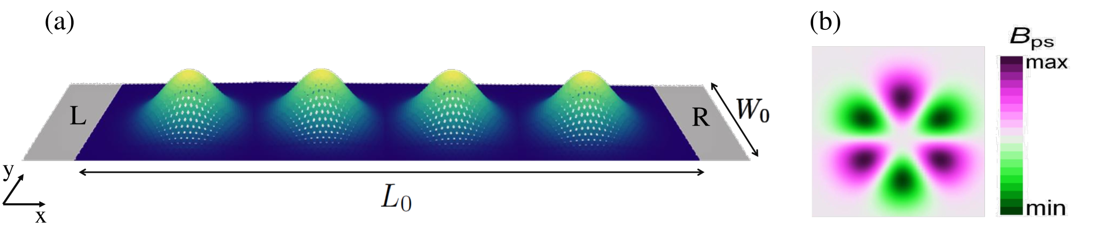
Figure 1: (a) Schematic representation of the two-terminal system. The central part of the ribbon has dimensions $L_{0}\times W_{0}$ and the zigzag direction is along to the $x$ axis. The terminals are labeled $L$ and $R$. The system is deformed by an array of $N_{G}$ out-of-plane Gaussian deformations in series. (b) Profile of the pseudo-magnetic field for one Gaussian bump in $K$ valley.

In the Landauer–Büttiker formalism, the two terminal conductance depends on the transmission probability that one electron injected along the left edge of the scattering region or device will transmit to the right edge. Here, we consider as scattering region the central section where the out-of-plane Gaussian deformations are included (see Fig. 1(a)). It is noteworthy that to access the valley degree of freedom a mixed representation is required. We have to consider the transverse modes of the contacts as well as the modification of the hopping energies between neighboring sites in the lattice. With this in mind, we calculate the transmission probability by matching the wave functions in the scattering region to the Bloch modes of the pristine contacts Ando (1991); Khomyakov et al. (2005). The transmission matrix elements for the incoming mode $m$ in the left contact and outgoing mode $n$ in the right contact can be expressed as:

$$\begin{split}&\tau_{n,m}=\sqrt{\frac{v_{R,n}}{v_{L,m}}}\left[{u}^{\dagger}_{R,n}G_{RL}Q_{0}u_{L,m}\right]\end{split}$$ (4)

where ${u}_{R,n}$ (${u}_{L,m}$) is the outgoing $n$ (incoming $m$) mode, $v_{R,n}(v_{L,m})$ is the velocity of the mode ${u}_{R,n}$ (${u}_{L,m}$), $G_{RL}$ is the Green’s function and $Q_{0}$ is the source term. Using the mode matching method we can easily split the conductance, $G=(2e^{2}/h)\sum_{m,n}\mid\tau_{n,m}\mid^{2}$, into their valley components $G=(2e^{2}/h)\left[\gamma_{K}+\gamma_{K^{\prime}}\right]$, where the valley transmission $\gamma_{K(K^{\prime})}=\sum_{m\in K(K^{\prime}),n}\mid\tau_{n,m}\mid^{2}$ is related to the transmission probability that the incoming electron in mode $m$ in $K$ or $K^{\prime}$ valley is scattered to mode $n$ in $K(K^{\prime})$ valley . Once the transmission per valley is calculated the polarization is easily determined by:

$$\begin{split}P_{K(K^{{}^{\prime}})}=\frac{\gamma_{K(K^{\prime})}}{(\gamma_{K}+\gamma_{K^{{}^{\prime}}})}\end{split}$$ (5)

II.1 Single Gaussian deformation

The transport properties of a single graphene nanobubble have been previously investigatedSettnes et al. (2016); Carrillo-Bastos et al. (2018); Stegmann and Szpak (2018); Milovanović and Peeters (2018); Carrillo-Bastos et al. (2014), in this section for completeness reasons we start presenting the main results for conductance and valley polarization, then, we use the wave function matching technique to gain physical insight into the origin of the observed valley effect. We consider a scattering region with dimensions $L_{0}\approx 12.8$ nm and $W_{0}\approx 14.8$ nm with a Gaussian bump of fixed-parameter $b=22a_{c}=3.12~{}\text{nm}$ localized exactly at the center of the system. The conductance calculation requires the transmission probability $\tau_{n,m}$ between transverse modes, we therefore identify in Fig. 2(a)-(b) the low energy transverse mode dispersion around $K$ and $K^{\prime}$ valley in the contacts (we use the primitive unit cell with $a_{z}=\sqrt{3}a_{c}$). Fig. 2(c) shows the evolution of the conductance for different values of the parameter $\alpha=(A/b)^{2}$, which determines the strain generated by the bubble. For bubbles with low curvature, the conductance presents sharp dips at the outset of a new conductance plateau, larger curvatures (increase in the value of $A$) widen the dips and degrade the overall conductance. From the point of view of valley transport, it has been observed (see Fig. 2(d)) that a single Gaussian deformation induces some degree of valley polarization for the lower energy transverse modes, obviously the fully valley polarized zigzag edge state plateau ($P_{K^{\prime}}=1$) is disregarded.

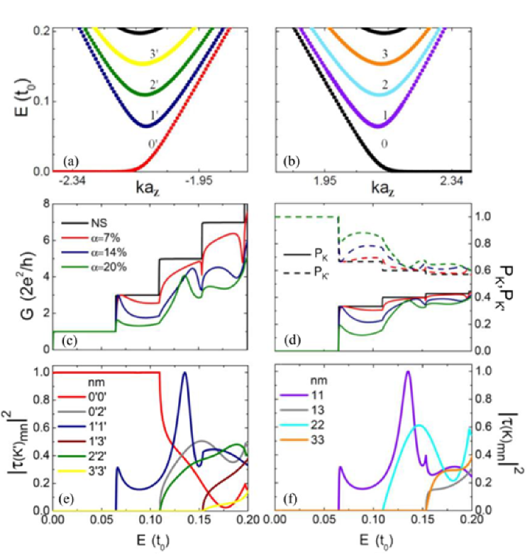
Figure 2: Band structure for a zigzag graphene nanoribbon of width $W_{0}\approx 14.8$ nm around (a) $K^{\prime}$ valley and (b) $K$ valley. (c) Conductance and (d) Valley polarization $P_{K^{\prime}}$ and $P_{K}$ in the presence of one out-of-plane Gaussian deformation for different values of the strain parameter $\alpha$. Transmission probability for the low energy modes in (d) $K^{\prime}$ valley and (e) $K$ valley produced by one Gaussian bump with $\alpha=20\%$.

It is worth stressing that the electric current in the contacts is carried by independent transverse modes, so the observed valley imbalance introduced by the Gaussian deformation is, in the end, a mode mixing effect. We can have a clear picture of the intervalley and intravalley scattering processes using eq. (4), this is done for the deformation with $\alpha=20\%$ in Fig. 2(e)-(f) where $|\tau_{n,m}|^{2}$ is plotted for the low energy modes in $K^{\prime}$ and $K$ valley respectively. The transmission probabilities reveal that the valley filter effect is entirely created by the fully valley polarized zigzag edge state mode, $|\tau_{0^{\prime},0^{\prime}}|^{2}=1$ until the onset of the second transverse mode at $E_{2^{\prime}(2)}=0.11t_{0}$. In general, there is no such a thing as electrons in one valley are transmitted through the deformation while electrons in the other valley are reflectedChaves et al. (2010), transverse modes in $K^{\prime}$ valley are scattered in a similar way as transverse modes in the opposite $K$ valley. The valley filter effect is purely and simply observed because $K^{\prime}$ valley has an extra mode.

It is also interesting to look at the peak $|\tau_{1^{\prime},1^{\prime}(1,1)}|^{2}=1$ at $E=0.135t_{0}$ and the dip in $|\tau_{0^{\prime},0^{\prime}}|^{2}=0$ at $E=0.177t_{0}$, both energies signal the presence of quasi-bound statesCarrillo-Bastos et al. (2014) below the third ($E_{3^{\prime}(3)}=0.154t_{0}$) and fourth ($E_{4^{\prime}(4)}=0.197t_{0}$) transverse modes. We find that the energy of these new states ($E_{4}-0.177t_{0}=0.02t_{0}$ and $E_{3}-0.135t_{0}=0.02t_{0}$) decreases as $\alpha^{2.43}$. Although the existence of the quasi-bound state is not noticed in the conductance plot, different lineshapes for transmission probabilities of independent modes and the suppression of intravalley scattering for others ($|\tau_{0^{\prime},1^{\prime}}|^{2}=|\tau_{1^{\prime},2^{\prime}(1,2)}|^{2}=|\tau_{2^{\prime},3^{\prime}(2,3)}|^{2}=0$) show that the Gaussian deformation scatters differently electrons on transverse modes in the same valley. The observed features are not absolutely governed by the pseudo-magnetic field ($B_{ps}\approx 515~{}\text{T}$ for $\alpha=20\%$) or the geometry of the scatterer, note that there are signatures on the conductance or transmission for energies below $E_{ps}=\hbar v_{F}/\ell_{B}\approx 0.19t_{0}$ and $E_{\text{scatt}}=\hbar v_{F}\pi/b\approx 0.2t_{0}$.

In short, we have shown that for one out-of-plane Gaussian deformation the valley imbalance is entirely created by the zigzag edge states mode, unfortunately, this fact seriously restricts its use as valley filter device. On the other hand, we also highlight the multimode nature of the electronic transport, although at first glance this may seem undesirable, in periodic structures mode mixing results in the formation of mini-stopbands Leng and Lent (1993); Benisty (2009). These local gaps in the band structure reject specific transverse modes; in the next section using a sequence of out-of-plane Gaussian deformations, we explore this notch filter effect in the valley transport domain.

II.2 Strain Superlattice: 1D Gaussian Chain.

We arrange $N_{G}$ Gaussian bumps along the $x$ direction, the centers of the bumps are separated by $d=52\sqrt{3}a_{c}\approx 12.79~{}\text{nm}$, the width of the bumps $b=22a_{c}=3.12~{}\text{nm}$ and the width of the zigzag nanoribbon $W_{0}\approx 14.8$ nm are the same as the previous section. The center of the first(last) Gaussian is located at $d/2$ from the left(right) contact, so the length of the central region is $L_{0}=N_{G}d$. To promote strong mode coupling and subsequently the formation of mini-stopbands from the very beginning we start with a large number of Gaussians ($N_{G}=15$); in Fig. 3(a) we follow the evolution of the conductance of this 1D Gaussian chain for different values of $\alpha$. The conductance shows strong modulation indicating the formation of well-defined minibands, however, looking at the transport signatures it is clear that there are two distinct features. The first kind produces rapidly oscillating conductance peaks, illustrating mode mixing, the number of peaks in one band is equal to the number of Gaussian deformations $N_{G}$. We do not show but LDOS plots of the peaks in these bands present high electronic density precisely on the Gaussian deformation region, therefore, these bands are originated by the coupling of the quasi-bound states localized on individual bubbles. Highly localized states are weakly coupled and result in narrow bands for $\alpha=20\%$, while less localized wave functions are strongly coupled and produce wide bands for $\alpha=7\%$. On the other hand, the second element in the conductance produces perfectly quantized conductance plateaus ($G=G_{0}=2e^{2}/h$), as the value of $\alpha$ increases, so do the number and the width of them. These plateaus are fully valley polarized in $K^{\prime}$ valley as shown in Fig. 3(b)-(d); notably, the combination of strain, periodicity and mode mixing produces a highly efficient valley filter.

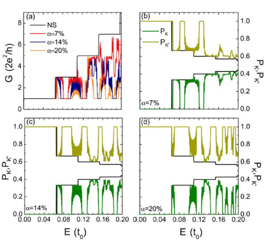
Figure 3: (a) Conductance for a zigzag graphene nanoribbon with an arrangement of $N_{G}=15$ Gaussian deformations and $W_{0}\approx 14.8$ nm. Valley polarization $P_{K^{\prime}}$ and $P_{K}$ for the same system with (b) $\alpha=7\%$, (c) $\alpha=14\%$ and (d) $\alpha=20\%$

Although both types of Conductance signatures (resonant peaks and plateaus) show integer values of $G_{0}$, the transmission probabilities of individuals modes are not totally quantized, the quantization is the result of intra-valley mode mixing. Just like in the single Gaussian deformation exposition $|\tau_{0^{\prime},0^{\prime}}|^{2}=1$ for $E\leq E_{2^{\prime}(2)}=0.11t_{0}$, in this way, the first two plateaus $P_{K^{\prime}}=1$ seen in Fig. 3(b)-(d) are produced by the zigzag edge states traverse mode. While higher energy valley polarized plateaus are created by incoming electrons in mode $m=0^{\prime}~{}\text{and}~{}2^{\prime}$ scattered into mode $n=2^{\prime}$ of the $K^{\prime}$ valley, in all of the cases studied we found $|\tau_{2^{\prime},2^{\prime}}|^{2}>0.4$. This is another strength of the 1D Gaussian superlattice valley filter because higher energy transverse modes are less affected by edge roughness.

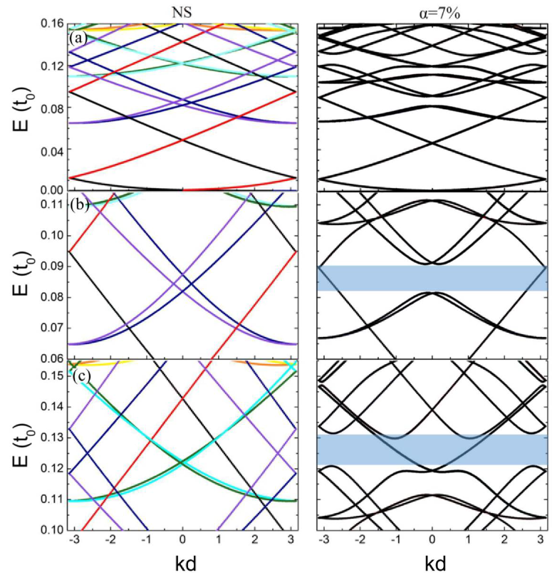
Figure 4: Left panel: folded band structure of a zigzag graphene nanoribbon without deformation and supercell lattice constant $d=52a_{z}$ and $W_{0}\approx 14.8$ nm, the colours identify the transverse modes of the primitive unit cell presented in Fig. 2(a)-(b) . Right panel: band structure of an infinite 1D chain of out-of-plane Gaussian deformations with $\alpha=7\%$. Close-up at the energy region corresponding to the second (b) and third valley (c) filter plateau $P_{K^{\prime}}=1$ and $P_{K}=0$ in Fig. 3(b).

In order to further characterize the valley filter effect, we calculated the band structure of the corresponding infinite 1D chain of Gaussian bumps with $\alpha=7\%$. The result is presented in the right panel of Fig. 4, a close-up at the energy region of the second and third valley filter plateau is shown in panels (b) and (c), the shaded regions mark the exact location and width of the plateaus. We also plot as a reference in the left panels the folded band structure of the same nanoribbon without out-of-plane deformations, the colors correspond to the independent transverse modes of the primitive unit cell of Fig. 2(a)-(b). Due to the folding, the unstrained supercell shows crossings between modes in the same or in the opposite valley, it is important to note that the periodic potential could lift the degeneracy at these points Benisty (2009). A comparison between the left and right panels of Fig. 4 suggests that mini-stopbands (anticrossings) appear as a result of the coupling between counter-propagating modes in the same valley. In general terms, contra-directional modes $m$ and $n$ get coupled when $k_{m}-k_{n}=\Delta k_{m,n}=\pm\ell G$, where $\ell$ is an integer, $G=2\pi/d$ , $k_{m}=\sqrt{(E/\hbar v_{F})^{2}-q_{m}^{2}}$ and $q_{m}=\pi(m+\frac{1}{2})/W_{0}$. Diagonal couplings ($m=n$) generally appear at the Brillouin zone boundary ($k_{m}=\pi/d$); however, we are observing diagonal (anti)crossings at different zone values. To confirm the formation of standing waves, we calculated the energy ($E_{mm}^{\ell}$) where the Bragg condition is fulfilled for independent modes:

$$E_{mm}^{\ell}=\frac{3t_{0}a_{c}}{2}\sqrt{\left(\frac{\ell\pi}{d}\right)^{2}+\left(\frac{\pi(m+\frac{1}{2})}{W_{0}}\right)^{2}}$$ (6)

It is clearly seen in the left panel of Fig. 4(b)-(c) crossings at $E_{1^{\prime}1^{\prime}(11)}^{1}=0.085t_{0}$ and $E_{1^{\prime}1^{\prime}(11)}^{2}=0.124t_{0}$ for the blue(purple) band and anticrossings in the right panel around the same energies. Further, the mini-stopband opened by the Bragg reflection of modes $m=1^{\prime},1$ is the physical effect behind the formation of the second valley filter plateau, this is concurrent with the mode transmission probability $|\tau_{0^{\prime},0^{\prime}}|^{2}=1$ calculated in the previous section. The third valley filter plateau is also originated by the coupling of counter-propagating modes, however, in this case there are diagonal ($m=1^{\prime}(1),2^{\prime}(2)$) and off-diagonal ($m=0^{\prime}(0)$ and $n=2^{\prime}(2)$) couplings involved. Based on the previous analysis one may think that periodicity alone promotes valley filter. However, this is not the case, the increase in the value of $\alpha$ strengthens the couplings between the low energy modes enlarging the anticrossings, and therefore the width of the firsts valley filter plateaus. It also fosters the mixing of higher energy modes producing additional plateaus.

To quantify the valley filter capability of the 1D Gaussian superlattice, we define

$$\begin{split}Q_{K^{{}^{\prime}}}=\left[\frac{E(P_{K^{{}^{\prime}}}>0.98)-E_{\text{edge}}}{E_{T}}\right]\times 100,\end{split}$$ (7)

where $E(P_{K^{{}^{\prime}}}>0.98)$ are the energy points with valley polarization $P_{K^{{}^{\prime}}}>0.98$, $E_{\text{edge}}$ is the energy of the fully valley polarized zigzag edge states ($E_{\text{edge}}=q_{1}\frac{3a_{c}}{2}t_{0}=\left[\frac{3\pi}{2W_{0}}\right]\frac{3a_{c}}{2}t_{0}$) and $E_{T}$ is the energy bandwidth (in our case $E_{T}=0.2t_{0}$). For the supperlattices presented in Fig. 3 we obtain $Q_{K^{{}^{\prime}}}=9.1\%$ for $\alpha=7\%$, $Q_{K^{{}^{\prime}}}=22.5\%$ for $\alpha=14\%$ and $Q_{K^{{}^{\prime}}}=33.3\%$ for $\alpha=20\%$. These numbers confirm that the Gaussian out-of-plane superlattice offers significant advantages over the single deformation. First, The valley filter effect does not require a fine tuning of the energy since the filter appears at different and wider energy regions. Second, the superlattice demands low values of strain ($\alpha$). Third, the superlattice does not depend on perfect zigzag edges given that low energy transverse modes get coupled and generate valley filters. $Q_{K^{{}^{\prime}}}$ allows, not only to quantify the effectiveness of the filter but also the impact of the superlattice parameters on its performance. To that end, we modify, one at a time, the values of the height ($A$), the width ($b$) and the distance ($d$) for the superlattice presented in Fig. 3(c) ($A=1.17~{}\text{nm}$, $b=3.12~{}\text{nm}$, $d=12.79~{}\text{nm}$ and and $N_{G}=15$). The results are summarised in table 1, where $Q_{K^{{}^{\prime}}}^{u}$ is the valley filter capability when the value of $u=A,b,d$ is reduced/increased ($\downarrow/\uparrow)$ by 10, 20 and 30%. In order to understand the behaviour of $Q_{K^{{}^{\prime}}}^{u}$, note that the values of $A$ and $b$ are related with the strength and the extend of the PMF ($|B_{ps}|\propto\alpha$). A contraction of 10, 20 and 30% in $A$, in fact, is a reduction of 19, 36 and 51% in the strength of the PMF. The weakening of the PMF produces a less effective coupling between counter-propagating modes compressing the value of $Q_{K^{{}^{\prime}}}^{A}$. For $b$, although the region with the PMF is shrunk, the process is reversed and the strength of the PMF is risen by 23, 56 and 100%. Thus, $Q_{K^{{}^{\prime}}}^{b}$ first rises when the electrons flowing from the left to the right contact sense a higher PMF, then declines when the PMF region is too narrow than only few electrons are filtered. Notwithstanding the reductions of $Q_{K^{{}^{\prime}}}$ observed in table 1, the 1D Gaussian superlattice continues to be a more effective valley filter than the single Gaussian bubble for similar $A$ and $b$ parameters Milovanović and Peeters (2016, 2016). Regarding the inter Gaussian deformation distance, we observed that in general, larger $d$ weakens the cascaded configuration of the filter. However, oscillations in $Q_{K^{{}^{\prime}}}^{d}$ can be seen given that additional transverse modes can get coupled.

Variation (%)	$Q_{K^{{}^{\prime}}}^{A}$ ($\downarrow$)	$Q_{K^{{}^{\prime}}}^{b}$ ($\downarrow$)	$Q_{K^{{}^{\prime}}}^{d}$ ($\uparrow$)
0	22.5	22.5	22.5
10	14.4	24.2	20.5
20	11.2	23.6	17.0
30	8.9	20.3	17.2

Table 1: Valley filter capability $Q_{K^{{}^{\prime}}}^{u}$ when the value of $u=A,b,d$ is reduced/increased ($\downarrow/\uparrow)$ by 10, 20 and 30%. The unperturbed (0%) parameters corresponds to the superlattice shown in Fig. 3(c) $\alpha=14\%$ ($A=1.17~{}\text{nm}$, $b=3.12~{}\text{nm}$, $d=12.79~{}\text{nm}$ and $N_{G}=15$).

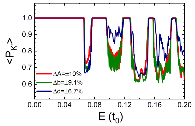
Figure 5: Average Valley polarization $<P_{K^{\prime}}>$ for the 1D Gaussian supperlattice presented in Fig. 3(c) $\alpha=14\%$ ($A=1.17~{}\text{nm}$, $b=3.12~{}\text{nm}$, $d=12.79~{}\text{nm}$ and $N_{G}=15$) with $A$ (height) disorder (red line), $b$ (width) disorder (green line) and $d$ (distance) disorder (blue line). The calculated valley filter capabilities for the disordered systems are: $Q_{K^{{}^{\prime}}}^{A}=21.7\%$, $Q_{K^{{}^{\prime}}}^{b}=22.7\%$ and $Q_{K^{{}^{\prime}}}^{d}=20.7\%$.

Another important point to tackle is the robustness of the valley filter against periodicity perturbations. We consider the effect of disorder in $A$, $b$ and $d$ by modifying, for each one of the Gaussians in the superlattice, the value of $u=A,b,d$ according to $u=u_{0}+\delta u$. Again, the unperturbed values ($u_{0}$) are the parameters of the 1D Gaussian chain with $\alpha=14\%$ ($A_{0}=1.17~{}\text{nm}$, $b_{0}=3.12~{}\text{nm}$, $d_{0}=12.79~{}\text{nm}$ and $N_{G}=15$) and $\delta u$ is a random number uniformly distributed between $[-\Delta u,\Delta u]$. Specifically, we fixed $\Delta A=0.1A_{0}$, $\Delta b=0.091b_{0}$ and $\Delta d=0.067d_{0}$; the values of $\Delta b$ and $\Delta d$ were chosen to avoid overlapping and deformations none wider than the width of the nanoribbon ($W_{0}$). The valley polarization averaged over 20 disorder realisations for $A$ (red line), $b$ (green line) and $d$ (blue line) is shown in Fig. 5. It can be seen that the valley filter effect is slightly modified by disorder. Besides that, the valley filter capabilities of the disordered superlattices $Q_{K^{{}^{\prime}}}^{A}=21.7\%$, $Q_{K^{{}^{\prime}}}^{b}=22.7\%$ and $Q_{K^{{}^{\prime}}}^{d}=20.7\%$ follow the same trends and have the same physical explanation of the valley filter capabilities of the pristine superlattices calculated and discussed in the previous paragraph.

III Modeling Valley Transport using Artificial Neural Networks

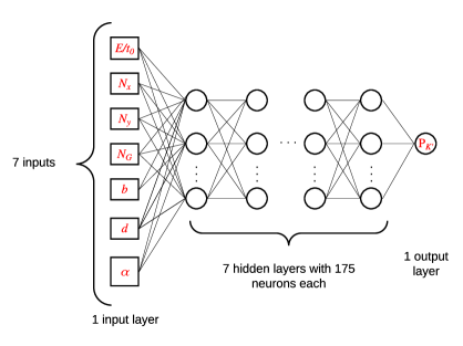
Figure 6: Feedforward fully connected deep neural network architecture used for predicting valley polarization. The network consists of: an input layer with seven neurons; seven hidden layers with one hundred seventy five neurons each and one output layer with a single neuron. The neurons have hyperbolic tangent activation with exception of output layer neuron that has linear activation.

To take advantage of the enhanced valley filter effect produced by the Gaussian deformations, it desirable to know in advance the number, energy and width of the valley filter plateaus for a given supperlattice. In this section we deal with this problem using Artificial Neural Networks (ANNs). ANNs are computational modeling tools that have found extensive acceptance in many disciplines for modeling complex real-word problems Haykin (1994); Aggarwal (2018). The layered architecture of ANN (input, hidden and output) is comprised of densely interconnected adaptive simple processing elements called artificial neurons, when a network has more than two/three hidden layers it is also called deep neural network (DNN) Basheer and Hajmeer (2000). The neurons are connected by synaptic weights, during the training process the weights are incrementally adjusted and thus the network can efficiently learn to perform a specific task. In supervised learning, the network is provided with a correct answer (output) for every input pattern from the training dataset, Error-Correction Learning (ECL) rule is employed to gradually reduce the overall network error. This means that the arithmetic difference (error) between the ANN solution at each stage (cycle) during training and the corresponding answer is used to modify the synaptic weights. The training of ANN occurs from input patterns of the training dataset in an interactive process: (i) A sample of this training dataset is randomly chosen and introduced in the input layer. (ii) The sample is propagated to the output layer in a linear combination of data and weight vectors. (iii) The difference between the output of the neural network and the dataset is used to adjust the weight vector. The back-propagation is responsible for propagating the error which can be considered as the loss function to be minimized. The weights values are then updated according to the gradient descent in a way that the total loss is reduced, and a better model is obtained. These steps are repeated until the network reaches either a minimum error or a finite number of iterations. To assess the performance of a trained model, it is common to use the coefficient-of-determination, $R^{2}$, representing the agreement between the predicted and target outputs. Other more involved methods for monitoring network training and generalization are based on information theory Swingler (1996).

One advantage of using DNNs to model valley polarization is their ability to incorporate all the operating parameters in one model; we assume that valley polarization may be expressed as unknown function $P_{K^{\prime}}=f(E/t_{0},N_{x},N_{y},N_{G},b,d,\alpha)$ of the number of atoms in the $x$ axis direction $N_{x}$, the number of atoms in the $y$ axis direction and the previously defined variables $E/t_{0}$, $N_{G}$, $b$, $d$, and $\alpha$; in this way, the input and output layers are defined from prior knowledge of the problem (see Fig. 6). It is important to highlight that some of the inputs are highly correlated, but even though we decide to include them because they are design parameters of the superlattice, on the other hand, highly correlated inputs do not present any threat to the training and validation process of the DNN. To determine the ideal number of the hidden layers is one of the most critical tasks; several rules are available in the literature including those that relate the hidden layer size to the number of neurons in input and output layers Boger and Guterman (1997); Berry and Linoff (2004). However, the high non-linearity of the problem forces us to vary the number of hidden layers and their neurons using the training error as a decision criterion. The final DNN architecture has seven hidden layers with one hundred seventy-five neurons each as shown in Fig. 6.

III.1 Training and validation

Parameter	Avg.	Std.	Min.	Max.
$N_{x}$	1257.76	769.01	40.00	3601.00
$N_{y}$	73.81	20.95	20.00	150.00
$N_{G}$	12.14	8.62	0.00	60.00
$b$	2.97	0.77	0.00	4.54
$\alpha$	0.16	0.12	0.00	0.40
$d$	11.16	3.29	0.00	22.13

Table 2: Statistical dataset summary of the superlattice design parameters including the average, standard deviation and minimal/maximal for each variable.

The dataset used in this experiment was generated by the wave function matching technique and the Green’s Function for 117 distinct configurations of the 1D Gaussian supperlattice. Individual configurations defined by the 6-tuple $(N_{x},N_{y},N_{G},b,d,\alpha)$ were labeled with the calculated $P_{K^{\prime}}$ for each one of the 500 energy points ($E/t_{0}\in[{0.001,0.5}]$). The dataset summary presented in table 2 helps not only to analyse the statistical distribution of the configuration space involved in the ANN training, but it also helps understanding how this problem could be modeled, in this case, as supervised regression. Training an ANN is typically conducted separating the dataset into two sets: training and testing. In this way, one trains the model on the training data and then evaluates the performance of the model on the testing dataset. It is important that the two sets are non-intersecting (i.e. no test input pattern appear in the training dataset) so that a fair evaluation of the model generalization is obtained. We randomly split the 58500 ($117\times 500$) data samples into 80% for training and 20% for testing; in addition, 20% of training dataset was used for hyperparameter tunning (i.e changing the number of neurons or layers). Training of the model has carried out with a custom TensorFlow Abadi et al. (2016) implementation. The input and output data were preprocessed by z-normalization into vectors whose mean is approximately 0 while the standard deviation is in a range close to 1 to satisfy the transfer function and to make the training fasterHaykin (1994); Aggarwal (2018). During training, the loss function is monitored and terminated when convergence is obtained. In Fig. 7 we plot the number of epochs vs MSE (Mean Squared Error) for training and validation datasets. As the number of epochs increases, the MSE is reduced because the weights are updated after each iteration. The loss is too high on early epochs, so the model is still underfitting both the training and the validation set. Ordinarily, a neural network learns in stages, moving from the generalization of simple to more complex mapping functions as the training session progresses. This is exemplified by the typical situation in which the MSE decreases with an increasing number of epochs during training: it starts off at large values, decreases rapidly, and then continues to decrease slowly as the network makes its way to a local minimum on the error surface. We identified the onset of overfitting through the use of cross-validation, for which the training data are split into an estimation subset and a validation subset. The estimation subset is used to train the network as usual, but the training session is stopped periodically, every so many epoch, and the network is tested on the validation subset after each period of training. This simple, effective, and widely used approach to training neural networks is called early stopping Thodberg (1996). The training was stopped at epoch 385, at this stage we are sure that the DNN is able to learn from the training set just enough to be able to generalize with the validation set ensuring good performance on unseen data such as the testing set. Otherwise, overtraining, which refers to exceeding the optimal time of ANN training, could result in worse predictive ability of the network. As both training and validation loss decrease at a similar rate, the best model weights could be found when validation loss stopped improving. From epoch 385, the model would stop generalizing and start learning the statistical noise in the training dataset. The results using DNN for the prediction showed accuracy measures in: $R^{2}$ (test data) = $0.970$ and MSE (test data) = $0.001$.

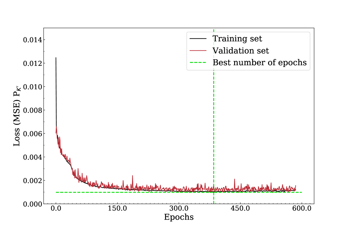
Figure 7: Variation of the MSE versus number of epochs for training and test data.

As shown previously, when we do a single evaluation on our test set we get only one outcome; this may be the result of some unknown bias. With this in mind, we decided to leverage another important cross-validation technique; k-fold assess how the results of statistical analysis and/or the machine learning model generalize independent data sets. To take advantage of this technique, the training dataset was partitioned into ten equal-sized subsamples. A single subsample was retained as the validation data for testing the model, and the remaining nine subsamples were used to train the model. The cross-validation was repeated ten times, with each of the ten subsamples used exactly once as the validation data. In order to preserve the target variable ($P_{K^{\prime}}$) distribution in training and validation sets, the continuous target variable was represented as a categorical variable. To do so, ten buckets/bins $[{0.5,0.55}]$, $[{0.56,0.61}]$,…,$[{0.94,1}]$ were defined according to the value of $P_{K^{\prime}}$. The ten rounds performance metrics, as shown in the table 3, were collected and averaged to produce a single estimation. Each round also shows the performance metrics for the trained model predictions on the testing dataset. As mentioned previously, when we create ten different models and test it on ten different validation sets. By training ten different models we can understand better what’s going on. The best scenario is that the DNN accuracy is high and the error is low and similar in all ten splits. This means that our model and our data are consistent and we can be confident that by training it on all the data set and using it in other real-world scenarios will lead to similar performance.

#	T. MSE	T. R2	V. MSE	V. R2	TS. MSE	TS. R2
1	0.002	0.926	0.026	0.917	0.001	0.959
2	0.002	0.925	0.031	0.910	0.002	0.946
3	0.002	0.926	0.031	0.909	0.002	0.947
4	0.002	0.926	0.026	0.922	0.002	0.952
5	0.002	0.925	0.025	0.921	0.002	0.945
6	0.002	0.921	0.025	0.928	0.002	0.950
7	0.002	0.926	0.027	0.917	0.001	0.959
8	0.002	0.925	0.027	0.915	0.002	0.954
9	0.002	0.924	0.026	0.920	0.002	0.951
10	0.002	0.924	0.027	0.913	0.001	0.955
AVG	0.002	0.925	0.027	0.917	0.002	0.952

Table 3: Performance metrics for training (T.), validation (V.) and test (TS.) dataset per round of K-fold cross validation.

III.2 Optimal 1D Gaussian Chain

In the previous paragraph using data-analysis tools, we show that the DNN is able to learn the relationship between the design parameters of the 1D Gaussian chain and valley polarization. For a physics-related demonstration of the performance of the DNN on unseen scenarios, $P_{K^{\prime}}$ is calculated as function of $N_{G}$ for $N_{y}=70~{}(W_{0}\approx 14.8~{}\text{nm})$ , $b=3.12~{}\text{nm}$ and $\alpha=7\%~{}\text{and}~{}14\%$; the results are plotted in Fig. 8. First, we observe the DNN learned that the zigzag edge states plateau is always present, irrespective of the values of $N_{G}$ and $\alpha$. Second, a comparison between Fig. 8a and Fig. 4 or Fig. 3b for $\alpha=7\%$, and, a comparison between Fig. 8b and Fig. 3c for $\alpha=14\%$ clearly show that the DNN predicted the energy position of the valley plateaus as function of $N_{G}$ and $\alpha$. In addittion, Fig. 8 makes explicit that few Gaussian deformations mimic the effect of an infinite deformation chain; in section IIB using the Green’s functions we mentioned that could be the case, but now with the DNN this becomes evident with much less computational effort.

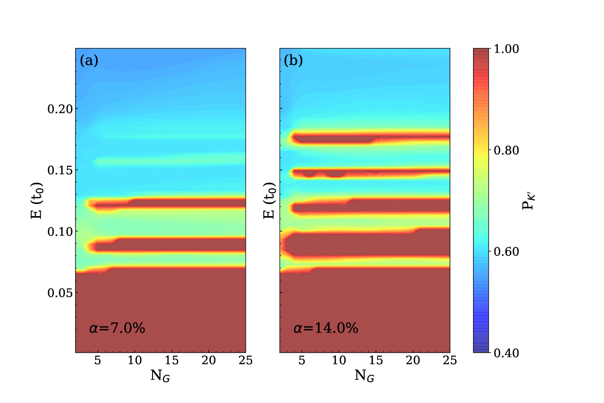
Figure 8: Predicted valley polarization $P_{K}^{\prime}$ as function of E(t₀) and number of gaussians N_G for (a) $\alpha=7\%$ and (b) $\alpha=14\%$. The dataset was generated with $N_{y}=70~{}(W_{0}=14.8~{}\text{nm})$, $b=3.12~{}\text{nm}$ and $d=12.7~{}\text{nm}$

The DNN reproduces the electronic valley transport properties of the 1D Gaussian superlattice with an accuracy close to the Green’s functions technique. This new tool can be used to quickly visualize the relationships among the strain superlattice design variables ($N_{x},N_{y},N_{G},b,d~{}\text{and}~{}\alpha$) and their effect on valley transport. One example is shown in Fig. 9a where the valley filter capability $Q_{K^{{}^{\prime}}}$ is calculated as function of $N_{G}$ for $\alpha=7,14~{}\text{and}~{}20\%$. Once more it is seen that a small number of Gaussian deformations in a series configuration enhance valley filter capabilities. However, we noticed that $Q_{K^{{}^{\prime}}}$ predicted by DNN are smaller than the true values calculated by the Green’s functions. The DNN accurately predicts the energy location of the valley plate but fails to estimate its width. We can also use the trained DNN as a superlattice design tool by searching for the 1D Gaussian superlattice with the largest $Q_{K^{{}^{\prime}}}$ and the smallest strain ($\alpha$) and number of Gaussians ($N_{G}$). To restrict the number of degrees of freedom in the problem but without loss of generality we fix the width of the nanoribbon $N_{y}=70~{}(W_{0}=14.8~{}\text{nm})$, $b=3.12~{}\text{nm}$ and $d=12.7~{}\text{nm}$. The DNN calculated $P_{K^{\prime}}$ for 696 distinct values of $\alpha\in[{0.01,0.3}[$ and $N_{G}\in[{2,26}[$, then the generated dataset was sorted by $Q_{K^{{}^{\prime}}}$ in descending oder. According to our criterion, the optimal superlattice corresponds to the system with parameters $N_{G}=6$ and $\alpha=15\%$. In Fig. 9b we present $P_{K^{\prime}}$ calculated by the DNN and the Green’s function for the optimal case, it is observed that the DNN predicts the valley filter for all the energy position and width of the valley plateaus with acceptable accuracy. Given that our main objective is the study of the valley filter effect we trained the DNN as a model that approximates $P_{K^{\prime}}\sim 1$ as good as possible, by virtue of this choice the DNN does not reproduce the valley polarization oscillations for $P_{K^{\prime}}<0.8$. Finally, we want to stress that the optimal configuration meets our searching criteria, but other criteria can be established. For example, one can search for the valley filter with the largest number of Gaussians and the smallest strain. The important point is that DNN accurately and rapidly calculates $P_{K^{\prime}}$ and can be used as a design tool for highly efficient valley filters.

Figure 9: (a) $Q_{K^{{}^{\prime}}}$ as a function of $N_{G}$ for different values of $\alpha$ calculated by the DNN. (b) Valley polarization calculated by the Green’s function (GF) and the DNN for the optimal graphene superlattice parameters $N_{G}=6$, $\alpha=15\%$, $N_{y}=70~{}(W_{0}=14.8~{}\text{nm})$, $b=3.12~{}\text{nm}$ and $d=12.7~{}\text{nm}$.

IV Outlook and Conclusions

The manipulation of the valley quantum number requires first effective ways to polarise the current, second, valley low loss transmission systems, and finally valley detection mechanisms. The proposed 1D Gaussian strain superlattice in a narrow channel of a Field-Effect Transistor can be used to inject or to detect valley polarized currents in a broad range of gate voltages. The key ingredient is a superlattice with a period smaller than the electron mean free path to induce the folding of the bands and the coupling of counter-propagating modes. To achieve this, graphene can be deposited on nanopatterned substratesJiang et al. (2017); Gill et al. (2015); Hinnefeld et al. (2018); Banerjee et al. (2019); Zhang et al. (2018); local measurements of the electronic properties have confirmed the appearance of pseudo-Landau levels in the strained regions providing direct evidence of the formation of strain superlatticesJiang et al. (2017). Concretely, two approaches can be used to produce the studied 1D superlattice. (i) Recent works have transferred graphene to substrates with distinct arrays of nanopillarsJiang et al. (2017); Xu et al. (2018), the strain profile of graphene on a single pillar yields a six-fold symmetry pseudo-magnetic field similar to the one generated by one Gaussian out-of-plane deformationNeek-Amal et al. (2012). (ii) Control of the voltage on atomic force microscopy (AFM) tips creates graphene bubbles with a Gaussian profile at defined locationsNemes-Incze et al. (2017); Jia et al. (2019).

On the other hand, our results show that the valley polarization of the current is robust against variations of the strain superlattice parameters ($A$, $b$ and $d$), thus graphene does not need to adhere perfectly to all nanopillars, or that all graphene Gaussian bubbles obtained by the AFM tip have to have the same height and width. It is important to note that in our transport calculation we do not include the effect of wrinkles or inhomogeneous variations of the gate potential. However, we do not expect large deviations from our results when these effects are taken into account, given that graphene folds are better valley filters than a single Gaussian deformation Zhai and Sandler (2018) and the small height variations of the bubbles Zhang et al. (2018).

In summary, we presented a combined Green’s functions and Machine learning approach to study the valley filter effect in a 1D Gaussian strain superlattice. In the first part of this work, using the Green’s function and the wave function matching technique, we showed that Gaussian superlattice offers superior valley filter capabilities compared with the ones observed with a single Gaussian out-of-plane deformation. Plotting the band structure of the superlattice and identifying the transverse modes, we found that the valley filter appears as the result of the coupling between counter-propagating modes in the same valley while the strength of the scatterer (value of the pseudo-magnetic field) determines the width of the plateau. Although the Green’s function is solved recursively, the computational complexity of inverting a matrix is $\mathcal{O}(N_{y}^{\gamma})$ where $2.3\leq\gamma\leq 3$ depending on the used algorithm, this fact allows us to explore only a few points in the 6-dimensional configuration space of the design parameters ($L_{0},W_{0},N_{G},b,d~{}\text{and}~{}\alpha$) of the superlattice. With this in mind, in the last section we trained a DNN to reproduce $P_{K^{\prime}}\sim 1$; our results show that DNN can be used to predict electronic transport properties with an accuracy close to the Green’s functions technique but with much less computational effort and processing time.

.

V Acknowledgments

VT acknowledges FAPESP under grant 2017/12747-4 and FAPERJ 202.322/2018. PS received partial support from Coordenação de Aperfeiçoamento de Pessoal de Nível Superior - Brasil (CAPES) - Finance Code 001. EATS and DAB acknowledge support from FAPESP (process nos. 2012/50259-8, 2015/11779-4 and 2018/07276-5), the Brazilian Nanocarbon Institute of Science and Technology (INCT/Nanocarbono), CNPq and Mackpesquisa.

References

- Schaibley et al. (2016) J. R. Schaibley, H. Yu, G. Clark, P. Rivera, J. S. Ross, K. L. Seyler, W. Yao, and X. Xu, Valleytronics in 2D materials, Nature Reviews Materials 1, 16055 (2016).
- Sham et al. (1978) L. J. Sham, S. J. Allen, A. Kamgar, and D. C. Tsui, Valley-valley splitting in inversion layers on a high-index surface of silicon, Phys. Rev. Lett. 40, 472 (1978).
- Thompson et al. (2004) S. E. Thompson, M. Armstrong, C. Auth, M. Alavi, M. Buehler, R. Chau, S. Cea, T. Ghani, G. Glass, T. Hoffman, C. H. Jan, C. Kenyon, J. Klaus, K. Kuhn, Z. Ma, et al., A 90-nm logic technology featuring strained-silicon, IEEE Transactions on Electron Devices 51, 1790 (2004).
- Gunawan et al. (2006) O. Gunawan, B. Habib, E. P. De Poortere, and M. Shayegan, Quantized conductance in an AlAs two-dimensional electron system quantum point contact, Phys. Rev. B 74, 155436 (2006).
- Yao et al. (2008) W. Yao, D. Xiao, and Q. Niu, Valley-dependent optoelectronics from inversion symmetry breaking, Phys. Rev. B 77, 235406 (2008).
- Cao et al. (2012) T. Cao, G. Wang, W. Han, H. Ye, C. Zhu, J. Shi, Q. Niu, P. Tan, E. Wang, B. Liu, and J. Feng, Valley-selective circular dichroism of monolayer molybdenum disulphide, Nature Communications 3, 887 (2012).
- Li et al. (2014) Y. Li, J. Ludwig, T. Low, A. Chernikov, X. Cui, G. Arefe, Y. D. Kim, A. M. van der Zande, A. Rigosi, H. M. Hill, S. H. Kim, J. Hone, Z. Li, D. Smirnov, and T. F. Heinz, Valley splitting and polarization by the Zeeman effect in monolayer , Phys. Rev. Lett. 113, 266804 (2014).
- MacNeill et al. (2015) D. MacNeill, C. Heikes, K. F. Mak, Z. Anderson, A. Kormányos, V. Zólyomi, J. Park, and D. C. Ralph, Breaking of valley degeneracy by magnetic field in monolayer , Phys. Rev. Lett. 114, 037401 (2015).
- Qi et al. (2013) Z. Qi, D. A. Bahamon, V. M. Pereira, H. S. Park, D. K. Campbell, and A. H. C. Neto, Resonant tunneling in graphene pseudomagnetic quantum dots, Nano Letters 13, 2692 (2013).
- Jones et al. (2017) G. W. Jones, D. A. Bahamon, A. H. Castro Neto, and V. M. Pereira, Quantized transport, strain-induced perfectly conducting modes, and valley filtering on shape-optimized graphene corbino devices, Nano Letters 17, 5304 (2017).
- Carrillo-Bastos et al. (2016) R. Carrillo-Bastos, C. León, D. Faria, A. Latgé, E. Y. Andrei, and N. Sandler, Strained fold-assisted transport in graphene systems, Phys. Rev. B 94, 125422 (2016).
- da Costa et al. (2017) D. R. da Costa, A. Chaves, G. A. Farias, and F. M. Peeters, Valley filtering in graphene due to substrate-induced mass potential, Journal of Physics: Condensed Matter 29, 215502 (2017).
- Gorbachev et al. (2014) R. V. Gorbachev, J. C. W. Song, G. L. Yu, A. V. Kretinin, F. Withers, Y. Cao, A. Mishchenko, I. V. Grigorieva, K. S. Novoselov, L. S. Levitov, and A. K. Geim, Detecting topological currents in graphene superlattices, Science 346, 448 (2014).
- Lee et al. (2016) J. Lee, K. F. Mak, and J. Shan, Electrical control of the valley hall effect in bilayer transistors, Nature Nanotechnology 11, 421 (2016).
- Levy et al. (2010) N. Levy, S. A. Burke, K. L. Meaker, M. Panlasigui, A. Zettl, F. Guinea, A. H. C. Neto, and M. F. Crommie, Strain-induced pseudo–magnetic fields greater than 300 tesla in graphene nanobubbles, Science 329, 544 (2010).
- Settnes et al. (2016) M. Settnes, S. R. Power, M. Brandbyge, and A.-P. Jauho, Graphene nanobubbles as valley filters and beam splitters, Phys. Rev. Lett. 117, 276801 (2016).
- Carrillo-Bastos et al. (2018) R. Carrillo-Bastos, M. Ochoa, S. A. Zavala, and F. Mireles, Enhanced asymmetric valley scattering by scalar fields in nonuniform out-of-plane deformations in graphene, Phys. Rev. B 98, 165436 (2018).
- Stegmann and Szpak (2018) T. Stegmann and N. Szpak, Current splitting and valley polarization in elastically deformed graphene, 2D Materials 6, 015024 (2018).
- Milovanović and Peeters (2018) S. P. Milovanović and F. M. Peeters, Strained graphene structures: From valleytronics to pressure sensing, in Nanostructured Materials for the Detection of CBRN, edited by J. Bonča and S. Kruchinin (Springer Netherlands, Dordrecht, 2018) pp. 3–17.
- Myoung et al. (2019) N. Myoung, H. Choi, and H. C. Park, Manipulation of valley isospins in strained graphene for valleytronics, arXiv preprint arXiv:1907.09079 (2019).
- Milovanović and Peeters (2016) S. Milovanović and F. Peeters, Strain controlled valley filtering in multi-terminal graphene structures, Applied Physics Letters 109, 203108 (2016).
- Milovanović and Peeters (2016) S. P. Milovanović and F. M. Peeters, Strained graphene hall bar, Journal of Physics: Condensed Matter 29, 075601 (2016).
- Zhai and Sandler (2018) D. Zhai and N. Sandler, Local versus extended deformed graphene geometries for valley filtering, Phys. Rev. B 98, 165437 (2018).
- Park et al. (2008) C.-H. Park, L. Yang, Y.-W. Son, M. L. Cohen, and S. G. Louie, Anisotropic behaviours of massless dirac fermions in graphene under periodic potentials, Nature Physics 4, 213 (2008).
- Brey and Fertig (2009) L. Brey and H. A. Fertig, Emerging zero modes for graphene in a periodic potential, Phys. Rev. Lett. 103, 046809 (2009).
- Wang and Zhu (2010) L.-G. Wang and S.-Y. Zhu, Electronic band gaps and transport properties in graphene superlattices with one-dimensional periodic potentials of square barriers, Phys. Rev. B 81, 205444 (2010).
- Andrade et al. (2019) E. Andrade, R. Carrillo-Bastos, and G. G. Naumis, Valley engineering by strain in Kekulé-distorted graphene, Phys. Rev. B 99, 035411 (2019).
- Benisty (2009) H. Benisty, Graphene nanoribbons: Photonic crystal waveguide analogy and minigap stripes, Phys. Rev. B 79, 155409 (2009).
- Jiang et al. (2017) Y. Jiang, J. Mao, J. Duan, X. Lai, K. Watanabe, T. Taniguchi, and E. Y. Andrei, Visualizing strain-induced pseudomagnetic fields in graphene through an hBN magnifying glass, Nano Letters 17, 2839 (2017).
- Gill et al. (2015) S. T. Gill, J. H. Hinnefeld, S. Zhu, W. J. Swanson, T. Li, and N. Mason, Mechanical control of graphene on engineered pyramidal strain arrays, ACS Nano 9, 5799 (2015).
- Hinnefeld et al. (2018) J. H. Hinnefeld, S. T. Gill, and N. Mason, Graphene transport mediated by micropatterned substrates, Appl. Phys. Lett. 112, 173504 (2018).
- Banerjee et al. (2019) R. Banerjee, V.-H. Nguyen, T. Granzier-Nakajima, L. Pabbi, A. Lherbier, A. Binion, J.-C. Charlier, M. Terrones, and E. Hudson, Strain modulated superlattices in graphene, arXiv preprint arXiv:1903.10468 (2019).
- Zdeborová (2017) L. Zdeborová, New tool in the box, Nature Physics 13, 420 (2017).
- Seko et al. (2015) A. Seko, A. Togo, H. Hayashi, K. Tsuda, L. Chaput, and I. Tanaka, Prediction of low-thermal-conductivity compounds with first-principles anharmonic lattice-dynamics calculations and bayesian optimization, Phys. Rev. Lett. 115, 205901 (2015).
- Hanakata et al. (2018) P. Z. Hanakata, E. D. Cubuk, D. K. Campbell, and H. S. Park, Accelerated search and design of stretchable graphene kirigami using machine learning, Phys. Rev. Lett. 121, 255304 (2018).
- Cubuk et al. (2017) E. D. Cubuk, R. J. S. Ivancic, S. S. Schoenholz, D. J. Strickland, A. Basu, Z. S. Davidson, J. Fontaine, J. L. Hor, Y. R. Huang, Y. Jiang, N. C. Keim, K. D. Koshigan, J. A. Lefever, T. Liu, X. G. Ma, et al., Structure-property relationships from universal signatures of plasticity in disordered solids, Science 358, 1033 (2017).
- Carvalho et al. (2018) D. Carvalho, N. A. García-Martínez, J. L. Lado, and J. Fernández-Rossier, Real-space mapping of topological invariants using artificial neural networks, Phys. Rev. B 97, 115453 (2018).
- Vozmediano et al. (2010) M. A. Vozmediano, M. Katsnelson, and F. Guinea, Gauge fields in graphene, Physics Reports 496, 109 (2010).
- Ando (1991) T. Ando, Quantum point contacts in magnetic fields, Phys. Rev. B 44, 8017 (1991).
- Khomyakov et al. (2005) P. Khomyakov, G. Brocks, V. Karpan, M. Zwierzycki, and P. J. Kelly, Conductance calculations for quantum wires and interfaces: Mode matching and Green’s functions, Phys. Rev. B 72, 035450 (2005).
- Carrillo-Bastos et al. (2014) R. Carrillo-Bastos, D. Faria, A. Latgé, F. Mireles, and N. Sandler, Gaussian deformations in graphene ribbons: Flowers and confinement, Phys. Rev. B 90, 041411 (2014).
- Chaves et al. (2010) A. Chaves, L. Covaci, K. Y. Rakhimov, G. A. Farias, and F. M. Peeters, Wave-packet dynamics and valley filter in strained graphene, Phys. Rev. B 82, 205430 (2010).
- Leng and Lent (1993) M. Leng and C. S. Lent, Recovery of quantized ballistic conductance in a periodically modulated channel, Phys. Rev. Lett. 71, 137 (1993).
- Haykin (1994) S. Haykin, Neural networks: a comprehensive foundation (Prentice Hall, 1994).
- Aggarwal (2018) C. C. Aggarwal, Neural networks and deep learning (Springer, 2018).
- Basheer and Hajmeer (2000) I. A. Basheer and M. Hajmeer, Artificial neural networks: fundamentals, computing, design, and application, Journal of microbiological methods 43, 3 (2000).
- Swingler (1996) K. Swingler, Applying neural networks: a practical guide (Morgan Kaufmann, 1996).
- Boger and Guterman (1997) Z. Boger and H. Guterman, Knowledge extraction from artificial neural network models, in 1997 IEEE International Conference on Systems, Man, and Cybernetics. Computational Cybernetics and Simulation, Vol. 4 (1997) pp. 3030–3035.
- Berry and Linoff (2004) M. J. Berry and G. S. Linoff, Data mining techniques: for marketing, sales, and customer relationship management (John Wiley & Sons, 2004).
- Abadi et al. (2016) M. Abadi, P. Barham, J. Chen, Z. Chen, A. Davis, J. Dean, M. Devin, S. Ghemawat, G. Irving, M. Isard, M. Kudlur, J. Levenberg, R. Monga, S. Moore, D. G. Murray, et al., Tensorflow: A system for large-scale machine learning, in 12th USENIX Symposium on Operating Systems Design and Implementation (OSDI 16) (USENIX Association, Savannah, GA, 2016) pp. 265–283.
- Thodberg (1996) H. H. Thodberg, A review of bayesian neural networks with an application to near infrared spectroscopy, IEEE Transactions on Neural Networks 7, 56 (1996).
- Zhang et al. (2018) Y. Zhang, Y. Kim, M. J. Gilbert, and N. Mason, Electronic transport in a two-dimensional superlattice engineered via self-assembled nanostructures, npj 2D Materials and Applications 2, 31 (2018).
- Xu et al. (2018) T. Xu, A. Díaz Álvarez, W. Wei, D. Eschimese, S. Eliet, O. Lancry, E. Galopin, F. Vaurette, M. Berthe, D. Desremes, B. Wei, J. Xu, J. F. Lampin, E. Pallecchi, H. Happy, et al., Transport mechanisms in a puckered graphene-on-lattice, Nanoscale 10, 7519 (2018).
- Neek-Amal et al. (2012) M. Neek-Amal, L. Covaci, and F. M. Peeters, Nanoengineered nonuniform strain in graphene using nanopillars, Phys. Rev. B 86, 041405 (2012).
- Nemes-Incze et al. (2017) P. Nemes-Incze, G. Kukucska, J. Koltai, J. Kürti, C. Hwang, L. Tapasztó, and L. Biró, Preparing local strain patterns in graphene by atomic force microscope based indentation, Scientific Reports 7, 3035 (2017).
- Jia et al. (2019) P. Jia, W. Chen, J. Qiao, M. Zhang, X. Zheng, Z. Xue, R. Liang, C. Tian, L. He, Z. Di, and X. Wang, Programmable graphene nanobubbles with three-fold symmetric pseudo-magnetic fields, Nature Communications 10, 3127 (2019).