A general model for vegetation patterns including rhizome growth

Abstract

Vegetation patterns, a natural phenomenon observed worldwide, are typically driven by spatially distributed feedback. However, the spatial colonization mechanisms of clonal plants, driven by the growth of a rhizome, are usually not considered in prototypical models. Here we propose a general equation for the vegetation density that includes all main clonal-growth features as well as the essential ingredients leading to spatial self-organization. This generic model reproduces the phase diagram of a fully detailed model of clonal growth. The relation of each term of the model with the mechanisms of clonal growth is discussed.

I INTRODUCTION

The spatial distribution of vegetation is a key factor in ecosystems functionality as it may completely reorganize the pathways of energy and resources Meron (2015). Besides the simple homogeneous coverage, and disordered configurations, several types of inhomogeneous vegetation distributions have been reported, ranging from isolated gaps, scattered gaps arranged in a more or less regular lattice, stripes or labyrinthine patterns, patches arranged in a regular lattice, or isolated patches Meron (2015); Gowda et al. (2014). Although there are a variety of mechanisms responsible for creating and maintaining the spatial inhomogeneities, they are always associated to feedback across space Rietkerk and van de Koppel (2008); Getzin et al. (2016) from which similar patterns arise in completely different environments. Even the sequence in which the different patterns appear when changing a control parameter is often the same Gowda et al. (2014), which gives a universal character to the phenomenon of vegetation pattern formation.

Most studies of vegetation patterns consider arid environments, where water is the limiting factor. Different approaches have been considered, ranging from simple models describing vegetation only Lefever and Lejeune (1997); Lejeune and Tlidi (1999); Lejeune et al. (2002), to more sophisticated ones accounting for vegetation and water Getzin et al. (2016); Fernandez-Oto et al. (2019). Long-range competitive mechanisms are usually the reason behind pattern formation, sometimes mediated by a diffusive external agent such as water or described effectively by an interaction kernel. Thus, the selected wavelength of the pattern is the result of the interaction of two spatial scales, the range of competition, and the spatial scale given by the diffusion of vegetation.

In these models, plant competition for water is the basic factor introducing destabilizing feedback. On the other hand, vegetation propagation is usually assumed to occur by seed dispersal. However, a recent study of pattern formation in underwater meadows of seagrasses Ruiz-Reynés et al. (2017) was clearly outside the domain of applicability of these two standard hypothesis. First, although the mechanism for plant interaction was not uniquely identified, competition for water can not be a relevant interaction mechanism for marine plants. Second, the main mode of reproduction of seagrasses is not seed production, but clonal growth. Clonal plants (examples include most grasses and seagrasses) reproduce by originating new plants from a rhizome which grows horizontally. The rhizome, in turn, can branch, creating a new rhizome propagating in a different direction. Altogether, clonal plants can expand without the need of producing seeds or spores, although most species alternate clonal and sexual modes of reproduction under some circumstances.

A numerical model to describe meadows of clonal plants, the ABD model, was proposed in Ref. Ruiz-Reynés et al. (2017) and it successfully reproduced the observed patterns in seagrass meadows. However, the model was highly complex due to the need to account for the direction of growth of the rhizomes. In this paper, we propose a single partial differential equation for the vegetation density which reproduces qualitatively the patterns and dynamics of clonal-plant meadows. We first derive the model heuristically from the main mechanisms of growth and symmetry properties. In this way, the model is a generic one, which could be, in principle, applied to any instance of clonal growth. The specific mechanisms of feedback and competition would only enter through the particular values of the model parameters. Then, we also derive the equation from the fully detailed ABD model under certain approximations. This allows us to relate the underlying growth mechanisms with the different terms in the simplified description.

II THE CLONAL-GROWTH MODEL

In the following we propose a heuristic large-scale model (meadow or landscape scales) for a clonal-growth vegetation density $n(\vec{r},t)$. This quantity gives the biomass, or number of shoots per unit area, at location $\vec{r}$ in a two-dimensional location in the meadow. The model takes the form of a single partial differential equation for $n(\vec{r},t)$ and is derived under four general considerations: First, the homogeneous unpopulated solution [i.e. $n(\vec{r},t)=0$, representing bare soil] should always be a solution of the equation for any parameter values (we do not consider the possibility of plant immigration from outside the meadow). Second, as usual when deriving large-scale equations which are supposed to represent generic pattern formation processes Cross and Hohenberg (1993), we include in the equation only low-order polynomial dependencies in the density and in its lowest order gradients. Third, despite individual rhizomes grow in different directions, at large scales, and not close to vegetation borders, we should have all growth directions locally represented and then the equation for the total density of plants growing in all directions, $n(\vec{r},t)$, should be rotationally invariant in the plane. And fourth, $n(\vec{r},t)$ can never be negative.

Taking into account these requirements, a general partial differential equation that contains in its right-hand side polynomial terms up to third order in $n$ and up to fourth order in gradients is:

$$\partial_{t}n = -\omega n+an^{2}-bn^{3}+\epsilon\nabla^{2}n$$ (1)

$$+ \alpha(\nabla^{2}n)n+\delta\norm*{\vec{\nabla}n}^{2}+\beta(\nabla^{4}n)n\ .$$

The absence of terms independent of $n$ implements our first requirement. Also, only the rotationally invariant terms containing gradients are present in Eq. (1). A term containing $\nabla^{4}n$ could in principle be added to Eq. (1), but it does not add any qualitatively new behavior with respect to the terms already present. We neither include terms such as $\norm*{\nabla^{2}n}^{2}$, nor others of higher order, since Eq. (1) already explains the relevant phenomenology, and it will be later derived in this form from the ABD model.

In Eq. (1), $\omega$ is readily interpreted as the local net death rate in the linear regime, i.e. in the absence of plant interactions. Negative values of $\omega$ would indicate local linear net growth. In clonal plants, most of the growth occurs by rhizome elongation which, in contrast to plant death, is not a strictly local process. Local growth occurs only when there is rhizome branching, and then the local net death rate $\omega$ should be the difference between a linear death rate $\omega_{d0}$ and a rhizome branching rate $\omega_{b}$: $\omega=\omega_{d0}-\omega_{b}$. $a$ and $b$ account for local facilitative and competitive interactions. The signs are chosen so that $a>0$ corresponds to a facilitative interaction (decrease of death rate with density). To have a finite maximum homogeneous density we need $b>0$, which models plant competition (increase of death rate with density).

Equations similar to Eq. (1) have been derived from models of dryland vegetation under competition for water Lejeune and Tlidi (1999); Lejeune et al. (2002); Fernandez-Oto et al. (2019) or in more general contexts involving species competition Paulau et al. (2014). In these contexts, the terms proportional to $\alpha$ and $\beta$ are recognized as interaction terms that respect the requirements of existence of a bare-soil solution and positivity of the density. They are an effective way to include, to lowest order in gradients, interactions between distant plants mediated by water or any other long-range competitive process Lejeune and Tlidi (1999); Lejeune et al. (2002); Fernandez-Oto et al. (2019); Paulau et al. (2014). In these models, the diffusive term $\epsilon\nabla^{2}n$ accounts for plant propagation by seed dispersion. The new term here, absent in previous works, is $\delta\norm*{\vec{\nabla}n}^{2}$. When $\delta>0$, it always produces an increase in density at any place where there is a non-zero gradient. This is the effect that clonal growth by rhizome elongation would produce, so that we interpret this term as the distinct signature of clonal reproduction. Derivation of Eq. (1) from the detailed model will confirm this.

III DERIVATION OF THE MODEL

We next attempt a systematic derivation of Eq. (1) from the ABD full model Ruiz-Reynés et al. (2017) under certain approximations. This will allow us to express the parameters in Eq. (1) in terms of biologically relevant ones.

Previous works have approximated the space occupation of clonal plants from a simple random-walk process Routledge (1990) or through the definition of discrete growth rules Sintes et al. (2005). The latter work identified three key ingredients. First, the rhizome of a plant, whose tip is called the apex, grows horizontally at constant velocity $\nu$, leaving behind new shoots separated by a characteristic distance $\rho$. Second, the shoots and apices have a lifetime depending on the environmental conditions which translates into a mortality rate $\omega_{d}$. Finally, the rhizomes can generate new branches growing in other directions separated by a characteristic angle $\phi_{b}$ from the initial one. Branching happens with a rate $\omega_{b}$. The ABD model is an implementation at the landscape level and in terms of population densities of the above mechanisms. The time evolution of the spatial and angular density of apices $n_{a}(\vec{r},\phi,t)$, where $\phi$ is the angle of the growth direction, and of shoots $n_{s}(\vec{r},t)$, is ruled by

$$\partial_{t}n_{a}(\vec{r},\phi,t) =-\omega_{d}[n_{t}]n_{a}(\vec{r},\phi,t)-\vec{v}(\phi)\cdot\vec{\nabla}n_{a}(\vec{r},\phi,t)$$ (2)

$$+ \frac{\omega_{b}}{2}\left(n_{a}(\vec{r},\phi+\phi_{b},t)+n_{a}(\vec{r},\phi-\phi_{b},t)\right)$$

$$\partial_{t}n_{s}(\vec{r},t)= - \omega_{d}[n_{t}]n_{s}(\vec{r},t)+\frac{\nu}{\rho}\int_{0}^{2\pi}n_{a}(\vec{r},\phi,t)d\phi,$$ (3)

where the growth-velocity vector is $\vec{v}=\nu(\cos\phi,\sin\phi)$ and $\vec{\nabla}=(\partial_{x},\partial_{y})$. The first term on the right-hand-side of Eq. (2) accounts for the mortality of apices, the second is an advection term that displaces apices in the direction of growth $\phi$ due to the elongation of the rhizome. The third corresponds to the branching process where the density of apices in adjacent directions $\phi\pm\phi_{b}$ contribute to increase the density of apices growing with the direction $\phi$. The first term in Eq. (3) corresponds to shoots death (same mortality rate is assumed for shoots and apices) and the second contribution accounts for shoots left behind the apices while the rhizomes grow in all directions.

The death rate of the plant $\omega_{d}$ depends on the total density $n_{t}(\vec{r},t)=n_{s}(\vec{r},t)+N_{a}(\vec{r},t)$, where $N_{a}(\vec{r},t)=\int_{0}^{2\pi}n_{a}(\vec{r},\phi,t)d\phi$ is the density of apices growing in all directions, as:

$$\omega_{d}[n_{t}(\vec{r},t)]=\omega_{d0}+Bn^{2}_{t}+\int\int\mathcal{K}(\vec{r}-\vec{r}^{\prime})(1-e^{-a_{e}n_{t}(\vec{r}^{\prime})})d\vec{r}^{\prime}.$$ (4)

The first contribution accounts for the death rate of a single isolated shoot or apex. The second is a saturating term accounting for the environmental carrying capacity. Finally, the third one is an integral term which describes in a very general way the interactions across space. The kernel $\mathcal{K}$ includes both facilitative and competitive interactions. It does not assume any specific interaction mechanism, but encodes its strength and spatial scales.

For appropriate choices of the parameters and of the kernel $\mathcal{K}$, this model can describe accurately growth and pattern formation in seagrass meadows Ruiz-Reynés et al. (2017). One of the particularities of the model is that it includes explicitly the directions of growth. Although this provides a complete description, it is highly demanding from a computational point of view, as one has to deal with a three-dimensional field for the apices ($n_{a}$ depends on $\vec{r}$ and $\phi$) plus a two-dimensional field for the shoots. One can eliminate the dependence on the angle and find a single equation for the total density by introducing a number of approximations detailed in the Appendix. The result is that an approximate equation for the total density reads

$$\partial_{t}n_{t}=(\omega_{b}-\omega_{d}[n_{t}])n_{t}-\nu\nabla\cdot\vec{a}^{\prime}\ ,$$ (5)

and

$$\vec{a}^{\prime}=-(c_{0}+c_{1}n_{t})\vec{\nabla}n_{t}.$$ (6)

$c_{0}$ and $c_{1}$ are approximately given by

$$c_{0} = \frac{\nu}{2(\omega_{d0,M}-\omega_{b}\cos\phi_{b})},$$ (7)

$$c_{1} = \frac{\nu}{2n_{t,M}^{*}}\left(\frac{1}{\omega_{b}\cos\phi_{b}-\omega_{d0,M}}-\frac{1}{\omega_{b}\cos\phi_{b}-\omega_{b}}\right),\$$ (8)

being $n_{t,M}^{*}$ the homogeneous stationary value of density at the Maxwell point ($\omega_{d0}=\omega_{d0,M}$), where a front between the populated homogeneous solution and bare soil does not move.

The term $\omega_{b}-\omega_{d}[n_{t}]$ in Eq. (5) can be interpreted as a net growth rate at location $\vec{r}$ depending on the density in the surroundings (because of the integral term in $\omega_{d}[n_{t}]$). The form of Eq. (5) also indicates that $\vec{a}^{\prime}$ is a flux of biomass arising from propagation mechanisms. These were just clonal growth in the original equations of the ABD model. Thus, the propagation contribution to Eq. (5),

$$-\nu\nabla\cdot\vec{a}^{\prime}=\nu\left(c_{0}\nabla^{2}n_{t}+c_{1}n_{t}\nabla^{2}n_{t}+c_{1}\norm*{\vec{\nabla}n_{t}}^{2}\right)\$$ (9)

encodes the contribution from clonal growth. The first and the second terms in Eq. (9) have a functional form already encountered in other models of vegetation dynamics, where they accounted for, respectively, seed dispersion and interactions. But here they arise from multidimensional rhizome growth and branching and, as anticipated, the presence of the new term $\norm*{\vec{\nabla}n_{t}}^{2}$ is a distinct signature of this clonal mode of propagation.

To follow further toward the derivation of Eq. (1), we approximate the exponential term $(1-e^{-a_{e}n_{t}})$ in Eq. (4) to first order in $a_{e}n_{t}$, and expand the resulting integral using a moment expansion (Murray, 2002). Then we obtain the following expression for the nonlocal interacting terms in $\omega_{d}$:

$$\int\int\mathcal{K}(\vec{r}-\vec{r}^{\prime})(1-e^{-a_{e}n_{t}(\vec{r}^{\prime})})d\vec{r}^{\prime}\simeq a_{e}\sum_{j=0}^{\infty}d_{j}\nabla^{2j}n_{t}(\vec{r},t),$$ (10)

where

$$d_{j} = \frac{(-1)^{j}}{(2j)!}2\pi J_{0}^{(2j)}(0)\int\limits^{\infty}_{0}r^{2j+1}\mathcal{K}(r)dr$$ (11)

are the corresponding moments of the kernel and $J_{0}^{(2j)}(0)$ is the $2j$th derivative of the Bessel function $J_{0}$ of the first kind evaluated at the origin. Considering terms only until fourth order and replacing them, together with Eq. (9), in Eq. (5) we get exactly Eq. (1) with the identification of $n(\vec{r},t)$ with the total density $n_{t}(\vec{r},t)$, and $\omega=\omega_{d0}-\omega_{b}$, $a=-a_{e}d_{0}$, $b=B$, $\epsilon=\nu c_{0}$, $\delta=\nu c_{1}$, $\alpha=\nu c_{1}-a_{e}d_{1}$, and $\beta=-a_{e}d_{2}$.

We can now identify the contribution of the different mechanisms to each term of Eq. (1). As anticipated, the difference between the mortality and branching rates $\omega_{d0}$ and $\omega_{b}$ determines the net growth $\omega$, but the rate $\omega_{b}$ appears also explicitly in other coefficients. The parameters related to rhizome propagation, $\nu$ and $\phi_{b}$, determine the value of the diffusion and nonlinear diffusion constants $\epsilon$ and $\alpha$, as well as the value of the coefficient $\delta$. This illustrates the role the growth of the rhizome and the branching play in colonizing empty space.

IV VEGETATION PATTERNS

We next analyze some predictions of the model given by Eq. (1). In the following, by rescaling $n$ and $\vec{r}$, we set $b=1$ and $\beta=-1$ without loss of generality. Equation  (1) has three homogeneous steady states (HSSs): $n^{*}_{0}=0$ and $n^{*}_{\pm}=(a\pm\sqrt{a^{2}-4\omega})/2$. The first one corresponds to bare soil (unpopulated solution), while the other two emerge from a saddle node bifurcation located at $a^{2}-4\omega=0$, so that $n^{*}_{\pm}$, representing homogeneous populated solutions, exist only for sufficiently low mortalities, $\omega<a^{2}/4$. Since $n$ is a density, only positive values are considered in the following. Depending on the sign of $a$, either $n^{*}_{+}$ or $n^{*}_{-}$ connect with $n^{*}_{0}$ in a transcritical bifurcation at $\omega=0$. With facilitative interactions, $a>0$, $n^{*}_{+}$ is stable against homogeneous perturbations while $n^{*}_{-}$ is unstable and connects with $n_{0}$ subcritically. As a result there is a region of coexistence between the populated and the unpopulated states. On the other hand, if $a<0$ only $n^{*}_{+}$ takes positive values and the transition is supercritical. Here we focus in the case $a>0$ as in Ref. Ruiz-Reynés et al. (2017). Figure 1 shows an example of the bifurcation diagram of the homogeneous solutions as a function of the mortality $\omega$ in this subcritical case. In this and in the next figures, parameters used in our simplified model are determined from the ones appropriate for the seagrass Posidonia oceanica in the ABD model Ruiz-Reynés et al. (2017).

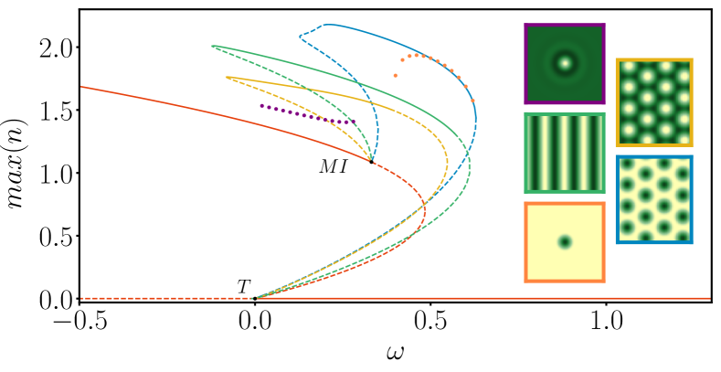
Figure 1: Bifurcation diagram of the homogeneous steady states $n^{*}$ (red lines) and stationary patterns of Eq. (1). The maximum value of the density $n(\vec{r})$ is plotted as a function of mortality $\omega$. Solid (dashed) lines indicate stable (unstable) solutions. The 2$d$ spatial distribution of each solution is shown in the corresponding inset: negative hexagons (yellow line), stripes (green line), and positive hexagons (blue line). Dots indicate the stable part of the branches of localized states: negative soliton (purple dots), and positive soliton (orange dots). Parameters: $a=1.39$, $b=1$, $\epsilon=1.15\times 10^{-2}$, $\alpha=-1.78$, $\delta=1.03\times 10^{-2}$, and $\beta=-1$.

Figure 2 shows the location of different bifurcation and stability domains in the two-parameter space ($\omega$,$a$), as identified from a linear stability analysis of the HSS against perturbations of the form $e^{\lambda t+i\vec{q}\cdot\vec{x}}$. It reveals that the unpopulated solution $n_{0}^{*}$ is unstable for $\omega<0$, leading to a homogeneous growth of the density until the solution $n_{+}^{*}$ is reached. This branch $n_{+}^{*}$ is stable against homogeneous perturbations $q=0$, where $q=\|\vec{q}\|$. However, for $\omega$ above a certain threshold $\omega_{c}$, it becomes unstable against modulations with a given critical wave number $q_{c}$, what is known as a modulation (or Turing) instability (MI). For values of $\omega>\omega_{c}$, the HSS $n_{+}^{*}$ remains unstable until the saddle node bifurcation (see Figs. 1 and 2). In the supercritical case, $a<0$, the homogeneous state becomes unstable at the MI and the region of instability persists until a second MI close to the transcritical bifurcation at $\omega=0$. The phase diagram in Fig. 2 reproduces all the qualitative features present in the ABD model (compare with Fig. S3 in Ref. Ruiz-Reynés et al. (2017)). Beyond the qualitative agreement, the shape and velocity of a front between the populated and unpopulated solutions, as well as the position in parameter space of the MI in the ABD model, can be quantitatively predicted by the reduced model if the full nonlocal term is kept, but this quantitative accuracy is partially lost when the expansion of the integral term is truncated linearly in $n_{t}$ and to fourth order in the gradients, which is the roughest approximation in our derivation.

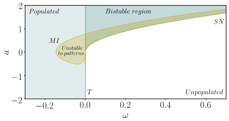
Figure 2: Phase diagram of the homogeneous steady states of Eq. (1). Blue line at $\omega=0$ signals the transcritical bifurcation of the zero solutions. For $a<0$, this bifurcation is supercritical and the populated solutions $n^{*}_{+}$ exist only for $\omega<0$. For $a>0$, the bifurcation is subcritical and the region of existence of $n^{*}_{+}$ extends to positive values of $\omega$ until the saddle-node bifurcation (SN) indicated by the green line. In the white region, the only possible solution is bare soil. In the light blue region, the only stable HSS is $n^{*}_{+}$, while in the dark blue region $n^{*}_{+}$ stably coexist with bare soil. The yellow line signals the modulation instability of $n^{*}_{+}$. In the yellow regions, $n^{*}_{+}$ is unstable to patterns. The region of existence of patterns extends beyond the yellow region. Parameters as in Fig. 1.

The nonlinear regimes of the dynamics can not be inferred just by the linear stability analysis. We use numerical continuation techniques to follow the stable and unstable parts of the branches of different patterns. Localized structures are obtained using numerical simulations, capturing only the stable part of the branch. Figure 1 shows the different patterns observed for different values of the growth rate $\omega$. Although the value of the parameters for which the different patterns appear does not precisely correspond with the ones in the ABD model Ruiz-Reynés et al. (2017), the type and sequence of patterns when the mortality is increased are the same, as expected from the general theory Gowda et al. (2014).

V EFFECTS OF CLONAL GROWTH

The term $\delta\norm*{\vec{\nabla}n_{t}}^{2}$, which originates from the distinctive mechanism of clonal growth, affects mainly the dynamics of fronts. This term contributes always to the velocity of a front in the direction from higher to lower densities. In the absence of the MI, using the perturbative method detailed in the Appendix, it is possible to calculate the contribution of this term to the velocity of a front between bare soil and the homogeneous populated state. The MI is not present when $\alpha=\beta=0$, which corresponds to the absence of long-range interactions, and the growth rate of perturbations with wave number $q$ goes as $-\epsilon q^{2}$, where the maximum growth rate corresponds to the homogeneous mode. In this case, as it can be seen in Fig. 3, the term with coefficient $\delta$ favors the expansion (i.e., increases the velocity) of the populated solution over the zero state, which we interpret as the result of the elongation of the rhizomes outward of the meadows. As a consequence, the position of the Maxwell point where the front has zero velocity moves to higher mortalities as compared to the same equation with $\delta=0$ Alvarez-Socorro et al. (2017), i.e. clonal-growth plants can colonize a new empty space under unfavorable conditions more efficiently than if the propagation is driven by seed dispersal (diffusion) only.

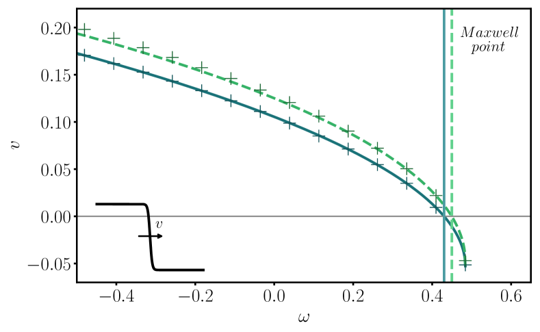
Figure 3: Velocity of a front between bare-soil and the homogeneous populated solution (in the absence of the MI) as a function of the mortality $\omega$. Crosses are the results of numerical simulations. The curve in blue (solid) corresponds to the analytical solution of Eq. (1) for $\alpha=\beta=\delta=0$ (see Appendix). The curve in green (dashed) is the velocity computed using the perturbative method detailed in the Appendix for $\alpha=\beta=0$ and to first order in $\delta$ for $\delta=1.03\times 10^{-2}$. Other parameters as in Fig. 1. The solid (dashed) vertical lines indicate the position of the Maxwell point for $\delta=0$ ($\delta=1.03\times 10^{-2}$).

Further increasing $\delta$ can have important effects on the dynamics of patterns. For instance, for large values of $\delta$ traveling patterns are observed as shown in Fig. 4. The figure shows a periodic pattern traveling to the right, whereas another solution (with shape related by the $x\rightarrow-x$ parity transformation) with velocity toward the left also exists. The velocity of the patterns grows, increasing $\delta$. Such parity-breaking bifurcation from steady to moving patterns is actually observed in the ABD model for low branching angles $\phi_{b}$. This is consistent with the relation between $\phi_{b}$ and $\delta$ derived in this work [Eq. (8)]. Thus, low branching angles, which are common for different species, can lead to bigger values of $\delta$, which can trigger this instability. The detailed analysis of the transition to moving patterns as well as other dynamical regimes of Eq. (1) will be studied elsewhere.

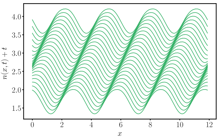
Figure 4: Space-time representation of a pattern of stripes traveling toward the right for $\omega=0$, $\alpha=-8$ and $\delta=15$. Other parameters as in Fig. 1. Densities at successive times are displaced vertically. For the same parameter values a parity-symmetric solution exists that travels toward the left.

VI CONCLUSIONS

Summarizing, we have proposed a simple model to describe the growth and dynamics of clonal-plant meadows. We have also derived the equation from a realistic model, providing analytical expressions for the effective parameters as a function of the biologically relevant parameters of the full model. The reduced model provides a qualitative description of clonal-growth plants, reproducing all the stationary spatial distributions and dynamical regimes. Moreover, beyond a qualitative description, accurate quantitative results can be obtained depending on the level of approximation of the non-local interacting terms. We expect this simple model, applicable to a wide variety of clonal plants, to allow deeper theoretical studies on the dynamics of clonal growth not tractable using a fully detailed model.

Appendix

In this Appendix we give details on the derivation of our simplified equation from the ABD model, and on the calculation of the velocity of a front using perturbative methods.

1 Derivation of the clonal-growth equation

We derive here our simplified equation for the spatial distribution of the density $n(\vec{r},t)$ of clonal-growth vegetation:

$$\partial_{t}n = -\omega n+an^{2}-bn^{3}+\epsilon\nabla^{2}n$$ (A1)

$$+ \alpha(\nabla^{2}n)n+\delta\norm*{\vec{\nabla}n}^{2}+\beta(\nabla^{4}n)n\ ,$$

starting from the more detailed and biologically motivated ABD model Ruiz-Reynés et al. (2017). This will allow us to give a one to one correspondence of the parameters in Eq. (A1) with biologically relevant parameters.

The ABD model, introduced in Ref. Ruiz-Reynés et al. (2017), describes the time evolution of the spatial and angular density of apices $n_{a}(\vec{r},\phi,t)$, where $\phi$ is the angle of the growth direction, and shoots $n_{s}(\vec{r},t)$, in a meadow,

$$\partial_{t}n_{a}(\vec{r},\phi,t) =-\omega_{d}[n_{t}]n_{a}(\vec{r},\phi,t)-\vec{v}(\phi)\cdot\vec{\nabla}n_{a}(\vec{r},\phi,t)$$

$$+ \frac{\omega_{b}}{2} \left(n_{a}(\vec{r},\phi+\phi_{b},t)+n_{a}(\vec{r},\phi-\phi_{b},t)\right),$$ (A2)

$$\partial_{t}n_{s}(\vec{r},t)= - \omega_{d}[n_{t}]n_{s}(\vec{r},t)+\frac{\nu}{\rho}\int_{0}^{2\pi}n_{a}(\vec{r},\phi,t)d\phi,$$ (A3)

where the growth-velocity vector is $\vec{v}=\nu(\cos\phi,\sin\phi)$ and $\vec{\nabla}=(\partial_{x},\partial_{y})$.

The death rate of the plant $\omega_{d}[n_{t}(\vec{r},t)]$ depends on the total density $n_{t}(\vec{r},t)=n_{s}(\vec{r},t)+N_{a}(\vec{r},t)$, where $N_{a}(\vec{r},t)=\int_{0}^{2\pi}n_{a}(\vec{r},\phi,t)d\phi$ is the total density of apices growing in all directions, as

$$\omega_{d}[n_{t}(\vec{r},t)]=\omega_{d0}+Bn^{2}_{t}+\iint\limits_{-\infty}^{+\infty}\mathcal{K}(\vec{r}-\vec{r}^{\prime})(1-e^{-a_{e}n_{t}(\vec{r}^{\prime})})d\vec{r}^{\prime},$$ (A4)

where the kernel $\mathcal{K}$ is the difference of two normalized Gaussians $\mathcal{G}$ of different strengths $\kappa$ and $\mu$, and widths $\sigma_{\kappa}$ and $\sigma_{\mu}$:

$$\mathcal{K}(\vec{r})=\kappa\mathcal{G}(\sigma_{\kappa},\vec{r})-\mu\mathcal{G}(\sigma_{\mu},\vec{r})\ .$$ (A5)

We first obtain a relationship for the steady homogeneous solutions, $n_{s}(\vec{r},t)=n_{s}^{*}$ and $n_{a}(\vec{r},\phi,t)=n_{a}^{*}$, from which $N_{a}^{*}=2\pi n_{a}^{*}$. From Eq. (1), we obtain that $(-\omega_{d}[n_{t}]+\omega_{b})n_{a}^{*}=0$, which, for a populated solution, implies equality between branching and death rates, $\omega_{b}=\omega_{d}[n_{t}]$. Using this into the steady state of Eq. (A3), we get $(\nu/\rho)N_{a}^{*}-w_{b}n_{s}^{*}=0$, or $n_{s}^{*}=(\nu/\rho\omega_{b})N_{a}^{*}$. Inserting in $n_{t}^{*}=n_{s}^{*}+N_{a}^{*}$, we find the following relationship between the total-apex density and the total plant density:

$$N^{*}_{a}=\frac{\rho\omega_{b}}{\nu+\rho\omega_{b}}n_{t}^{*}\equiv\eta n_{t}^{*}.$$ (A6)

To eliminate the angular dependence in Eqs. (1) and (A3), and find a single equation for the total density, we first write the density of apices as a Fourier series in the angle $\phi\in[0,2\pi]$:

$$n_{a}(\vec{r},\phi,t)=\frac{a_{0}(\vec{r},t)}{2}$$

$$+\sum_{m=1}^{\infty}\left(a_{m}(\vec{r},t)\cos(m\phi)+b_{m}(\vec{r},t)\sin(m\phi)\right).\$$ (A7)

Note that $\pi a_{0}(\vec{r},t)=N_{a}(\vec{r},t)$. Using Eqs. (1) and (A7), we find the evolution equations for all the amplitudes $a_{m}$, $b_{m}$. This gives an infinite hierarchy of coupled equations such that modes $m$ are coupled to modes $m+1$. From numerical simulations and the linear stability analysis one can check, however, that modes with $m>1$ are not contributing substantially to the dynamics. Therefore these terms can be neglected. As a second approximation we assume that the relation in Eq. (A6), obtained for the populated HSS, is also valid for all $\vec{r}$ and $t$ in any heterogeneous spatial distribution. We have checked the accuracy of this approximation using numerical simulation. The maximum error in a stationary pattern is less than $10\%$ of the total density of apices.

With these approximations Eqs. (1) and (A3) can be simplified to three equations (for $n_{t}$, $a_{1}$, and $b_{1}$). Defining $\vec{a}\equiv(a_{1},b_{1})$, $A=\norm*{\vec{a}}$ and $\theta=\arctan(b_{1}/a_{1})$, they can be written as

$$\partial_{t}n_{t} =(\omega_{b}-\omega_{d}[n_{t}])n_{t}-\frac{\nu\pi}{\eta}\nabla\cdot\vec{a}$$ (A8)

$$\partial_{t}A =(\omega_{b}\cos\phi_{b}-\omega_{d}[n_{t}])A-\frac{\nu\eta}{2\pi}\norm*{\vec{\nabla}n_{t}}\cos(\theta-\gamma)$$ (A9)

$$\partial_{t}\theta =\frac{\nu\eta}{2\pi}\frac{\norm*{\vec{\nabla}n_{t}}}{A}\sin(\theta-\gamma)\ ,$$ (A10)

where $\gamma(\vec{r},t)=\arctan(\partial_{y}n_{t}/\partial_{x}n_{t})$ is the angle that the gradient of the total density forms with the $x$ axis. From Eq. (A10), the evolution of the system will drive the angle $\theta$ to the stable fixed point $\theta=\gamma+\pi$. This means that, in the long run, the density gradient and the vector $\vec{a}$ have opposite directions: $\vec{a}=-C\vec{\nabla}n_{t}$, or $A=C\norm*{\vec{\nabla}n_{t}}$, with $C$ a positive constant. Introducing this result in the Fourier series given by Eq. (A7) truncated at $m=1$, the density of apices takes the following form:

$$n_{a}(\vec{r},\phi,t)=\frac{N_{a}(\vec{r},t)}{2\pi}+C\norm*{\vec{\nabla}n_{t}(\vec{r},t)}\cos(\phi-\gamma(\vec{r},t)-\pi)\ .$$ (A11)

In regions where the total density is homogeneous, $\vec{\nabla}n_{t}$ is zero and the densities of apices growing in all directions are equal and proportional to the total density of apices $N_{a}$. On the other hand, in regions where $\vec{\nabla}n_{t}\neq 0$, there is an angular modulation of the density. For example, considering a circular patch, those apices growing outward (normal to the vegetation border) are denser while those growing inward are depleted, as can be seen in Fig. 5 from numerical simulations. The same effect can be observed for different spatial distributions as shown in Ref. Ruiz-Reynés et al. (2019). The value of $C$ is related to the amplitude of the modulation at the borders of the patch, and in general it will be a complicated function of $n_{t}$ and its derivatives. Considering only the leading terms of a power expansion of $C(n_{t},\vec{\nabla}n_{t},...)$ we take:

$$\vec{a}=\frac{\eta}{\pi}\vec{a}^{\prime}=-\frac{\eta}{\pi}(c_{0}+c_{1}n_{t})\vec{\nabla}n_{t}\ ,$$ (A12)

where $c_{0}$ and $c_{1}$ are constants to be determined. Introducing Eq. (A12) in Eq. (A8), one obtains a closed equation for the total density $n_{t}$:

$$\partial_{t}n_{t}=(\omega_{b}-\omega_{d}[n_{t}])n_{t}+\nu(c_{0}\nabla^{2}n_{t}+c_{1}\norm*{\vec{\nabla}n_{t}}^{2}+c_{1}n_{t}\nabla^{2}n_{t})\ .$$ (A13)

This equation is used in the main text, together with an expansion of the integral in $\omega_{d}[n_{t}]$ and identifying $n$ with the total plant density $n_{t}$, to establish the simplified model Eq. (A1).

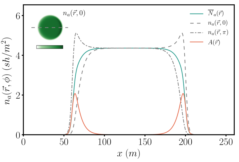
Figure 5: Densities (in shoots per square meter, sh/m²) of apices of a circular domain invading the unpopulated solution for the ABD model with parameters appropriate for the seagrass Posidonia oceanica but without nonlocal interactions Ruiz-Reynés et al. (2017): $\omega_{b}=0.06$ year^-1, $\omega_{d0}=0.038$ year^-1 , $\nu=6.11$ cm/year, $\rho=2.87$ cm, $\phi_{b}=45^{\circ}$, $b=1.25$ cm⁴year^-1, $\kappa=0.048$ year^-1, $\sigma_{\kappa}=0$ cm, $a=27.38$ cm², $\sigma_{\mu}=0$cm, $\mu=\omega_{d0}$. The inset in green represents the density of apices growing to the right ($\phi=0$), and the dashed line indicates the cut shown in the main plot. The blue line represents the mean angular density of apices ($\bar{N}_{a}=N_{a}/2\pi$). The dashed (dot-dashed) line shows the density of apices growing to the right (left). The red line shows the amplitude $A$ of the first mode ($m=1$) in Eq. (A7).

Parameters $c_{0}$ and $c_{1}$ have not been determined so far. It is possible to determine their value close to the Maxwell point where a front between the populated HSS and bare soil is at rest. Assuming such a stationary front and introducing Eq. (A12) in Eq. (A9), recalling that $\theta=\gamma+\pi$, one obtains the following expression:

$$\bigg{\{}(\omega_{b}\cos\phi_{b}-\omega_{d}[n_{t}])(c_{0}+c_{1}n_{t})+\frac{\nu}{2}\bigg{\}}\frac{\eta}{\pi}\norm*{\vec{\nabla}n_{t}}=0.$$ (A14)

A priori the front profile is not known, however, we know it connects with the populated solution on one side and with the unpopulated solution on the other, so we can write $n_{t}=n^{*}_{t}+\varepsilon e^{\lambda x}$, where $n_{t}^{*}$ is zero for the unpopulated solution at one side and takes the value of the stationary homogeneous density $n_{t,M}^{*}$ for the populated solution at the Maxwell point ($\omega_{d0}=\omega_{d0,M}$) at the other. Here $\lambda$ is the spatial eigenvalue of each solution. Introducing these expressions in Eq. (A14), at the lowest order in $\varepsilon$ we obtain

$$c_{0} =\frac{\nu}{2(\omega_{d0,m}-\omega_{b}\cos\phi_{b})},$$ (A15)

$$c_{1} =\frac{\nu}{2n_{t}^{*}}\left(\frac{1}{\omega_{b}\cos\phi_{b}-\omega_{d0,M}}-\frac{1}{\omega_{b}\cos\phi_{b}-\omega_{b}}\right).$$ (A16)

For the unpopulated solution $n_{t}^{*}=0$ and the populated one $n_{t}^{*}=n_{t,M}^{*}$.

The last approximation on the derivation consists of taking the moment expansion of the integral term in Eq. (A4). We can approximate the exponential term at first order and use the convolution theorem to write:

$$\iint\limits_{-\infty}^{+\infty}\mathcal{K}(\vec{r}-\vec{r}^{\prime})(1-e^{-a_{e}n_{t}(\vec{r}^{\prime},t)})d\vec{r}^{\prime}$$

$$\simeq a_{e}\iint\limits_{-\infty}^{+\infty}\mathcal{K}(\vec{r}-\vec{r}^{\prime})n_{t}(\vec{r}^{\prime},t)d\vec{r}^{\prime}$$

$$=\frac{a_{e}}{(2\pi)^{2}}\iint\limits_{-\infty}^{+\infty}e^{i\vec{q}\cdot\vec{r}}\tilde{\mathcal{K}}(\vec{q})\tilde{n}_{t}(\vec{q},t)d\vec{q},$$ (A17)

where $\tilde{\mathcal{K}}(\vec{q})$ and $\tilde{n}_{t}(\vec{q})$ are the Fourier transforms of the kernel and the total density. Due to the symmetry of the kernel, $\tilde{\mathcal{K}}(\vec{q})=\tilde{\mathcal{K}}(q)$, where $q=\|\vec{q}\|$. We use a Taylor expansion to write the kernel in terms of its derivatives evaluated at the origin. Only even derivatives are non-zero:

$$\frac{a_{e}}{(2\pi)^{2}}\iint\limits_{-\infty}^{+\infty}e^{i\vec{q}\cdot\vec{r}}\sum_{j=0}^{\infty}\frac{1}{j!}\frac{d^{j}\tilde{\mathcal{K}}(q)}{dq^{j}}\bigg{|}_{q=0}q^{j}\tilde{n}_{t}(\vec{q},t)d\vec{q}$$

$$=\frac{a_{e}}{(2\pi)^{2}}\sum_{j=0}^{\infty}\frac{1}{(2j)!}\frac{d^{2j}\tilde{\mathcal{K}}(q)}{dq^{2j}}\bigg{|}_{q=0}\iint\limits_{-\infty}^{+\infty}e^{i\vec{q}\cdot\vec{r}}q^{2j}\tilde{n}_{t}(\vec{q},t)d\vec{q}$$

$$=a_{e}\sum_{j=0}^{\infty}d_{j}\nabla^{2j}n_{t}(\vec{r},t),$$ (A18)

where

$$d_{j}=\frac{(-1)^{j}}{(2j)!}\frac{d^{2j}\tilde{\mathcal{K}}(q)}{dq^{2j}}\bigg{|}_{q=0}.$$ (A19)

The coefficients $d_{j}$ can be computed from Eq. (A19) or in terms of the moments of the kernel in radial coordinates:

$$d_{j} = \frac{(-1)^{j}}{(2j)!}\frac{d^{2j}\tilde{\mathcal{K}}(q)}{dq^{2j}}\bigg{|}_{q=0}=\frac{(-1)^{j}}{(2j)!}\frac{d^{2j}}{dq^{2j}}\iint\limits_{-\infty}^{+\infty}e^{-i\vec{q}\cdot\vec{r}}\mathcal{K}(\vec{r})d\vec{r}\bigg{|}_{q=0}$$ (A20)

$$= \frac{(-1)^{j}}{(2j)!}\frac{d^{2j}}{dq^{2j}}\int\limits_{0}^{\infty}\mathcal{K}(r)\int\limits_{0}^{2\pi}e^{-iqr\cos(\theta-\phi)}d\theta rdr\bigg{|}_{q=0}$$

$$= \frac{(-1)^{j}}{(2j)!}\frac{d^{2j}}{dq^{2j}}\int\limits_{0}^{\infty}\mathcal{K}(r)2\pi J_{0}(qr)rdr\bigg{|}_{q=0}$$

$$= \frac{(-1)^{j}}{(2j)!}2\pi J_{0}^{(2j)}(0)\int\limits^{\infty}_{0}r^{2j+1}\mathcal{K}(r)dr,$$

where $J_{0}^{(2j)}(0)$ is the $2j$th derivative of the Bessel function $J_{0}$ of the first kind evaluated at the origin.

2 Calculation of the velocity of a front using a perturbative method

We consider Eq. (1) in the case of $\alpha=\beta=0$. Thus, the dispersion relation changes with the wave number $q$ as $-\epsilon q^{2}$, the maximum growth rate corresponds to $q=0$ and the modulational instability is absent. In this case, solutions consisting of an unpopulated and a populated homogeneous solutions separated by a front that moves at constant velocity $v$ exist, so that one can rewrite the equation in one dimension as a time-independent one in the comoving reference frame $x\rightarrow x-vt$. Positive velocity indicates motion toward larger $x$ values. We want to analyze perturbatively the effect of the presence of a small parameter $\delta$ on the motion of the front, similarly to the approach in Ref. Löber et al. (2012). To this end we write $\delta\rightarrow\xi\delta$, with $\xi$ small, to emphasize that $\delta$ is small. At the end of the calculation we can set back $\xi=1$. The steady equation in the comoving frame reads:

$$0=-\omega n+an^{2}-bn^{3}+\epsilon\partial_{x}^{2}n+v\partial_{x}n+\xi\delta(\partial_{x}n)^{2}\ .$$ (A21)

For $\xi=0$, the analytical solution $n_{0}(x)$ that connects the populated $n_{+}^{*}$ state for $x\rightarrow-\infty$ ($n_{0}(x\rightarrow-\infty)=n_{+}^{*}$) with the bare-soil solution when $x\rightarrow\infty$ ($n_{0}(x\rightarrow\infty)=0$) is

$$n_{0}(x)=\frac{n^{*}_{+}}{2}\left(1-\tanh(\frac{n^{*}_{+}}{2}\sqrt{\frac{b}{2\epsilon}}x)\right),\$$ (A22)

with velocity $v_{0}=\sqrt{\frac{\epsilon b}{2}}(n^{*}_{+}-2n^{*}_{-})$, where $n^{*}_{\pm}=(a\pm\sqrt{a^{2}-4\omega})/(2b)$. Thus, writing $n=n_{0}+\xi n_{1}+\mathcal{O}(\xi^{2})$ and $v=v_{0}+\xi v_{1}+\mathcal{O}(\xi^{2})$ and substituting in Eq. (A21), we obtain to first order in $\xi$:

$$0 =(-\omega+2an_{0}-3bn_{0}^{2})n_{1}$$

$$+\epsilon\partial_{x}^{2}n_{1}+v_{0}\partial_{x}n_{1}+\delta(\partial_{x}n_{0})^{2}+v_{1}\partial_{x}n_{0}.$$ (A23)

Defining the operator $\hat{\mathcal{L}}=(-\omega+2an_{0}-3bn_{0}^{2})+\epsilon\partial_{x}^{2}+v_{0}\partial_{x}$ one can write

$$\hat{\mathcal{L}}n_{1}=-\delta(\partial_{x}n_{0})^{2}-v_{1}\partial_{x}n_{0}.$$ (A24)

Let $\langle f\big{|}g\rangle=\int_{-\infty}^{\infty}f(x)g(x)dx$ be the inner product, $\hat{\mathcal{L}}^{\dagger}$ the adjoint of $\hat{\mathcal{L}}$, and $w(x)=\exp(\frac{v_{0}}{\epsilon}x)\partial_{x}n_{0}$ the neutral mode of $\hat{\mathcal{L}}^{\dagger}$ ($\hat{\mathcal{L}}^{\dagger}w=0$). We can apply the solvability condition $\langle w\big{|}\hat{\mathcal{L}}n_{1}\rangle=\langle w\big{|}f(x)\rangle$, so that $\langle\hat{\mathcal{L}}^{\dagger}w\big{|}n_{1}\rangle=\langle w\big{|}f(x)\rangle$ and $0=\langle w\big{|}f(x)\rangle$, to write

$$\langle w\big{|}-\delta(\partial_{x}n_{0})^{2}-v_{1}\partial_{x}n_{0}\rangle=0.$$ (A25)

Thus, we can determine the contribution to the velocity due to the effect of $\delta$:

$$v_{1}=\frac{\langle w\big{|}-\delta(\partial_{x}n_{0})^{2}\rangle}{\langle w\big{|}\partial_{x}n_{0}\rangle}.$$ (A26)

Solving the integrals in Eq. (A26), we obtain

$$v_{1}=\frac{\delta\left(\frac{v_{0}^{4}}{\epsilon^{2}}-\frac{5v_{0}^{2}bn_{+}^{*2}}{2\epsilon}+b^{2}n_{+}^{*4}\right)}{10\sqrt{2b\epsilon}\left(\frac{bn_{+}^{*2}}{2}-\frac{v_{0}^{2}}{\epsilon}\right)}.$$ (A27)

The unperturbed velocity $v_{0}$ and the one with the first order correction in $\delta$ ($v=v_{0}+v_{1}$, since $\xi=1$) are plotted in Fig. (3). The effect of $\delta$ is to increase $v$ in the positive direction, i.e. to speed up the advance of the populated state onto the unpopulated one.

References

- Meron (2015) E. Meron, Nonlinear Physics of Ecosystems (CRC Press, Boca Raton, 2015).
- Gowda et al. (2014) K. Gowda, H. Riecke, and M. Silber, Physical Review E 89, 022701 (2014).
- Rietkerk and van de Koppel (2008) M. Rietkerk and J. van de Koppel, Trends in Ecology & Evolution 23, 169 (2008).
- Getzin et al. (2016) S. Getzin, H. Yizhad, B. Bell, T. E. Erickson, A. C. Postle, I. Katra, O. Tzuk, Y. R. Zelnik, K. Wiegand, T. Wiegand, and E. Meron, Proceedings of the National Academy of Sciences 113, 3551 (2016).
- Ruiz-Reynés et al. (2017) D. Ruiz-Reynés, D. Gomila, T. Sintes, E. Hernández-García, N. Marbà, and C. M. Duarte, Science Advances 3, e1603262 (2017).
- Cross and Hohenberg (1993) M. C. Cross and P. C. Hohenberg, Rev. Mod. Phys. 65, 851 (1993).
- Lefever and Lejeune (1997) R. Lefever and O. Lejeune, Bulletin of Mathematical Biology 59, 263 (1997).
- Lejeune and Tlidi (1999) O. Lejeune and M. Tlidi, Journal of Vegetation Science 10, 201 (1999).
- Lejeune et al. (2002) O. Lejeune, M. Tlidi, and P. Couteron, Phys. Rev. E 66, 010901(R) (2002).
- Fernandez-Oto et al. (2019) C. Fernandez-Oto, O. Tzuk, and E. Meron, Phys. Rev. Lett. 122, 048101 (2019).
- Paulau et al. (2014) P. V. Paulau, D. Gomila, C. López, and E. Hernández-García, Phys. Rev. E 89, 032724 (2014).
- Routledge (1990) R. D. Routledge, Journal of Applied Probability 27, 1 (1990).
- Sintes et al. (2005) T. Sintes, N. Marbà, C. M. Duarte, and G. A. Kendrick, Oikos 108, 165 (2005).
- Murray (2002) J. D. Murray, Mathematical Biology I: An Introduction, Vol. 17 of Interdisciplinary Applied Mathematics (Springer, New York, 2002).
- Alvarez-Socorro et al. (2017) A. J. Alvarez-Socorro, M. G. Clerc, G. González-Cortés, and M. Wilson, Phys. Rev. E 95, 010202(R) (2017).
- Löber et al. (2012) J. Löber, M. Bär, and H. Engel, Phys. Rev. E 86, 066210 (2012).
- Ruiz-Reynés et al. (2019) D. Ruiz-Reynés, and D. Gomila, Phys. Rev. E 100, 052208 (2019).