Computation of conformal invariants

^aDepartment of Mathematics, Statistics and Physics, Qatar University, Doha, Qatar.

mms.nasser@qu.edu.qa

^bDepartment of Mathematics and Statistics, University of Turku, Turku, Finland.

vuorinen@utu.fi

Keywords.  Conformal capacity; hyperbolic capacity; elliptic capacity; boundary integral equations; numerical conformal mapping

MSC.   65E05; 30C85; 31A15

1 Introduction

During the past fifty years conformal invariants have become crucial tools for complex analysis. Most important of these invariants are the conformal capacity, the harmonic measure, the extremal length, and the hyperbolic distance [1, 15, 21, 39]. But this is not all: the generalized capacity, the transfinite diameter, the reduced extremal length, the hyperbolic area, and the modulus metric [12, 22, 42, 43, 44] are some additional examples, see [20, Ch 10]. Some of the many applications of these tools are discussed in the articles of the handbook [25]. In view of the plenitude of these applications, it is surprising that these invariants can be expressed explicitly only in very few special cases. Sometimes rudimentary upper or lower bounds for conformal invariants in terms of less involved comparison functions can provide important steps in proofs.

At the same time it seems that the full power of conformal invariance remains unused. One reason for this is that the analytic expressions for conformal invariants are usually too complicated for pen and paper calculations and the existing computational methods are scattered throughout the mathematical literature: the way from theory to practical experimentation is too long. On the other hand, the creators of the existing computational methods may not be aware of the scope of applicability of their methods in theoretical studies: the way from experiments to theory is also long. If the distance from theory to experiments could be made shorter, a theoretical researcher could easily experiment with the dependence of a problem under perturbation of geometry and vice versa a computational scientist would find new types of benchmark problems and areas of application.

With the above ideas as our guiding principles, we have written a series of papers of which the present one is devoted to doubly connected domains [36, 35]. As far as we know, our work is the first attempt to provide computational tools for a wide class of conformal invariants with the feature that modification of geometry is simple. The method we use was developed and implemented by the first author [30] and we apply it to study several computational problems never studied before and we also compare its performance to several results in the literature. As test problems we use the computation of condenser capacity, a topic studied by the second author in several papers [17, 18, 19].

A condenser is a pair $(D,C)$ where $D$ is an open set in $\mathbb{R}^{2}$ and $C\subset D$ is compact. In our study we assume that the topology is simple but still general enough for most applications: the sets $\partial D$ and $\partial C$ are connected sets, each set is a piecewise smooth Jordan curve. The cases for which the sets $\partial D$ and $\partial C$ are slits will be also considered.

The conformal capacity, or capacity for short, is defined by [12]

$${\rm{cap}}(D,C)=\int_{D}|\nabla u|^{2}\,dm$$ (1)

where $u:D\to\mathbb{R}$ is a harmonic function with $u(x)\geq 1\,$ for all $x\in C\,$ and $u(x)\to 0\,$ for $x\to\partial D\,.$ The domain $G=D\setminus C$ is called the field of the condenser and the closed sets $C$ and $D^{c}$ are called the plates of the condenser. Then, the capacity ${\rm{cap}}(D,C)$ may alternatively be written as ${\rm{cap}}(G)$.

In literature, only very few formulas are given for the capacities of concrete condensers. Numerical methods are therefore needed to compute the value of (1). Our problem is reduced to the classical problem of solving numerically the Dirichlet boundary value problem for the Laplace equation. Moreover, by the Dirichlet principle [15, pp. 447-456], the extremal function $u_{0}$ is harmonic and minimizes the integral [1], [15, pp.441-456]:

$$\int_{D}|\nabla u_{0}|^{2}\,dm=\inf\{\int_{D}|\nabla u|^{2}\,dm\}$$ (2)

where the infimum is taken over all $C_{o}(D)$ functions with the indicated Dirichlet boundary values. The capacity of condensers is invariant under conformal mappings, and hence domains with difficult geometry can be treated using conformal mappings [2, 11, 12, 26, 38, 40, 42, 44]. See also [6, 10, 14].

Before proceeding to the contents of our work a few general remarks about the literature we know about may be in order. Because of the wide scope of conformal invariants, relatively few cases exist where “the right answer” is known. In cases for which the analytic formulas are unknown, the computational performance may be analysed by observing convergence features of the results under successive refinements of the numerical model, and error estimates maybe based on general theory. In those relatively few cases we have found in the literature where the analytic formula is known, the true error estimate may be given. Sometimes a high accuracy can be achieved, say 12 decimal places, but the dilemma is that if the geometry of the problem is smoothly changed a bit, the method might not be applicable at all.

Section 2 summarizes our computational workhorse, the boundary integral method geared for the capacity computation of ring domains, which will be applied in several later sections, sometimes together with auxiliary procedures. In Section 3 we consider ring domains for which the exact value of capacity is known and investigate the performance of our method. Sections 4, 5, and 6 deal with condensers whose one or two complementary components are slits—these are well-known examples of computationally challenging problems and we use here auxiliary conformal mapping to overcome computational difficulties. Section 7 deals with the case when both complementary components of a ring domain are thin rectangles. In Section 8, we consider the numerical computation of the hyperbolic capacity and the elliptic capacity of compact and closed sets. The final Section 9 gives some concluding remarks and information about the access to our MATLAB software.

2 Conformal mapping onto annulus

2.1 Ring domains.

A domain $G$ in the extended complex plane $\overline{\mathbb{C}}=\mathbb{C}\cup\{\infty\}\,,$ whose complement $\overline{\mathbb{C}}\setminus G$ has two components, is called a ring domain or, briefly, a ring. It is a classical fact that a ring can be mapped by a conformal map onto an annulus $\{z:q<|z|<1\}\,,q\in(0,1)\,.$ A ring $R$ is the simplest example of a condenser and its capacity is given by [12], [15, p. 132-133]

$${\rm cap}(R)=\frac{2\pi}{\log(1/q)}\,.$$

The number $\log(1/q)$ is called the modulus of the ring, i.e.,

$$M(R)=\log(1/q)=\frac{2\pi}{\mathrm{cap}(R)}\,.$$ (3)

Because of the conformal invariance of the capacity, this definition is independent of the conformal map. For the computation of the capacity we will often use an auxiliary conformal mapping to avoid computational singularities.

In this section we describe the method of our numerical work, based on the solution of the boundary integral equation with the generalized Neumann kernel [30, 45]. The integral equation has been applied to calculate conformal mappings onto several canonical domains [28, 31, 32]. We review the application of the integral equation to compute the conformal mapping from doubly connected domains onto an annulus $\{z:q<|z|<1\},q\in(0,1)$, and present the MATLAB implementation of the method. In later sections we will apply this method for capacity computation of several condensers, in particular, we will consider several types of rings with a simple geometric structure.

2.2 The generalized Neumann kernel.

Let $G$ be a bounded or an unbounded doubly connected domain bordered by

$$\Gamma=\partial G=\Gamma_{1}\cup\Gamma_{2}$$

where each of the boundary components $\Gamma_{1}$ and $\Gamma_{2}$ is a closed smooth Jordan curve. We choose the orientation of boundary $\Gamma$ such that when we proceed along $\Gamma\,,$ the domain $G$ is always on the left side. If $G$ is bounded, then $\Gamma_{1}$ is the external boundary and $\Gamma_{2}$ is contained in the bounded domain whose boundary is $\Gamma_{1}$. The complement $\overline{\mathbb{C}}\backslash\overline{G}$ of the domain $G$ with respect to the extended complex plane $\overline{\mathbb{C}}$ consists of two simply connected domains $G_{1}$ on the right of $\Gamma_{1}$ and $G_{2}$ on the right of $\Gamma_{2}$. The domain $G_{2}$ is bounded and the domain $G_{1}$ is unbounded with $\infty\in G_{1}$. Further, we assume that $\alpha$ is an auxiliary given point in the domain $G$ and $z_{2}$ is an auxiliary given point in the simply connected domain $G_{2}$. When $G$ is unbounded, then $\infty\in G$ and the two domains $G_{1}$ and $G_{2}$ are bounded. We assume that $z_{1}$ and $z_{2}$ are auxiliary given points in the simply connected domains $G_{1}$ and $G_{2}$, respectively. See Figure 1.

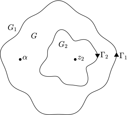
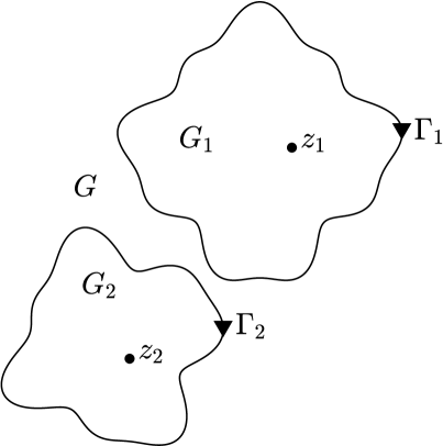
Figure 1: An example of a bounded doubly connected domain (left) and an unbounded doubly connected domain (right).

We parametrize each boundary component $\Gamma_{j}$ by a $2\pi$-periodic complex function $\eta_{j}(t)$, $t\in J_{j}:=[0,2\pi]$, $j=1,2$. We assume that each of these functions $\eta_{j}(t)$ is twice continuously differentiable with $\eta^{\prime}(t)\neq 0$ (the presented method can be applied also if the curve $\Gamma_{j}$ has a finite number of corner points but no cusps [34]). Then we define the total parameter domain $J$ as the disjoint union of the two intervals $J_{1}=[0,2\pi]$ and $J_{2}=[0,2\pi]$, i.e., $J=J_{1}\sqcup J_{2}=\cup_{j=1}^{2}\{(t,j)\;:\;t\in J_{j}\}$. The elements of the total parameter domain $J$ are ordered pairs $(t,j)$ where $t$ is a real number in $[0,2\pi]$ and the index $j$ is an integer indicating the interval $J_{j}$ containing $t$ [30]. Hence, the boundary $\Gamma$ can be parametrized by

$$\eta(t,j)=\eta_{j}(t),\quad t\in J_{j},\quad j=1,2.$$ (4)

For a given $t$, the index $k$ for which the interval $J_{k}$ contains $t$ will be always clear from the context, see e.g., [28, 30, 32, 33, 45]. So the pair $(t,k)$ in the left-hand side of (4) will be replaced by $t$ and a parametrization of the whole boundary $\Gamma$ can be defined on $J$ by

$$\eta(t)=\left\{\begin{array}[]{l@{\hspace{0.5cm}}l}\eta_{1}(t),\hfil\hskip 14.22636pt&t\in J_{1},\\ \eta_{2}(t),\hfil\hskip 14.22636pt&t\in J_{2}.\\ \end{array}\right.$$ (5)

We denote by $H$ the space of all functions of the form

$$\rho(t)=\left\{\begin{array}[]{l@{\hspace{0.5cm}}l}\rho_{1}(t),\hfil\hskip 14.22636pt&t\in J_{1},\\ \rho_{2}(t),\hfil\hskip 14.22636pt&t\in J_{2},\\ \end{array}\right.$$

where $\rho_{1}(t)$ and $\rho_{2}(t)$ are $2\pi$-periodic Hölder continuous real functions on $J_{1}$ and $J_{2}$, respectively.

Let $A$ be the complex function [30]

$$A(t)=\left\{\begin{array}[]{l@{\hspace{0.5cm}}l}e^{\mathrm{i}(\frac{\pi}{2}-\theta(t))}(\eta(t)-\alpha),\hfil\hskip 14.22636pt&{\rm if\;}G{\rm\;is\;bounded},\\ e^{\mathrm{i}(\frac{\pi}{2}-\theta(t))},\hfil\hskip 14.22636pt&{\rm if\;}G{\rm\;is\;unbounded},\\ \end{array}\right.$$ (6)

where $\theta$ is a real function with constant value on each interval $J_{j}$, i.e.,

$$\theta(t)=\theta_{j}\qquad{\rm for}\quad t\in J_{j}$$

and $\theta_{j}$ is a real constant, $j=1,2$. The generalized Neumann kernel $N(s,t)$ is defined for $(s,t)\in J\times J$ by

$$N(s,t):=\frac{1}{\pi}{\rm Im}\,\left(\frac{A(s)}{A(t)}\frac{\dot{\eta}(t)}{\eta(t)-\eta(s)}\right).$$ (7)

The kernel $N(s,t)$ is continuous [45]. Hence, the integral operator ${\bf N}$ defined by

$${\bf N}\rho(s):=\int_{J}N(s,t)\rho(t)dt,\quad s\in J,$$

is compact. The integral equation with the generalized Neumann kernel involves also the following kernel

$$M(s,t):=\frac{1}{\pi}{\rm Re}\,\left(\frac{A(s)}{A(t)}\frac{\dot{\eta}(t)}{\eta(t)-\eta(s)}\right),\quad(s,t)\in J\times J,$$ (8)

which has a singularity of cotangent type [45]. The integral operator ${\bf M}$ defined on $H$ by

$${\bf M}\rho(s):=\int_{J}M(s,t)\rho(t)dt,\quad s\in J,$$

is singular, but is bounded on $H$ [45]. For more details, see [45].

For the above function $A$ defined by (6), the following integral equation

$$({\bf I}-{\bf N})\rho=-{\bf M}\gamma$$ (9)

is uniquely solvable for any real function $\gamma$ in $H$ [29]. Furthermore, if $\rho$ is the unique solution of the boundary integral equation (9), then the real function $h$ defined by

$$h=[{\bf M}\rho-({\bf I}-{\bf N})\gamma]/2$$ (10)

is a piecewise constant function on the boundary $\Gamma$, i.e.,

$$h(t)=h_{j}\qquad{\rm for}\quad\eta(t)\in\Gamma_{j}$$

where $h_{j}$ is a real constant, $j=1,2$ [29]. Moreover,

$$f(\eta(t))=\frac{\gamma(t)+h(t)+\mathrm{i}\rho(t)}{A(t)},\quad\eta(t)\in\Gamma,$$ (11)

are boundary values of an analytic function $f$ in the doubly connected domain $G$ such that $f(\infty)=0$ when $G$ is unbounded. For more details, see [29, 30] and the references cited therein.

2.3 Numerical solution of the integral equation

The MATLAB function fbie in [30] provides us with an efficient and fast method for solving the boundary integral equation (9). The function fbie is based on discretizing the boundary integral equation (9) using the Nyström method with the trapezoidal rule [4, 3, 41]. This discretization leads to a non-symmetric linear system. Then, the MATLAB function $\mathtt{gmres}$ is used to solve the linear system. The matrix-vector multiplication in the GMRES method is computed using the MATLAB function $\mathtt{zfmm2dpart}$ in the toolbox $\mathtt{FMMLIB2D}$ [16]. The function fbie provides us also with approximations to the piecewise constant function $h$ in (10). The computational cost for the overall method is $O(n\log n)$ operations where $n$ (an even positive integer) is the number of nodes in each of the intervals $J_{1}$ and $J_{2}$.

For the accuracy of the obtained numerical results, it is known that the order of the convergence of the Nyström method depends on the order of convergence of the used quadratic method [3]. The quadratic method used in the function fbie is the trapezoidal rule which gives surprisingly accurate numerical results for periodic functions [3, 41]. In view of of (7) and (8), the smoothness of the two kernels $N(s,t)$ and $M(s,t)$ depends on the smoothness of the parametrization function $\eta(t)$. Similarly, in this paper, the function $\gamma$ on the right-hand side of the integral equation (9) will be defined in terms of $\eta(t)$. Hence, the smoothness of the function $\gamma$ will depend also on the smoothness of the boundary $\Gamma$. Thus, the order of convergence of the trapezoidal rule depends on the smoothness of the boundary $\Gamma$ of the domain $G$. For domain with smooth boundaries, we use the trapezoidal rule with equidistant nodes. The integrand in the integral equation (9) will be $C^{\infty}$ smooth if the boundaries of the domains are $C^{\infty}$ smooth. Hence the rate of convergence of the numerical method is $O(e^{-cn})$ with a positive constant $c$ (see [24, p. 223]). If the boundary is $C^{q+2}$ smooth $(q\geq 0)$, then the rate of convergence of the numerical method is $O(1/n^{q})$ [23]. For domains with corners (excluding cusps), the derivatives of the solution $\rho(t)$ of the boundary integral equation (9) have a discontinuity at the corner points. Thus, only poor convergence can be achieved if the trapezoidal rule with equidistant nodes is used. For such domains, accurate results can be obtained if we use the trapezoidal rule with a graded mesh [23]. Such a graded mesh can be obtained by substituting a suitable new variable in the integral equation such that the discontinuity in the derivatives of $\rho(t)$ is removed [23, 27].

To use the MATLAB function fbie, the vectors et, etp, A, and gam that contain the discretizations of the functions $\eta(t)$, $\eta^{\prime}(t)$, $A(t)$, and $\gamma(t)$, respectively, will be stored in MATLAB. Then we call the function

$$[\verb|rho|,\verb|h|]=\verb|fbie|(\verb|et|,\verb|etp|,\verb|A|,\verb|gam|,\verb|n|,\verb|iprec|,\verb|restart|,\verb|gmrestol|,\verb|maxit|)$$

to compute the vectors rho and h which contain the discretizations of the solution of the integral equation $\rho(t)$ and the piecewise constant function $h(t)$, respectively. In the numerical experiments in this paper, we set the tolerances of the FMM and the GMRES method to be $0.5\times 10^{-14}$ and $10^{-14}$ by choosing $\mathtt{iprec}=5$ and $\mathtt{gmrestol}=10^{-14}$, respectively. We use the GMRES method without restart by choosing $\mathtt{restart}=[\,]$ and with the maximum number of iterations $\mathtt{maxit}=100$. The choice of the value of $n$ depends on the geometry of the domain $G$. If $G$ has a simple geometry and smooth boundary, we can obtain accurate numerical results by choosing moderate values of $n$. If $G$ has a complex geometry, for example if its boundary has corners or its boundary components are close to each other, it is required to choose a sufficiently large value of $n$ to obtain accurate results. For domains with corners, we choose $n$ as a multiple of the number of corners. Once the discretizations of the two functions $\rho(t)$ and $h(t)$ are computed, we use

$$\verb|fet|=(\verb|gam|+\verb|h|+\verb|i|*\verb|rho|)./\verb|A|$$

to find approximations to the boundary values of the function $f(z)$. Then approximations to the values of the function $f(z)$ for any vector of points z in $G$ can be obtained using the Cauchy integral formula. Numerically we carry out this computation by applying the MATLAB function fcau [30] by calling

$$\verb|fz|=\verb|fcau|(\verb|et|,\verb|etp|,\verb|fet|,\verb|z|)$$

for bounded $G$ and by calling

$$\verb|fz|=\verb|fcau|(\verb|et|,\verb|etp|,\verb|fet|,\verb|z|,\verb|n|,0)$$

for unbounded $G$ (here $0=f(\infty)$). For more details, we refer the reader to [30].

The computations presented in this paper were performed on ASUS Laptop with Intel(R) Core(TM) i7-8750H CPU @2.20GHz, 2208 Mhz, 6 Core(s), 12 Logical Processor(s), and 16GB RAM, using using MATLAB R2017a. The MATLAB tic toc commands were used to measure the computation times.

2.4 Computing the conformal mapping for bounded domains

If the domain $G$ is bounded, then we can compute the conformal mapping $w=\Phi(z)$ from $G$ onto the annulus $\{w\in\mathbb{C}\;:\;q<|w|<1\}$ with the normalization

$$\Phi(\alpha)>0$$

as in the following theorem from [28]. Here, $\alpha$ is a given auxiliary point in $G$.

Theorem 1.

Let $\theta_{1}=\theta_{2}=\pi/2$, let the function $A$ be defined by (6), and let the function $\gamma$ be defined by

$$\gamma(t)=-\log\left|\frac{\eta(t)-z_{2}}{\alpha-z_{2}}\right|,\quad t\in J.$$ (12)

If $\rho$ is the unique solution of the boundary integral equation (9) and the piecewise constant function $h$ is given by (10), then the function $f$ with the boundary values (11) is analytic in the domain $G$, the conformal mapping $\Phi$ is given by

$$\Phi(z)=e^{-h_{1}}\left(\frac{z-z_{2}}{\alpha-z_{2}}\right)e^{(z-\alpha)f(z)},\quad z\in G\cup\Gamma,$$ (13)

and the modulus $q$ is given by

$$q=e^{h_{2}-h_{1}}.$$ (14)

2.5 Computing the conformal mapping for unbounded domains

For an unbounded domain $G$, the following theorem from [28] provides us with a method to compute the conformal mapping $w=\Phi(z)$ from $G$ onto the annulus $\{w\in\mathbb{C}\;:\;q<|w|<1\}$ with the normalization

$$\Phi(\infty)>0.$$

Theorem 2.

Let $\theta_{1}=\theta_{2}=\pi/2$, let the function $A$ be defined by (6), and let the function $\gamma$ be defined by

$$\gamma(t)=-\log\left|\frac{\eta(t)-z_{2}}{\eta(t)-z_{1}}\right|,\quad t\in J.$$ (15)

If $\rho$ is the unique solution of the boundary integral equation (9) and the piecewise constant function $h$ is given by (10), then the function $f$ with the boundary values (11) is analytic in the domain $G$ with $f(\infty)=0$, the conformal mapping $\Phi$ is given by

$$\Phi(z)=e^{-h_{1}}\left(\frac{z-z_{2}}{z-z_{1}}\right)e^{f(z)},\quad z\in G\cup\Gamma,$$ (16)

and the modulus $q$ is given by

$$q=e^{h_{2}-h_{1}}.$$ (17)

2.6 Computing the capacity of the doubly connected domain $G$

Since the capacity is invariant under conformal mapping, we shall compute the capacity of the above doubly connected domain $G$ (for both cases, bounded and unbounded) by mapping $G$ onto the annulus $R=\{w\in\mathbb{C}\;:\;q<|w|<1\}$ using the method presented in the above two theorems. Then the capacity of $G$ is the same as the capacity of the annulus $R$ which is given by the formula

$${\rm cap}(G)={\rm cap}(R)=\frac{2\pi}{{\rm log}(1/q)}\,.$$ (18)

A MATLAB implementation of the above described method for computing the radius $q$ of the inner circle of the annulus $R=\{w\in\mathbb{C}\;:\;q<|w|<1\}$ and hence the capacity $\mathrm{cap}(G)$ for both bounded and unbounded doubly connected domains $G$ is given in the following function. The actual values of the auxiliary points $\alpha$, $z_{1}$, and $z_{2}$ in (13) and (16) are not important provided that we choose these points to be sufficiently far away from the boundary of the domains $G$.

⬇

ction [q,cap] = annq (et,etp,n,zz,z2,type)

%

if type=='b'

alpha = zz; A = et-alpha; gam = -log(abs((et-z2)./(alpha-z2)));

elseif type=='u'

z1 = zz; A = ones(size(et)); gam = -log(abs((et-z2)./(et-z1)));

end

[~,h] = fbie(et,etp,A,gam,n,5,[],1e-14,200);

q = exp(mean(h(n+1:2*n))-mean(h(1:n)));

cap = 2*pi/log(1/q);

end

3 Rings with piecewise smooth boundaries

The method described in the previous section will be used in this section to compute the capacity of several doubly connected domains $G$ with piecewise smooth boundaries. For the first two examples, the exact values of the capacity are known.

3.1 Two confocal ellipses

In this example, we consider the bounded doubly connected domain $G$ in the interior of the ellipse

$$\eta_{1}(t)=\frac{1}{2}\left(r_{1}e^{\mathrm{i}t}+\frac{1}{r_{1}}e^{-\mathrm{i}t}\right),\quad 0\leq t\leq 2\pi,$$

and in the exterior of the ellipse

$$\eta_{2}(t)=\frac{1}{2}\left(r_{2}e^{-\mathrm{i}t}+\frac{1}{r_{2}}e^{\mathrm{i}t}\right),\quad 0\leq t\leq 2\pi,$$

where $r_{1}>r_{2}>1$. The domain $G$ is the image of the ring $q=r_{2}/r_{1}<|\zeta|<1$ under the Joukowski map

$$z=\Phi(\zeta)=\frac{1}{2}\left(r_{1}\zeta+\frac{1}{r_{1}\zeta}\right).$$

Hence, the exact conformal capacity of $G$ is $\mathrm{cap}(G)=2\pi/\log(1/q)=2\pi/\log(r_{1}/r_{2})$.

We use the MATLAB function annq with $\alpha=((r_{1}+1/r_{1})+(r_{2}+1/r_{2}))/4\in G$, $z_{2}=0$, and $n=2^{12}$ to calculate the capacity for several values of $r_{1}$ and $r_{2}$. First, we fixed $r_{2}=2$ and chose values of $r_{1}$ between $2.05$ and $6$. Then, we fixed $r_{1}=4$ and chose values of $r_{2}$ between $1.01$ and $3.9$. Figure 2 presents the relative errors in the computed values.

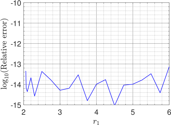
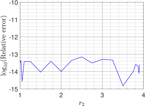
Figure 2: Results for the two confocal ellipses domain: Relative errors in the computed conformal capacity for fixed $r_{2}=2$ (left) and fixed $r_{1}=4$ (right).

3.2 Complete elliptic integrals

We recall the following facts about complete elliptic integrals and hypergeometric functions, needed for the sequel. The Gaussian hypergeometric function is the analytic continuation of the series

$$F(a,b;c;z)={}_{2}F_{1}(a,b;c;z)=\sum_{n=0}^{\infty}\frac{(a,n)(b,n)}{(c,n)}\frac{z^{n}}{n!}\,,\>\>|z|<1\,.$$ (19)

to the slit plane $\mathbb{C}\setminus[1,\infty)$ where $a,b,$ and $c$ are complex numbers with $c\neq 0,-1,-2,\ldots$. Here $(a,n)$ is the Appell symbol or the shifted factorial function

$$(a,n)=a(a+1)(a+2)\cdots(a+n-1)$$

for $n\in\{1,2,3,\ldots\}$ and $(a,0)=1$ for $a\neq 0$. The complete elliptic integrals of the first kind ${K}(r)$ and ${K}^{\prime}(r)$ are defined by

$${K}(r)=\frac{\pi}{2}F(1/2,1/2;1;r^{2}),\qquad{K}^{\prime}(r)={K}(r^{\prime}),\text{ and }r^{\prime}=\sqrt{1-r^{2}}\,,$$ (20)

and the elliptic integrals of the second kind ${E}(r)$ and ${E}^{\prime}(r)$ are defined by

$${E}(r)=\frac{\pi}{2}F(1/2,-1/2;1;r^{2}),\qquad{E}^{\prime}(r)={E}(r^{\prime}),\text{ and }r^{\prime}=\sqrt{1-r^{2}}\,.$$ (21)

Then $K\colon(0,1)\to(\pi/2,\infty)$ is an increasing homeomorphism and $E\colon(0,1)\to(1,\pi/2)$ is a decreasing homeomorphism. The decreasing homeomorphism $\mu\colon(0,1)\to(0,\infty)$ is defined by

$$\mu(r)=\frac{\pi}{2}\,\frac{{K}^{\prime}(r)}{{K}(r)}\,.$$ (22)

The basic properties of these functions can be found in [20, 2, 8, 37]. For example, it follows from [2, (5.2)] for $0<r<1$ that

$$\mu(r)=2\mu\left(\frac{2\sqrt{r}}{1+r}\right)\,,\quad\mu(r)=\frac{1}{2}\mu\left(\frac{1-r^{\prime}}{1+r^{\prime}}\right),\quad\mu(r)\mu(r^{\prime})=\frac{\pi^{2}}{4}.$$ (23)

In the numerical calculations in this paper, we compute the values of $\mu(r)$ through (22) where the values of ${K}(r)$ and ${K}^{\prime}(r)$ are computed by the MATLAB function ellipke. Since $0<r<1$ and $r^{\prime}=\sqrt{1-r^{2}}$, it readily follows that

$$r<\frac{2\sqrt{r}}{1+r}<1\quad{\rm and}\quad 0<\frac{1-r^{\prime}}{1+r^{\prime}}<r.$$

Thus, when $r$ is too close to $0$, we can use the first formula in (23) to get accurate results with MATLAB function ellipke. When $r$ is very close to $1$, we use the second formula in (23).

3.3 Jacobi’s inversion formula for $\mu$

In his fundamental work on elliptic functions, C.G.J. Jacobi proved several dozens of formulas for these functions and related functions such as theta functions. Many of these formulas involved infinite products. As pointed out in [2, Thm 5.24(2)], some of these formulas can be rewritten so as to give formulas for $\mu^{-1}(y)\,.$ We give two examples. Jacobi’s inversion formula for $\mu$ is [2, Thm 5.24(2)]

$$\mu^{-1}(y)^{2}=1-\prod\limits_{n=1}^{\infty}\left(\frac{1-q^{2n-1}}{1+q^{2n-1}}\right)^{8}\,,\,q=\exp(-2y)\,,\,\,y>0\,.$$

Another example of Jacobi’s work is the following formula for $\mu^{-1}(y)$ in terms of theta functions

$$\mu^{-1}(y)=\left(\frac{\theta_{2}(0,q)}{\theta_{3}(0,q)}\right)^{2}\,,\quad q={\rm exp}(-2y)\,\,,y>0\,,$$ (24)

$$\theta_{2}(0,q)=2\sum_{n=0}^{\infty}q^{(n+1/2)^{2}}\,,\quad\theta_{3}(0,q)=1+2\sum_{n=1}^{\infty}q^{n^{2}}\,\,.$$ (25)

Because these theta functions converge very fast in $[0,0.95]\,,$ a few terms of series expansion are enough to achieve numerical values correct up to 15 decimal places. A Newton algorithm for computing $\mu^{-1}(y)$ was implemented in [2, pp. 92, 438].

3.4 Square in square

In our second example, the domain $G$ is the difference of two concentric squares

$$((-2,2)\times(-2,2))\setminus((-2a,2a)\times(-2a,2a))$$

where $0<a<1$. The exact value of the capacity of this domain is [7, pp. 103-104]

$$\mathrm{cap}(G)=\frac{4\pi}{\mu(r)}\,,$$ (26)

where

$$c=\frac{1-a}{1+a},\quad u=\mu^{-1}\left(\frac{\pi c}{2}\right),\quad v=\mu^{-1}\left(\frac{\pi}{2c}\right),\quad r=\left(\frac{u-v}{u+v}\right)^{2}\,.$$

Then, by [2, Exercises 5.8(3)], we have

$$u^{2}+v^{2}=\left(\mu^{-1}\left(\frac{\pi c}{2}\right)\right)^{2}+\left(\mu^{-1}\left(\frac{\pi^{2}/4}{\pi c/2}\right)\right)^{2}=1$$

and hence

$$r=\frac{1-2uv}{1+2uv}\,.$$

By [2, (5.2)], we have

$$\mu(2uv)\mu(r)=\mu(2uv)\mu\left(\frac{1-2uv}{1+2uv}\right)=\frac{\pi^{2}}{2}\,.$$

Thus, it follows from (26) that

$$\mathrm{cap}(G)=\frac{8}{\pi}\mu(2uv)\,,$$ (27)

We use the MATLAB function annq with $\alpha=1+a\in G$, $z_{2}=0$, and $n=2^{17}$ to calculate the capacity for several values of $a$ between $0.1$ and $0.9$. The obtained results are presented in Table 1. Table 1 presents also the exact capacity and the numerical results computed in [17] using an $hp$-FEM algorithm. We see from the results presented in the table that accurate results can be obtained using the presented method. The last column in Table 1 presents the CPU time (in seconds) for our method. The GMRES requires between $23$ to $25$ iterations only to converge. The obtained results using the presented method are not as accurate as the results obtained by the $hp$-FEM algorithm in [17]. This is expected when we compare BIM and FEM for domains with corners.

Table 1: The capacity values for the square in square domain.

$a$	Our Method	[17]	Exact value	Time (sec)
0.1	2.83977741905231	2.83977741905223	2.83977741905224	6.6
0.2	4.13448702423319	4.134487024234081	4.13448702423409	6.5
0.3	5.63282800094106	5.632828000941654	5.63282800094165	6.5
0.4	7.56153153980938	7.5615315398105745	7.56153153981058	7.1
0.5	10.2340925693693	10.23409256936805	10.2340925693681	7.1
0.6	14.2348796758222	14.234879675824363	14.2348796758244	6.6
0.7	20.9015816764098	20.901581676413954	20.901581676414	6.4
0.8	34.2349151987643	34.23491519877346	34.2349151987734	6.9
0.9	74.2349151987441	74.23491519877882	74.2349151987788	6.9

3.5 Polygon in polygon

In the third example, we consider the doubly connected domain $G$ between two polygons. We assume that both polygons have $m$ vertices where $m\geq 3$. We assume that the vertices of the external polygon are the roots of the unity and hence lie on the unit circle $|z|=1$. For the inner polygon, we assume that the vertices are the roots of the unity multiplied by $q=0.5$ and thus lie on the circle $|z|=q$ (see Figure 3 for $m=5$).

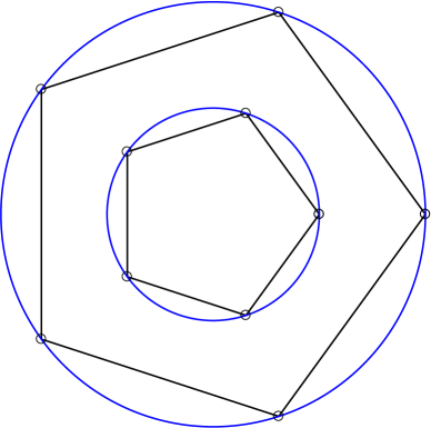
Figure 3: The polygon in polygon domain $G$ for $m=5$ and $q=0.5$. The figure shows also the annulus $q<|z|<1$ where the vertices of the two polygons are on the circles $|z|=1$ and $|z|=q$.

The exact value of capacity of the domain is unknown (except for $m=4$ where the capacity can be computed as in the square in square example, which for $q=0.5$, is $10.2340925693681$). We use the MATLAB function annq with $\alpha=(1+q)/2\in G$, $z_{2}=0$, and $n=40320$ to calculate the capacity for several values of $m$. The computed capacity is presented in Table 2. As we can see from the table, as $m$ increases, the capacity approaches the capacity of the annulus $q<|z|<1$ which is $2\pi/\log(1/q)$. For $q=0.5$, the capacity of the annulus is $9.064720283654388$. For some values of $m$, Table 2 presents also approximate values of the capacity from [5]. The last column in Table 2 presents the CPU time (in seconds) for our method.

Table 2: The capacity values for the polygon in polygon domain.

$m$	Our Method	[5]	Time (sec)
3	12.4411574383	12.4412	4.0
4	10.2340925693267		2.5
5	9.62720096044514	9.6266	2.6
7	9.25977557690559	9.2598	2.4
9	9.15441235751744	9.1541	2.1
15	9.08360686195382		1.8
30	9.06705650051687		1.5

4 Complement of two slits

In this section, we consider a doubly connected domain $\Omega$ whose complementary components are the two non-intersecting segments $E=[a,b]$ and $F=[c,d]$ where $a$, $b$, $c$ and $d$ are complex numbers (see Figure 4 (left) for $a=0$, $b=1$, $c=1-\mathrm{i}$ and $d=3+2\mathrm{i}$). Computing the capacity of such domain $\Omega$ has been considered recently in [9] using Weierstrass elliptic functions. Here, we shall compute the capacity of $\Omega$ using the method presented in Section 2. However, a direct application of the method presented in Section 2 is not possible since the boundaries of $\Omega$ are not Jordan curves. So, we need to first map the given domain $\Omega$ onto a domain $G$ of the form considered in Section 2. Up to the best of our knowledge, there is no analytic formula for a conformal mapping from the above doubly connected domain $\Omega$ onto a doubly connected domain $G$ bordered by smooth Jordan curves. So, we need to use numerical methods to find such an equivalent domain $G$. Such a conformally equivalent domain $G$ can be computed using the iterative method presented recently in [33]. The computed domain $G$ will be bordered by ellipses as in Figure 4 (right). We refer the reader to [33] for details on this iterative numerical method. The MATLAB function annq with $n=2^{11}$ is then used to compute the capacity of $G$, and hence the capacity of $\Omega$, for several values of $a$, $b$, $c$ and $d$, as in the following examples.

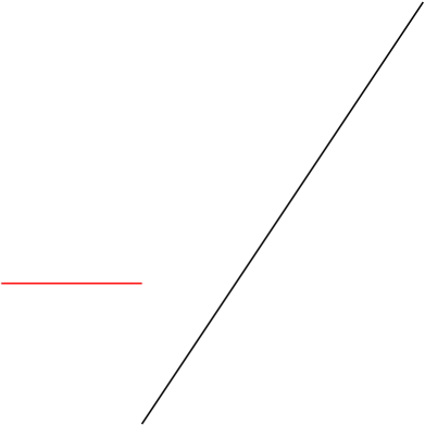
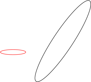
Figure 4: The two segments domain $\Omega$ for $a=0$, $b=1$, $c=1-\mathrm{i}$ and $d=3+2\mathrm{i}$ (left) and the preimage domain $G$ bordered by ellipses (right).

4.1 Two segments on the real axis

When $E=[0,1]$ and $F=[c,d]$ with $d>c>1$, the exact capacity of $\Omega$ is known and is given by [44, 5.54 (1), 5.60(1)]

$$\frac{\pi}{\mu\left(\sqrt{\frac{d-c}{c(d-1)}}\right)}\,.$$ (28)

We tested our methods for several values of $c$ and $d$. First, we fixed $c=2$ and chose $d$ between $2.1$ and $10$. Then we fixed $c=d-1$ and chose $d$ between $2.1$ and $10$. For this case, the relative errors in the computed values are presented in Figure 5. As we can see from Figure 5, the presented method gives accurate results with relative error around $10^{-14}$. Table 3 presents the approximate values of the capacity, the exact values of the capacity, and the total CPU time for several values of $c$ and $d$.

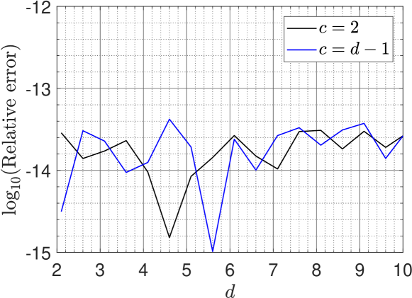
Figure 5: Relative errors of the computed conformal capacity for ring domains with complementary components $[0,1]$ and $[c,d]\,,$ $2.1\leq d\leq 10$.

Table 3: The values of $\mathrm{cap}([0,1],[c,d])$.

$c$	$d$	Computed value	Exact value	Relative Error	Time (sec)
$1.1$	$2$	$2.78768694945386$	$2.7876869494539$	$1.3\times 10^{-14}$	3.8
$1.1$	$5$	$3.11161184032646$	$3.11161184032641$	$1.7\times 10^{-14}$	7.0
$1.1$	$10$	$3.19100134481022$	$3.19100134481039$	$5.2\times 10^{-14}$	10.0
$2$	$3$	$1.56340192269607$	$1.56340192269611$	$2.7\times 10^{-14}$	1.7
$2$	$5$	$1.78056882835563$	$1.78056882835559$	$1.8\times 10^{-14}$	2.5
$2$	$10$	$1.9006702400055$	$1.90067024000545$	$2.5\times 10^{-14}$	2.9

4.2 Two vertical segments

The case $E=[a,\overline{a}]$ and $F=[c,\overline{c}]$, with ${\rm Im}\,a\neq 0$ and ${\rm Im}\,c\neq 0$, has been considered in [6, Figure E]. We use our method to calculate the capacity for the same values of $a$ and $c$ that considered in [6, Table 3]. A comparison of the results computed using our method vs the method presented in [6] is given in Table 4 where the last column presents the CPU time for our method.

Table 4: The values of $\mathrm{cap}([a,\overline{a}],[c,\overline{c}])$.

$a$	$c$	Our Method	[6]	Time (sec)
$0+\mathrm{i}$	$5+2\mathrm{i}$	1.569943666568835	1.56994325474948999	3.2
$0+2\mathrm{i}$	$5+2\mathrm{i}$	1.873067768653831	1.87306699654806386	2.9
$0+3\mathrm{i}$	$5+2\mathrm{i}$	2.082038279851203	2.08203777712328096	3.8
$0+4\mathrm{i}$	$5+2\mathrm{i}$	2.232598863252026	2.23259828277206300	4.5
$0+5\mathrm{i}$	$5+2\mathrm{i}$	2.341589037102932	2.34158897620030515	5.0
$0+3\mathrm{i}$	$5+3\mathrm{i}$	2.352412309035929	2.35241226225174034	3.7

4.3 Two general segments

Finally, let

$$f(a,b,c,d)=\mathrm{cap}([a,b],[c,d]),$$

where $a$, $b$, $c$, and $d$ are complex numbers. We fix $a=0$ and $b=4$. Then, for a given point $z_{1}$ in the simply connected domain $\hat{\Omega}$ exterior to $[a,b]$, we define the function $u(x,y)$ by

$$u(x,y)=f([0,4],[z_{1},x+\mathrm{i}y])=\mathrm{cap}([0,4],[z_{1},x+\mathrm{i}y])\,.$$

for $0<x<12$ and $0<y<10$ such that the segment $[z_{1},x+\mathrm{i}y]$ is in $\hat{\Omega}$ with $x+\mathrm{i}y\neq z_{1}$. We plot the contour lines for the function $u(x,y)$ corresponding to several levels. The contour lines for $z_{1}=6+2\mathrm{i}$ and $z_{1}=6+6\mathrm{i}$ are shown in Figure 6. Table 5 presents the approximate values of $\mathrm{cap}([0,4],[z_{1},z_{2}])$ for several values of $z_{1}$ and $z_{2}$.

If the interval $[a,b]=[0,1]$ is considered instead of $[a,b]=[0,4]$, we obtain the results shown in Figure 7 for $z_{1}=6+4\mathrm{i}$ and $z_{1}=5+4\mathrm{i}$.

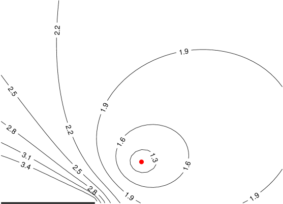
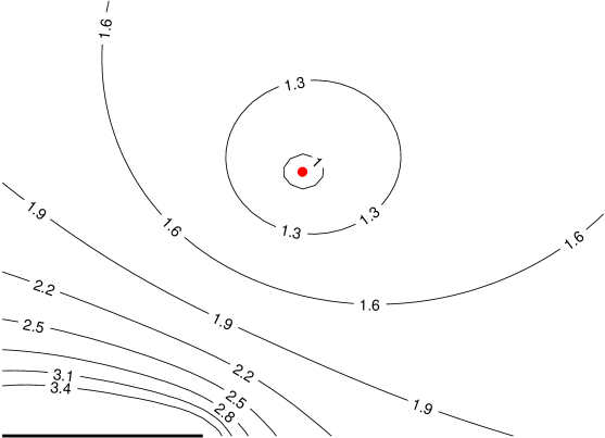
Figure 6: Results for the two segments domain: the contour lines of the function $u(x,y)=\mathrm{cap}([0,4],[6+2\mathrm{i},x+\mathrm{i}y])$ (left) and $u(x,y)=\mathrm{cap}([0,4],[6+6\mathrm{i},x+\mathrm{i}y])$ (right).

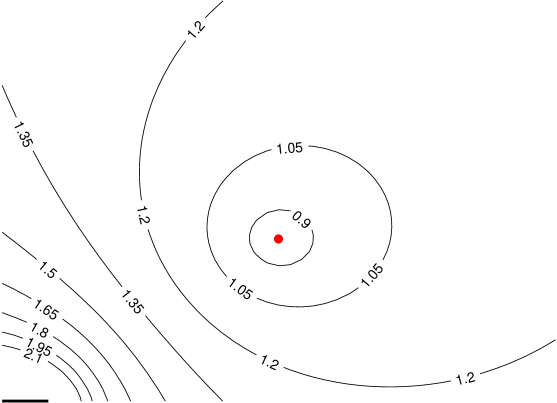
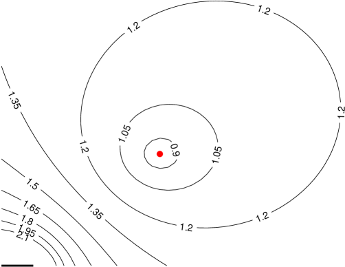
Figure 7: Results for the two segments domain: the contour lines of the function $u(x,y)=\mathrm{cap}([0,1],[6+4\mathrm{i},x+\mathrm{i}y])$ (left) and $u(x,y)=\mathrm{cap}([0,1],[5+4\mathrm{i},x+\mathrm{i}y])$ (right).

Table 5: The values of $\mathrm{cap}([0,4],[z_{1},z_{2}])$.

$z_{2}\backslash z_{1}$	$6+2\mathrm{i}$	$6+4\mathrm{i}$	$6+6\mathrm{i}$
$1+\mathrm{i}$	4.437462457504561	3.780635179650131	3.564215562104226
$1+2\mathrm{i}$	3.317286587467568	2.860692915566007	2.711077789477010
$1+3\mathrm{i}$	2.846059598705353	2.436675855049381	2.295322432200487
$1+4\mathrm{i}$	2.604420470210280	2.202349785968325	2.046526840859631
$1+5\mathrm{i}$	2.470153941168786	2.066569200937597	1.886514461888595

5 Rings with a segment as a boundary component

In this section, we compute the capacity of doubly connected domains $\Omega$ whose boundary components are a slit and a piecewise smooth Jordan curve. Such domains cannot be mapped directly onto an annulus using the method presented in Section 2. To use the method presented in Section 2, we shall use first elementary mappings to map the domain $\Omega$ onto a domain $G$ of the types considered in Section 2. Then the domain $G$ is mapped onto an annulus $R=\{z\in\mathbb{C}\;:\;q<|z|<1\}$ and hence the capacity of $\Omega$ is $2\pi/\log(1/q)$. In this subsection we consider two examples where the exact value of the capacity for the first example is known.

5.1 Segment and circle

First, we consider the doubly connected domain $\Omega$ in the exterior of the segment $[0,1]$ and the circle $|z-a|=r$ where $a$ is a real number with $a>1+r>1$ (see Figure 8 (left) for $r=0.9$ and $a=2$). The exact conformal capacity for this domain $\Omega$ is known and given by [44, 5.54(2)]

$$\mathrm{cap}(\Omega)=\frac{2\pi}{\mu(\tau)},\quad\tau=\frac{r}{a^{2}-a-r^{2}}\,,$$ (29)

where $\mu$ is given by (22).

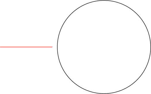
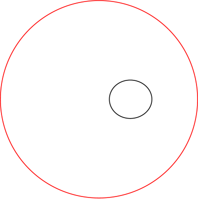
Figure 8: The segment and circle domain $\Omega$ for $a=2$ and $r=0.9$ (left); and the image of this unbounded domain under the mapping $\zeta=\Psi^{-1}(z)$ (right).

To apply our method presented in Section 2, we shall use first elementary mappings to map the domain $\Omega$ onto a domain $G$ of the types considered in Section 2. It is known that the function

$$z=\Psi(\zeta)=\frac{1}{4}\left(\zeta+\frac{1}{\zeta}\right)+\frac{1}{2}$$

maps conformally the interior of the unit circle $|\zeta|=1$ onto the exterior of the segment $[0,1]$. Hence, its inverse function is given by

$$\zeta=\Psi^{-1}(z)=\frac{1}{(2z-1)\left(1+\sqrt{1-\frac{1}{(2z-1)^{2}}}\right)},$$ (30)

where we choose the branch for which $\sqrt{1}=1$. The function $\zeta=\Psi^{-1}(z)$ maps the segment $[0,1]$ onto the unit circle $|\zeta|=1$ and the exterior of the segment $[0,1]$ onto the interior of the unit circle $|\zeta|=1$. The function $\zeta=\Psi^{-1}(z)$ maps also the circle $|z-a|=r$ in the $z$-plane onto a smooth Jordan curve inside the unit circle $|\zeta|=1$. Consequently, the function $\zeta=\Psi^{-1}(z)$ maps the doubly connected domain $\Omega$ onto a bounded doubly connected domain $G$ of the form considered in Section 2 (see Figure 8 (right)).

Then we use the MATLAB function annq with $n=2^{11}$ to calculate approximate values for the capacity of $G$, and hence the capacity of $\Omega$, for several values of $a$ and $r$. First, we fixed $r=1$ and chose values of $a$ between $2.05$ and $6$. Then, we fixed $a=4$ and chose values of $r$ between $0.05$ and $2.95$. Figure 9 presents the relative errors in the calculated values. The exact values and the computed approximate values of the capacity are presented in Table 7 for several values of $r$ and $a$.

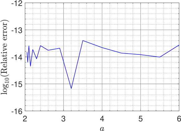
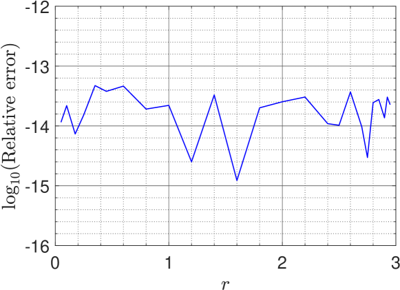
Figure 9: Results for the segment and circle domain: Relative errors of the computed conformal capacity for fixed $r=1$ (left) and fixed $a=4$ (right).

Table 6: The capacity values for the segment and circle domain.

$r$	$a$	Computed value	Exact value	Relative Error	Time (sec)
$0.1$	$1.2$	$2.89834979084902$	$2.89834979084894$	$2.7\times 10^{-14}$	0.17
$0.1$	$2.2$	$1.3496258349391$	$1.34962583493908$	$1.6\times 10^{-14}$	0.15
$0.1$	$5.2$	$0.927796431822476$	$0.927796431822507$	$3.3\times 10^{-14}$	0.17
$1.0$	$2.1$	$4.31652297947248$	$4.31652297947259$	$2.6\times 10^{-14}$	0.19
$3.0$	$4.1$	$4.6213142805315$	$4.62131428053158$	$1.8\times 10^{-14}$	0.18
$5.0$	$6.1$	$4.69478341049729$	$4.69478341049717$	$2.5\times 10^{-14}$	0.19

5.2 Segment and ellipse

In connection with the examples presented in Subsections 4.1 and 5.1, we consider the following example to show how the capacity of the domains changes when the geometry of the domains changes. Let $G_{r}$ be the doubly connected domain whose complementary components are the two non-intersecting closed sets $E=[0,1]$ and $F_{r}$ where $F_{r}$ is the closed set of points in the interior and on the boundary of the ellipse

$$\eta_{r}(t)=a+b\cos(t)-\mathrm{i}r\sin(t),\quad 0\leq t\leq 2\pi,$$

where

$$a=\frac{1}{2}(d+c),\quad b=\frac{1}{2}(d-c),\quad 0<r\leq b<a,$$

and $1<c<d$ (see Figure 10 (center)).

For $r=0$, $F_{r}$ reduced to the segment $F_{0}=[c,d]$ and hence $G_{0}$ is the doubly connected domain exterior to the two segments $E=[0,1]$ and $F_{0}=[c,d]$ as considered in Subsection 4.1 (see Figure 10 (left)). The exact value of $\mathrm{cap}(E,F_{0})$ is given by (28), i.e.,

$$\mathrm{cap}(E,F_{0})=\frac{\pi}{\mu\left(s\right)}\,,\qquad s=\sqrt{\frac{d-c}{c(d-1)}},$$ (31)

where $\mu$ is given by (22). When $r=b$, $F_{b}$ is the closed disk $|z-a|\leq b$ and the domain $G_{b}$ is then the doubly connected domain exterior to the segment $E=[0,1]$ and the closed disk $F_{b}=\{x\,|\,|z-a|\leq b\}$ which was considered in Subsection 5.1 (see Figure 10 (right)). The exact value of $\mathrm{cap}(E,F_{b})$ is given by (29), i.e.,

$$\mathrm{cap}(E,F_{b})=\frac{2\pi}{\mu(s)}\,,\quad s=\frac{b}{a^{2}-a-b^{2}}\,.$$ (32)

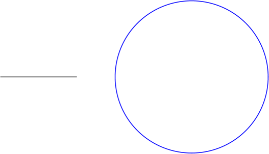
Figure 10: The domain $G_{r}$ with $c=1.5$, $d=3.5$ for $r=0$ (left), $r=0.1$ (center) and $r=b$ (right).

It is clear from the definition of the closed set $F_{r}$ that $F_{0}\subseteq F_{r}\subseteq F_{b}$ for $0\leq r\leq b$. As $r$ changes continuously from $0$ to $b$, the closed set $F_{r}$ changes continuously from the segment $F_{0}$ to the disk $F_{b}$. Here, we shall compute the exact value of the capacity $\mathrm{cap}(E,F_{r})$ and show that $\mathrm{cap}(E,F_{r})$ will change from $\mathrm{cap}(E,F_{0})$ to $\mathrm{cap}(E,F_{b})$ as $r$ changes from $0$ to $b$.

By the elementary mapping

$$\zeta=\Psi_{1}(z)=\frac{z-a}{b},$$

the unbounded domain $G$ is mapped conformally onto the unbounded domain $G_{1}$ exterior to the segment $[-a/b,-(a-1)/b]$ and the ellipse

$$\eta_{1}(t)=\cos(t)-\mathrm{i}(r/b)\sin(t),\quad 0\leq t\leq 2\pi.$$

We can easily show that the function

$$\zeta=\Psi_{2}(\xi)=\xi+\frac{1-(r/b)^{2}}{4}\frac{1}{\xi}$$

maps the domain exterior to the circle $|\xi|=(1+r/b)/2$ onto the domain exterior of the ellipse. Hence, the inverse mapping

$$\xi=\Psi^{-1}_{2}(\zeta)=\zeta\left(\frac{1}{2}+\frac{1}{2}\sqrt{1-\frac{1-(r/b)^{2}}{\zeta^{2}}}\right),$$

maps the domain $G_{1}$ onto the domain $G_{2}$ exterior to the circle $|\xi|=(1+r/b)/2$ and the segment $[c_{1},d_{1}]$ where

$$c_{1}=-\frac{a+\sqrt{a^{2}-b^{2}+r^{2}}}{2b},\quad d_{1}=-\frac{a-1+\sqrt{(a-1)^{2}-b^{2}+r^{2}}}{2b},$$ (33)

and the branch of the square root is chosen such that $\sqrt{1}=1$. Finally, the function

$$w=\Psi_{3}(\xi)=\frac{\xi-c_{1}}{d_{1}-c_{1}},$$

maps the domain $G_{2}$ onto the domain $G_{3}$ exterior to the circle $|w-\hat{a}|=\hat{r}$ and the segment $[0,1]$ where

$$\hat{a}=-\frac{c_{1}}{d_{1}-c_{1}},\quad\hat{r}=\frac{b+r}{2b}\frac{1}{d_{1}-c_{1}}.$$ (34)

Hence, the analytic value of $\mathrm{cap}(E,F_{r})$ can be obtained since the exact value of conformal capacity of the domain $G_{3}$ is known [44, 5.54(2)],

$$\mathrm{cap}(E,F_{r})=\frac{2\pi}{\mu(\tau_{r})}$$ (35)

where

$$\tau_{r}=\frac{\hat{r}}{\hat{a}^{2}-\hat{a}-\hat{r}^{2}}\,.$$ (36)

The value of $\tau_{r}$ can be obtained in terms of $c$, $d$ and $r$ as following

$$\tau_{r}=\frac{2(d-c+2r)\left(1+\sqrt{dc+r^{2}}-\sqrt{dc-d-c+1+r^{2}}\right)}{\left(d+c+2\sqrt{dc+r^{2}}\right)\left(d+c-2+2\sqrt{dc-d-c+1+r^{2}}\right)-(d-c+2r)^{2}}.$$

For $r=0$, the capacity given by (35) becomes

$$\frac{2\pi}{\mu(\tau_{0})}$$ (37)

where

$$\tau_{0} = \frac{2(d-c)\left(1+\sqrt{dc}-\sqrt{dc-d-c+1}\right)}{\left(d+c+2\sqrt{dc}\right)\left(d+c-2+2\sqrt{dc-d-c+1}\right)-(d-c)^{2}}$$ (38)

$$= \frac{\sqrt{d}-\sqrt{c}}{\sqrt{d}+\sqrt{c}}\,\frac{\sqrt{cd}-\sqrt{(c-1)(d-1)}+1}{\sqrt{cd}+\sqrt{(c-1)(d-1)}-1}$$

After tedious algebra, we find that $s$ in (31) is related to $\tau_{0}$ in (38) through

$$s=\frac{2\sqrt{\tau_{0}}}{1+\tau_{0}},$$ (39)

which, in view of (23), implies that $\mu(\tau_{0})=2\mu(s)$. Hence,

$$\mathrm{cap}(E,F_{0})=\frac{\pi}{\mu(s)}=\frac{2\pi}{\mu(\tau_{0})}$$

and thus the capacity $\mathrm{cap}(E,F_{r})$ given by (35) reduced to the capacity $\mathrm{cap}(E,F_{0})$ for $r=0$. Furthermore, when $r=b$, then it follows from (33) and (34) that $\hat{a}=a$ and $\hat{r}=r=b$. Hence, it follows from (36) that

$$\tau_{b}=\frac{r}{a^{2}-a-r^{2}}\,,$$

which implies that the capacity $\mathrm{cap}(E,F_{r})$ given by (35) reduced to the Formula (32) for $r=b$.

The values of $\mathrm{cap}(E,F_{r})$ for $c=1.5$, $d=3.5$, $0\leq r\leq b$ (where $b=(d-c)/2=1$) is given in Figure 11. As we can see from Figure 11, the capacity $\mathrm{cap}(E,F_{r})$ changes continuously and rapidly increases from $\mathrm{cap}(E,F_{0})$ to $\mathrm{cap}(E,F_{b})$ as $r$ changes continuously from $0$ to $b$.

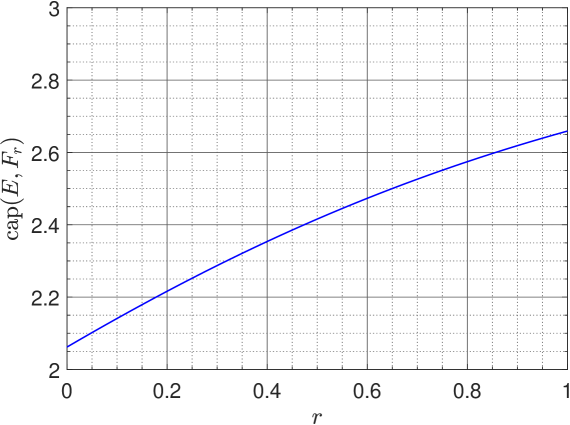
Figure 11: The values of $\mathrm{cap}(E,F_{r})$ for $c=1.5$, $d=3.5$, $0\leq r\leq b$.

5.3 Segment and polygon

In this example, we consider the doubly connected domain $\Omega$ in the exterior of the segment $[0,1]$ and a polygon with $m$ vertices where $m\geq 3$. We assume that the vertices of the polygon are given by

$$v_{k}=a-re^{\frac{-2k\pi\mathrm{i}}{m}},\quad k=0,1,2,\ldots,m-1$$

(see Figure 12 (left) for $a=1.6$, $r=0.5$, and $m=3$). For this example, the exact value of the conformal capacity is unknown. To use the method described in Section 2, we first use the mapping function $\zeta=\Psi^{-1}(z)$ in Subsection 5.1 to map the doubly connected domain $\Omega$ onto a bounded doubly connected domain $G$ of the form we considered in Section 2 (see Figure 12 (right)). Then, for the new domain $G$, the MATLAB function annq is used with $n=15\times 2^{9}$ to calculate approximate values for the capacity of $\Omega$ for several values of $m$, $a$ and $r$. First, we fixed $r=1$ and chose values of $a$ between $2.05$ and $6$. The computed capacity for $m=3,4,8,16$ are presented in Figure 13 (left). Then, we fixed $a=4$ and chose values of $r$ between $0.05$ and $2.95$. The computed capacity for $m=3,4,8,16$ are presented in Figure 13 (right). Figure 13 presents also the capacity for the segment with circle domain in the previous examples for the same values of $a$ and $r$. Table 7 presents the calculated values of the capacity for the segment with circle domain and for the segment with polygon domain for several values of $a$, $r$, and $m$. As we can see from the results presented in the table, the capacity of the segment and polygon domain approaches the the capacity of the segment and circle domain as the number of vertices $m$ increases.

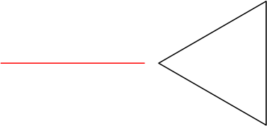
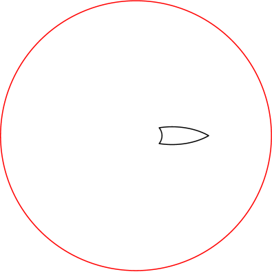
Figure 12: The segment and polygon domain $\Omega$ for $a=1.6$ and $r=0.5$ (left); and the image of this unbounded domain under the mapping $\zeta=\Psi^{-1}(z)$ (right).

Table 7: The capacity values for the segment with polygon domain.

$r$	$a$	$m$	Capacity (segment and polygon)	Capacity (segment and circle)
$1$	$2.1$	$3$	$3.385465691885468$	$4.31652297947259$
		$8$	$3.996010644504850$
		$16$	$4.198837938505387$
		$128$	$4.314154067689326$
$0.5$	$4$	$3$	$1.291427925789600$	$1.38309579015095$
		$8$	$1.368162812590014$
		$16$	$1.379193284259540$
		$128$	$1.383032359435526$
$2.5$	$10$	$3$	$1.199970598794575$	$1.28290663972126$
		$8$	$1.268817744415183$
		$16$	$1.279211726247828$
		$128$	$1.282846509334037$

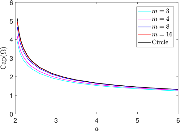
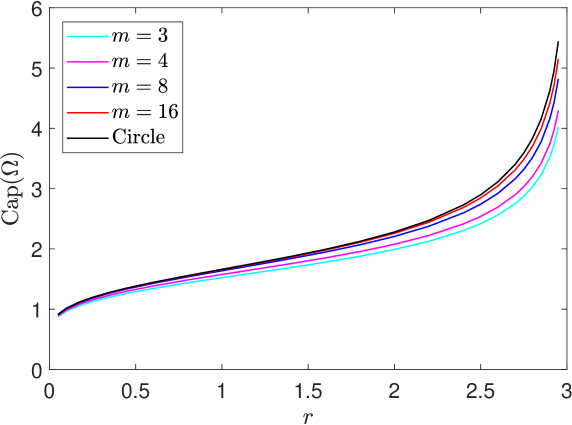
Figure 13: Results for the segment and polygon domain: The computed conformal capacity for fixed $r=1$ (left) and fixed $a=4$ (right).

6 The upper half-plane with a slit

In this section, we consider the doubly connected domain $\Omega=\mathbb{H}^{2}\setminus[a,b]$ where $\mathbb{H}^{2}$ is the upper half-plane $\{z\in\mathbb{C}:{\rm Im}\,(z)>0\}$ and, $a$ and $b$ are two complex numbers in $\mathbb{H}^{2}$ (see Figure 14 (left)). For such domains $\Omega$, we cannot directly apply the method described in Section 2. So, we first map the domain $\Omega$ onto a domain $G$ of the forms considered in Section 2. Since there is no exact conformal mapping from a domain such as $\Omega$ onto a doubly connected domain $G$ bordered by smooth Jordan curves, we find such an equivalent domain $G$ using numerical methods. In this paper, we compute such a domain $G$ using the iterative numerical method presented in [33] (see Figure 14). We will omit the details here about the iterative method and refer the reader to [33]. Then, we compute the capacity of the the given domain $\Omega$ by applying the MATLAB function annq with $n=2^{11}$ to the new domain $G$.

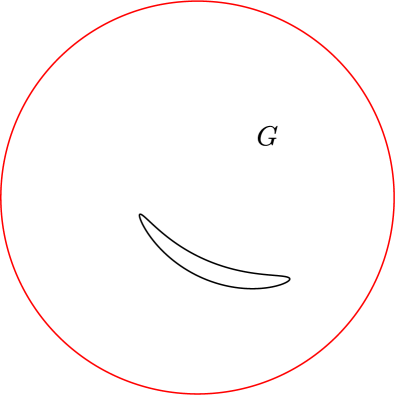
Figure 14: The half-plane with a segment domain $\Omega$ for $a=1+0.5\mathrm{i}$ and $b=-1+1.5\mathrm{i}$ (left) and the preimage domain $G$ bordered by smooth Jordan curves (right).

For the segment $F=[s\mathrm{i},r\mathrm{i}]$ where $r>s>0$ are real numbers, the exact capacity of $\Omega$ is known and is given by [44, (5.56), Theorem 8.6 (1)]

$$\frac{2\pi}{\mu\left(\tanh\left(\frac{1}{2}\log\frac{r}{s}\right)\right)}\,.$$ (40)

We tested our methods for several values of $s$ and $r$. First, we chose the vertical segment $F=[s\mathrm{i},(1+s)\mathrm{i}]$, i.e., $a=s\mathrm{i}$ and $b=(1+s)\mathrm{i}$, for $0.05\leq s\leq 6$. For this case, the relative errors in the calculated values of the capacity are presented in Figure 15 (left). We see from Figure 15 (left) that the proposed method gives accurate results with relative error around $10^{-14}$. The calculated and the exact values of the capacity as well as the total CPU time for several values of $s$ and $r$ are presented in Table 8.

Table 8: The values of $\mathrm{cap}(\Omega)$ for $\Omega=\mathbb{H}^{2}\setminus[s\mathrm{i},r\mathrm{i}]$.

$s$	$r$	Computed value	Exact value	Relative Error	Time (sec)
$0.1$	$1$	$4.69363108974789$	$4.6936310897475$	$8.2\times 10^{-14}$	2.9
$0.1$	$5$	$6.74589984699685$	$6.74589984699653$	$4.8\times 10^{-14}$	5.3
$0.1$	$10$	$7.62853775997519$	$7.62853775997481$	$5.0\times 10^{-14}$	6.6
$1$	$2$	$2.55852314234207$	$2.55852314234201$	$2.1\times 10^{-14}$	2.2
$1$	$5$	$3.80134048001095$	$3.80134048001091$	$1.7\times 10^{-14}$	2.6
$1$	$10$	$4.6936310897476$	$4.6936310897475$	$2.1\times 10^{-14}$	3.1

We also compute the values of the capacity for the vertical segment $F=[(3-s)\mathrm{i},(3+s)\mathrm{i}]$ for $0.05\leq s\leq 2.95$ and for the horizontal segment $F=[-s+3\mathrm{i},s+3\mathrm{i}]$ for $0.05\leq s\leq 3$. Both segments pass through the point $3\mathrm{i}$ and have the length $2s$. The results are presented in Figure 15 (right). Figure 15 (right) shows that the capacity increases as the length of the segment increases. For vertical segment, the capacity increases more rapidly when the segment becomes close to the real line.

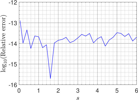
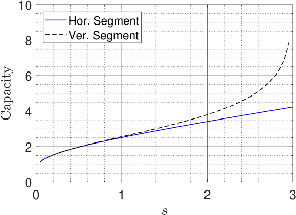
Figure 15: Results for the half-plane with a segment domain: Relative errors of the computed conformal capacity for the segment $F=[s\mathrm{i},(1+s)\mathrm{i}]$ for $0.05\leq s\leq 6$ (left) and the computed capacities (right).

Finally, for a given point $z_{1}$ in $\mathbb{H}^{2}$, we define the function $u(x,y)$ by

$$u(x,y)=\mathrm{cap}(\mathbb{H}^{2}\backslash[z_{1},x+\mathrm{i}y])$$

for $-3<x<3$ and $0<y<3$ such that $x+\mathrm{i}y\neq z_{1}$. We plot the contour lines for the function $u(x,y)$ corresponding to several levels. The contour lines are shown in Figure 16 for $z_{1}=\mathrm{i}$ and $z_{1}=2\mathrm{i}$.

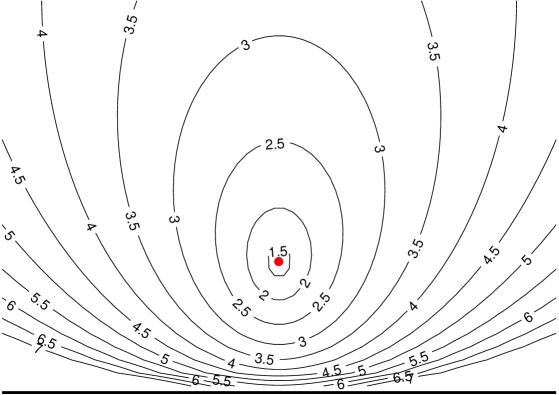
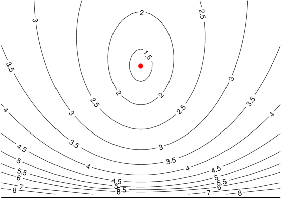
Figure 16: Results for the half-plane with a segment domain: the contour lines of the function $u(x,y)=\mathrm{cap}(\mathbb{H}^{2}\backslash[\mathrm{i},x+\mathrm{i}y])$ (left) and $u(x,y)=\mathrm{cap}(\mathbb{H}^{2}\backslash[2\mathrm{i},x+\mathrm{i}y])$ (right).

7 Domains exterior to thin rectangles

7.1 Two rectangles

We consider in this section the doubly connected domain $G$ exterior to the rectangular closed sets

$$[0,1]\times[0.5-d,0.5+d]\quad{\rm and}\quad[0,1]\times[-0.5-d,-0.5+d]$$

where $0<d<0.5$ (see the Figure 17). We use the MATLAB function annq presented in Subsection 2.6 with $n=2^{15}$ to compute the capacity of $G$ for several values of $d$. When $d=0$, the two rectangles reduced to the two slits $[\mathrm{i}/2,1+\mathrm{i}/2]$ and $[-\mathrm{i}/2,1-\mathrm{i}/2]$. For these two slits, we can use the numerical method presented in Section 4 to compute the capacity of the domain in the exterior to these two slits. The obtained results are presented at the bottom of Table 9.

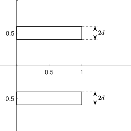
Figure 17: The domain $G$ in the exterior of the rectangular closed sets for $d=0.1$.

Table 9: The capacity values for the domain exterior to the two rectangles.

$d$	Capacity	Time (sec)
0.4	7.55672805385065	2.1
0.3	4.55284511607753	2.1
0.2	3.3856923786737	2.0
0.1	2.68688786213937	2.0
0.05	2.40554719800866	2.1
0.02	2.24063059387802	2.4
0.01	2.18262548680027	2.8
0.005	2.15161636330889	4.9
0	2.11577897412447	25.0

Let $R_{1}$ be the unbounded doubly connected domain exterior to the two slits $[\mathrm{i}/2,1+\mathrm{i}/2]$ and $[-\mathrm{i}/2,1-\mathrm{i}/2]$ (corresponding to $d=0$). The exact value of the capacity of $R_{1}$ can be computed. For $0<k<1$, consider the unbounded doubly connected domain $R_{2}$ exterior to the two slits $[-1/k,-1]$ and $[1,1/k]$. Then the Möbius transform

$$\Psi(z)=\frac{2k}{k-1}\frac{z+1}{kz-1}$$

maps the domain $R_{2}$ onto the unbounded doubly connected domain $R_{3}$ exterior to the two slits $[-1,0]$ and $[s,+\infty]$ where $s=\Psi(1)=4k/(1-k)^{2}$. Thus, the capacity of the domain $R_{2}$ equals to the capacity of $R_{3}$ which can be expressed by [44, 5.60 (1)]

$$\mathrm{cap}(R_{2})=\frac{\pi}{\mu(1/\sqrt{1+s})},\quad s=\frac{4k}{(1-k)^{2}}.$$ (41)

Here $\mu$ is the function defined in (22).

By [8, 119.03], the domain $R_{2}$ can be mapped conformally also onto the unbounded doubly connected domain $R_{4}$ exterior to the two slits $[-t/2-\mathrm{i}b/2,-t/2+\mathrm{i}b/2]$ and $[t/2-\mathrm{i}b/2,t/2+\mathrm{i}b/2]$ with

$$t=\frac{2}{k}\left(E(k)-(1-k^{2}a^{2})K(k)\right),\quad b=\frac{2}{k}\left(E(k^{\prime}_{1},k^{\prime})-k^{2}a^{2}F(k^{\prime}_{1},k^{\prime}))\right)$$

where the functions $E(k),K(k)$ are defined in (21) and (20), resp., and

$$F(z,k)=\int_{0}^{z}\frac{dw}{\sqrt{(1-w^{2})(1-k^{2}w^{2})}},\quad E(z,k)=\int_{0}^{z}\sqrt{\frac{1-k^{2}w^{2}}{1-w^{2}}}dw,$$

and

$$k^{\prime}=\sqrt{1-k^{2}},\quad a=\frac{E(k^{\prime})}{k^{2}K(k^{\prime})}\quad k_{1}=\frac{k}{k^{\prime}}\sqrt{a^{2}-1},\quad k^{\prime}_{1}=\sqrt{1-k_{1}^{2}}.$$

Hence $\mathrm{cap}(R_{4})=\mathrm{cap}(R_{2})$. Further, it is clear that the domain $R_{1}$ can be conformally mapped by the function $\hat{\Psi}(z)=\mathrm{i}(z-1/2)$ onto the domain $R_{4}$ if we choose $k$ such that $t=b=1$. Thus, the exact capacity of $R_{1}$ is given by

$$\mathrm{cap}(R_{1})=\frac{\pi}{\mu(1/\sqrt{1+s})},\quad s=\frac{4k}{(1-k)^{2}}$$ (42)

where $k$ satisfies the equations

$$1=\frac{2}{k}\left(E(k)-(1-k^{2}a^{2})K(k)\right),\quad 1=\frac{2}{k}\left(E(k^{\prime}_{1},k^{\prime})-k^{2}a^{2}F(k^{\prime}_{1},k^{\prime}))\right).$$ (43)

The equations (43) are solved using Mathematica for $k$ and the value of the capacity of $R_{1}$ computed through (42) is $2.1157789709245134$. This value agrees with the value presented at the bottom of Table 9 with relative error $1.5\times 10^{-9}$.

7.2 A vertical rectangle in the upper half-plane

Consider the doubly connected domain $G$ exterior to the rectangular closed set

$$[0.5-d,0.5+d]\times[1,2]$$

in the upper half-plane where $0<d<0.5$ (see the Figure 18 for $d=0.1$). The auxiliary map

$$w=\Psi(z)=\frac{\mathrm{i}z+1}{z+\mathrm{i}}$$ (44)

is used to transform the domain $G$ onto a domain $\hat{G}$ interior to the unit disk and exterior to the piecewise smooth Jordan curve $L$ which is the image of the rectangle under the map $\Psi$. Then $G$ and $\hat{G}$ have the same capacities. We use the function annq with $n=2^{15}$ to compute the capacity of $\hat{G}$ for several values of $d$. When $d=0$, the rectangle reduced to the slit $[\mathrm{i},2\mathrm{i}]$. For the upper half-plane with the slit $[\mathrm{i},2\mathrm{i}]$, we can use the numerical method presented in Section 6 to compute the capacity of the domain exterior to this slit in the upper half-plane. The results are presented in Table 10. The exact value of the capacity of the domain exterior to slit $[\mathrm{i},2\mathrm{i}]$ in the upper half-plane can be computed from (40) and is equal to $2\pi/\mu(1/3)=2.55852314234201$. The result presented at the bottom of Table 10 agrees with the exact value with relative error $4.7\times 10^{-13}$.

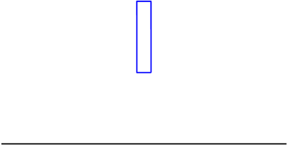
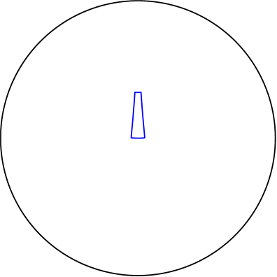
Figure 18: The domain $G$ in the exterior of a vertical rectangular closed set in the upper half-plane (left) and its image $\hat{G}$ under the auxiliary map $\Psi$ (right) for $d=0.1$.

Table 10: The capacity values for the domain exterior to a vertical rectangle in the upper half-plane.

$d$	$\mathrm{cap}(G)$	Time (sec)
0.4	3.71752232703208	2.4
0.3	3.46693660197964	2.2
0.2	3.20488821317939	2.2
0.1	2.9209225535743	2.3
0.05	2.76128813737089	2.6
0.02	2.65173985860514	3.0
0.01	2.60986001541974	3.9
0.005	2.58658944233183	5.4
0	2.55852314234082	16.4

7.3 A horizontal rectangle in the upper half-plane

Consider the doubly connected domain $G$ exterior to the rectangular closed set

$$[0,1]\times[0.5-d,0.5+d]$$

in the upper half-plane where $0<d<0.5$ (see the Figure 19). By symmetry, the capacity for this domain is $2$ times the capacity for the two rectangles case considered in Subsection 7.1.

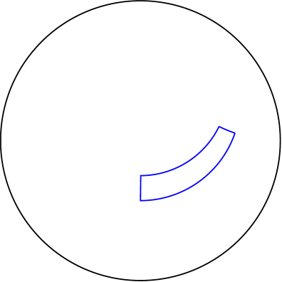
Figure 19: The domain $G$ in the exterior of a horizontal rectangular closed set in the upper half-plane (left) and its image $\hat{G}$ under the auxiliary map $\Psi$ (right) for $d=0.1$.

As in the previous example, the the auxiliary map $w=\Psi(z)$ in (44) is used to transform the domain $G$ onto a domain $\hat{G}$ interior to the unit disk and exterior to a piecewise smooth Jordan curve (see Figure 19). Then $G$ and $\hat{G}$ have the same capacities. We use the function annq with $n=2^{15}$ to compute the capacity of $\hat{G}$ for several values of $d$. When $d=0$, the rectangle reduced to the slit $[0.5\mathrm{i},1+0.5\mathrm{i}]$. By symmetry, the capacity for the half-plane with the horizontal slit $[0.5\mathrm{i},1+0.5\mathrm{i}]$ is $2$ times the capacity for the cases of the domain exterior to the two horizontal slits $[\mathrm{i}/2,1+\mathrm{i}/2]$ and $[-\mathrm{i}/2,1-\mathrm{i}/2]$ considered in Subsection 7.1. Thus, according to the exact capacity presented in Subsection 7.1, the exact capacity for the upper half-plane with the horizontal slit $[0.5\mathrm{i},1+0.5\mathrm{i}]$ is $4.23155794184903$.

For numerical computing of the capacity of the upper half-plane with the slit $[0.5\mathrm{i},1+0.\mathrm{i}]$, we use the method described in Section 6. The obtained result is presented at the bottom of Table 11. The computed approximate value agrees with the exact value with relative error $1.1\times 10^{-9}$.

Finally, the third column in Table 11 shows halves of the computed values of the capacity for the domain presented in this section. The values presented in the third column agrees with the results presented in Table 9 for two rectangle case.

Table 11: The capacity values for the domain exterior to a horizontal rectangle in the upper half-plane.

$d$	$\mathrm{cap}(G)$	$\mathrm{cap}(G)/2$	Time (sec)
0.4	15.1134561077006	7.5567280538503	2.6
0.3	9.10569023215289	4.55284511607644	2.5
0.2	6.77138475734822	3.38569237867411	2.3
0.1	5.37377572427995	2.68688786213998	2.4
0.05	4.81109439601605	2.40554719800803	2.5
0.02	4.48126118775531	2.24063059387766	3.1
0.01	4.36525097360269	2.18262548680134	4.1
0.005	4.30323272661648	2.15161636330824	5.7
0	4.2315579463472	2.1157789731736	23.0

8 The hyperbolic capacity and the elliptic capacity

Let $E$ be a compact and connected set (not a single point) in the unit disk $\mathbb{D}$. In this section, we use the MATLAB function annq in Subsection 2.6 to compute the hyperbolic capacity and the elliptic capacity of the set $E$. Both the hyperbolic capacity and the elliptic capacity are invariants under conformal mappings.

8.1 The hyperbolic capacity

The hyperbolic capacity of $E$, $\mathrm{caph}(E)$, is defined by [42, p. 19]

$$\mathrm{caph}(E)=\lim_{n\to\infty}\left[\max_{z_{1},\ldots,z_{n}\in E}\prod_{1\leq k<j\leq n}\left|\frac{z_{k}-z_{j}}{1-z_{k}\overline{z_{j}}}\right|\right]^{\frac{2}{n(n-1)}}.$$ (45)

For the hyperbolic capacity, we assume $G$ is the bounded doubly connected domain defined by $G=\mathbb{D}\backslash E$ such that $G$ can be mapped conformally onto an annulus $q<|w|<1$. Hence the hyperbolic capacity $\mathrm{caph}(E)$ is given by [13]

$$\mathrm{caph}(E)=q.$$ (46)

The constant $q$ can be computed by the function annq.

8.2 The elliptic capacity

For the compact and connected set $E$, we define the antipodal set $E^{\ast}=\{-1/\overline{a}\,:\,a\in E\}$. Since we assume $E\subset\mathbb{D}$, we have $E\cap E^{\ast}=\emptyset$ (in this case, the set $E$ is called “elliptically schlicht” [13]). The elliptic capacity of $E$, $\mathrm{cape}(E)$, is defined by [13]

$$\mathrm{cape}(E)=\lim_{n\to\infty}\left[\max_{z_{1},\ldots,z_{n}\in E}\prod_{1\leq k<j\leq n}\left|\frac{z_{k}-z_{j}}{1+z_{k}\overline{z_{j}}}\right|\right]^{\frac{2}{n(n-1)}}.$$ (47)

To compute the elliptic capacity, we assume $G$ is the doubly connected domain between $E$ and $E^{\ast}$ such that $G$ can be mapped conformally onto an annulus $r<|w|<1/r$. Then the elliptic capacity is given by [13]

$$\mathrm{cape}(E)=r.$$

Here, the domain $G$ could be bounded or unbounded. We shall use the method described in Section 2 to map the domain $G$ onto an annulus $q<|w|<1$ which is conformally equivalent to the annulus $r<|w|<1/r$ with $r=\sqrt{q}$. Thus, we have

$$\mathrm{cape}(E)=\sqrt{q}.$$ (48)

We compute $q$ using the function annq.

Finally, as our interest in this paper is only in closed and connected subsets $E$ of the unit disk $\mathbb{D}$ and comparing numerically between the values of $\mathrm{cape}(E)$ and $\mathrm{caph}(E)$, it is worth mentioning that Duren and Kühnau [13] have proved that

$$\mathrm{cape}(E)\leq\mathrm{caph}(E),$$

with equality if and only if $E=-E$. This inequality is verified numerically in the following numerical examples.

8.3 A disk

As our first example, we compute the hyperbolic capacity and the elliptic capacity of the disk $E=\{z\in\mathbb{C}\;:\;|z|\leq r\}$, $0<r<1$. For this set $E$, both capacities are equal where [22, 13]

$$\mathrm{caph}(E)=\mathrm{cape}(E)=r.$$

For computing $\mathrm{caph}(E)$, we use the function annq with $\alpha=(1+r)/2$ and $z_{2}=0$ to compute the value of $q$ for the conformal map of the doubly connected domain $G=\mathbb{D}\backslash E$ (see Figure 20 (left)) onto the annulus $q<|w|<1$ and hence $\mathrm{caph}(E)=q$. For $\mathrm{cape}(E)$, the domain $G$ between $E$ and $E^{\ast}$ is the bounded doubly connected domain $r<|z|<1/r$ (see Figure 20 (right)). We use the MATLAB function annq with $\alpha=1$ and $z_{2}=0$ to compute the value of $q$ for the conformal map of this domain $G$ onto the annulus $q<|w|<1$ and hence $\mathrm{cape}(E)=\sqrt{q}$. For both cases, we use $n=2^{12}$ and $0.02\leq r\leq 0.98$. The relative error in the obtained results for $\mathrm{caph}(E)$ and $\mathrm{cape}(E)$ are shown in Figure 21.

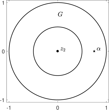
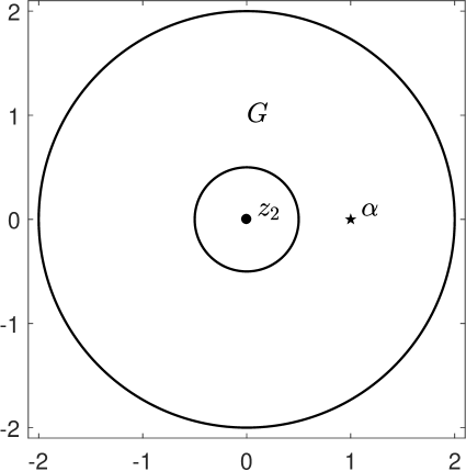
Figure 20: The domain $G$ for computing the hyperbolic capacity (left) and the elliptic capacity (right) of $E=\{z\in\mathbb{C}\;:\;|z|\leq r\}$ for $r=0.5$.

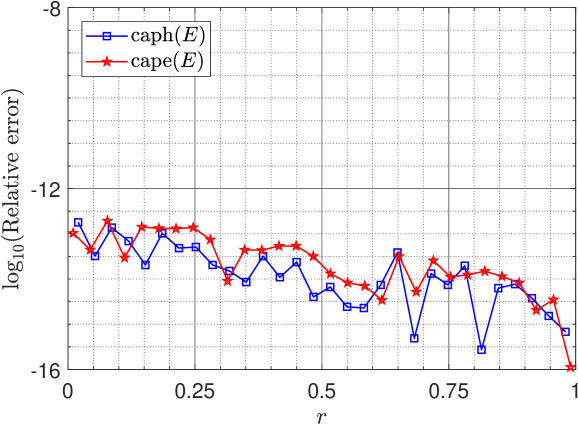
Figure 21: The relative error in the computed capacities $\mathrm{c}(E)$, $\mathrm{caph}(E)$, and $\mathrm{cape}(E)$ for the disk $E=\{z\in\mathbb{C}\;:\;|z|\leq r\}$.

8.4 A square

For the second example, we assume $E$ is the closed set $[-r,r]\times[-r,r]$, $0<r<1/\sqrt{2}$. For computing $\mathrm{caph}(E)$, the domain $G$ is the bounded doubly connected domain exterior to the square and interior to the unit circle (see Figure 22 (left)). We use the function annq with $\alpha=(1+r)/2$ and $z_{2}=0$ to compute $q$ and then $\mathrm{caph}(E)=q$. For $\mathrm{cape}(E)$, the domain $G$ is the bounded doubly connected domain between $E$ and $E^{\ast}$ (see Figure 22 (right)). Hence, $\mathrm{cape}(E)=\sqrt{q}$ where $q$ is computed using the function annq with $\alpha=(r+1/r)/2$ and $z_{2}=0$. For both cases, we use $n=2^{13}$ for $0.02\leq r\leq 0.69$. The obtained results are shown in Figure 23. This set $E$ is symmetric where $E=-E$, and hence $\mathrm{caph}(E)=\mathrm{cape}(E)$.

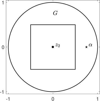
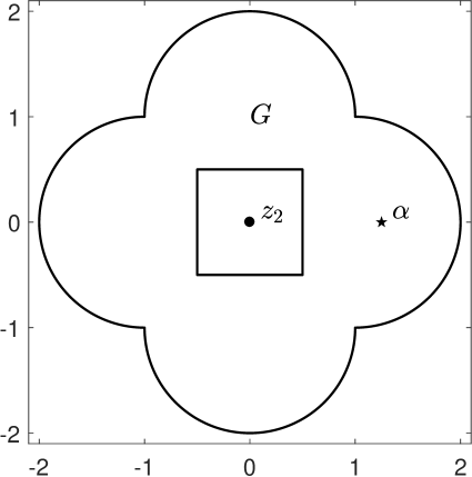
Figure 22: The domain $G$ for computing the hyperbolic capacity (left) and the elliptic capacity (right) of $E=[-r,r]\times[-r,r]$ for $r=0.5$.

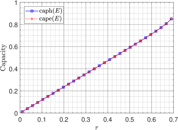
Figure 23: The capacities $\mathrm{caph}(E)$ and $\mathrm{cape}(E)$ for $E=[-r,r]\times[-r,r]$.

8.5 Amoeba-shaped boundary

For the third example, we compute $\mathrm{caph}(E)$ and $\mathrm{cape}(E)$ of $E$ where $E$ is the closed region bordered by the amoeba-shaped boundary $L$ with the parametrization

$$\eta(t)=0.1+0.6\mathrm{i}+0.2\left(e^{\cos t}\cos^{2}2t+e^{\sin t}\sin^{2}2t\right)e^{-\mathrm{i}t},\quad 0\leq t\leq 2\pi.$$

For the hyperbolic capacity $\mathrm{caph}(E)$, the domain $G$ is the bounded doubly connected domain exterior to the curve $L$ and interior to the unit circle (see Figure 24 (left)). Then $\mathrm{caph}(E)=q$ where $q$ is computed using the function annq with $\alpha=0$ and $z_{2}=0.25+0.5\mathrm{i}$. To compute $\mathrm{cape}(E)$, the domain $G$ is the unbounded doubly connected domain exterior to $E$ and $E^{\ast}$ (see Figure 24 (right)). We use the function annq with $z_{1}=0.25+0.5\mathrm{i}$ and $z_{2}=-1/\overline{z_{1}}$ to compute the value of $q$ and hence $\mathrm{cape}(E)=\sqrt{q}$. The approximate values of the capacities $\mathrm{caph}(E)$ and $\mathrm{cape}(E)$ for several values of $n$ are shown in Table 12. As the set $E$ is not symmetric, the presented numerical results confirmed the inequality $\mathrm{cape}(E)<\mathrm{caph}(E)$.

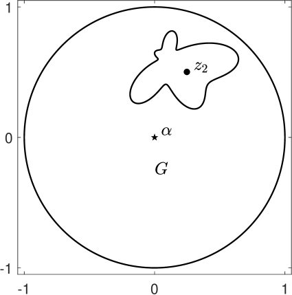
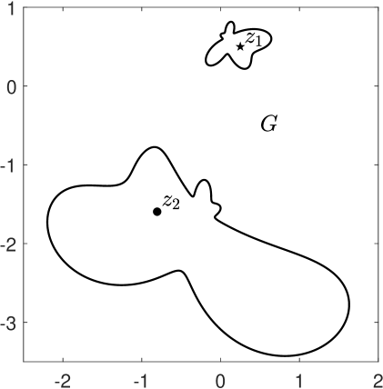
Figure 24: The domain $G$ for computing the hyperbolic capacity (left) and the elliptic capacity (right) of the closed region bordered by the amoeba-shaped boundary $E$.

Table 12: The approximate values of the capacities of the closed region bordered by the amoeba-shaped boundary $E$.

$n$	$\mathrm{caph}(E)$	$\mathrm{cape}(E)$
64	0.521349946390291	0.25872431985379
128	0.521358819409768	0.258724285703159
256	0.521358832558364	0.258724285703154
512	0.521358832558375	0.258724285703153
1024	0.52135883255838	0.258724285703155
2048	0.521358832558369	0.258724285703154
4096	0.521358832558378	0.258724285703156

9 Concluding Remarks

Conformal invariants are important tools for complex analysis with many applications. However, these invariants can be expressed explicitly only in very few special cases. Thus, numerical methods are required to compute these invariants. A numerical method for computing some conformal invariants is presented in this paper. The method can be used for domains with different types of boundaries including domains with smooth or piecewise smooth boundaries. The performance and the accuracy of the presented method is compared to analytic solutions or to previous results whenever analytic solutions or previous results are available. Further, a MATLAB implementation of the proposed method is given in the MATLAB function annq in Subsection 2.6. This MATLAB function was used in almost all examples in this paper to compute the conformal capacity, the hyperbolic capacity and the elliptic capacity. For some examples, an auxiliary procedure is required before using the function annq. The computer codes of the presented computations can be found in the link https://github.com/mmsnasser/cci.

References

- [1] L. Ahlfors, Conformal Invariants, McGraw-Hill, New York, 1973.
- [2] G. D. Anderson, M. K. Vamanamurthy, and M. Vuorinen, Conformal Invariants, Inequalities and Quasiconformal Maps, John Wiley, New York, 1997.
- [3] K. Atkinson, The Numerical Solution of Integral Equations of the Second Kind, Cambridge University Press, Cambridge, 1997.
- [4] A. Austin, P. Kravanja, and L. Trefethen, Numerical algorithms based on analytic function values at roots of unity, SIAM J. Numer. Anal., 52 (2014), pp. 1795–1821.
- [5] D. Betsakos, K. Samuelsson, and M. Vuorinen, The computation of capacity of planar condensers, Publ. Inst. Math. (Beograd) (N.S.), 75 (2004), pp. 233–252.
- [6] S. Bezrodnykh, A. Bogatyrev, S. Goreinov, O. Grigoriev, H. Hakula, and M. Vuorinen, On capacity computation for symmetric polygonal condensers, J. Comput. Appl. Math., 361 (2019), pp. 271–282.
- [7] F. Bowman, Introduction to Elliptic Functions with Applications, English Universities Press Ltd., London, 1953.
- [8] P. Byrd and M. D. Friedman, Handbook of elliptic integrals for engineers and scientists. Second edition, revised., Springer-Verlag, Berlin, 1971.
- [9] D.Dautova, S.Nasyrov, and M.Vuorinen, Conformal module of the exterior of two rectilinear slits, Comput. Methods Funct. Theory, (2020), p. arXiv:1908.02459.
- [10] T. DeLillo, A. Elcrat, and E. Kropf, Calculation of resistances for multiply connected domains using Schwarz-Christoffel transformations, Comput. Methods Funct. Theory, 11 (2011), pp. 725–745.
- [11] T. Driscoll and L. Trefethen, Schwarz-Christoffel mapping, Cambridge University Press, Cambridge, 2002.
- [12] V. Dubinin, Condenser Capacities and Symmetrization in Geometric Function Theory, Springer, Basel, 2014.
- [13] P. Duren and R. Kühnau, Elliptic capacity and its distortion under conformal mapping, J. Anal. Math., 89 (2003), pp. 317–335.
- [14] M. Embree and L. Trefethen, Green’s functions for multiply connected domains via conformal mapping, SIAM Rev., 41 (1999), pp. 745–761.
- [15] J. Garnett and D. Marshall, Harmonic measure, Cambridge University Press, Cambridge, 2008.
- [16] L. Greengard and Z. Gimbutas, FMMLIB2D: A MATLAB toolbox for fast multipole method in two dimensions, version 1.2. ed., 2012. http://www.cims.nyu.edu/cmcl/fmm2dlib/fmm2dlib.html. Accessed 1 Jan 2018.
- [17] H. Hakula, A. Rasila, and M. Vuorinen, On moduli of rings and quadrilaterals: algorithms and experiments, SIAM J. Sci. Comput., 33 (2011), pp. 279–302.
- [18] , Computation of exterior moduli of quadrilaterals, Electron. Trans. Numer. Anal., 40 (2013), pp. 436–451.
- [19] , Conformal modulus on domains with strong singularities and cusps, Electron. Trans. Numer. Anal., 48 (2018), pp. 462–478.
- [20] P. Hariri, R. Klén, and M. Vuorinen, Conformally Invariant Metrics and Quasiconformal Mappings, Springer Monographs in Mathematics, Springer, Switzerland, 2020.
- [21] L. Keen and N. Lakic, Hyperbolic geometry from a local viewpoint, Cambridge University Press, Cambridge, 2007.
- [22] S. Kirsch, Transfinite diameter, Chebyshev constant and capacity, in Handbook of Complex Analysis: Geometric Function Theory, Vol. 2, R. Kühnau, ed., Elsevier, Amsterdam, 2005, pp. 243–308.
- [23] R. Kress, A Nyström method for boundary integral equations in domains with corners, Numer. Math., 58 (1990), pp. 145–161.
- [24] , Linear Integral Equations, Springer, New York, 2014.
- [25] R. Kühnau, ed., Handbook of complex analysis: geometric function theory. Vol. 1, 2002, Vol. 2, 2005, Elsevier Science B.V., Amsterdam.
- [26] P. Kythe, Handbook of conformal mappings and applications, Taylor & Francis Group, Boca Raton, 2019.
- [27] J. Liesen, O. Séte, and M. Nasser, Fast and accurate computation of the logarithmic capacity of compact sets, Comput. Methods Funct. Theory, 17 (2017), pp. 689–713.
- [28] M. Nasser, Numerical conformal mapping via a boundary integral equation with the generalized Neumann kernel, SIAM J. Sci. Comput., 31 (2009), pp. 1695–1715.
- [29] , Numerical conformal mapping of multiply connected regions onto the second, third and fourth categories of Koebe canonical slit domains, J. Math. Anal. Appl., 382 (2011), pp. 47–56.
- [30] , Fast solution of boundary integral equations with the generalized Neumann kernel, Electron. Trans. Numer. Anal., 44 (2015), pp. 189–229.
- [31] , Numerical computing of preimage domains for bounded multiply connected slit domains, J. Sci. Comput., 78 (2019), pp. 582–606.
- [32] M. Nasser and F. Al-Shihri, A fast boundary integral equation method for conformal mapping of multiply connected regions, SIAM J. Sci. Comput., 33 (2013), pp. A1736–A1760.
- [33] M. Nasser and C. Green, A fast numerical method for ideal fluid flow in domains with multiple stirrers, Nonlinearity, 31 (2018), pp. 815–837.
- [34] M. Nasser, A. Murid, and Z. Zamzamir, A boundary integral method for the Riemann-Hilbert problem in domains with corners, Complex Var. Elliptic Equ., 53 (2008), pp. 989–1008.
- [35] M. Nasser and M. Vuorinen, Conformal invariants in simply connected domains, (2020), p. arXiv:2001.10182.
- [36] , Numerical computation of the capacity of generalized condensers, J. Comput. Appl. Math., 377 (2020), p. 112865.
- [37] F. Olver, D. Lozier, R. Boisvert, and C. W. Clark, eds., NIST Handbook of Mathematical Functions, Cambridge University Press, Cambridge, 2010.
- [38] N. Papamichael and N. Stylianopoulos, Numerical conformal mapping: Domain decomposition and the mapping of quadrilaterals, World Scientific, New Jersey, 2010.
- [39] E. Saff and V. Totik, Logarithmic potentials with external fields, Springer-Verlag, Berlin, 1997.
- [40] R. Schinzinger and P. Laura, Conformal mapping. Methods and applications, Dover Publications, Inc., New York, 2003.
- [41] L. Trefethen and J. Weideman, The exponentially convergent trapezoidal rule, SIAM Review, 56 (2014), pp. 385–458.
- [42] A. Vasil’ev, Moduli of Families of Curves for Conformal and Quasiconformal Mappings, Springer-Verlag, Berlin, 2002.
- [43] M. Vuorinen, Conformal invariants and quasiregular mappings, J. Anal. Math., 45 (1985), pp. 69–115.
- [44] , Conformal geometry and quasiregular mappings. Lecture Notes in Mathematics, Springer-Verlag, Berlin, 1988.
- [45] R. Wegmann and M. Nasser, The Riemann-Hilbert problem and the generalized Neumann kernel on multiply connected regions, J. Comput. Appl. Math., 214 (2008), pp. 36–57.