Propagator from Nonperturbative Worldline Dynamics

Abstract.

We use the worldline representation for correlation functions together with numerical path integral methods to extract nonperturbative information about the propagator to all orders in the coupling in the quenched limit (small-$N_{\text{f}}$ expansion). Specifically, we consider a simple two-scalar field theory with cubic interaction (S²QED) in four dimensions as a toy model for QED-like theories. Using a worldline regularization technique, we are able to analyze the divergence structure of all-order diagrams and to perform the renormalization of the model nonperturbatively. Our method gives us access to a wide range of couplings and coordinate distances. We compute the pole mass of the S²QED electron and observe sizable nonperturbative effects in the strong-coupling regime arising from the full photon dressing. We also find indications for the existence of a critical coupling where the photon dressing compensates the bare mass such that the electron mass vanishes. The short distance behavior remains unaffected by the photon dressing in accordance with the power-counting structure of the model.

1. Introduction

In addition to the universal tool of Feynman diagram calculus for perturbative expansions, quantum field theory has given rise to a wide range of methods to deal with systems with many degrees of freedom. The present work is based on the worldline method [1, 2, 3, 4, 5, 6, 7, 8, 9] which can be useful in both perturbative as well as nonperturbative contexts [10, 11, 12, 13, 14, 15, 16, 17, 18, 19, 20, 21, 22, 23, 24, 25, 26, 27].

In addition to the systematic expansion in powers of a small parameter, e.g., a coupling, the topology of diagrams is an ordering principle of Feynman diagram calculus that is also extensively used in modern computer-algebraic realizations, e.g. [28]. As a consequence, single diagrams or single topologies may not respect the symmetries of a theory individually, but a sum over topologies may be needed in order to preserve a symmetry to a given order in the parametric expansion. By contrast, the worldline formulation allows to assess symmetry constraints already on the basis of individual contributions. This is, because subclasses of different topologies can be combined into a single worldline expression, cf. [9, 29].

Even beyond perturbative expansion, it has already been known in the early works on the worldline formalism [3] that whole subclasses of infinitely many Feynman diagrams can be combined into a single closed form expression in specific theories. A prominent example is given by scalar quantum electrodynamics (QED), where all diagrams contributing to the one-particle irreducible (1PI) effective action with one charged-particle loop but arbitrarily many internal photon exchanges can be written as one worldline integral [10]. Introducing $N_{\text{f}}$ flavors of charged particles, this subclass of Feynman diagrams provides the leading-order result of a small-$N_{\text{f}}$ expansion but remains fully nonperturbative in the gauge coupling.

Obtaining nonperturbative results from such all-order expressions is nevertheless challenging, since their evaluation also requires a nonperturbative way to perform the necessary renormalization, i.e., the fixing of physical parameters. In fact, a whole research program has been initiated to cross-check the result for the Schwinger pair production rate evaluated from the all-order worldline expression by semiclassical instanton methods [10] with explicit higher-loop calculations [30, 31, 32, 33, 29], the latter requiring an explicit treatment of the mass renormalization. If semiclassical methods turned out to be reliable also at higher loop order, many studies on Schwinger pair production using worldline instanton methods [20, 34, 35, 36, 37, 38, 39, 40] could be generalized beyond perturbative loop expansions. Also nonperturbative variational approximation techniques have been developed and successfully applied to studies of bound-state properties and self-energies [41, 42, 43, 44, 11, 16, 21]. Recently, the worldline representation of field theory and its relation to string theory has been used to propose a new way of defining UV complete field theories [45].

In order to make progress with nonperturbative worldline techniques, we use two ingredients as proposed in [18]: first, we use a double scalar model to which we refer as S²QED. From the worldline perspective, it is structurally similar to QED, but ignores the spin of both electrons and photons. It is super-renormalizable in $D=4$ spacetime dimensions, such that one-loop renormalization suffices to fix the physical parameters. Second, we use numerical Monte Carlo worldline techniques [46, 47, 48, 49, 50, 51, 52] to nonperturbatively evaluate the worldline path integral. Whereas previous work in this direction has concentrated on quantum effective actions or energies [10, 18, 49, 34] or bound-state amplitudes [16, 15, 21], we investigate the propagator of the “charged” scalar nonperturbatively in this work. The worldline expression for this propagator includes all Feynman diagrams of arbitrary (scalar) photonic self-energy corrections and thus allows to extract information about the decay of nonperturbative correlations with distance and the dependence on the coupling strength in this model.

While the divergence structure of the scalar model is considerably simpler as in renormalizable models, the practical problem of isolating and subtracting the divergent subdiagrams still persists also in this super-renormalizable model. We show that this can be performed with the aid of determining probability distribution functions (PDF) for suitable building blocks of worldline observables. For this, we generalize a technique introduced in [18] to the computation of the propagator. Similar methods have also been applied to numerical worldline computations of Schwinger pair production [53] and recently to high-accuracy results of quantum mechanical potential problems [54, 55]. In the present case, the use of a suitable analytic fit function for the PDF also allows to extrapolate the nonperturbative results to parameter regimes where a direct simulation is computationally expensive.

Specifically, we obtain a semi-analytical expression for the electron propagator, i.e. an analytical expression in which all the numerical information gathered from the worldline numerics is implemented through a set of parameters. This expression greatly simplifies the subsequent analysis, mainly focusing on the physical (pole) mass. We observe that the physical mass gets dressed in a way that suggests the existence of a critical coupling for which the pole mass vanishes. Moreover, there is a clear enhancement of this behaviour arising from the all-order photon corrections in our nonperturbative expression compared with the one-loop result.

In the small distance regime, our nonperturbative results for the correlation function are compatible with a vanishing anomalous dimension. This indicates that the superrenormalizable structure of the model suggested by power-counting also persists beyond perturbation theory.

The paper is organized as follows: in Sect. 2 we begin introducing S²QED and deriving the analytical expression used througout the article for the propagator of the “charged” scalar. The propertime discretization of this propagator is presented in Sect. 3 as a method to regularize the expressions and a closed formula for the one-loop contribution to the propagator is obtained. In possession of this analytic background, we show in Sect. 4 our numerical results. Firstly, a comparison with a one-loop expansion is done in Sect. 4.1. Secondly, we analyse the probability distribution function for the potential involved in our model in Sect. 4.2. Thirdly, in Sect. 4.3 we study and discuss the Worldline Montecarlo results obtained for the propagator of the charged scalar. We state our conclusions in Sect. 5, while we leave an extensive analysis of the new $v$ lines algorithm to App. A. Finally, the remaining appendices deal in detail with the one-loop expressions (App. B), the asymptotics of the discretized potential (App. C), the self-energy in different regularizations (App. D) and the large-distance asymptotics of the one-loop propagator (App. E).

2. Worldline formalism for S²QED

Following [18], we consider S²QED, a quantum field theory with two interacting real scalar fields in $D$-dimensional Euclidean spacetime with cubic interaction, as described by the Lagrangian

$$\mathcal{L}=\frac{1}{2}(\partial_{\mu}\phi)^{2}+\frac{1}{2}m^{2}\phi^{2}+\frac{1}{2}(\partial_{\mu}A)^{2}-\frac{i}{2}hA\phi^{2}.$$ (1)

The model is designed to resemble QED with $A$ corresponding to the massless photon, and $\phi$ representing the charged particle (electron). Apart from a global $\mathbbm{Z}_{2}$ symmetry for the $\phi$ field, there is actually no local symmetry that would play a similar role as in QED; hence the model if taken literally can be expected to behave rather differently compared with QED. Nevertheless, the important point for the present purpose is that the model gives rise to a Feynman diagrammar with the same topological features as QED – and also has a worldline representation very similar to that of QED. This model is used in different versions, mostly with a real coupling, for many purposes, e.g., lately also for studying the decoupling in curved spaces [56] or unitarity and ghosts after the inclusion of higher-derivative terms [57].

In the present work, we are interested in the propagator, i.e. the two-point correlator, of the $\phi$ field which can be derived from first principles from the generating functional

$$Z[\eta] = e^{W[\eta]}=\int\mathcal{D}A\mathcal{D}\phi e^{-\int\mathcal{L}+\int\eta\phi}$$ (2)

$$= \int\mathcal{D}A\,\det{}^{-1/2}\big{(}K[A]\big{)}\,e^{-\frac{1}{2}\int(\partial_{\mu}A)^{2}+\frac{1}{2}\int\eta K^{-1}[A]\eta},$$

where $\eta(x)$ is an auxiliary source for the $\phi$ field, and $K[A]=-\partial^{2}+m^{2}-ihA$ denotes the Klein-Gordon operator in the background of an $A$ field. In the second line of eq. (2), we have performed the Gaußian $\phi$ integration. The $\phi$ propagator, being the connected part of the two-point function, can straightforwardly be obtained from the Schwinger functional $W[\eta]$,

$$G(x_{\text{F}},x_{\text{I}}) = \frac{\delta^{2}W[\eta]}{\delta\eta(x_{\text{F}})\delta\eta(x_{\text{I}})}\bigg{|}_{\eta=0}$$ (3)

$$= \frac{1}{Z[0]}\int\mathcal{D}A\,\det{}^{-1/2}\big{(}K[A]\big{)}\,e^{-\frac{1}{2}\int(\partial_{\mu}A)^{2}}\,K^{-1}[A](x_{\text{F}},x_{\text{I}}).$$

So far, our derivation has been exact. From now on, we confine ourselves to the leading order in a small-$N_{\text{f}}$ expansion. Formally introducing $N_{\text{f}}$ flavors of the $\phi$ field, the scalar determinant is of order $\det{}^{-1/2}\big{(}K[A]\big{)}=e^{-\frac{1}{2}\ln\det\big{(}K[A]\big{)}}=e^{-\frac{1}{2}\text{Tr}\ln\big{(}K[A]\big{)}}\sim e^{-\mathcal{O}(N_{\text{f}})}$. Thus, the determinant can be dropped to leading order which is reminiscent to a quenched approximation.

The worldline representation can now be introduced by rewriting the inverse Klein-Gordon operator as a propertime integral, and successively interpreting this operator as the Hamiltonian of a quantum-mechanical propertime evolution. The latter is then written in terms of a Feynman path integral,

$$K^{-1}[A](x_{\text{F}},x_{\text{I}}) = \int_{0}^{\infty}dT\,\langle x_{\text{F}}|e^{-K[A]T}|x_{\text{I}}\rangle,$$ (4)

$$= \frac{1}{(4\pi)^{D/2}}\int_{0}^{\infty}\frac{dT}{T^{D/2}}\,e^{-m^{2}T}e^{-\frac{(x_{\text{F}}-x_{\text{I}})^{2}}{4T}}\Big{\langle}e^{ih\int_{0}^{T}d\tau A(x(\tau))}\Big{\rangle}_{x_{\text{I}}}^{x_{\text{F}}}\!,$$

where we have introduced the worldline expectation value with respect to the free path integral from $x_{\text{I}}$ to $x_{\text{F}}$ in propertime $T$ for an observable $O[x]$,

$$\Big{\langle}O[x]\Big{\rangle}_{x_{\text{I}}}^{x_{\text{F}}}:=\frac{\int_{x(0)=x_{\text{I}}}^{x(T)=x_{\text{F}}}\mathcal{D}x\,O[x]\,e^{-\frac{1}{4}\int_{0}^{T}d\tau\dot{x}^{2}}}{\int_{x(0)=x_{\text{I}}}^{x(T)=x_{\text{F}}}\mathcal{D}x\,e^{-\frac{1}{4}\int_{0}^{T}d\tau\dot{x}^{2}}}.$$ (5)

Inserting eq. (4) into eq. (3), we can interchange the worldline expectation value with the functional integral over $A$ fields. Introducing the current of a $\phi$ particle on the worldline,

$$j(z)=ih\int_{0}^{T}d\tau\,\delta^{(D)}(z-x(\tau))\quad\Rightarrow\quad e^{ih\int_{0}^{T}d\tau A(x(\tau))}=e^{\int jA},$$ (6)

the functional integral over the $A$-field configurations is Gaußian, resulting in

$$\frac{1}{Z[0]}\int\mathcal{D}A\,e^{-\frac{1}{2}\int(\partial_{\mu}A)^{2}+\int jA}=e^{\frac{1}{2}\int j\Delta j}.$$ (7)

Note that also the normalization $Z[0]$ has to be computed within the small-$N_{\text{f}}$ approximation. In eq. (7), $\Delta=(-\partial^{2})^{-1}$ denotes the propagator of the photonic $A$ field which in coordinate space reads

$$\Delta(x_{1},x_{2})=\frac{\Gamma\left(\frac{D-2}{2}\right)}{4\pi^{D/2}}\frac{1}{|x_{1}-x_{2}|^{D-2}}.$$ (8)

We observe that the photon fluctuations can be summarized in a current-current interaction of the $\phi$ field being represented by a worldline trajectory with itself. Using the explicit representation of the current (6), we get

$$\frac{1}{2}\int j\Delta j = -\frac{h^{2}}{8\pi^{D/2}}\Gamma\left({\scriptstyle\frac{D-2}{2}}\right)\int_{0}^{T}d\tau_{1}d\tau_{2}\frac{1}{|x_{1}-x_{2}|^{D-2}}$$ (9)

$$=: -gV[x],\quad g:=\frac{h^{2}}{8\pi^{D/2}}\Gamma\left({\scriptstyle\frac{D-2}{2}}\right).$$

Here and in the following, we use the convention $x_{i}=x(\tau_{i})$. The coupling $g$ plays the role of a fine-structure constant in this model, and $V[x]$ can be viewed as a potential for the interactions of a worldline with itself. Inserting these findings into eq. (3), we end up with the worldline representation of the (unrenormalized) field propagator to leading order in the small-$N_{\text{f}}$ limit,

$$G(x_{\text{F}},x_{\text{I}})=\frac{1}{(4\pi)^{D/2}}\int_{0}^{\infty}\frac{dT}{T^{D/2}}\,e^{-m^{2}T}\,e^{-\frac{(x_{\text{F}}-x_{\text{I}})^{2}}{4T}}\Big{\langle}e^{-gV[x]}\Big{\rangle}_{x_{\text{I}}}^{x_{\text{F}}},$$ (10)

in agreement with the formula given in [18]. It is obvious that this representation is nonperturbative in the coupling $g$ as it contains powers of $g$ to all orders. In a Feynman-diagram language, eq. (10) summarizes all possible diagrams with one $\phi$-particle line and an arbitrary number of photonic $A$-field radiative corrections in one single expression. There is no restriction on the diagram topology (e.g. 1PI or “rainbow” diagrams): the expression also includes one-particle reducible as well as crossing-rainbow diagrams. The challenge pursued in the following sections is to evaluate the worldline path integral.

3. Weak-coupling expansion and renormalization

Let us start with the noninteracting limit $g\to 0$. In that case, there is no photonic contribution, and the propagator of eq. (10) reduces to the free Green’s function of the massive Klein-Gordon operator. Upon performing the $T$ integral, we arrive at an expression in terms of a Macdonald function,

$$G_{0}(\Delta x)=\frac{1}{(2\pi)^{D/2}}\left(\frac{m^{2}}{\Delta x^{2}}\right)^{(D-2)/4}K_{(D-2)/2}(m\Delta x),\quad\Delta x=|x_{\text{F}}-x_{\text{I}}|.$$ (11)

Because of translational invariance, the propagator depends only on the distance of the endpoints also in the presence of photonic interactions.

At weak-coupling, eq. (10) suggests a perturbative expansion in powers of the coupling, resulting in higher-order worldline correlators of the interaction potential, $(-g)^{n}\big{\langle}V^{n}[x]\big{\rangle}_{x_{\text{I}}}^{x_{\text{F}}}$. Because of the superrenormalizable structure of the theory, we expect the divergence relevant for mass renormalization to appear only to leading order in the coupling $g$. Once this one-loop order is renormalized, all remaining terms should be finite. Thus, a careful analysis of the leading order expectation value $\big{\langle}V[x]\big{\rangle}_{x_{\text{I}}}^{x_{\text{F}}}$ is a crucial building block for the nonperturbative study. This expression can be studied straightforwardly with continuum worldline techniques [9], allowing to make contact with standard regularization schemes such as propertime or dimensional regularization.

In order to make direct contact with the full numerical studies below, we proceed differently and study this expectation value by regulating the path integral in terms of a propertime lattice. For this, we first perform a rescaling of the worldlines, such that their distribution becomes independent of the propertime [46]

$$y(t):=\frac{1}{\sqrt{T}}x(Tt),\quad t\in[0,1]\quad\Rightarrow\quad\int_{0}^{T}d\tau\,\dot{x}^{2}(\tau)=\int_{0}^{1}dt\,\dot{y}^{2}(t).$$ (12)

We call the worldlines parametrized by $y(t)$ unit lines. Accordingly, the initial and final points of the unit lines are related to the physical initial and final point by rescaling, $y_{\text{I}}=y(0)=x_{\text{I}}/\sqrt{T}$, $y_{\text{F}}=y(1)=x_{\text{F}}/\sqrt{T}$. Moreover, the worldline interaction potential can be rescaled,

$$V[x]=\int_{0}^{T}\frac{d\tau_{1}d\tau_{2}}{|x_{1}-x_{2}|^{D-2}}=T^{3-D/2}\int_{0}^{1}\frac{dt_{1}dt_{2}}{|y_{1}-y_{2}|^{D-2}},\quad\big{\langle}V[x]\big{\rangle}_{x_{\text{I}}}^{x_{\text{F}}}\equiv\big{\langle}V[y]\big{\rangle}_{y_{\text{I}}}^{y_{\text{F}}}.$$ (13)

Subsequently, we discretize the unit lines, by slicing the rescaled propertime $t$ into $N$ time intervals,

$$y(t)\quad\to\quad y(t_{i})=y_{i}\in\mathbbm{R}^{D},\quad t_{i}=\frac{i}{N},\quad i,=0,1,\dots,N.$$ (14)

Note that the spacetime remains continuous in this approach. We discretize the worldline kinetic term in eq. (12) by a standard nearest-neighbor difference quotient (see App. A). The integrals in the worldline interaction potential, in the discretized form, then correspond to Riemann sums over the $N$ propertime slices

$$V[y]=\frac{2T^{3-D/2}}{N^{2}}\sum_{l=0}^{N-2}\sum_{n=l+1}^{N-1}\frac{1}{|y_{l}-y_{n}|^{D-2}}.$$ (15)

Here, we have removed the coincident points for $l=n$, where the self-interaction potential in the discretized version is ill-defined. The associated short-distance singularity will nevertheless be approached in the propertime continuum limit for increasing $N$, as the discretized version of the probability distribution (12) corresponds to a random walk for which $|y_{i}-y_{i-1}|\sim 1/\sqrt{N}$. Hence we expect a divergence to appear in the limit $N\to\infty$. We have checked that a regularization of the coincident point limit by shifting the denominator $|y_{l}-y_{n}|^{D-2}\to|y_{l}-y_{n}|^{D-2}+\delta$ but including the $n=l$ terms in the sum yields the same divergences in the limit $\delta\to 0$.

The procedure of keeping $N$ finite hence regularizes the worldline expressions. As shown in the following, it allows for meaningful numerical computations of relevant quantities as well as for a controlled study of the $N\to\infty$ limit. It is however important to note that there is a decisive difference to a conventional momentum-space or short-distance cutoff: as $\delta y\sim 1/\sqrt{N}$, we have $\Delta x\sim\sqrt{T}/\sqrt{N}$. For a given fixed $N$, fluctuations associated with different propertimes $T$ are thus regularized at different length scales. As a consequence, our final results will differ from those obtained by a standard regularization scheme not only by a simple scheme change, i.e., a shift of finite constants. Instead, our worldline regularization will be linked to a standard regularization by a finite spacetime- or momentum-dependent transformation. The connection is worked out in App. D on the one-loop level. For reasons of clarity, we use the worldline regularization in the main text for our nonperturbative analysis.

Coming back to the expectation value of the worldline interaction potential, it has to be computed for an ensemble of open worldlines interconnecting $y_{\text{I}}$ and $y_{\text{F}}$ with a Gaußian velocity distribution. For our numerical studies below, we use a new algorithm (which we call $v$ lines) to generate such discretized random paths. This construction is detailed in App. A and is tested considering a simple model in App. A.1.

For the one-loop contribution to the propagator in the discretized formulation, we now need to compute

$$\left\langle V[y]\right\rangle^{y_{\text{F}}}_{y_{\text{I}}}=\mathcal{N}\int_{y_{\text{I}}}^{y_{\text{F}}}\mathcal{D}y\,e^{-\frac{N}{4}\sum_{i=1}^{i=N}(y_{i}-y_{i-1})^{2}}V[y],$$ (16)

with the discretized representation (15) of the interaction potential, and the abbreviations,

$$\mathcal{N}^{-1}:={\int^{y_{\text{F}}}_{y_{\text{I}}}\mathcal{D}y\,e^{-\frac{N}{4}\sum_{i=1}^{i=N}(y_{i}-y_{i-1})^{2}}},\quad\mathcal{D}y:=\prod_{j=1}^{N-1}d^{D}y_{j}.$$ (17)

The worldline integrations can be performed analytically by using the Fourier representation of the interaction kernel, cf. eq. (8),

$$\left\langle V[y]\right\rangle^{y_{\text{F}}}_{y_{\text{I}}}=\frac{8T^{3-D/2}}{N^{2}\Gamma\left(\frac{D-2}{2}\right)}\sum_{0=l<n}^{N-1}\mathcal{N}\int_{y_{\text{I}}}^{y_{\text{F}}}\mathcal{D}y\,e^{-\frac{N}{4}\sum_{i}(y_{i}-y_{i-1})^{2}}\int\frac{d^{D}p}{(4\pi)^{D/2}}\frac{e^{ip(y_{l}-y_{n})}}{p^{2}}.$$ (18)

We observe that all $y_{i}$ integrals still remain Gaußian and hence can be performed by a suitable completion of the square. The corresponding computation can be performed along the same lines as for the construction of the $v$ lines algorithm, except for a different completion of the squares at positions $l$ and $n$. With the details highlighted in App. B, we arrive at

$$\left\langle V[y]\right\rangle^{y_{\text{F}}}_{y_{\text{I}}} = 2\frac{T^{3-D/2}}{(\Delta y)^{D-2}}\sum_{n=1}^{N-1}\frac{N^{D-4}(N-n)}{n^{D-2}}\left[1-\frac{\Gamma\left(\frac{D-2}{2},\frac{n\Delta y^{2}}{4(N-n)}\right)}{\Gamma\left(\frac{D-2}{2}\right)}\right],$$ (19)

where $\Delta y=|y_{\text{F}}-y_{\text{I}}|$, and $\Gamma(a,z)$ denotes the incomplete gamma function. Let us from now on specialize to the case of $4$-dimensional spacetime, $D=4$, yielding

$$\left\langle V[y]\right\rangle^{y_{\text{F}}}_{y_{\text{I}}} = 2\frac{T}{\Delta y^{2}}\sum_{n=1}^{N-1}\frac{(N-n)}{n^{2}}\left[1-e^{-\frac{n\Delta y^{2}}{4(N-n)}}\right]$$ (20)

$$= 2\frac{T^{2}}{\Delta x^{2}}\sum_{n=1}^{N-1}\frac{(N-n)}{n^{2}}\left[1-e^{-\frac{n\Delta x^{2}}{4T(N-n)}}\right],$$ (21)

where we reinstated the dimensionful physical distance in the last line. It is instructive to study the short-distance limit,

$$\left\langle V[y]\right\rangle_{y_{\text{I}}}^{y_{\text{F}}} = \frac{1}{2}T\sum_{n=1}^{N-1}\frac{1}{n}+\mathcal{O}(\Delta y^{2})$$

$$= \frac{1}{2}T\,H_{N-1}+\mathcal{O}(\Delta y^{2})$$

$$= \frac{1}{2}T\,\big{(}\ln N+\gamma\big{)}+\mathcal{O}(\Delta y^{2},1/N).$$

We observe that the short-distance limit is essentially given by the harmonic number $H_{N-1}$ which diverges logarithmically for large $N$ with the constant part given by the Euler-Mascheroni constant $\gamma$. The analytical result (3) for the large-N expectation value of the worldine interaction potential for closed worldlines, i.e., $\Delta y=0$, is in fact in good agreement with the numerical estimates of [18].

The logarithmic divergence discovered in eq. (3) is a UV divergence and indicates the necessity of performing a renormalization of physical parameters. In the present model, simple power-counting tells us that such a divergence is expected to correspond to a counterterm $\delta m^{2}$, denoting the additive renormalization of the mass (a possible wave function renormalization $Z_{\phi}$ remains finite). In order to illustrate how the divergence relates to mass renormalization, we go back to eq. (10) and concentrate on two factors of the propertime integrand in the short distance limit:

$$e^{-m^{2}T}\Big{\langle}e^{-gV[x]}\Big{\rangle}_{x_{\text{I}}}^{x_{\text{F}}} = e^{-m^{2}T}\sum_{k=0}^{\infty}\frac{(-g)^{k}}{k!}\big{\langle}V[x]^{k}\big{\rangle}_{x_{\text{I}}}^{x_{\text{F}}}$$ (23)

$$= e^{-m^{2}T}\sum_{k=0}^{\infty}\frac{(-g)^{k}}{k!}\left(\big{\langle}V[x]\big{\rangle}_{x_{\text{I}}}^{x_{\text{F}}}\right)^{k}+\text{connected}$$

$$= e^{-m^{2}T}e^{-g\langle V[x]\rangle_{x_{\text{I}}}^{x_{\text{F}}}}+\text{connected}.$$

Here “connected” denotes the connected parts of operator products of the self-interaction potential; e.g., to second order in $V$, the connected part would essentially be given by $\langle V[x]V[x]\big{\rangle}_{x_{\text{I}}}^{x_{\text{F}}}-\left(\langle V[x]\big{\rangle}_{x_{\text{I}}}^{x_{\text{F}}}\right)^{2}$. These connected parts contribute to 1PI diagrams with overlapping photon radiative corrections, which are power-counting finite. Therefore, the mass shift is fully contained in the disconnected part written explicitly in eq. (23). This suggests to define the following finite mass parameter

$$m_{\text{WR}}^{2}:=m^{2}-\delta m^{2},\quad\delta m^{2}=-\frac{g}{2}\big{(}\ln N+\gamma\big{)},$$ (24)

where we understand the bare mass $m$ to be implicitly $N$ dependent, such that $m_{\text{WR}}$ is kept at a finite fixed value in the limit $N\to\infty$. In the following, $m_{\text{WR}}$ will serve as a fixed input parameter representing a finite mass parameter of the theory in the worldline regularization. Moreover, we use $m_{\text{WR}}$ in the remainder of this work to set the scale for all other dimensionful quantities.

To sum up, we conclude that the mass-renormalized version of the propagator (10) in worldline representation and for $D=4$ reads,

$$G(x_{\text{F}},x_{\text{I}})=\frac{1}{(4\pi)^{2}}\int_{0}^{\infty}\frac{dT}{T^{2}}\,e^{-m_{\text{WR}}^{2}T}\,e^{-\frac{(x_{\text{F}}-x_{\text{I}})^{2}}{4T}}\Big{\langle}e^{-\delta m^{2}T-gV[x]}\Big{\rangle}_{x_{\text{I}}}^{x_{\text{F}}},$$ (25)

yielding a finite result also in the limit $N\to\infty$, because of eq. (3).

4. Worldline Monte Carlo for the propagator

Let us now turn to an evaluation of the worldline path integrals by a Monte Carlo procedure. For this, we generate an ensemble of open worldlines extending over the dimensionless distance $\Delta y=y_{\text{F}}-y_{\text{I}}$ using the $v$ lines algorithm. This ensemble is characterized by the total number $n_{\text{L}}$ of lines and the number $N$ of discretization points per line. The worldline expectation value of an operator $\mathcal{O}[y]$ is then estimated as

$$\left\langle\mathcal{O}[y]\right\rangle^{y_{\text{F}}}_{y_{\text{I}}}\simeq\frac{1}{n_{\text{L}}}\sum_{\ell=1}^{n_{\text{L}}}\mathcal{O}[y_{\ell}].$$ (26)

The full continuum result would be obtained in the limit $n_{\text{L}}\to\infty$ and $N\to\infty$.

4.1. One-loop comparison

As a benchmark test, we compare the results of a Monte Carlo simulation for the expectation value of the interaction potential with the analytical results, cf. eq. (20); this corresponds to a check at the one-loop level. For this purpose, we generate ensembles of $n_{\text{L}}=100000$ lines for an increasing number $N$ of points per line extending over a distance $\Delta y=\left|y_{F}-y_{I}\right|$. In the following, we set the propertime $T=1$ without loss of generality; for dimensional reasons, it is clear that $V[y]$ scales linearly with $T$, cf. eq. (13).

In Fig. 1, we show the behavior of the expectation value of the potential $\langle V\rangle_{y_{\text{I}}}^{y_{\text{F}}}$ as a function of the number of points per line $N$ (in a $\log_{2}$ scale); the left (right) panel corresponds to $\Delta y=1$ ($\Delta y=14$). The error bars for the numerical data correspond to the root-mean-square (RMS) of the expectation value in the given ensemble. The worldline Monte Carlo (WMC) data is compared to the analytical expression of eq. (20) (red solid line).

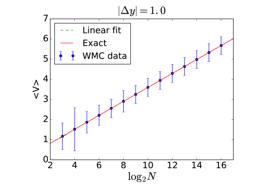
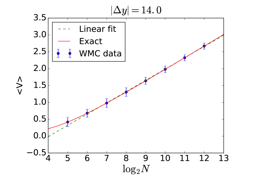
Figure 1. Mean value $\langle V\rangle$ of the potential as a function of $\log_{2}N$, the base two logarithm of the number $N$ of point per loops, for lines whose endpoints distance are $\Delta y=1$ (left) and $\Delta y=14$ (right). The exact analytic expression (solid red line) and the fitting with a straight line (dashed green line) are also shown.

The agreement between the numerical data and the analytical result is very satisfactory for all $N$ and $\Delta y$. The RMS error appears to overestimate the true error. For larger $\Delta y$, the error becomes slightly smaller, as the large distance between the end points forces the lines to be closer to the classical paths with less fluctuations.

We also show a least squares fit to the data (green dashed line) using a fit function linear in $\log_{2}N$,

$$f_{\text{fit}}=a_{V}\log_{2}N+b_{V},$$ (27)

confirming the presence of the logarithmic divergence with the regularization parameter, also found analytically in eq. (3). For larger $\Delta y$ (right panel of Fig. 1), we observe slight differences between the data/exact results and the linear fit in $\log_{2}N$, indicating the onset of the higher order terms in eq. (3).

To illustrate this point more quantitatively, we show the results for the fit parameters $a_{V}$ and $b_{V}$ as a function of increasing $\Delta y$ in Fig. 2. Whereas for small values of $\Delta y$ the fit parameter for $a_{V}$ settles near the exact value $\frac{\ln 2}{2}\simeq 0.3466$ for the large-$N$ limit (left panel), we observe deviations on the few-percent level kicking in for $\Delta y\gtrsim 5$. This implies that a larger range of $N$ points per loops is required to isolate the $\ln N$ divergence on the, say, 1% level for larger distances $\Delta y$.

This is also visible for the terms of order $N^{0}$: the right panel in Fig. 2 shows the result for the parameter $b_{V}$ starting off near the analytical result $\gamma/2\simeq 0.2886$ for small $\Delta y$ and becoming negative for larger $\Delta y$. Our simulation data is satifactorily close to the exact $\Delta y$-dependence as predicted by eq. (20). Again, the deviations kicking in for larger $\Delta y\gtrsim 6$ are indicative for the fact that $N$ has not been chosen sufficiently big in the simulations in order to isolate the logarithmic divergence in $N$ from the $\Delta y$-dependent finite terms.

It is useful to turn this observation around: for a given finite $\Delta y$, we may ask how many points per line $N$ are needed to reliably determine the logarithmic divergence as is required for a proper renormalization. Demanding for a certain precision for this procedure, we can obtain an estimate for a minimal number of $N$ to have simulational access to the one-loop structure of the system. Below, we call this procedure the “one-loop test”.

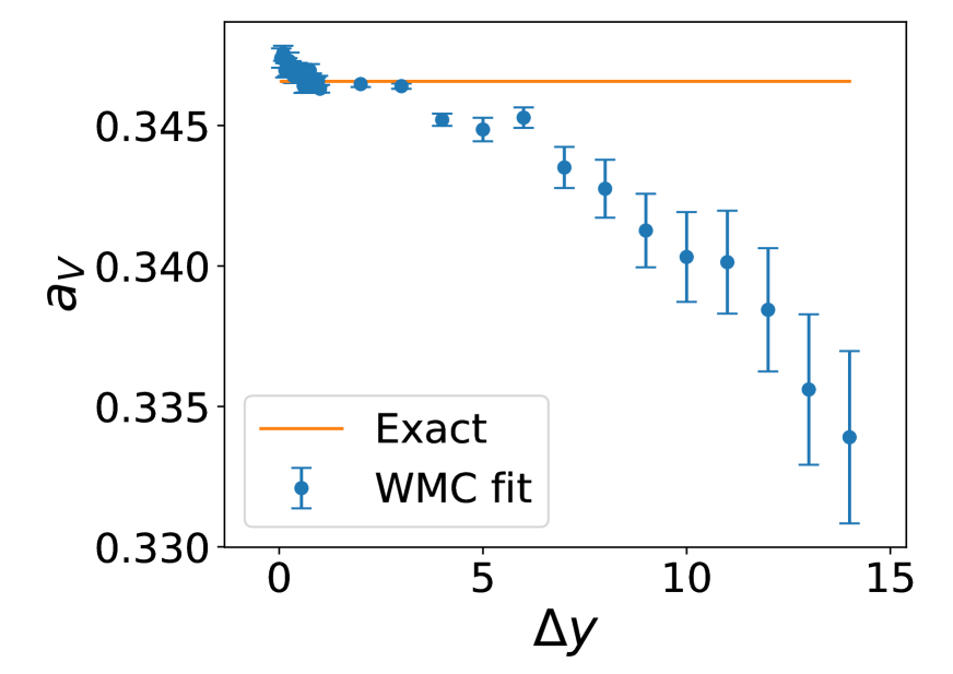
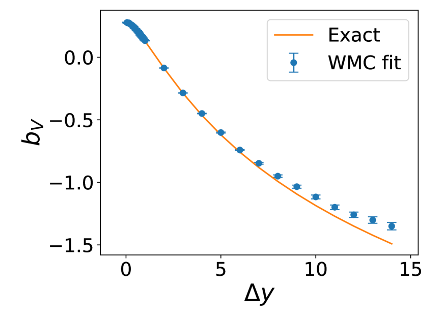
Figure 2. Fit parameters $a_{V}$ (left) and $b_{V}$ (right) of the fit eq. (27) to the expectation value of the interaction potential (light blue points), as functions of the distance $\Delta y$. The orange solid lines show the exact analytical prefactor $(\ln 2)/2$ of the log divergence (left) and the remainder function of eq. (20) after subtraction of the log-divergence (right).

4.2. Probability distribution for the interaction potential

With this validation of our numerical methods, also showing the necessity to go to large $N$ for some quantities, we now need a method to deal with expectation values of functions of the interaction potential $\left\langle f(V[x])\right\rangle_{x_{\text{I}}}^{x_{\text{F}}},$ cf. eq. (25), An obvious difficulty is the isolation of the logarithmic divergencies for increasing $N$. A naive subtraction of the analytically known divergence in eq. (25) would be problematic, as any numerical error in determining this divergence gets amplified with $\ln N$ after analytical subtraction.

In the following, we use the method of numerically determining the probability distribution of the relevant observable as introduced in [18] for the coincidence limit and generalize it to finite distances $\Delta x$. We define the distance-dependent probability distribution function (PDF) $\mathcal{P}(v,\Delta y)$ for the potential

$$\begin{split}\mathcal{P}(v,\Delta y)=\frac{\int_{y(0)=y_{\text{I}}}^{y(1)=y_{\text{F}}}\mathcal{D}y\,e^{-\int_{0}^{1}\frac{\dot{y}^{2}}{4}}\delta\left({\scriptsize\frac{1}{T}}V[y]-v\right)}{\int_{y(0)=y_{\text{I}}}^{y(1)=y_{\text{F}}}\mathcal{D}y\,e^{-\int_{0}^{1}\frac{\dot{y}^{2}}{4}}},\end{split}$$ (28)

where we have scaled out the trivial linear propertime dependence of $V[y]$, cf. eq. (13), such that $\mathcal{P}(v,\Delta y)$ is not explicitly $T$-dependent. In addition to $\Delta y$, the PDF using a discretized definition also depends on $N$. Once the PDF is known, the desired expectation value can be computed from

$$\left\langle f\left(V[y]\right)\right\rangle_{y_{I}}^{y_{F}}=\int_{0}^{\infty}dv\,\mathcal{P}(v,\Delta y)\,f(Tv).$$ (29)

In the following, we determine the PDF from numerical data, i.e., from binned histograms of the observable $V[y]$, and analyze it with a suitable fit function. For the latter, we choose

$$P(v,\Delta y):=\frac{\beta^{1+\alpha}}{\Gamma(\alpha+1)}(v-v_{0})^{\alpha}e^{-\beta(v-v_{0})}\theta(v-v_{0}),$$ (30)

where the fit parameters $\alpha$, $\beta$ and $v_{0}$ are all $\Delta y$ dependent. The fit function is already normalized, $\int_{0}^{\infty}dv\,P(v,\Delta y)=1$. Also, it has been designed in such a way that the $N$-dependent log divergence can be carried by the parameter $v_{0}$, see below.

In Fig. 3 (left panel), we depict the numerically obtained PDF $\mathcal{P}(v,\Delta y)$ using 100 bins for the case of a closed loop (coincidence limit with $\Delta y=0$) and $N=2^{5}$ points per loop.

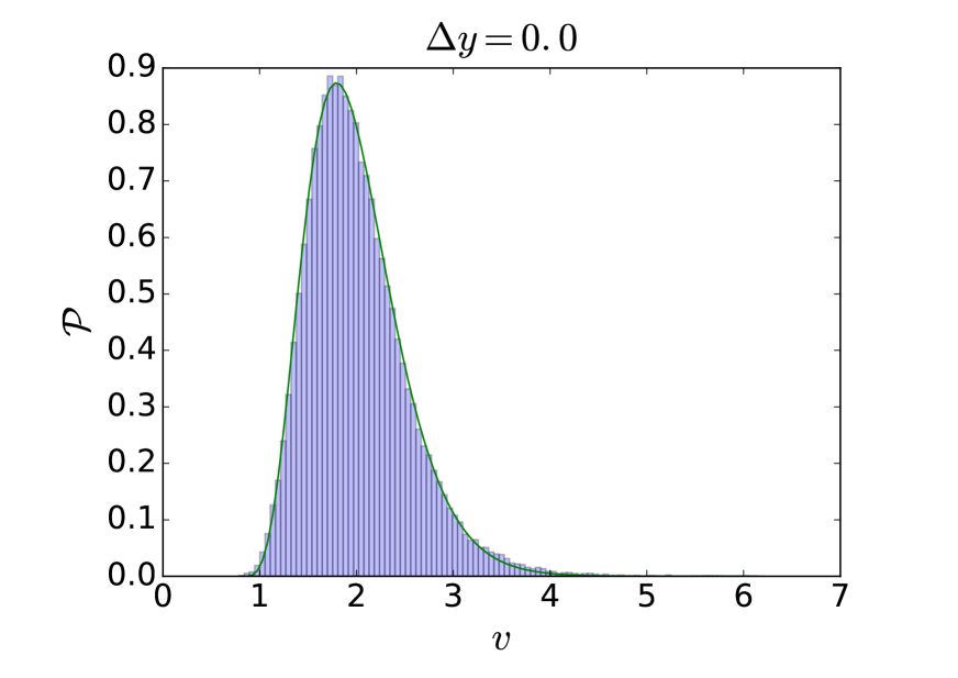
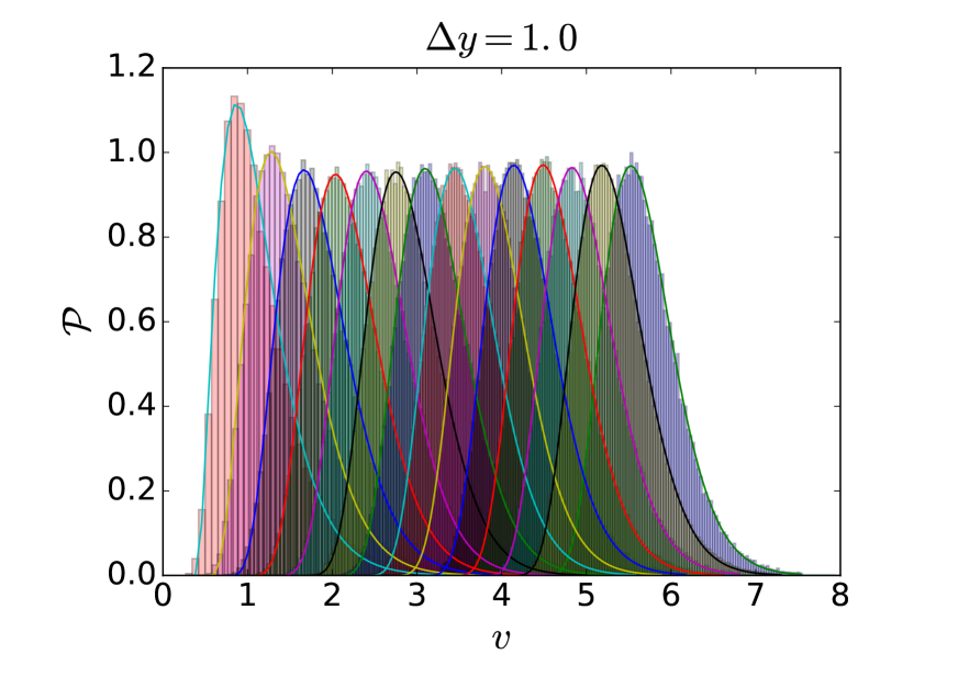
Figure 3. Probability distributions $\mathcal{P}$ and the corresponding fits $P$ for $\Delta y=0$, $N=5$ (left) and $\Delta y=1$, $N=3,4,\cdots,16$ (right), with $N$ increasing from left to right in the right plot.

The fit $P(v,0)$ according to the ansatz (30) is also shown. As is visible from the plot, the proposed fit function $P$ is compatible with the main features of the numerical data $\mathcal{P}$: its decay for large and small potential, the existence of a maximum, and the position of the latter.

On the right panel of Fig. 3, a set of these PDFs and their corresponding fits are shown for increasing values of $N=2^{k}$, $k=3,6,\dots,16$, and for finite $\Delta y=1$. We observe that the peak position shifts linearly with $k$, i.e., increases logarithmically with $N$. More importantly, the shape of the PDF approaches an asymptotic form for increasing $N$. Indeed, this can be quantified by studying the behavior of the fit parameters $\alpha$ and $\beta$ for increasing $N$, which is shown in Fig. 4 for $\Delta y=1$.

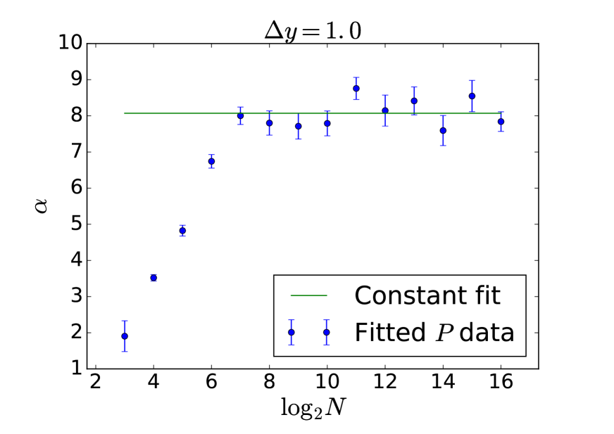
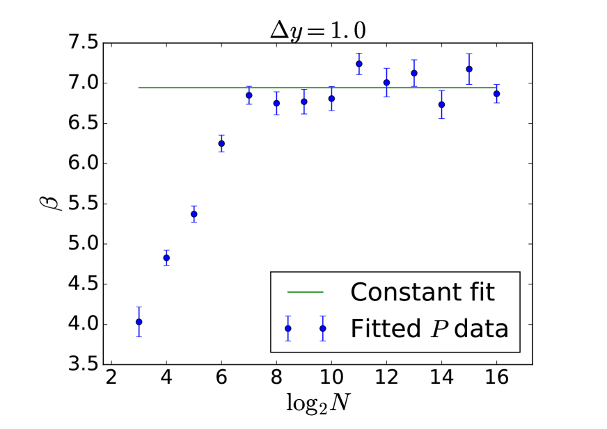
Figure 4. The $\alpha$ (left) and $\beta$ (right) parameters for $\Delta y=1$ as a function of $N$. The blue dots correspond to the data coming from the fit of our Ansatz $P(v,\Delta y)$ to $\mathcal{P}$ for different values of $N$, while the green solid line is the constant fit in the large $N$ region.

After a linear increase with $\ln N$ for small $N$, they show a convergent behavior for larger $N$, indicated by a clear flattening of the curve for increasing $N$. We extract our estimates for the asymptotic values of $\alpha$ and $\beta$ in the large N limit from a fit to a constant in that flat region. Unfortunately, the onset of that flat region depends on $\Delta y$ and occurs at larger $N$ for increasing $\Delta y$. This fact ultimately puts a limit on the accessible range of propagation distances $\Delta x$.

In order to identify the flat region where the parameters $\alpha$ and $\beta$ have settled, we may inspect the $N$ dependence by hand as in Fig. 4. Alternatively, we can use the one-loop test described at the end of Subsect. 4.1, requiring $N$ to be sufficiently large to identify the logarithmic one-loop divergence with a precision of, say, more than 90%. In practice, we find that both methods yield results for a minimum number of $N$ which agree with one another.

As mentioned above, the log-divergence in $N$ is carried by the parameter $v_{0}$. This is also obvious from the parametrization of the expectation value of the interaction potential upon using the PDF fit (30),

$$\frac{1}{T}\left\langle V[y]\right\rangle_{y_{I}}^{y_{F}}\simeq\langle v\rangle_{P}:=\int_{0}^{\infty}dv\,P(v)\,v=v_{0}+\frac{1+\alpha}{\beta}.$$ (31)

We have already worked out the $\ln N$ divergence of the left-hand side explicitly, whereas we have shown numerically that $\alpha$ and $\beta$ converge to finite values for large $N$. Hence, the parameter $v_{0}$ must behave as $v_{0}\sim(\ln N)/2$. As mentioned previously, this is in agreement with the shift of the peak of the PDF as visible in Fig. 3 (right panel) and can quantitatively be confirmed by an analysis of the fit parameter results for $v_{0}$ – see Fig. 5, left plot, where this behavior is depicted for $\Delta y=1$ together with a large $N$ fit of the form

$$f_{v_{0}-\text{fit}}=a_{v_{0}}\log_{2}N+b_{v_{0}}.$$ (32)

In the same way as for the parameters $\alpha$ and $\beta$, the choice of the large-$N$ fit region can be done by either visual inspection or using the one-loop test. Both methods provide equivalent results.

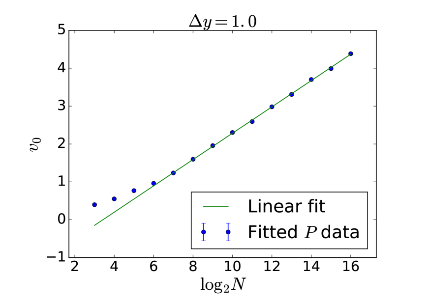
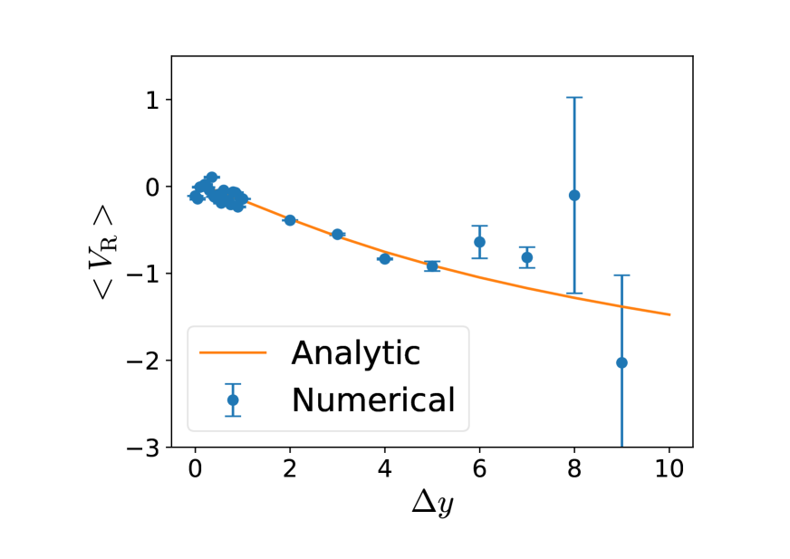
Figure 5. Left: $N$ dependence of the fit parameter $v_{0}$ for $\Delta y=1$; the blue dots show the results from fitting $P(v,\Delta y)$ to $\mathcal{P}$ for different values of $N$, and the green solid line represents the linear $\log_{2}N$ fit in the large $N$ region. Right: self-consistency check using the regularized analytical result (eq. (84), solid orange line) and the regularized numerical one (eq. (34) using the large-$N$ fit values of $\alpha$, $\beta$ and $b_{v_{0}}$, blue dots) for $T=1$.

These numerical results for $v_{0}$ are, however, not required for the following analysis. In fact, having computed $\alpha$ and $\beta$ numerically, and knowing $\left\langle V[y]\right\rangle_{y_{I}}^{y_{F}}$ analytically from eq. (20), $v_{0}$ can be determined from eq. (31),

$$v_{0}=\frac{1}{T}\left\langle V[y]\right\rangle_{y_{I}}^{y_{F}}-\frac{1+\alpha}{\beta}.$$ (33)

This is the estimator we will use for $v_{0}$ in the following sections. The advantage of this way of extracting $v_{0}$ is that the fully available analytical information for the expectation value of the interaction potential can be used. This facilitates at the same time an exact subtraction of the log-divergencies in the course of the renormalization procedure, see below.

Computing $v_{0}$ numerically from the PDF fit instead serves as a worthwhile self-consistency check: if the obtained fits are valid, the WMC estimation in formula (31) should hold true upon replacing the parameters $\alpha$, $\beta$ and $v_{0}$ by their large-$N$ asymptotic expressions, while using the analytical expression (20) for $\langle V\rangle_{y_{\text{I}}}^{y_{\text{F}}}$.

To this end, in App. C we determine the large-$N$ asymptotic expansion of (20) up to $o(N^{0})$. With this information, we can cancel the leading $\log_{2}N$ contributions on both sides of the estimation (31). The result is a “renormalized” self-interaction potential $V_{\text{R}}$. Our analytic large-$N$ result is given in eq. (84), so that the corresponding numerical estimate is given by

$$\frac{1}{T}\left\langle V_{\text{R}}[y]\right\rangle_{y_{I}}^{y_{F}}\simeq b_{v_{0}}+\frac{1+\alpha}{\beta}-\frac{\gamma}{2}.$$ (34)

It should be clear that the attribute “renormalized” is justified, as the subtraction corresponds precisely to the mass renormalization, cf. eq. (24). Note that also the finite parts are subtracted, such that $\left\langle V_{\text{R}}[y]\right\rangle_{y_{I}}^{y_{F}}\to 0$ for $\Delta y\to 0$. Results for $\left\langle V_{\text{R}}[y]\right\rangle_{y_{I}}^{y_{F}}$ are shown in the right panel of Fig. 5. This demonstrates that the fit results are indeed self-consistent up to distances of order $\Delta y\sim 5$. This serves as an indication for the region of confidence of our numerical computations. We observe that the uncertainties in the numerical data, arising from a propagation of uncertainties in the fit parameters, reflects the same limitation, inasmuch as they strongly increase for distances near $\Delta y\sim 5$.

In summary, the essential ingredient for obtaining non-perturbative information about the propagator is the determination of the PDF parameters $\alpha$ and $\beta$ as a function of the (rescaled) distance $\Delta y$. In addition to using simulational data for $\alpha$ and $\beta$ directly, we find it useful to introduce simple fit functions for their distance dependence.

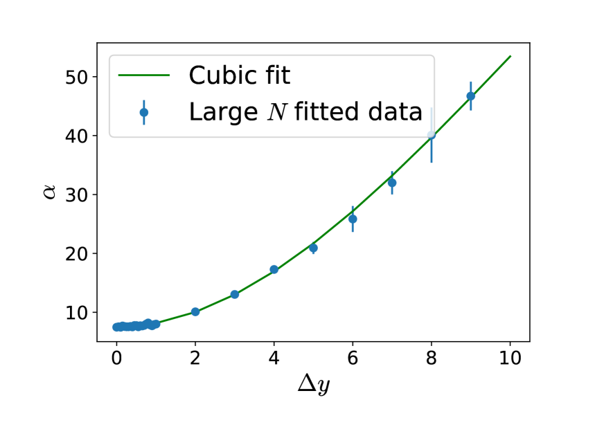
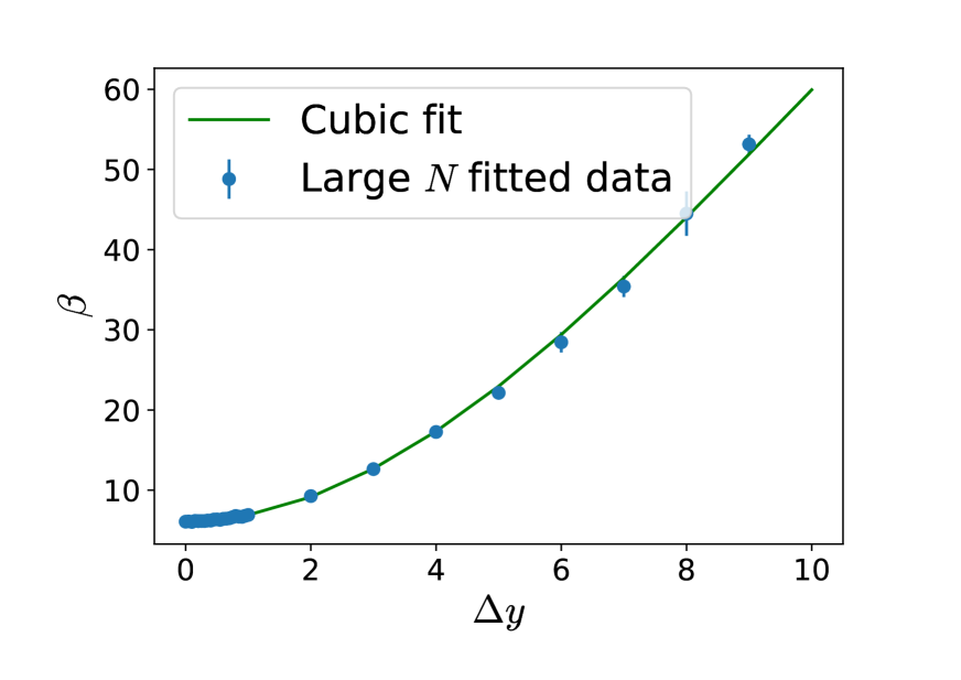
Figure 6. PDF fit parameters $\alpha$ (left) and $\beta$ (right) as a function of the distance $\Delta y$. The blue dots corresponds to the large $N$ fits of the $\alpha$ and $\beta$ parameters, while the green solid line is a third order polynomial fit.

For completeness, we consider the distance dependence of all the parameters. On the one hand, we find that both parameters $\alpha$ and $\beta$ are accurately fitted by a polynomial of third degree in the a priori determined region of confidence $\Delta y\lesssim 5$, while $a_{v_{0}}$ remains constant as predicted. The results of these fits are

$$\begin{split}\alpha&=7.5116_{8}+0.6757_{9}x^{2}-0.02164_{3}x^{3},\\ \beta&=6.1276_{2}+0.8093_{3}x^{2}-0.027124_{8}x^{3},\\ a_{v_{0}}&=0.346749_{2},\end{split}$$ (35)

as displayed in Fig. 6 for the $\alpha$ and $\beta$ parameters (left and right panel respectively), and in the left panel of Fig. 7 for the slope $a_{v_{0}}$ of $v_{0}$. The blue dots with error bars correspond to the large-$N$ asymptotic fits performed, whereas the green solid line depicts the fit functions of (35). We observe that the coefficients of the cubic terms are significantly smaller than the quadratic ones, suggesting a large radius of convergence of the polynomial expansion. Also, the fits (35) describe the data for $\alpha$ and $\beta$ well beyond the confidence region.

On the other hand, the $b_{v_{0}}$ parameter, characterizing the finite part of $v_{0}$, exhibits a non-trivial behavior encoded in eq. (84) and (34). Equation (85) in App. C suggests that a small distance fit of $b_{v_{0}}$ should require at least two parameters. Instead, in order to avoid the proliferation of parameters, we test the quality of our data by the following comparison: we start from eq. (34), solve it for $b_{v_{0}}$,

$$b_{v_{0}}=\frac{\gamma}{2}-\frac{1+\alpha}{\beta}+\frac{1}{T}\left\langle V_{\text{R}}[y]\right\rangle_{y_{I}}^{y_{F}},$$ (36)

and insert the fits (35) of $\alpha$ and $\beta$ on the right-hand side as well as the analytically determined form of the renormalized self-interaction potential, cf. eq. (84). This gives us a fully determined and analytically controlled estimator of $b_{v_{0}}$ without further parameters. We compare this result with the numerical data obtained by using the fit (32) in Fig. 7 (right). We observe a good agreement in the region of confidence $\Delta y\lesssim 5$. In fact, $b_{v_{0}}$ is the only quantity parametrizing our data, where the noise beyond the region of confidence shows up.

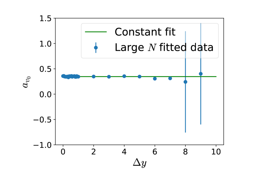
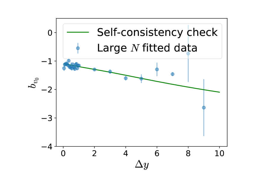
Figure 7. PDF fit parameters $a_{v_{0}}$ (left) and and $b_{v_{0}}$ (right) representing the fit parameter $v_{0}$ via eq. (32) as a function of the distance $\Delta y$. The blue dots corresponds to the large $N$ fits of the $v_{0}$ parameter. In the left panel, the green solid line is a constant fit, whereas in the rigth panel it shows the estimate for $b_{v_{0}}$ using eq. (36) as described in the text.

4.3. Results for the propagator

Let us now apply the PDF-based formalism to the worldline representation of the propagator $G(\Delta x)$ for the charged scalar written in terms of the worldline expectation value of the exponential of the potential $V$, cf. eq. (10) in Sect. 2:

$$G(\Delta x) =\frac{1}{(4\pi)^{d/2}}\int_{0}^{\infty}\frac{dT}{T^{d/2}}e^{-m_{\text{WR}}^{2}T}e^{-\frac{\Delta x^{2}}{4T}}\left\langle e^{-\delta m^{2}T-gV[y]}\right\rangle_{\frac{x_{\text{I}}}{\sqrt{T}}}^{\frac{x_{\text{F}}}{\sqrt{T}}}.$$ (37)

Using the ansatz for the PDF given by (30), it is straightforward to obtain an estimate of the expectation value in terms of the fit parameters,

$$\left\langle e^{-gV[y]}\right\rangle_{\Delta y}\simeq\left\langle e^{-gTv[y]}\right\rangle_{P,\Delta y}=F_{(\alpha(\Delta y),\beta(\Delta y))}(gT)e^{-gTv_{0}(\Delta y)},$$ (38)

where we have explicitly highlighted the dependence of the parameters on the distance $\Delta y$ and defined the auxiliary function

$$F_{(\alpha,\beta)}(gT):=\left(\frac{\beta}{\beta+gT}\right)^{1+\alpha}.$$ (39)

Inserting eq. (38) into eq. (37) leads us to

$$G(\Delta x) \simeq\frac{1}{(4\pi)^{d/2}}\int_{0}^{\infty}\frac{dT}{T^{d/2}}e^{-m_{\text{WR}}^{2}T}e^{-\frac{\Delta x^{2}}{4T}}F_{(\alpha,\beta)}(gT)e^{-gTb_{v_{0}}+\frac{g}{2}T\gamma}$$ (40)

$$=:G_{P}(\Delta x).$$ (41)

As a quick check, consider the one-loop expansion of this formula: performing a naive expansion of (40) in powers of $g$ leads to

$$G_{P}(\Delta x) =\frac{1}{(4\pi)^{d/2}}\int_{0}^{\infty}\frac{dT}{T^{d/2}}e^{-m_{\text{WR}}T}e^{-\frac{\Delta x^{2}}{4T}}\left[1-\left(b_{v_{0}}+\frac{1+\alpha}{\beta}-\frac{\gamma}{2}\right)gT+\cdots\right],$$ (42)

which together with eq. (34) tells us that this is indeed the renormalized result corresponding to a linear expansion in the potential $V$.

For a further analysis, it is useful to measure all dimensionful quantities in units of the mass scale $m_{\text{WR}}$, and introduce the dimensionless quantities

$$\bar{G}_{P}(\cdot) =\frac{1}{m_{\text{WR}}^{2}}G_{P}(\cdot),$$ (43)

$$\bar{g} =\frac{g}{m_{\text{WR}}^{2}},$$ (44)

$$\Delta\bar{x} =m_{\text{WR}}\Delta x.$$ (45)

We also perform a corresponding rescaling of the propertime T with a subsequent substitution by $T\to\Delta\bar{x}T$, yielding

$$\bar{G}_{P}(\Delta\bar{x}) =\frac{1}{(4\pi)^{2}\Delta\bar{x}^{2}}\int_{0}^{\infty}dT\,\mathcal{G}_{\Delta\bar{x},\bar{g}}(T),$$ (46)

where the rescaled propertime integrand is

$$\mathcal{G}_{\Delta\bar{x},\bar{g}}(T): =\frac{1}{T^{2}}e^{-\left(1+\bar{g}b_{v_{0}}(\frac{1}{\sqrt{T}})-\frac{\bar{g}}{2}\gamma\right)\Delta\bar{x}^{2}T}e^{-\frac{1}{4T}}F_{\left(\alpha\left(\frac{1}{\sqrt{T}}\right),\beta\left(\frac{1}{\sqrt{T}}\right)\right)}(\Delta\bar{x}^{2}\bar{g}T).$$ (47)

Formulas (46) and (47) assume that the values of the $\alpha$, $\beta$ and $b_{v_{0}}$ parameters are known for every positive argument. However, we have already determined in Sect. 4 that our region of confidence is limited to arguments $\Delta y$ satisfying $\Delta y\lesssim 5$. In the present rescaled form, this translates to propertime values $T\gtrsim 0.04$. As the propertime is an integration variable on the positive real domain, our result for the propagator can only be considered a valid estimate if the integrand $\mathcal{G}_{\Delta\bar{x},\bar{g}}(\cdot)$ is localized in propertime regions satisfying this constraint on $T>T_{\text{est}}=0.04$.

Whether this constraint is satisfied depends on the coupling parameter $\bar{g}$ and the distance $\Delta\bar{x}$ under consideration. The dominant features of the integrand arise from the interplay between two expontential terms: the first one with an exponent proportional to $T$ stems from the mass term and controls the large-$T$ behavior, also relates to the long-range properties of the propagator. The second exponential, with an exponent proportional to the inverse of T, controls the small-$T$ (short-range) behavior. As a result, the propertime integrand has a single peak, being exponentially damped to both sides of the peak. We thus consider our estimate for the propagator reliable, as long as the dominant part of the peak of the integrand is located at propertime values satisfying $T>T_{\text{est}}$.

As an example, consider the left panel of Fig. 8. Here, we plot the propertime integrand (47) as a function of the proper time $T$ for $\bar{g}=0.5$ and different values of the distance $\Delta\bar{x}$, using the numerical data; for a better comparability, we have normalized the peak of the integrand to one. Notice also that the numerical uncertainties coming from a propagation of errors in the parameter uncertainties, cf. (35) are in these cases smaller than the width of the plotted lines. As expected, the integrand is peaked aroung a value $T_{\text{max}}$ that tends to zero as the distance $\Delta\bar{x}$ increases. In this particular case, the conclusion is that our formula (46) represents a satisfactory estimate up to distances of order one. As a way to quantify the systematic error of our method when computing the propagator, we assign an uncertainty given by the value of an integral analogous to (46) with the upper boundary replaced by the value 0.04. We believe that this procedure yields rather conservative error bars.

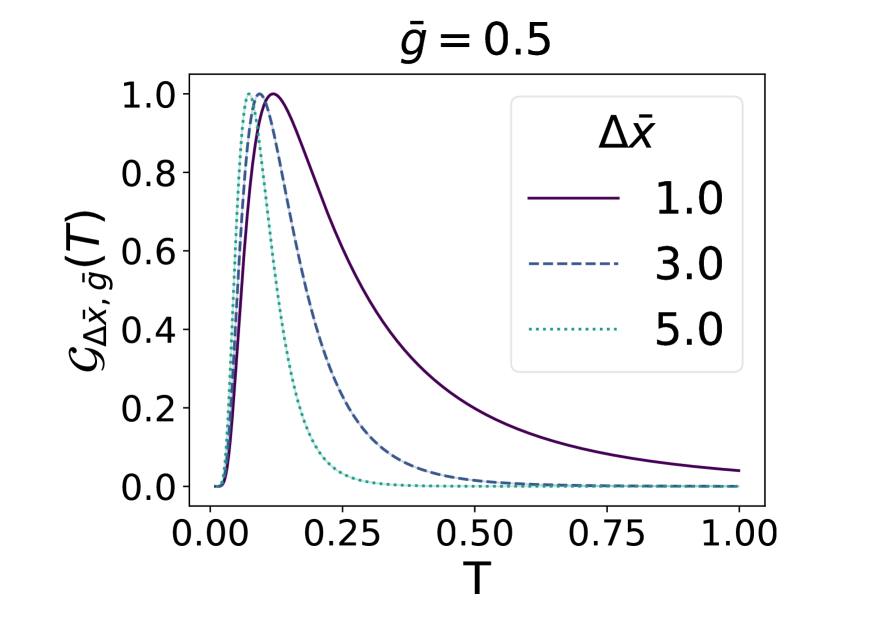
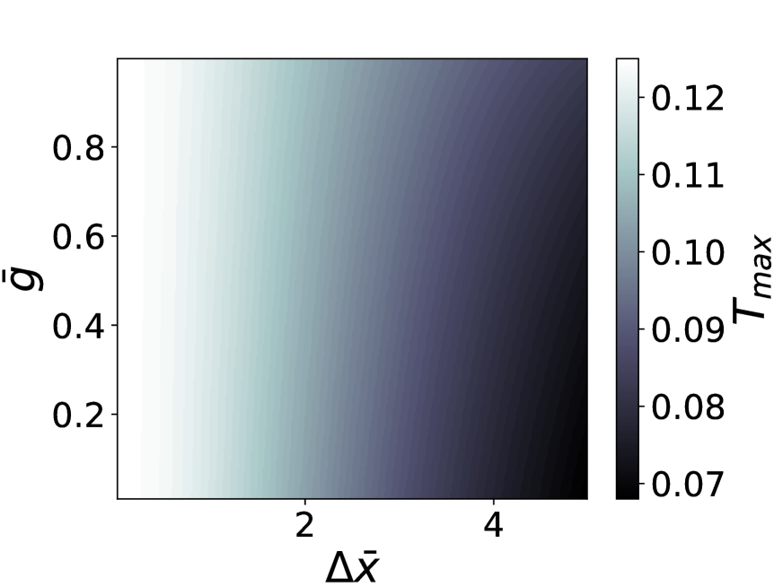
Figure 8. Left: peak-normalized integrand $\mathcal{G}$ of eq. (47), for $\bar{g}=0.5$ and distances $\Delta\bar{x}=1,3,5$ (solid violet, dashed blue and dotted cyan lines respectively). Right: density plot of the propertime peak position $T_{\text{max}}$ of $\mathcal{G}$ as a function of $\bar{g}$ and $\Delta\bar{x}$.

Additionally, we show in Figure 8 (right) a density plot of the peak position $T_{\text{max}}$ of $\mathcal{G}_{\Delta\bar{x},\bar{g}}$ as a function of the dimensionless distance $\Delta\bar{x}$ and coupling $\bar{g}$. Obviously, the region of self-consistency $T_{\text{max}}>T_{\text{est}}=0.04$ corresponds to small values of $\Delta\bar{x}$; we observe hardly any restriction on the coupling $\bar{g}$ in its allowed region.

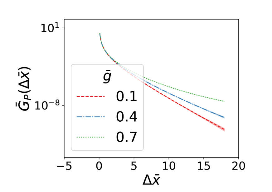
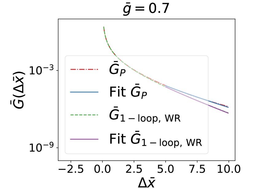
Figure 9. Left panel: behaviour of the propagator $\bar{G}_{P}(\cdot)$ as a function of the distance for $\bar{g}=0.1$ (dashed red line), $\bar{g}=0.4$ (dot-dahed blue line) and $\bar{g}=0.7$ (dotted green line). Right panel: propagator (dot-dashed red line) and the one-loop propagator $G_{1-\rm{loop},\,WR}$ in the worldline regularization (dashed green line) together with their large distance fits (solid blue and violet line, for the full and one-loop propagator, respectively).

In fact, the region where we consider (47) to be valid is limited by the constraint that the first exponential factor remains decaying for large $T$. This leads to a constraint on the coupling:

$$1+\bar{g}b_{v_{0}}(0)-\bar{g}\frac{\gamma}{2}>0\quad\Longrightarrow\quad\bar{g}<\bar{g}_{\text{c}}\simeq 0.72.$$ (48)

For couplings stronger than the critical one, the integrand (47) becomes divergent for large propertimes. The maximum displayed on the right panel of Fig. 8 therefore becomes only a local one beyond the critical coupling.

Taken at face value, the limiting value $g=g_{\text{c}}$ corresponds to a coupling strength, where the propagator no longer decays exponentially for large distances, i.e. where the physical mass appears to tend to zero. At least in the present approximation, we are lead to conclude that the initially massive particle can become massless because of the dressing through the photon cloud if the coupling approaches the critical value. Whether this remains a feature of the model beyond our approximation is difficult to estimate, since it requires a careful study of the long-distance limit of the propagator.

This can be appreciated in the left panel of Fig. 9, where the propagator is plotted as a function of the distance $\Delta\bar{x}$ for several values of the coupling. The exponential decay is indeed softened as the coupling increases. In the right panel of Fig. 9 we include, for $\bar{g}=0.7$, the comparison between the propagator and the one-loop propagator $G_{\text{1-loop, WR}}$ in the worldline regularization (cf. eq. (93) and in general App. D for its definition). Note that for large distances both of them decay exponentially as the free propagator given by expression (11) does. For this reason we propose the following fit function for the propagators in the large distance regime,

$$f(x)=\frac{A}{x^{3/2}}e^{-m^{\star}x},$$ (49)

where $A$ and $m^{\star}$, i.e. the physical mass corresponding to the pole mass, are the fit parameters.

Remarkably, the fits are in excellent agreement with the propagators for $x$ larger than unity, as can be seen in the right panel of Fig. 9: the blue (violet) solid line corresponds to the fit of the propagator $\bar{G}_{P}$ ($G_{\text{1-\rm{loop}, WR}}$). Contrary to the free case, the physical mass in the interacting case is not equal to the scale-setting mass $m_{\text{WR}}$, which is taken as unity in these plots. Rephrasing this, in the light of the results (90) and (93), it is clear that the scale-setting mass $m_{\text{WR}}$ does in general not coincide with the pole mass $m^{\star}$ of the propagator in complex momentum space.

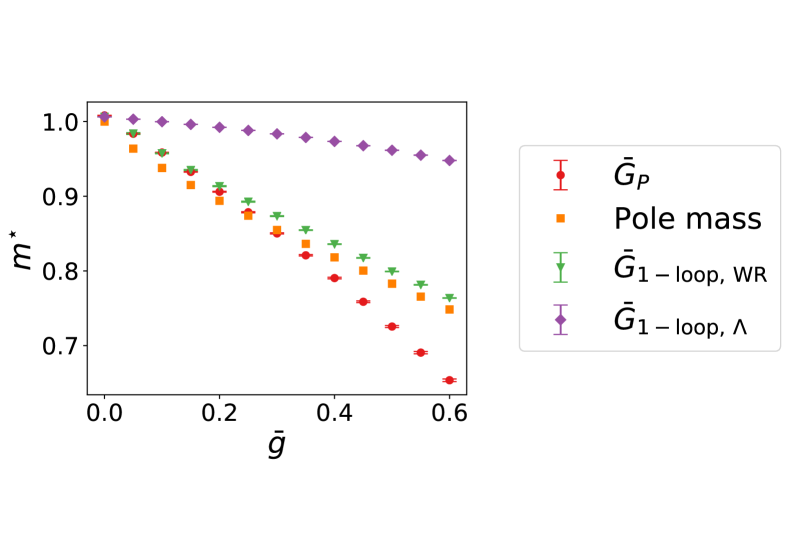
Figure 10. Pole mass $m^{\star}$ as a function of the coupling constant for various estimates: within worldline regularization, the analytical one-loop result is shown as orange squares, exhibiting satisfactory agreement with the same result extracted from a fit procedure (green triangles). The nonperturbative worldline result using the same fit procedure is shown as red circles. For comparison, we show the one-loop pole mass extracted from the propagator using cutoff regularization (purple diamonds).

Performing the analysis of physical masses for a wide range of coupling values, we summarize our findings in Fig. 10. As a first benchmark, we plot the pole mass $m^{\star}$ as extracted from the asymptotic expansion of the one-loop propagator within the worldline regularization, cf. App. E, as orange squares. Since our numerical data does not permit to go to asymptotically large distances, we need to perform the numerical fits in a window of finite $x$ values (we use $5\lesssim x\lesssim 10$). Applying this procedure to the one-loop worldline result, we obtain the data points shown as green triangles. Over the full range of couplings, this estimate is satisfactorily close to the analytical result for the pole mass with deviations due to the fit procedure on the few percent level.

We consider the smallness of these deviations as indicative for the reliability of the fit procedure for the full propagator, whose results are shown as red circles. A direct observation shows that the one-loop approximation is quantitatively accurate up to $\bar{g}\lesssim 0.2$. For larger couplings, our estimate for the pole mass of the propagator decreases more rapidly than the one-loop estimate. We interpret this as a consequence of the dressing of the charged particle with the (scalar) photon cloud, which is described by the infinite subclass of Feynman diagrams resummed by the nonperturbative worldline formula (10). As discussed above, the charged particle even becomes massless for $\bar{g}\to\bar{g}_{\text{c}}\simeq 0.72$.

For further comparison, we also show the pole mass as derived from the one-loop propagator using a momentum cutoff regularization ($\bar{G}_{1-\rm{loop},\,\Lambda}$, purple diamonds). The qualitative trend of a decreasing pole mass for increasing couplings is also visible. However, the dependence on the coupling appears much weaker. As emphasized above and explained in more detail in App. D, the difference arises from the use of very different regularization methods. Correspondingly, we expect the critical coupling $g_{\text{c}}$ to be non-universal, i.e. to depend on the regularization scheme. Nevertheless, the trend of the nonperturbative fluctuations to lower the pole mass for larger couplings should persist in any regularization scheme.

Finally, we observe that the propagator in the deep UV region remains unaffected by the fluctuations. For $\Delta\bar{x}\ll 1$, the behavior of both the one-loop propagator $G_{1-\rm{loop},\,WR}$ and the propagator $\bar{G}_{P}$ coincide with that of the free propagator $\bar{G}_{0}$. This can be deduced from the analytical expressions (46) and (93) by expanding for small $\Delta\bar{x}$,

$$\bar{G}_{1-\rm{loop},\,WR}(\Delta x)\sim\bar{G}_{P}(\Delta x)\sim\frac{1}{4\pi^{2}\Delta x^{2}},\qquad\Delta x\ll 1,$$ (50)

and is also confirmed by our numerical results. This observation is also in line with the superrenormalizability of the model: the only possible divergence is related to the mass operator – UV-fluctuations are not strong enough to also give rise to anomalous dimensions which could have modified the short distance behavior given in formula (50).

5. Conclusions

We have extended nonperturbative worldline methods to a computation of a full propagator in S²QED, a two-scalar model with cubic interaction. For this, we have combined a compact worldline representation for a large subclass of Feynman diagrams with information carried by the probability distribution function of a relevant worldline observable. This has enabled us to perform the renormalization of the model nonperturbatively and to compute the propagator of the scalar electron for large values of the coupling beyond the perturbative validity region.

The fully resummed subclass of diagrams is the dominant set in the formal small flavor $N_{\text{f}}\to 0$ limit. For the scalar electron propagator, it diagrammatically corresponds to the electron line dressed by all possible photon radiative corrections but without any additional electron loop. The computation becomes accessible in the worldline formalism as it corresponds to an expectation value of a worldline observable which we have been able to compute using the method of probability distribution functions. Algorithmically, we have followed corresponding earlier suggestions for effective action computations [18] and generalizing these methods for propagators on the basis of a newly developed $v$ lines algorithm, cf. App. A. These methods result in a semi-analytical expression for the propagator, i.e. an analytical form that depends on a few parameters to be determined from worldline simulations. Once the parameters are computed numerically, the analysis of the propagator can be performed largely analytically.

This gives rise to a number of concrete results for the model: as a general aspect, we observe that the propagator is always positive for the range of accessible coupling values, so that we observe no violation of reflection positivity. More precisely, we have analyzed the dependence of the propagator on the distance as a function of the coupling. The large distance behavior is governed by the physical (pole) mass corresponding to the inverse correlation length characterizing the propagator.

For small couplings, our nonperturbative results coincide with that of the one-loop approximation given by the resummation of the lowest-order self-energy diagrams. Even though asymptotically large distances are numerically difficult to deal with, the accessible distances already exhibit the expected asymptotic behavior and allow for a determination of the pole mass for comparatively large couplings $\bar{g}\sim 0.5$.

From about $\bar{g}\sim 0.2$ on, we observe a clear deviation from the perturbative estimate indicating the onset of a nonperturbative domain. The inclusion of more diagrams corresponding to a full radiative dressing of the electron with a photon cloud reduces the physical pole mass compared to the leading-order perturbative estimate. Our results are compatible with the existence of a critical coupling value for which the physical mass approaches zero as a consequence of the radiative dressing. This result agrees with the fact that our semi-analytical expression (47) shows a constraint on the coupling parameter given by (48), which can be interpreted as an estimate of the critical coupling.

For these results, we have used a specific regularization prescription which arises naturally in the worldline formalism in the form of a discretization of dimensionless worldline trajectories in terms of polygons of $N$ segments. While this worldline regularization of keeping $N$ finite is simple and straightforward to use in analytical as well as numerical worldline computations, the relation to conventional regularizations of Feynman diagrams is more involved. This is already obvious from the fact that the dimensionless parameter $N$ needs to be related to a dimensionful parameter (such as a UV cutoff $\Lambda$ or a renormalization scale $\mu$) which requires the dimensionality to be balanced by the physical momentum or distance scale (at least in the deep Euclidean region). As a consequence, our worldline result for the propagator determined with our regularization differs from those of standard regularizations by computable logarithmic terms. Such regularization dependences correspondingly occur for all non-universal quantities such as the critical coupling value where the mass vanishes. Still, the existence of a critical coupling is also suggested by the behavior of the propagator in standard regularization schemes.

Finally, we observe that the small-distances behaviour of the propagator is not affected by photonic corrections, neither perturbatively nor in the nonperturbatve worldline computation. We consider this as evidence that the superrenormalizable structure of the theory as suggested by power-counting is preserved also nonperturbatively. As a result, the anomalous dimension of the scalar electron field in S²QED remains zero both in perturbation theory and beyond.

Appendix A The $v$-lines algorithm

In the following, we construct an algorithm that generates open worldlines that obey a Gaußian velocity distribution. This $v$ lines algorithm is a generalization of the efficient $v$ loops algorithm introduced in [48] which generates corresponding closed worldlines. Open worldlines can also efficiently be generated by a variant of the $d$ loop algorithm [18] that also works for open lines [58, 59], however, the following $v$ lines algorithm can be employed for an arbitrary number of points (for $d$ lines or loops they always come in powers of 2).

First of all, we intend to create an ensemble of lines that run from $y_{0}$ to $y_{N}$ in $D$ dimensions according to the discretized Gaussian velocity distribution

$$\begin{split}\bar{\mathcal{N}}\int_{y_{0}}^{y_{N}}\mathcal{D}y\,e^{-\frac{N}{4}\,S_{W}[y]}:=\bar{\mathcal{N}}\int\prod_{j=1}^{N-1}d^{D}y_{j}\,e^{-\frac{N}{4}\sum_{i=1}^{N}(y_{i}-y_{i-1})^{2}},\end{split}$$ (51)

where $\bar{\mathcal{N}}$ is the normalization needed to have a normalized-to-one distribution. The idea is to perform a set of linear variable transformations such that the probability distribution becomes a Gaußian one. As a first step we complete the squares for $y_{1}$:

$$S_{W}=2\left(y_{1}-\frac{y_{0}+y_{2}}{2}\right)^{2}+\frac{1}{2}(y_{2}^{2}+y_{0}^{2})-y_{0}\,y_{2}+\sum_{i=3}^{N}(y_{i}-y_{i-1})^{2}.$$ (52)

This naturally suggests to introduce a new variable $z_{1}$ defined by

$$z_{1}:=y_{1}-\frac{y_{0}+y_{2}}{2},$$ (53)

encoding all $y_{1}$ dependence of $Y$. The same procedure can be applied to the dependence of the exponent on $y_{2}$:

$$S_{W} =2\,z_{1}^{2}+\frac{3}{2}\left(y_{2}-\frac{y_{0}+2\,y_{3}}{3}\right)^{2}+\frac{1}{3}(y_{3}^{2}+y_{0}^{2})-\frac{2}{3}y_{0}\,y_{3}+\sum_{i=4}^{N}(y_{i}-y_{i-1})^{2}.$$ (54)

In this case, we obtain a purely quadratic dependence by introducing the new variable $z_{2}$,

$$z_{2}:=y_{2}-\frac{y_{0}+2\,y_{3}}{3}.$$ (55)

The general pattern for completing the squares for the $i$th variable $y_{i}$ is an expression of the form

$$a_{i}y_{i}^{2}-2y_{i}(y_{i+1}+b_{i}y_{0})=a_{i}\left(y_{i}-\frac{y_{i+1}+b_{i}y_{0}}{a_{i}}\right)^{2}-\frac{(y_{i+1}+b_{i}y_{0})^{2}}{a_{i}},$$ (56)

with coefficients $a_{i}$ and $b_{i}$. After defining the variable $z_{i}$, we are left with the following $y_{i+1}$-dependent contributions:

$$\left(2-\frac{1}{a_{i}}\right)y_{i+1}^{2}-2y_{i+1}\left(y_{i+2}+\frac{b_{i}}{a_{i}}y_{0}\right).$$ (57)

Consequently, the coefficients $a_{i}$ and $b_{i}$ are sequences that satisfy a system of recursion relations,

$$\left\{\begin{array}[]{rll}a_{i+1}&=2-\frac{1}{a_{i}},&a_{1}=2,\\ b_{i+1}&=\frac{b_{i}}{a_{i}},&b_{1}=1.\end{array}\right.$$ (60)

The solution to these recursion relations can be straightforwardly obtained,

$$\left\{a_{i}=\frac{i+1}{i},\quad b_{i}=\frac{1}{i}\right\},$$ (61)

and hence, the general form of the variable $z_{i}$ reads

$$z_{i}=y_{i}-\frac{y_{0}}{i+1}-\frac{i}{i+1}y_{i+1}.$$ (62)

The quadratic form $Y$ rewritten in terms of these new $z_{i}$ variables is finally diagonalized:

$$S_{W}=\sum_{i=1}^{N-1}\frac{i+1}{i}\,z_{i}^{2}+c\,y_{0}^{2}+d\,y_{N}^{2}.$$ (63)

The values of the numbers $c$ and $d$, as well as the constant Jacobian resulting from the change of variables $y_{i}\to z_{i}$ are not relevant when computing expectation values, since they cancel with the contributions coming from the corresponding normalization. Therefore we are left with the task to generate a Gaußian probability distribution for the variables $z_{i}$, what is straightforward, e.g., with the Box-Müller method.

In summary, the generation of $v$ lines with end points $y_{0}$ and $y_{N}$, and $N-1$ intermediate points obeying a Gaußian velocity distribution can be performed as follows:

1. generate $N-1$ numbers $w_{i},\,i=1\,\ldots,\,N-1$ via the Box-Müller method in such a way that they are distributed according to $e^{-w_{i}^{2}}$,

2. normalize the $w_{i}$, obtaining thus the auxiliary variables $z_{i}$:

   $$z_{i}=\sqrt{\frac{4}{N}}\sqrt{\frac{i}{i+1}}\,w_{i};$$ (64)

3. compute the points $y_{i}$ of the $v$ line for $i=N-1,\ldots,1$ by means of the recursive formula

   $$y_{i}=z_{i}+\frac{1}{i+1}y_{0}+\frac{i}{i+1}y_{i+1}.$$ (65)

For the special case of $y_{0}=y_{N}$, the algorithm generates closed $v$ loops attached at $y_{0}$ (so-called common point loops), which can be transformed into common center-of-mass loops by a simple translation.

A.1. Test of the $v$ lines algorithm

As a way to test the code developed for the $v$ lines, we consider a simple model in which analytical expressions can be obtained. Consider then a probability distribution $P[y]$ for a discretized path $y$ in a $D$-dimensional space given by the “action” $S_{W}[y]$ in eq. (51), i.e.

$$\begin{split}P[y]=\bar{\mathcal{N}}e^{-S_{W}[y]}.\end{split}$$ (66)

Introducing an auxiliary variable $\kappa$ as a multiplicative factor in front of the action, we can straightforwardly compute expectation values of powers of the action, for example

$$\begin{split}\left\langle S_{W}\right\rangle&=\bar{\mathcal{N}}\int dy_{1}\cdots dy_{N-1}S_{W}[y]e^{-S_{W}[y]}\\ &=\bar{\mathcal{N}}\int dy_{1}\cdots dy_{N-1}\left.\frac{de^{-\kappa S_{W}[y]}}{d\kappa}\right|_{\kappa=1}\\ &=\frac{1}{2}(N-1)D+\frac{1}{4}\Delta y^{2}.\end{split}$$ (67)

Analogously, we can also compute the root mean square (RMS) of the action

$$\sqrt{\sigma^{2}(S_{W})}=\sqrt{\left\langle S_{W}^{2}\right\rangle-\left\langle S_{W}\right\rangle^{2}}=\sqrt{\frac{(N-1)D}{2}}.$$ (68)

For the interested reader, the detailed computations can be followed in [18].

Analytical results are compared to the corresponding numerical ones for the mean value of the action $S_{W}$ together with an error given by the RMS in Table 1 for several values of $N$ and distances $\Delta y=y_{\text{F}}-y_{\text{I}}$; here, we have chosen an ensemble of $10^{4}$ lines and $D=4$. As can be seen, the relative difference of these two values,

$$\frac{\Delta S_{W}}{S_{W}}:=\frac{\left\langle S_{W}\right\rangle-\left\langle S_{W}\right\rangle_{\text{num}}}{\left\langle S_{W}\right\rangle},$$ (69)

remains smaller than the percent level even for a comparatively small number of points per line as $N=32$. Moreover, we see that also their RMSs are similar, and overstimate the difference between the numerical and the analytical results in every case.

Table 1. Mean value of the action $S_{W}$, employing both the analytical result ($\left\langle S_{W}\right\rangle$) and the numerical computation involving the $v$ lines algorithm ($\left\langle S_{W}\right\rangle_{\text{num}}$), for different values of points per line $N$ and distances $\Delta y$, employing an ensemble of $10^{4}$ lines and $D=4$. Their relative difference $\Delta S_{W}/S_{W}$ is also shown.

N	$\Delta y$	$\left\langle S_{W}\right\rangle_{\text{num}}$	$\left\langle S_{W}\right\rangle$	$\Delta S_{W}/S_{W}(\%)$
32	1	$62.17_{7.96}$	$62.25_{7.87}$	0.1
256	1	$510.08_{23.5}$	$510.25_{22.6}$	0.03
2048	1	$4094.66_{86}$	$4094.25_{64}$	-0.01
256	10	$535.14_{23.5}$	$535.25_{22.6}$	-0.03
2048	10	$4117.55_{86}$	$4119_{64}$	0.03

As a next step we consider the probability distribution function $\mathcal{P}(S^{\prime}_{W})$ for the action $S_{W}$,

$$\begin{split}\mathcal{P}(S^{\prime}_{W})&=\bar{\mathcal{N}}\int dy_{1}\cdots dy_{N-1}\delta(S_{W}-S_{W}^{\prime})e^{-S_{W}}\\ &=\mathcal{\bar{N}}(S^{\prime}_{W}-S_{\text{class}})^{-1+\frac{(N+1)D}{2}}e^{-(S^{\prime}_{W}-S_{\text{class}})}\theta(S^{\prime}_{w}-S_{\text{class}}),\end{split}$$ (70)

where the classical value for the action $S_{\text{class}}$ is given by

$$S_{\text{class}}=\Delta y^{2}.$$ (71)

The agreement between expression (70) and the numerical data is remarkable even for an ensemble of just $10^{4}$ lines. This can be seen from the histogram with 100 bins for $\Delta y=10$, $D=4$ and $N=2^{5}$, depicted in Fig. 11 as violet rectangles, and the corresponding analytic expression (solid green line).

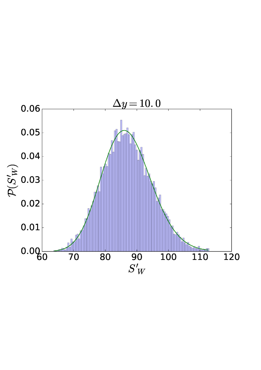
Figure 11. Probability distribution function for the action $S_{W}$ considering $\Delta y=10$, $D=4$ and $N=2^{5}$. The histogram contains 100 bins and corresponds to an ensemble of $10^{4}$ lines, whereas the solid green line is given by eq. (70).

Appendix B One-loop contribution to the propagator in the discretized formulation

As stated in Sect. 3, in order to obtain a closed expression for the mean value of the potential, we consider the Fourier transform of the interaction kernel

$$\left\langle V[y]\right\rangle^{y_{N}}_{y_{0}}=\frac{8T^{3-D/2}}{N^{2}\Gamma\left(\frac{D-2}{2}\right)}\sum_{0=l<m}^{N-1}\mathcal{N}\int_{y_{0}}^{y_{N}}\mathcal{D}y\,e^{-\frac{N}{4}\sum_{j}(y_{j}-y_{j-1})^{2}}\int\frac{d^{D}p}{(4\pi)^{D/2}}\frac{e^{ip(y_{l}-y_{m})}}{p^{2}},$$ (72)

which is evidently of Gaußian form and is valid for $D>2$. At this point, the method used in App. A to diagonalize the quadratic form in the $v$ lines algorithm can be mutatis mutandis employed. Indeed, let us inspect the quadratic form

$$Y=\sum_{j=1}^{N}\,(y_{j}-y_{j-1})^{2}-\frac{4i}{N}\,p\,(y_{l}-y_{m}).$$ (73)

Up to the ${(l-1)}$-th variable, the change of basis to the $z_{j}$ used before does the trick to diagonalize the quadratic form in the exponent, i.e.,

$$z_{j}=y_{j}-\frac{y_{0}}{j+1}-\frac{j}{j+1}y_{j+1},\quad 0<j<l.$$ (74)

The next term, however, receives an extra contribution coming from the interaction kernel so that by completing the square for $y_{l}$ we obtain the contribution

$$a_{l}\left(y_{l}-\frac{b_{l}\,y_{0}+2ip/N+y_{l+1}}{a_{l}}\right)^{2}-\frac{(b_{l}\,y_{0}+2ip/N+y_{l+1})^{2}}{a_{l}}.$$ (75)

In turn, this implies that the structure of the remaining terms in the quadratic expression (73) for $y_{j}$ is of the form

$$a_{j}y_{j}^{2}-2y_{j}\left(y_{j+1}+c_{j}\,\alpha_{0}\right),$$ (76)

where we have restricted ourselves to $l<j<m$ and defined a shifted initial position $\alpha_{0}:=b_{l}y_{0}+2ip/N$. Consequently we are left with a pair of recursion relations analogous to (60) with $c_{j}$ taking the rôle of the $b_{j}$, except for the fact that the initial condition is $c_{l}=1$. In other words, the initial condition corresponds in this case to a condition on the coefficients where the first potential insertion occurs. The diagonalizing variables are thus

$$z_{j}=y_{j}-\frac{l}{j+1}\alpha_{0}-\frac{j}{j+1}y_{j+1}\text{, for }l\leq j<m.$$ (77)

The diagonalization proceeds analogously for the variables between the second insertion of the potential and the end of the line. The result is

$$z_{j}=y_{j}-\frac{l}{j+1}\beta_{0}-\frac{j}{j+1}y_{j+1}\text{, for }m\leq j<N-1,$$ (78)

with the shifted initial position $\beta_{0}:=\frac{l}{m}\alpha_{0}-\frac{2ip}{N}$.

Although the dependence of the quadratic form on the integrating variables $z_{j}$ is the same as in the free case, we are left with an extra factor coming from the completion of the squares which depends on the insertion points ($l$, $m$) of the potential and on the end points of the line. Notice also that the Jacobian for the change of variables $y_{j}\rightarrow z_{j}$ does not get modified, since the $z_{j}$ variables are only translated with respect to the ones defined in the free case. Ergo, the normalized expression is independent both of the Jacobian and of the determinant coming from the integration over the $z$ variables:

$$\begin{split}\left\langle V[y]\right\rangle^{y_{\text{F}}}_{y_{\text{I}}}&=\frac{8\,T^{3-D/2}}{N^{2}\Gamma\left(\frac{D-2}{2}\right)}\sum_{m=1}^{N-1}\sum_{l=0}^{m-1}\int\frac{d^{D}p}{(4\pi)^{D/2}}\frac{1}{p^{2}}e^{-p^{2}\frac{(m-l)}{N}\left(1-\frac{(m-l)}{N}\right)-i\frac{(m-l)}{N}p(y_{\text{F}}-y_{\text{I}})}.\end{split}$$ (79)

Notice that this expression depends only on the relative position $(m-l)$ of the insertions, which could be understood as an inherited symmetry of paths “translations” in the continuum worldline expression.

After performing the redefinition $(m-l)\rightarrow n$ of the summation index, we find the desired expression (19), exhibited in Sect. 3:

$$\left\langle V[y]\right\rangle^{y_{\text{F}}}_{y_{\text{I}}} = \frac{8\,T^{3-D/2}}{N^{2}\Gamma\left(\frac{D-2}{2}\right)}\sum_{n=1}^{N-1}(N-n)\int\frac{d^{D}p}{(4\pi)^{D/2}}\frac{1}{p^{2}}e^{-p^{2}\frac{n}{N}\left(1-\frac{n}{N}\right)-i\frac{n}{N}p(y_{\text{F}}-y_{\text{I}})}$$ (80)

$$= 2\frac{T^{3-D/2}}{(\Delta y)^{D-2}}\sum_{n=1}^{N-1}\frac{N^{D-4}(N-n)}{n^{D-2}}\left[1-\frac{\Gamma\left(\frac{D-2}{2},\frac{n\Delta y^{2}}{4(N-n)}\right)}{\Gamma\left(\frac{D-2}{2}\right)}\right].$$

Appendix C The large-$N$ asymptotics of the discretized $\langle V\rangle_{y_{\text{I}}}^{y_{\text{F}}}$

Recall that according to expression (20) the mean value $\langle V\rangle_{y_{\text{I}}}^{y_{\text{F}}}$ of the potential in the discretized wordline regularization in $D=4$ is given by

$$\left\langle V[y]\right\rangle^{y_{\text{F}}}_{y_{\text{I}}} = 2\frac{T}{\Delta y^{2}}\sum_{n=1}^{N-1}\frac{(N-n)}{n^{2}}\left[1-e^{-\frac{n\Delta y^{2}}{4(N-n)}}\right].$$ (81)

In order to extract the large $N$ asymptotics out of this expression, we recast it in the following way:

$$\left\langle V[y]\right\rangle^{y_{\text{F}}}_{y_{\text{I}}} = 2\frac{T}{\Delta y^{2}}\sum_{n=1}^{N-1}\frac{(N-n)}{n^{2}}\left[1-e^{-\frac{n\Delta y^{2}}{4(N-n)}}-\frac{n\Delta y^{2}}{4(N-n)}+\frac{n\Delta y^{2}}{4(N-n)}\right].$$ (82)

The reason for this is that the sum of the last term can be explicitly computed as

$$2\frac{T}{\Delta y^{2}}\sum_{n=1}^{N-1}\frac{(N-n)}{n^{2}}\frac{n\Delta y^{2}}{4(N-n)}=\frac{1}{2}T\left(\log N+\gamma\right).$$ (83)

On the other hand, it can be shown that the sum running over the first three terms can be replaced by an integral in the large-$N$ limit,

$$\begin{split}\left\langle V_{\text{R}}[y]\right\rangle_{y_{\text{I}}}^{y_{\text{F}}}:&=2\frac{T}{\Delta y^{2}}\int_{0}^{1}dn\frac{(1-n)}{n^{2}}\left[1-e^{-\frac{n\Delta y^{2}}{4(1-n)}}-\frac{n\Delta y^{2}}{4(1-n)}\right]\\ &=2\frac{T}{\Delta y^{2}}\int^{\infty}_{0}\frac{dz}{z^{2}(1+z)}\left(1-\frac{z\Delta y^{2}}{4}-e^{-\frac{\Delta y^{2}z}{4}}\right)\\ &=\frac{T}{2\Delta y^{2}}\left[4e^{\frac{\Delta y^{2}}{4}}\text{Ei}\left(-\frac{\Delta y^{2}}{4}\right)+\Delta y^{2}-\left(\Delta y^{2}+4\right)\left(\gamma+\log\left(\frac{\Delta y^{2}}{4}\right)\right)\right].\end{split}$$ (84)

This is what we call the renormalized mean value of the potential $\left\langle V_{\text{R}}[x]\right\rangle_{y_{\text{I}}}^{y_{\text{F}}}$. From this expression, we can derive both a large and small $\Delta y$ asymptotics, reading

$$\left\langle V_{\text{R}}[y]\right\rangle_{y_{\text{I}}}^{y_{\text{F}}} =\begin{cases}\frac{T\Delta y^{2}}{32}\big{(}4\log\Delta y+2\gamma-3-4\log 2\big{)}+\mathcal{O}(\Delta y^{3}),&\Delta y\ll 1\\[5.69046pt] T\left(-\log\Delta y-\frac{\gamma}{2}+\frac{1}{2}+\log 2\right)+\mathcal{O}(\Delta y^{-1}),&\Delta y\gg 1\end{cases}.$$ (85)

Appendix D Self-energy for the $\phi$ field

In this appendix, we show how the worldline regularization and a cut-off regularization are related. First of all, recall that the one-loop propagator $G_{1-\rm{loop}}(x)$ may be expressed in terms of the self-energy $\Sigma(q)$ (the sunset Feynman diagram) as

$$G_{1-\rm{loop}}(x) =\int\frac{d^{4}q}{(2\pi)^{4}}\frac{e^{ixq}}{q^{2}+m^{2}-\Sigma(q)}.$$ (86)

Expanding to first order in the coupling $g$ and comparing with the expansion of the propagator (10), the self-energy contribution $\Sigma(q)$ in momentum space relates to a worldline expectation value:

$$\frac{\Sigma(q)}{(q^{2}+m^{2})^{2}} =\frac{1}{(4\pi)^{2}}\int d^{4}\Delta x\,e^{-iq\Delta x}\int_{0}^{\infty}\frac{dT}{T^{2}}\,e^{-m^{2}T}\,e^{-\frac{(x_{\text{F}}-x_{\text{I}})^{2}}{4T}}\Big{\langle}-gV[x]\Big{\rangle}_{x_{\text{I}}}^{x_{\text{F}}}.$$ (87)

Now, using the integral expression obtained in the second line of (84) and ignoring momentarily the divergences that will be regularized later, we get

$$\begin{split}\frac{\Sigma(q)}{(q^{2}+m^{2})^{2}}&=-\frac{g}{8\pi^{2}}\int d^{4}\Delta xe^{-iq\Delta x}\int_{0}^{\infty}dTe^{-m^{2}\Delta x^{2}T-\frac{1}{4T}}\\ &\hskip 113.81102pt\times\int^{\infty}_{0}\frac{dz}{z^{2}(1+z)}\left(1-e^{-\frac{z}{4T}}\right).\end{split}$$ (88)

The Fourier integral in this expression can be readily performed and, after rescaling the integration variables, the divergence for small $z$ becomes evident. As a regularization, we introduce a UV cutoff $\Lambda$ in units of mass,

$$\begin{split}\frac{\Sigma(q)}{(q^{2}+m^{2})^{2}}&=-\frac{g}{8}\frac{1}{(q^{2}+m^{2})^{2}}\int_{0}^{\infty}\frac{dT}{T^{2}}e^{-\frac{1}{4T}}\\ &\hskip 85.35826pt\times\int^{\infty}_{\frac{m^{2}}{\Lambda^{2}}}\frac{dz}{z^{2}\left[1+z(q^{2}/m^{2}+1)\right]}\left(1-e^{-\frac{z}{4T}}\right).\end{split}$$ (89)

The calculation of the remaining two integrals finally yields a closed expression for the self-energy,

$$\begin{split}\Sigma(q)&=\frac{g}{2}\left(1+\frac{m^{2}}{q^{2}}\right)\log(q^{2}/m^{2}+1)-\frac{g}{2}\log\frac{\Lambda^{2}}{m^{2}}\\ &=:\Sigma_{\rm RS}(q)-\frac{g}{2}\log\frac{\Lambda^{2}}{m^{2}}.\end{split}$$ (90)

Apart from giving a renormalized self-energy $\Sigma_{\rm RS}(q)$ equal to the one obtained in a standard computation in QFT (considering Feynman diagrams and using, e.g., dimensional regularization), eq. (90) also leads to a renormalization of the mass in a way similar to the result of (24). This indicates that there should be a relation between the cut-off $\Lambda$ and the parameter $N$, which we will now heuristically explain.

Since our worldline-regularized computation uses a discretization of the paths into a concatenation of $N$ line segments, we are working with a resolution of $\mathcal{O}(N^{-\frac{1}{2}})$ in configuration space or analogously, a resolution of order $\mathcal{O}(N^{\frac{1}{2}})$ in momentum space. It is then natural to assign to $N$ a relation of proportionality with the cutoff – however, there should be a dimensionful energy scale characterizing the system and linking them. In a loop expansion this rôle is played by the energy of the propagating particle, which in units of mass is $(1+q^{2}/m^{2})$. Therefore, in order to do a meaningful comparison with a cutoff or dimensional regularization, one needs to consider

$$\frac{\Lambda^{2}}{m^{2}}=\left(1+\frac{q^{2}}{m^{2}}\right)N\rightarrow\infty.$$ (91)

Of course a thorough computation keeping track of $N$ from the beginning of the computation gives the same result. Technically, the resolution in coordinate space contains a propertime factor $\sqrt{T}$, as observed in Sect. 3. This is linked to the energy scale of the worldline particle and hence causes the momentum dependent factor to appear on the RHS of (91).

In summary, the renormalized expression $\Sigma_{\text{WR}}$ for the self-energy in the wordline regularization is

$$\Sigma_{\rm WR}(q)= \frac{g}{2}\frac{m_{\text{WR}}^{2}}{q^{2}}\log(q^{2}/m_{\text{WR}}^{2}+1),$$ (92)

which is precisely the result for $\Sigma(p)$ when starting from (87), keeping track of the explicit dependence on a regularizing finite value of $N$ and renormalizing the mass a la (24). Correspondingly, the one-loop propagator in the worldline regularization reads

$$G_{1-\rm{loop},\,WR}(x) =\int\frac{d^{4}q}{(2\pi)^{4}}\frac{e^{ixq}}{q^{2}+m^{2}-\Sigma_{\text{WR}}(q)}.$$ (93)

Appendix E The large distance asymptotics of the one-loop propagator

Let us analyze the large-distance asymptotics of the one-loop propagator. For this, we start from expression (93) for the one-loop propagator, using the worldline regularized expression for the self-energy given by (92). This can be rewritten as

$$G_{1-\rm{loop},\,WR}(x) =\frac{1}{(2\pi)^{4}}\int dq_{0}d^{3}q\,e^{ixq}\frac{q_{0}^{2}+q^{2}}{F(q^{2}+q_{0}^{2})},$$ (94)

where we have chosen $x_{0}=0$ without loss of generality, and introduced the function

$$F(q^{2})=q^{2}(q^{2}+m_{\text{WR}}^{2})-\frac{g}{2}m_{\text{WR}}^{2}\log\left(\frac{q^{2}}{m_{\text{WR}}^{2}}+1\right).$$ (95)

The angular integration in the $q$ variable is straightforward, yielding

$$G_{1-\rm{loop},\,WR}(x) =\frac{1}{(2\pi)^{3}}\int_{-\infty}^{\infty}dq_{0}\int_{-\infty}^{\infty}dq\frac{e^{ixq}}{ix}\frac{q(q_{0}^{2}+q^{2})}{F(q^{2}+q_{0}^{2})}.$$ (96)

Now consider the integrand of eq. (96) in the complex $q$ plane. There are singularities for $q=\pm i(q_{0}^{2}+m_{\text{WR}}^{2})$ (branch cuts arising from the logarithm) but there are also poles where $F(q^{2}+q_{0}^{2})=0$. Let’s call $q_{\star}^{2}=q_{\star}^{2}(g)$ the roots of the equation $F(-q^{2}_{\star})=0$. It is clear that whenever $g=0$ the roots of $F$ coincide with the branch points. However, once we turn on the interaction, two imaginary and complex conjugate roots appear. It can be proven that $q_{\star}^{2}<m_{\text{WR}}^{2}$, i.e., these poles are isolated and not contained in the cut.

At this point we are allowed to change the path over the real domain of $q$ into a path encircling the pole at $q=i\sqrt{q_{0}^{2}+q_{\star}^{2}}$ and a path going around the cut in the upper plane $\text{Im}(q)>0$. After this step, it is clear that the main contribution in the large $x$ limit is given by the integral around the pole. After a Laplace-type expansion of the remaining $q_{0}$ integral we obtain our final expression

$$G_{1-\rm{loop},\,WR}(x)\sim\frac{1}{(2\pi)^{3/2}}\frac{q_{\star}^{5/2}\left(q_{\star}^{2}-m_{\text{WR}}^{2}\right)}{\left(4q_{\star}^{4}-6m_{\text{WR}}^{2}q_{\star}^{2}+2m_{\text{WR}}^{4}-gm_{\text{WR}}^{2}\right)}\frac{e^{-q_{\star}x}}{x^{3/2}}.$$ (97)

It is worth noticing the exponential decay of this expression and the power $x^{-3/2}$ of the accompanying prefactor. Also, this expansion is only valid for couplings $g<2\,m_{\text{WR}}^{2}$, since at this point the roots of the function $F(q^{2})$ become zero. This is also seen as a divergence of the prefactor in formula (97).

References

- [1] R.P. Feynman “Mathematical formulation of the quantum theory of electromagnetic interaction” In Phys.Rev. 80, 1950, pp. 440–457 DOI: 10.1103/PhysRev.80.440
- [2] R.. Feynman “Slow Electrons in a Polar Crystal” In Phys. Rev. 97, 1955, pp. 660–665 DOI: 10.1103/PhysRev.97.660
- [3] M.. Halpern and W. Siegel “The Particle Limit of Field Theory: A New Strong Coupling Expansion” In Phys. Rev. D16, 1977, pp. 2486 DOI: 10.1103/PhysRevD.16.2486
- [4] Alexander M. Polyakov “Gauge Fields and Strings” In Contemp. Concepts Phys. 3, 1987, pp. 1–301
- [5] Zvi Bern and David A. Kosower “A New Approach to One Loop Calculations in Gauge Theories” In Phys.Rev. D38, 1988, pp. 1888 DOI: 10.1103/PhysRevD.38.1888
- [6] Matthew J. Strassler “Field theory without Feynman diagrams: One loop effective actions” In Nucl. Phys. B385, 1992, pp. 145–184 DOI: 10.1016/0550-3213(92)90098-V
- [7] Michael G. Schmidt and Christian Schubert “On the calculation of effective actions by string methods” In Phys. Lett. B318, 1993, pp. 438–446 DOI: 10.1016/0370-2693(93)91537-W
- [8] W. Dittrich and R. Shaisultanov “Vacuum polarization in QED with worldline methods” In Phys. Rev. D62, 2000, pp. 045024 DOI: 10.1103/PhysRevD.62.045024
- [9] Christian Schubert “Perturbative quantum field theory in the string inspired formalism” In Phys. Rept. 355, 2001, pp. 73–234 DOI: 10.1016/S0370-1573(01)00013-8
- [10] Ian K. Affleck, Orlando Alvarez and Nicholas S. Manton “Pair Production at Strong Coupling in Weak External Fields” In Nucl.Phys. B197, 1982, pp. 509 DOI: 10.1016/0550-3213(82)90455-2
- [11] A.. Schreiber, C. Alexandrou and R. Rosenfelder “Variational treatment of quenched QED using the worldline technique” In Proceedings, 15th International IUPAP Conference on Few body problems in physics (FB15): Groningen, Netherlands, July 22-26, 1997 A631, 1998, pp. 635C–639C DOI: 10.1016/S0375-9474(98)00081-5
- [12] Nora Brambilla and Antonio Vairo “From the Feynman-Schwinger representation to the nonperturbative relativistic bound state interaction” In Phys. Rev. D56, 1997, pp. 1445–1454 DOI: 10.1103/PhysRevD.56.1445
- [13] Cetin Savkli, John Tjon and Franz Gross “Feynman-Schwinger representation approach to nonperturbative physics” [Erratum: Phys. Rev.C61,069901(2000)] In Phys. Rev. C60, 1999, pp. 055210 DOI: 10.1103/PhysRevC.60.055210, 10.1103/PhysRevC.61.069901
- [14] J. Sanchez-Guillen and R.. Vazquez “Nonperturbative quenched propagator beyond the infrared approximation” In Phys. Rev. D65, 2002, pp. 105001 DOI: 10.1103/PhysRevD.65.105001
- [15] Cetin Savkli, Franz Gross and John Tjon “Nonperturbative dynamics of scalar field theories through the Feynman-Schwinger representation” [Yad. Fiz.68,874(2005)] In Phys. Atom. Nucl. 68, 2005, pp. 842–860 DOI: 10.1134/1.1935017
- [16] K. Barro-Bergflodt, R. Rosenfelder and M. Stingl “Worldline variational approximation: A New approach to the relativistic binding problem” In Mod. Phys. Lett. A20, 2005, pp. 2533–2544 DOI: 10.1142/S0217732305018657
- [17] C.. Fosco “Chirality and parity in a first quantized representation”, 2004 arXiv:hep-th/0404068 [hep-th]
- [18] H. Gies, J. Sanchez-Guillen and R.. Vazquez “Quantum effective actions from nonperturbative worldline dynamics” In JHEP 08, 2005, pp. 067 DOI: 10.1088/1126-6708/2005/08/067
- [19] C.. Fosco, J. Sanchez-Guillen and R.. Vazquez “New tests and applications of the worldline path integral in the first order formalism” In Phys. Rev. D73, 2006, pp. 045010 DOI: 10.1103/PhysRevD.73.045010
- [20] Gerald Dunne and Christian Schubert “Pair creation in inhomogeneous fields from worldline instantons” In AIP Conf.Proc. 857, 2006, pp. 240–248 DOI: 10.1063/1.2359262
- [21] K. Barro-Bergflodt, R. Rosenfelder and M. Stingl “Variational worldline approximation for the relativistic two-body bound state in a scalar model” In Few Body Syst. 39, 2006, pp. 193–253 DOI: 10.1007/s00601-006-0160-4
- [22] F. Bastianelli et al. “Integral representations combining ladders and crossed-ladders” In JHEP 07, 2014, pp. 066 DOI: 10.1007/JHEP07(2014)066
- [23] Thomas Epelbaum, Francois Gelis and Bin Wu “Lattice worldline representation of correlators in a background field” In JHEP 06, 2015, pp. 148 DOI: 10.1007/JHEP06(2015)148
- [24] Dennis D. Dietrich “Worldline holography to all orders and higher spins” In Phys. Rev. D94.8, 2016, pp. 086013 DOI: 10.1103/PhysRevD.94.086013
- [25] Naser Ahmadiniaz, Fiorenzo Bastianelli and Olindo Corradini “Dressed scalar propagator in a non-Abelian background from the worldline formalism” [Addendum: Phys. Rev.D93,no.4,049904(2016)] In Phys. Rev. D93.2, 2016, pp. 025035 DOI: 10.1103/PhysRevD.93.049904, 10.1103/PhysRevD.93.025035
- [26] Oliver Gould and Arttu Rajantie “Thermal Schwinger pair production at arbitrary coupling” In Phys. Rev. D96.7, 2017, pp. 076002 DOI: 10.1103/PhysRevD.96.076002
- [27] Oliver Gould, Arttu Rajantie and Cheng Xie “Worldline sphaleron for thermal Schwinger pair production” In Phys. Rev. D98.5, 2018, pp. 056022 DOI: 10.1103/PhysRevD.98.056022
- [28] R. Mertig, M. Bohm and Ansgar Denner “FEYN CALC: Computer algebraic calculation of Feynman amplitudes” In Comput. Phys. Commun. 64, 1991, pp. 345–359 DOI: 10.1016/0010-4655(91)90130-D
- [29] Idrish Huet, Michel Rausch De Traubenberg and Christian Schubert “Three-loop Euler-Heisenberg Lagrangian in 11 QED, part 1: single fermion-loop part”, 2018 arXiv:1812.08380 [hep-th]
- [30] I. Huet, D… McKeon and C. Schubert “Euler-Heisenberg lagrangians and asymptotic analysis in 1+1 QED, part 1: Two-loop” In JHEP 12, 2010, pp. 036 DOI: 10.1007/JHEP12(2010)036
- [31] Idrish Huet, Michel Rausch de Traubenberg and Christian Schubert “The Euler-Heisenberg Lagrangian Beyond One Loop” In Proceedings, 10th Conference on Quantum Field Theory under the Influence of External Conditions (QFEXT 11): Benasque, Spain, September 18-24, 2011 14, 2012, pp. 383–393 DOI: 10.1142/S2010194512007507
- [32] I. Huet, M.. Traubenberg and C. Schubert “Multiloop Euler–Heisenberg Lagrangians, Schwinger Pair Creation, and the Photon S-Matrix” In Proceedings, International Wokshop on Strong Field Problems in Quantum Theory: Tomsk, Russia, June 6-11, 2016 59.11, 2017, pp. 1746–1751 DOI: 10.1007/s11182-017-0972-3
- [33] Idrish Huet, Michel Rausch de Traubenberg and Christian Schubert “Multiloop Euler-Heisenberg Lagrangians, Schwinger pair creation, and the QED N - photon amplitudes” In Proceedings, 14th DESY Workshop on Elementary Particle Physics: Loops and Legs in Quantum Field Theory 2018 (LL2018): St. Goar, Germany, April 29-May 04, 2018 LL2018, 2018, pp. 035 DOI: 10.22323/1.303.0035
- [34] Gerald V. Dunne, Qing-hai Wang, Holger Gies and Christian Schubert “Worldline instantons. II. The Fluctuation prefactor” In Phys. Rev. D73, 2006, pp. 065028 DOI: 10.1103/PhysRevD.73.065028
- [35] Ralf Schutzhold, Holger Gies and Gerald Dunne “Dynamically assisted Schwinger mechanism” In Phys. Rev. Lett. 101, 2008, pp. 130404 DOI: 10.1103/PhysRevLett.101.130404
- [36] Anton Ilderton “Localisation in worldline pair production and lightfront zero-modes” In JHEP 09, 2014, pp. 166 DOI: 10.1007/JHEP09(2014)166
- [37] Anton Ilderton, Greger Torgrimsson and Jonatan Wårdh “Pair production from residues of complex worldline instantons” In Phys. Rev. D92.2, 2015, pp. 025009 DOI: 10.1103/PhysRevD.92.025009
- [38] Greger Torgrimsson, Johannes Oertel and Ralf Schützhold “Doubly assisted Sauter-Schwinger effect” In Phys. Rev. D94.6, 2016, pp. 065035 DOI: 10.1103/PhysRevD.94.065035
- [39] Greger Torgrimsson, Christian Schneider, Johannes Oertel and Ralf Schützhold “Dynamically assisted Sauter-Schwinger effect — non-perturbative versus perturbative aspects” In JHEP 06, 2017, pp. 043 DOI: 10.1007/JHEP06(2017)043
- [40] Ibrahim Akal and Gudrid Moortgat-Pick “Euclidean mirrors: enhanced vacuum decay from reflected instantons” In J. Phys. G45.5, 2018, pp. 055007 DOI: 10.1088/1361-6471/aab5c4
- [41] Koichi Mano “The self-energy of the scalar nucleon”, 1955 URL: http://resolver.caltech.edu/CaltechETD:etd-01142004-152723
- [42] C. Alexandrou and R. Rosenfelder “Stochastic solution to highly nonlocal actions: The Polaron problem” In Phys. Rept. 215, 1992, pp. 1–48 DOI: 10.1016/0370-1573(92)90150-X
- [43] R. Rosenfelder and A.. Schreiber “Polaron variational methods in the particle representation of field theory. 1. General Formalism” In Phys. Rev. D53, 1996, pp. 3337–3353 DOI: 10.1103/PhysRevD.53.3337
- [44] R. Rosenfelder and A.. Schreiber “Polaron variational methods in the particle representation of field theory. 2. Numerical results for the propagator” In Phys. Rev. D53, 1996, pp. 3354–3365 DOI: 10.1103/PhysRevD.53.3354
- [45] Steven Abel and Nicola Andrea Dondi “UV Completion on the Worldline”, 2019 arXiv:1905.04258 [hep-th]
- [46] Holger Gies and Kurt Langfeld “Quantum diffusion of magnetic fields in a numerical worldline approach” In Nucl. Phys. B613, 2001, pp. 353–365 DOI: 10.1016/S0550-3213(01)00377-7
- [47] Holger Gies and Kurt Langfeld “Loops and loop clouds: A Numerical approach to the worldline formalism in QED” In Quantum field theory under the influence of external conditions. Proceedings, 5th Workshop, Leipzig, Germany, September 10-14, 2001 A17, 2002, pp. 966–978 DOI: 10.1142/S0217751X02010388
- [48] Holger Gies, Kurt Langfeld and Laurent Moyaerts “Casimir effect on the worldline” In JHEP 0306, 2003, pp. 018 DOI: 10.1088/1126-6708/2003/06/018
- [49] Holger Gies and Klaus Klingmuller “Quantum energies with worldline numerics” In J. Phys. A39, 2006, pp. 6415–6422 DOI: 10.1088/0305-4470/39/21/S36
- [50] Holger Gies and Klaus Klingmuller “Worldline algorithms for Casimir configurations” In Phys. Rev. D74, 2006, pp. 045002 DOI: 10.1103/PhysRevD.74. 045002
- [51] Klaus Aehlig, Helge Dietert, Thomas Fischbacher and Jochen Gerhard “Casimir Forces via Worldline Numerics: Method Improvements and Potential Engineering Applications”, 2011 arXiv:1110.5936 [hep-th]
- [52] Dan Mazur and Jeremy S. Heyl “Parallel Worldline Numerics: Implementation and Error Analysis”, 2014 arXiv:1407.7486 [hep-th]
- [53] Holger Gies and Klaus Klingmuller “Pair production in inhomogeneous fields” In Phys.Rev. D72, 2005, pp. 065001 DOI: 10.1103/PhysRevD.72.065001
- [54] James P. Edwards et al. “Integral transforms of the quantum mechanical path integral: hit function and path averaged potential” In Phys. Rev. E97.4, 2018, pp. 042114 DOI: 10.1103/PhysRevE.97.042114
- [55] James P. Edwards et al. “Applications of the worldline Monte Carlo formalism in quantum mechanics”, 2019 arXiv:1903.00536 [quant-ph]
- [56] Tiago G. Ribeiro and Ilya L. Shapiro “Scalar model of effective field theory in curved space”, 2019 arXiv:1908.01937 [hep-th]
- [57] John F. Donoghue and Gabriel Menezes “Unitarity, stability and loops of unstable ghosts”, 2019 arXiv:1908.02416 [hep-th]
- [58] Marco Schafer, Idrish Huet and Holger Gies “Worldline Numerics for Energy-Momentum Tensors in Casimir Geometries” In J. Phys. A49.13, 2016, pp. 135402 DOI: 10.1088/1751-8113/49/13/135402
- [59] Marco Schafer, Idrish Huet and Holger Gies “Energy-Momentum Tensors with Worldline Numerics” In Proceedings, 10th Conference on Quantum Field Theory under the Influence of External Conditions (QFEXT 11): Benasque, Spain, September 18-24, 2011 14, 2012, pp. 511–520 DOI: 10.1142/S2010194512007647