Random walk model from the point of view of algorithmic trading

Abstract

Despite the fact that an intraday market price distribution is not normal, the random walk model of price behaviour is as important for the understanding of basic principles of the market as the pendulum model is a starting point of many fundamental theories in physics. This model is a good zero order approximation for liquid fast moving markets where the queue position is less important than the price action. In this paper we present an exact solution for the cost of the static passive slice execution. It is shown, that if a price has a random walk behaviour, there is no optimal limit level for an order execution: all levels have the same execution cost as an immediate aggressive execution at the beginning of the slice. Additionally the estimations for the risk of a limit order as well as the probability of a limit order execution as functions of the slice time and standard deviation of the price are derived.

1 Introduction

A standard strategy for impact avoiding algorithms like TWAP or VWAP (Johnson (2010)) is to split the order size into smaller child orders (slices) which are traded using execution strategies (see, for example, Markov (2012)). A slice is therefore an order with a small volume and a small market impact which tries to capture the bid-ask spread where possible. The simple passive strategy for a child order is the passive post and wait strategy, where on the initial phase the order is traded passively at a specific level and if not filled passively it is filled aggressively at the end of the slice interval. Aggressive execution at the end of the time interval is associated with the penalty, which the trader has to pay because of the price moving away from the limit price of the order.

Jeria, Schouwenaars and Sofianos (2009) describe Goldman Sachs’ Piccolo algorithm which is a good example of a passive execution where is no order queue: it’s passive leg creates buy below ask and sell above bid limit orders which are then executed aggressively if not filled. Their analysis of 19,821 passive and 6,919 aggressive child orders showed that the passive execution decreases market impact, but in fact, is not better than an immediate aggressive execution: all in cost of passive orders was estimated at 4.6 bps and the all-in cost of aggressive orders was 4.1 bps. Although 48% of orders captured spread, the clean-up cost of non-filled orders was high.

This document models mathematically the basic process of passive execution where the price is assumed to follow a symmetrical random walk, and uses this mathematical modelling to analyse the effects of limit prices on the variance of costs. It should be noted that the approach taken ignores the queue position of orders arriving in order books, however is still a good proxy for fast moving liquid markets on which the majority of trading in the worlds markets is carried out.

2 Probabilities on the binary tree

Let us assume that the probability of the price to move up or down is the same and is $\frac{1}{2}$. The size of the binary tree shown on Fig. 1 is $n$ meaning that the price should make $n$ random steps in total and final price $r$ is distributed in a range from $-n$ to $n$.

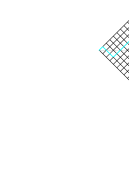
Figure 1: The security price modelled as a walk along a binary tree: it starts at zero and finishes at value $r$ after $n$ steps.

During the $n$-step long random walk process, the price would make $n_{\uparrow}$ steps up and $n_{\downarrow}$ steps down. If the final price is $r$, the following equation should be satisfied:

$$n_{\uparrow}-n_{\downarrow}=r\,.$$ (1)

The total number of steps is $n$, giving the second equaiton

$$n_{\uparrow}+n_{\downarrow}=n\,.$$ (2)

From (1) and (2) it is easy to obtain that $n_{\uparrow}=(n+r)/2$.

The random walk along a binary tree could be constructed as a random choice of up or down moves on every step (equivalent to coin tosses). To reach final value $r$, the price has to make $n_{\uparrow}$ up moves from possible $n$ (fixed amount of ”heads” out of $n$ coin tosses in the fair coin flip analogy). This number is described by the binomial coefficient

$$C_{n}^{n_{\uparrow}}=\frac{n!}{n_{\uparrow}!(n-n_{\uparrow})!}\,.$$

The total number of possible steps on the binary tree is $2^{n}$. Therefore, the probability of the price having the final value $r$ making $n$ random steps (as shown on Fig.1) is

$$P_{n}(r)=\frac{1}{2^{n}}C_{n}^{n_{\uparrow}}=\frac{1}{2^{n}}C_{n}^{\frac{n+r}{2}}\,.$$ (3)

This formula is valid for positive and negative $r$ ($r$ is negative when the price finishes below the starting level). To evaluate the price of limit executions, the probability of the price to have value $r$ after touching (or penetrating) level $k$ is required. The blue line on the left diagram on Fig.2 illustrates the price touching limit level $k$ and finishing at value $r$, the right diagram shows the price penetrating level $k$.

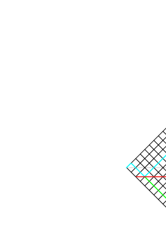
Figure 2: Price could either touch (left diagram) or penetrate (right diagram) the limit level $k$. The blue lines show direct trajectories, the green lines show reflected trajectories which all have the same probabilities of realization.

This probability could be calculated using the technique called reflection which is based on the fact that the probabilities of direct and reflected paths are the same (Feller (1959)). When the price reaches level $k$, it has a choice to move up or down with the same probability. The probability of the real blue path and the probability of reflected path shown by the green line on Fig. 2 are equivalent. The green trajectory finishes at point $2k+r$. Using formula (3), the probability of a price trajectory to touch level $k$ and then finish at a level $r$ is

$$P_{n}(r|k)=P_{n}(2k+r)=\frac{1}{2^{n}}C_{n}^{\frac{n+2k+r}{2}}\,.$$ (4)

To calculate the probability of the price to have the final value $r$ without reaching level $k$, one has to count all the trajectories which finish at $r$ and subtract the number of trajectories which finish in $r$ but touched or crossed limit level $k$. In terms of probabilities, the final result can be obtained using subtraction (4) from (3):

$$P_{n}(r|\overline{k})=P_{n}(r)-P_{n}(r|k)=\frac{1}{2^{n}}\left(C_{n}^{\frac{n+r}{2}}-C_{n}^{\frac{n+2k+r}{2}}\right)\,.$$ (5)

The same formula will be valid for cases when $r$ is negative. If $r$ is a big positive number, there will be cases when no trajectories which end at $r$ could possibly touch or cross level $k$. Fig. 3 illustrates the limit case when the touching is still possible. The maximum amount of down moves in this case is $n_{\downarrow}=k$: the price starts moving down immediately after the start of the trajectory and then bounces. The number of positive steps then is $n_{\uparrow}=n-n_{\downarrow}=n-k$. The price ends at this critical value $r^{*}$, meaning $n_{\uparrow}-n_{\downarrow}=r^{*}$ and $r^{*}=n-2k$. For all $r$ larger than this critical value, the probability to reach this level (without touching $k$) is simply the probability to reach level $r$

$$P_{n}(r|\overline{k})=P_{n}(r)=\frac{1}{2^{n}}C_{n}^{\frac{n+r}{2}}{\quad\rm if\quad}r>n-2k\,.$$ (6)

The probabilities, which were described above, are visualised on Fig. 4: few limit orders with different limit prices are represented by histograms. Sharp peaks on histograms correspond to the position of the limit order. The $k=1$ case is when the limit order is one tick away from the opposite side. According to the chart, almost 70% of all orders in this case will be executed passively. The probabilities of not touching the limit level $P_{n}(r|\overline{k})$ are smaller and behave similarly to the distribution of the price of the underlying instrument (dashed line).

Figure 3: Critical value for $r$. For all $r>r^{*}$ reaching the touch level is not possible.

Figure 4: The distribution of the limit order execution prices for the binary tree with $n=10$.

3 The cost of a static limit order execution

For practical calculations it is useful to shift the starting price to be zero at the beginning of the random walk. Then, positive purchasing price would result in a penalty and negative purchasing price would result in a profit.

Each time the price does not reach a passive level $k$ during the slice time, the trader will need to go aggressive. The aggressive price is going to be $r$, since the price ends up on level $r$. The total penalty for not touching or crossing passive level will be a sum of all penalties over all possible outcomes $r$. The final state cannot be smaller than (or equal to) $-k$ and cannot be larger than the number of steps $n$.

Using (4) and (6), the average cost of execution when the limit level was not reached will be equal to

$$\Delta(\overline{k})=\frac{1}{2^{n}}\left\{\sum_{r=-k+1}^{n-2k}r\left(C_{n}^{\frac{n+r}{2}}-C_{n}^{\frac{n+2k+r}{2}}\right)+\sum_{r=n-2k+1}^{n}rC_{n}^{\frac{n+r}{2}}\right\}\,,$$

or, after regrouping,

$$\Delta(\overline{k})=\frac{1}{2^{n}}\left\{\sum_{r=-k+1}^{n}rC_{n}^{\frac{n+r}{2}}-\sum_{r=-k+1}^{n-2k}rC_{n}^{\frac{n+2k+r}{2}}\right\}\,.$$ (7)

Every time the price touches (or penetrates) the limit order price, the order execution price is $-k$. There are two different possibilities of this situation:

1. The price finishes on level $-k$ or below this level. In this case all the trajectories result in limit executions and the probability of this case can be calculated using (3). The average price of the execution is $-k\times\frac{1}{2^{n}}C_{n}^{\frac{n+r}{2}}$.

2. The price touches or penetrates level $-k$, but ends up above level $-k$. The probability of this situation is calculated using formula (4) and the average price of this type of executions is $-k\times\frac{1}{2^{n}}C_{n}^{\frac{n+2k+r}{2}}$.

The summation over all the possible outcomes of the price action gives the following result:

$$\Delta(k)=\frac{-k}{2^{n}}\left\{\sum_{r=-n}^{-k}C_{n}^{\frac{n+r}{2}}+\sum_{r=-k+1}^{n-2k}C_{n}^{\frac{n+2k+r}{2}}\right\}\,.$$ (8)

The total cost of a limit execution consists of the profit from the situations when the limit price was hit, minus the cost of all the aggressive orders (trajectories without a touch of the limit level). Since the price is counted from zero level, the total execution cost is equal to the price with a minus sign: limit executions give negative price, which means profit. Changing the sign will create a situation where positive values mean a profit:

$$\Delta_{k}=-(\Delta(\overline{k}))+\Delta(k)),$$ (9)

where $\Delta(\overline{k})$ and $\Delta(k)$ are given by (7) and (8).

Using mathematical induction it is possible to prove that $\Delta_{k}=0$, in other words, that the benefit from passive execution is exactly the same as the loss from situations when the limit order was not touched.

By using variables substitution $r\rightarrow r-2k$ in the expressions (7) and (8), the difference of profits for level $k$ and the next level $k+1$ could be written as the following:

$$\Delta_{k+1}-\Delta_{k}=\frac{1}{2^{n}}{\sum_{r=k+1}^{n}C_{n}^{\frac{n+r}{2}}-\sum_{r=-n}^{-k-1}C_{n}^{\frac{n+r}{2}}}\,.$$ (10)

This expression is equal to zero since $C_{n}^{\frac{n+r}{2}}=C_{n}^{\frac{n-r}{2}}$. Therefore for all $k$

$$\Delta_{k+1}=\Delta_{k}\,.$$ (11)

The situation when $k=0$ corresponds to the scenario where the order is placed at the immediate aggressive price for which we know that $\Delta_{k=0}=0$. Consequently, $\Delta_{k}=0$ for all $k$ .

That proves the fact that a passive execution of the slice has no optimal level: all levels always results in a zero gain. This is equivalent to the immediate aggressive execution at the beginning of the slice. This result explains observations of the performance of the Piccolo trading algorithm (Jeria, Schouwenaars, Sofianos [2009]).

4 The risk of the limit order execution

The standard way is to consider the standard deviation $\sigma_{X}^{2}$ of trade outcomes $\delta(r,k)$ as a risk measure of the execution. It should be noted, that $\delta(r,k)$ are not normally distributed for the simple passive strategy.

In the previous section we proved that the average outcome over all possible final values $r$, $\Delta(k)=\sum_{r}{\delta(r,k)P_{n}(r)}=0$ for all $n$. The variance of the execution results has a simple form

$$\sigma_{X}^{2}=\sum_{r}(\delta(r,k)-\Delta_{k})^{2}P_{n}(r)=\sum_{r}\delta(r,k)^{2}P_{n}(r),$$ (12)

where the result depends on the length of the binary tree $n$ and the distance to the limit order $k$. Similarly to the situation with the average cost of execution, the probability of an outcome splits into two components (when the limit order was touched and when the limit level was not reached) $P_{n}(r)=P_{n}(r|k)+P_{n}(r|\overline{k})$. If the limit order was not hit, then the outcome of the price run will be equal to the final price $r$. In analogy with the formula (7),

$$\sigma_{X}^{2}(\overline{k})=\sum_{r}r^{2}P_{n}(r|\overline{k})=\frac{1}{2^{n}}\left\{\sum_{r=-k+1}^{n}r^{2}C_{n}^{\frac{n+r}{2}}-\sum_{r=-k+1}^{n-2k}r^{2}C_{n}^{\frac{n+2k+r}{2}}\right\}\,.$$ (13)

If the the order was executed passively, then, using the same probabilities as in (8),

$$\sigma_{X}^{2}(k)=\sum_{r}(-k)^{2}P_{n}(r|{k})=\frac{k^{2}}{2^{n}}\left\{\sum_{r=-n}^{-k}C_{n}^{\frac{n+r}{2}}+\sum_{r=-k+1}^{n-2k}C_{n}^{\frac{n+2k+r}{2}}\right\}\,.$$ (14)

Comparing this formula and formula (8) for the average execution price when the limit level is hit, it is easy to notice that $\sigma^{2}(k)=-k\Delta(k)$. Using proven relation $\Delta(k)+\Delta(\overline{k})=$0, $\sigma^{2}(k)=-k\Delta(\overline{k})$, the expression (14) could be rewritten via sums present in (13):

$$\sigma_{X}^{2}=\sigma_{X}^{2}(\overline{k})+\sigma_{X}^{2}(k)=\frac{1}{2^{n}}\left\{\sum_{r=-k+1}^{n}(r^{2}+kr)C_{n}^{\frac{n+r}{2}}-\sum_{r=-k+1}^{n-2k}(r^{2}+kr)C_{n}^{\frac{n+2k+r}{2}}\right\}\,.$$ (15)

This expression is exact and is valid for even and odd combinations of parameters $n$ and $k$. After substitution $r^{\prime}\rightarrow r+2k$ in the second term of (15) and simple, but laborious transformations, the variance could be rewritten in the form which reveals its explicit dependency on the limit level $k$:

$$\sigma_{X}^{2}=\frac{1}{2^{n}}\left\{4k\sum_{r=k+1}^{n}rC_{n}^{\frac{n+r}{2}}-2k^{2}\sum_{r=k+1}^{n}C_{n}^{\frac{n+r}{2}}+\sum_{r=-k+1}^{k}r^{2}C_{n}^{\frac{n+r}{2}}\right\},$$ (16)

or, using the definition (3) of probabilities $P_{n}(r)$,

$$\sigma_{X}^{2}=4k\sum_{r=k+1}^{n}rP_{n}(r)-2k^{2}\sum_{r=k+1}^{n}P_{n}(r)+\sum_{r=-k+1}^{k}r^{2}P_{n}(r).$$ (17)

The sum in (17) is performed over all possible values $r$: if the length of the binary tree is an even number, then the final price position $r$ could be only an even number (see Fig.5(a)). If $n$ is an odd number, then possible trajectories ending could only be odd numbers. The level of passive order $k$ is independent and could be any number in the range $[0,n]$.

(a) Probabilities $P_{n}(r)$ for even $n$. The trajectory can finish only in values 0, 2, 4, $\dots$

(b) Halved probabilities $P_{n}(r)$ which are distributed at every point and corresponding normal distribution $N(0,\sqrt{n})$.

Figure 5: Fitting probabilities $P_{n}(r)$ with normal distribution for binary tree.

The first term in the expression (17) provides the main contribution for small values of $k$ and it is linear by this parameter. The second term is smaller and corresponds to the second order of level $k$. It will be shown that the third term corresponds to the cube of level $k$.

5 Analytical approximation for the variance

The summation in (17) which is performed over possible $r$ could be approximated by a summation over all values $r$ with halved probability (see Fig.5(b)). If the tree is large, then the sums with probabilities could be further substituted by the integral over normal distribution $N(0,\sqrt{n})$. In the limit of a large binary tree ($n\rightarrow\infty$) and small values of limit level ($k\rightarrow 0$) the sums could be simplified as the following:

$$\sum_{r=k+1}^{n}rP_{n}(r) \rightarrow \frac{1}{\sqrt{2\pi n}}\int_{k}^{\infty}re^{-\frac{r^{2}}{2n}}dr=\sqrt{\frac{n}{2\pi}}+O\left(\frac{k^{2}}{n}\right),$$

$$\sum_{r=k+1}^{n}P_{n}(r) \rightarrow \frac{1}{\sqrt{2\pi n}}\int_{k}^{\infty}e^{-\frac{r^{2}}{2n}}dr=\frac{1}{2}+O\left(\frac{k}{\sqrt{n}}\right),$$

$$\sum_{r=-k+1}^{k}r^{2}P_{n}(r) \rightarrow \frac{1}{\sqrt{2\pi n}}\int_{-k}^{k}r^{2}e^{-\frac{r^{2}}{2n}}dr=k^{2}\times O\left(\frac{k}{\sqrt{n}}\right).$$

Substituting the values of approximated integrals into expression (17) and terms up to second order over $k$, the approximate formula for standard deviation of the limit order at level $k$ is

$$\sigma_{X}^{2}\approx 4k\sqrt{\frac{n}{2\pi}}-k^{2}\,.$$ (18)

This approximation should be capped with the maximum possible value $n$, which corresponds to the case where level $k\geq n$. Then the limit level is never reached and the variance of the limit order is equal to the variance of the underlying price $\sigma^{2}=n$. Adding this limitation to the approximation (18) will make it work in the whole range of values $k$ as it is shown on Fig.6.

Figure 6: An approximate (18) and exact (17) variances for different limit order levels. They start from zero when the order is executed aggressively at the beginning of the slice and reach maximum value 23 for the selected binary tree size $n=23$. The approximate value is capped by the maximum possible value 23.

The first term in (18), which is linear over limit level $k$, is providing the main contribution. Therefore, the variance of the limit order results $\sigma_{X}^{2}\propto k$ for levels close to the touch, which are the most important during algo trading. Additionally, in real systems a random walk of length $n$ will last the order time $T$. This time describes the dynamic of the system and we will call it a sample time. The standard deviation of the price during the order time is going to be

$$\sigma(T)=\sqrt{n}.$$ (19)

Using this relationship, one can link the standard deviation of the execution $\sigma_{X}(T)$ during the order time $T$ with the standard deviation of price via

$$\sigma_{X}(T)\approx\sqrt{\frac{4k\sigma(T)}{\sqrt{2\pi}}},$$ (20)

where the distance of the limit order to opposite side of the market $k$ is measured in absolute price units.

From another point of view, the size of the system $n$ in real systems is proportional to the time of the order $T$ and formula (18) shows that even putting the limit order one tick away from touch creates a risk which can be expressed via deviation of results as $\sigma(k=1)\propto T^{\frac{1}{4}}$. That fact that even touch orders could possibly have large standard deviation advocates for using dynamic order placing (pegging and adaptive strategies).

6 Probability of a passive fill

The average price of passive executions $\Delta(k)$ calculated in (8) is the product of the price of limit order ($-k$) multiplied by probability of the passive fill $P(k)$. Therefore

$$P(k)=\frac{1}{2^{n}}\left\{\sum_{r=-n}^{-k}C_{n}^{\frac{n+r}{2}}+\sum_{r=-k+1}^{n-2k}C_{n}^{\frac{n+2k+r}{2}}\right\}$$ (21)

Both terms in this expressions are almost identical. Mathematically this can be shown by substituting $r^{\prime}\rightarrow-r$ in the first term and $r^{\prime}\rightarrow r+2k$ in the second term:

$$P(k)=\frac{1}{2^{n}}\left\{\sum_{r=k}^{n}C_{n}^{\frac{n+r}{2}}+\sum_{r=k+1}^{n}C_{n}^{\frac{n+r}{2}}\right\}$$ (22)

The difference between first and the second term in (22) is insignificant. It is equal to zero exactly when $n$ and $k$ have different parity (for example, $n$ is even and $k$ is odd). That could be seen from Fig.3: $r$ cannot be equal to $-k$ with the first available value $r=-k+1$ and $\sum_{r=k}=\sum_{r=k+1}$. In practical calculations, since parameter $n$ is large, we can always select $n$ slightly larger to change its parity. Therefore,

$$P(k)=\frac{2}{2^{n}}\left\{\sum_{r=k+1}^{n}C_{n}^{\frac{n+r}{2}}\right\}=2\sum_{r=k+1}^{n}P_{n}(r),$$ (23)

where $P_{n}(r)$ is the probability to reach point $r$ at the end of the random walk. Converting this sum into an integral, using the procedure described in the previous section (but without the transition $k\rightarrow 0$),

$$P(k,n)=2\sum_{r=k+1}^{n}P_{n}(r)\rightarrow\frac{2}{\sqrt{2\pi n}}\int_{k}^{\infty}e^{-\frac{r^{2}}{2n}}dr=1-{\rm erf}\left(\frac{k}{\sqrt{2n}}\right),$$ (24)

or, using the definition of the standard deviation of the price (19) during the order time $T$ ,

$$P(k,T)=1-{\rm erf}\left(\frac{k}{\sigma(T)\sqrt{2}}\right),$$ (25)

This result can be used to calculate probability at any time. For an arbitrary time $t=\tau T$, the new length $n^{\prime}$ of the binary tree will be extended/shortened by parameter $\tau$ and

$$\sqrt{n^{\prime}}=\sqrt{\tau n}=\sigma(T)\sqrt{\tau}$$ (26)

Substituting this into expression for probability of a passive fill (24), will result in

$$P(k,t=\tau T)=1-{\rm erf}\left(\frac{k}{\sigma(T)\sqrt{2\tau}}\right),$$ (27)

where $\sigma(T)$ is the standard deviation of the price during a sample time $T$.

One can consider important cases of the result (27)

1. $$P(k,t\rightarrow\infty)=1.$$ (28)

   If time of the execution goes to infinity, the price will always hit the limit level. This corresponds to the well known fact that the random walk particle eventually returns to the origin. This principle, applied to algo trading will read any finite limit level in random walk model will be executed passively if the time of the order is infinite. Unfortunately, this will not happen in practice because the time of the order is always limited.

2. $$P(k=\sigma(T),t=T)=1-{\rm erf}\left(\frac{1}{\sqrt{2}}\right)\approx 32\%,$$ (29)

   If the limit order is on the distance of a standard deviation of the price measured for a sample time $T$, then the probability of a passive execution during this time is approximately equal to 32%.

3. $$P(k=\sigma(T),t=2T)=1-{\rm erf}\left(\frac{1}{2}\right)\approx 48\%,$$ (30)

   If the limit order is on the distance of a standard deviation of the price measured for a sample time $T$, then the probability of a passive execution during the double of this time is approximately equal to 48% (roughly half of limit orders will have a passive fill).

7 Conclusions

In this paper we provided an analytical solution to describe the executed price distribution of a strategy where a limit order is placed $k$ ticks away from the best opposite market price and eventually amended at the market price after an elapsed time $T$ if it was not passively filled in between. The analytical solution assumes the price of the underlying instrument follows a random walk process (binomial tree).

The analytical solution shows that the average executed price is always equal to the aggressive market price at the time the strategy is initiated, regardless of the value of $k$. It also shows the variance of the executed prices increases with the distance $k$, as well as with the duration $T$. That corresponds to growing risk of the execution.

Consequently, the best price point for this strategy is the market aggressive price at inception. Working a limit price $k$ ticks away from the initial aggressive price only increases the dispersion of the results without adding any improvements to the average executed price. This conclusion is true for very liquid active markets when the price volatility is much larger than the tick size and the spread size: for illiquid instruments the effect of the queue positioning becomes as important as price fluctuations . This effect introduces additional complexity and is out of the scope of this study.

Therefore, a successful impact avoiding strategy should be complemented with a second layer of market data analysis which proactively decides the best timing to aggress the market (order book imbalance, trades acceleration, etc.). This layer should provide an improved average executed price while trying to minimize the increased variance of the results.

References

- Johnson (2010) \bibinfoauthorB. Johnson, \bibinfotitle Algorithmic Trading & DMA: An Introduction to Direct Access Trading Strategies, \bibinfopublisher4 Myeloma Press, \bibinfoaddressLondon, UK, \bibinfopagespp.118–132, \bibinfoyear2010.
- Markov (2012) \bibinfoauthorV. Markov, \bibinfotitleOn the design of sell-side limit and market order tactics, \bibinfojournalJournal of Trading \bibinfovolume7 \bibinfonumber3 (\bibinfoyear2012), \bibinfopages29–39.