Fault-tolerant bosonic quantum error correction with the surface-GKP code

Abstract

Bosonic quantum error correction is a viable option for realizing error-corrected quantum information processing in continuous-variable bosonic systems. Various single-mode bosonic quantum error-correcting codes such as cat, binomial, and GKP codes have been implemented experimentally in circuit QED and trapped ion systems. Moreover, there have been many theoretical proposals to scale up such single-mode bosonic codes to realize large-scale fault-tolerant quantum computation. Here, we consider the concatenation of the single-mode GKP code with the surface code, namely, the surface-GKP code. In particular, we thoroughly investigate the performance of the surface-GKP code by assuming realistic GKP states with a finite squeezing and noisy circuit elements due to photon losses. By using a minimum-weight perfect matching decoding algorithm on a 3D space-time graph, we show that fault-tolerant quantum error correction is possible with the surface-GKP code if the squeezing of the GKP states is higher than $11.2$dB in the case where the GKP states are the only noisy elements. We also show that the squeezing threshold changes to $18.6$dB when both the GKP states and circuit elements are comparably noisy. At this threshold, each circuit component fails with probability $0.69\%$. Finally, if the GKP states are noiseless, fault-tolerant quantum error correction with the surface-GKP code is possible if each circuit element fails with probability less than $0.81\%$. We stress that our decoding scheme uses the additional information from GKP-stabilizer measurements and we provide a simple method to compute renormalized edge weights of the matching graphs. Furthermore, our noise model is general as it includes full circuit-level noise.

I Introduction

Continuous-variable systems or bosonic modes are ubiquitous in many quantum computing platforms and there have been various proposals for realizing quantum computation in continuous-variable systems Lloyd and Braunstein (1999); Jeong and Kim (2002); Ralph et al. (2003); Lund et al. (2008). Notably, bosonic quantum error correction Albert et al. (2018) has recently risen as a hardware-efficient route to implement quantum error correction (QEC) by taking advantage of the infinite-dimensionality of a bosonic Hilbert space. Various bosonic quantum error-correcting codes include Schrödinger’s cat Cochrane et al. (1999), binomial Michael et al. (2016), and Gottesman-Kitaev-Preskill (GKP) Gottesman et al. (2001) codes. All these codes encode a logical qubit in a physical bosonic oscillator mode and have been realized experimentally in circuit QED Leghtas et al. (2015); Ofek et al. (2016); Touzard et al. (2018); Hu et al. (2019); Campagne-Ibarcq et al. (2019); Grimm et al. (2019) and trapped ion Flühmann et al. (2018, 2019); Flühmann and Home (2019) systems in the past few years.

While bosonic QEC with a single bosonic mode (and a single ancilla qubit) can suppress relevant errors such as photon losses or phase space shift errors in a hardware-efficient way, it should also be noted that logical error rates cannot be suppressed to an arbitrarily small value with this minimal architecture. For example, the experimentally realized four-component cat code and the binomial code cannot correct two (or more) photon loss events. Similarly, the GKP code cannot correct phase space shift errors of a size larger than a critical value. Therefore, to further suppress the residual errors, these bosonic codes should, for example, be concatenated with some other error-correcting code families such as the surface code Bravyi and Kitaev (1998); Dennis et al. (2002); Fowler et al. (2012).

Recently, there have been proposals for scaling up the cat codes by concatenating them with a repetition code Guillaud and Mirrahimi (2019) or a surface code Puri et al. (2019) which are tailored to biased noise models Tuckett et al. (2018, 2018, 2019). These schemes take advantage of the fact that the cat code can suppress bosonic dephasing (stochastic random rotation) errors exponentially in the size of the cat code, thereby yielding a qubit with a biased noise predominated either by bit-flip or phase-flip errors. These studies have shown that the gates on the cat code needed for the concatenation can be implemented in a noise-bias-preserving way. On the other hand, the full concatenated error correction schemes have not been thoroughly studied in these works.

Meanwhile, there have also been studies on scaling up the GKP code by concatenating it with a repetition code Fukui et al. (2017), the $[[4,2,2]]$ code Fukui et al. (2017, 2018a), and the surface code Wang (2017); Fukui et al. (2018b); Vuillot et al. (2019), or by using cluster states and measurement-based quantum computation Menicucci (2014); Fukui et al. (2018b); Fukui (2019). One of the recurring themes in these previous works is that the continuous error information gathered during the GKP code error correction protocol can boost the performance of the next layer of the concatenated error correction. For example, while the surface code by itself has the code capacity threshold $\sim\!\!11\%$ Dennis et al. (2002), the threshold can be increased to $\sim\!\!14\%$ if the additional error information from GKP-stabilizer measurements is incorporated in the surface code error correction protocol Wang (2017); Fukui et al. (2018b); Vuillot et al. (2019). However, note that the code capacity thresholds are obtained by assuming that only qubits can fail, i.e., gates, state preparations, and measurements are assumed perfect. Hence, the above code capacity threshold for the concatenated GKP code is evaluated by assuming noiseless GKP and surface code stabilizer measurements, or equivalently, by assuming that ideal GKP states (with an infinitely large squeezing) are used for the stabilizer measurements.

If the error syndrome is extracted using realistic GKP states with a finite squeezing, the error correction protocols would become faulty. Nevertheless, in the framework of measurement-based quantum computation Raussendorf et al. (2003), it has been shown that fault-tolerant quantum error correction with finitely-squeezed GKP states is possible if the strength of the squeezing is above a certain threshold. Specifically, the recent works Fukui et al. (2018b); Fukui (2019) have demonstrated that the threshold value can be brought down from $\sim\!\!20$dB Menicucci (2014) to less than $10$dB by using post-selection.

In the framework of gate-based quantum computation, several fault-tolerance thresholds have been computed for the GKP code concatenated with the toric code, namely the toric-GKP code, by assuming a phenomenological noise model Vuillot et al. (2019); Wang (2017). In these previous works, however, shift errors were manually added instead of being derived from an underlying noise model for realistic GKP states and the noisy circuits used for stabilizer measurements.

In our work, we thoroughly investigate the full error correction protocol for the GKP code concatenated with the surface code, namely, the surface-GKP code. We choose the surface code for the next level of encoding because it can be implemented in a geometrically local way in a planar architecture. In particular, we consider a detailed circuit-level noise model and assume that every GKP state supplied to the error correction chain is finitely squeezed, and also that every circuit element can be noisy due to photon losses and heating. Unlike previous works such as in Vuillot et al. (2019); Wang (2017) (where noise propagation was not considered), we comprehensively take into account the propagation of such imperfections throughout the entire circuit and simulate the full surface code error correction protocol assuming this general circuit-level noise model. Finally, by using a simple decoding algorithm based on a minimum-weight perfect matching (MWPM) Edmonds (1965a, b) algorithm applied to 3D space-time graphs, we establish that fault-tolerant quantum error correction is possible if the squeezing of the GKP states is higher than $11.2$dB when the GKP states are the only noisy components, or than $18.6$dB when both the GKP states and circuit elements are comparably noisy. In the latter case, each circuit element that implements the surface-GKP code fails with probability $0.69\%$. In the case where GKP states are noiseless, we find that fault-tolerant quantum error correction with the surface-GKP code is possible if each circuit element fails with probability less than $0.81\%$. In general, it has been shown that using edge weights in the matching graphs which are computed from the most likely error configurations can significantly improve the performance of a topological code Wang et al. (2011); Chamberland et al. (2019). Our decoding algorithm provides a simple way to compute renormalized edge weights of the 3D matching graphs, tailored to our general circuit-level noise model, based on information obtained from GKP-stabilizer measurements.

Our paper is organized as follows: In Section II, we introduce the surface-GKP code and describe the noise model that we assume for the fault-tolerance study. In Section III, we summarize the main results and establish fault-tolerance thresholds. A detailed description of our analysis is given in Appendix B. In Section IV, we compare our results with the previous ones and conclude the paper with an outlook.

II The surface-GKP code

In this section, we introduce the surface-GKP code, i.e., GKP qubits concatenated with the surface code. The GKP qubits are constructed by using the standard square-lattice GKP code that encodes a single qubit into an oscillator mode Gottesman et al. (2001), which is reviewed in Section II.1. For the next layer of the encoding, we use the family of rotated surface codes that requires $d^{2}$ data qubits and $d^{2}-1$ syndrome qubits where $d\in\{2n+1:n\in\mathbb{N}\}$ is the distance of the code Bombin and Martin-Delgado (2007); Tomita and Svore (2014). In Section II.2, we construct the surface-GKP code and discuss its implementation. In Section II.3, we introduce the noise model that we use to simulate the full noisy error correction protocol for the surface-GKP code. Readers who are familiar with the GKP code and the surface code may skip Sections II.1 and II.2 and are referred to Section II.3.

II.1 GKP qubit

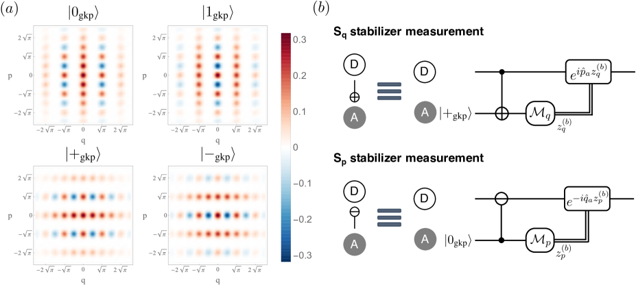
Figure 1: (a) Computational basis states ($|0_{\textrm{gkp}}\rangle$, $|1_{\textrm{gkp}}\rangle$) and complementary basis states ($|+_{\textrm{gkp}}\rangle$, $|-_{\textrm{gkp}}\rangle$) of an approximate GKP qubit with an average photon number $\bar{n}=5$. (b) Circuits for measuring the $\hat{S}_{q}$ and $\hat{S}_{p}$ stabilizers. $\mathcal{M}_{q}$ and $\mathcal{M}_{p}$ represent the homodyne measurement of the position and momentum operators, respectively. Also, the controlled-$\oplus$ symbol represents the SUM gate and similarly the controlled-$\ominus$ symbol represents the inverse-SUM gate (see Eq. 6). Note that the size of the correction shifts $\exp[i\hat{p}_{a}z_{q}^{(b)}]$ and $\exp[-i\hat{q}_{a}z_{p}^{(b)}]$ in the $\hat{S}_{q}$ and $\hat{S}_{p}$ stabilizer measurements are determined by the homodyne measurement outcomes $z_{q}^{(b)}$ and $z_{p}^{(b)}$.

Let $\hat{q}=(\hat{a}^{\dagger}+\hat{a})/\sqrt{2}$ and $\hat{p}=i(\hat{a}^{\dagger}-\hat{a})/\sqrt{2}$ be the position and momentum operators of a bosonic mode, where $\hat{a}$ and $\hat{a}^{\dagger}$ are annihilation and creation operators satisfying $[\hat{a},\hat{a}^{\dagger}]=1$. We define the GKP qubit as the $2$-dimensional subspace of a bosonic Hilbert space that is stabilized by the two stabilizers

$$\hat{S}_{q}\equiv\exp[i2\sqrt{\pi}\hat{q}],\quad\hat{S}_{p}\equiv\exp[-i2\sqrt{\pi}\hat{p}].$$ (1)

Measuring these two commuting stabilizers is equivalent to measuring the position and momentum operators $\hat{q}$ and $\hat{p}$ modulo $\sqrt{\pi}$. Therefore, any phase space shift error $\exp[i(\xi_{p}\hat{q}-\xi_{q}\hat{p})]$ acting on the ideal GKP qubit can be detected and corrected as long as $|\xi_{q}|,|\xi_{p}|<\sqrt{\pi}/2$.

Explicitly, the computational basis states of the ideal GKP qubit are given by

$$|0_{\textrm{gkp}}\rangle =\sum_{n\in\mathbb{Z}}|\hat{q}=2n\sqrt{\pi}\rangle,$$

$$|1_{\textrm{gkp}}\rangle =\sum_{n\in\mathbb{Z}}|\hat{q}=(2n+1)\sqrt{\pi}\rangle.$$ (2)

Also, the complementary basis states $|\pm_{\textrm{gkp}}\rangle\equiv\frac{1}{\sqrt{2}}(|0_{\textrm{gkp}}\rangle\pm|1_{\textrm{gkp}}\rangle)$ are given by

$$|+_{\textrm{gkp}}\rangle =\sum_{n\in\mathbb{Z}}|\hat{p}=2n\sqrt{\pi}\rangle,$$

$$|-_{\textrm{gkp}}\rangle =\sum_{n\in\mathbb{Z}}|\hat{p}=(2n+1)\sqrt{\pi}\rangle.$$ (3)

Clearly, all these basis states have $\hat{q}=\hat{p}=0$ modulo $\sqrt{\pi}$ and thus are stabilized by $\hat{S}_{q}$ and $\hat{S}_{p}$.

The ideal GKP qubit states consist of infinitely many infinitely-squeezed states and thus are unrealistic. Realistic GKP qubit states can be obtained by applying a Gaussian envelope operator $\exp[-\Delta\hat{n}]$ to the ideal GKP states, i.e., $|\psi^{\Delta}_{\textrm{gkp}}\rangle\propto\exp[-\Delta\hat{n}]|\psi_{\textrm{gkp}}\rangle$ and have a finite average photon number or finite squeezing. Here, $\hat{n}=\hat{a}^{\dagger}\hat{a}$ is the excitation number operator and $\Delta$ characterizes the width of each peak in the Wigner function of a realistic GKP state. In Fig. 1 (a), we plot the Wigner functions of the basis states of an approximate GKP qubit with $\bar{n}=5$. There are many proposals for realizing approximate GKP states in various experimental platforms Gottesman et al. (2001); Travaglione and Milburn (2002); Pirandola et al. (2004, 2006); Vasconcelos et al. (2010); Terhal and Weigand (2016); Motes et al. (2017); Weigand and Terhal (2018); Arrazola et al. (2019); Su et al. (2019); Eaton et al. (2019); Shi et al. (2019); Weigand and Terhal (2019). Notably, approximate GKP states have been realized experimentally in circuit QED Campagne-Ibarcq et al. (2019) and trapped ion systems Flühmann et al. (2018, 2019); Flühmann and Home (2019). In Section II.3, we discuss the adverse effects of the finite photon number in more detail. In this subsection, we instead focus on the properties of an ideal GKP qubit.

Pauli operators of the GKP qubit are given by the square root of the stabilizers, i.e.,

$$\hat{Z}_{\textrm{gkp}} =(\hat{S}_{q})^{\frac{1}{2}}=\exp[i\sqrt{\pi}\hat{q}],$$

$$\hat{X}_{\textrm{gkp}} =(\hat{S}_{p})^{\frac{1}{2}}=\exp[-i\sqrt{\pi}\hat{p}].$$ (4)

Indeed, one can readily check that these Pauli operators act on the computational basis states as desired:

$$\hat{Z}_{\textrm{gkp}}|0_{\textrm{gkp}}\rangle =|0_{\textrm{gkp}}\rangle,\quad \hat{Z}_{\textrm{gkp}}|1_{\textrm{gkp}}\rangle =-|1_{\textrm{gkp}}\rangle,$$

$$\hat{X}_{\textrm{gkp}}|0_{\textrm{gkp}}\rangle =|1_{\textrm{gkp}}\rangle,\quad \hat{X}_{\textrm{gkp}}|1_{\textrm{gkp}}\rangle =|0_{\textrm{gkp}}\rangle.$$ (5)

Clifford operations Gottesman and Chuang (1999) on the GKP qubits can be implemented by using only Gaussian operations. More explicitly, generators of the Clifford group, $\hat{S}_{\textrm{gkp}},\hat{H}_{\textrm{gkp}}$ and $\textrm{CNOT}_{\textrm{gkp}}^{j\rightarrow k}$ are given by

$$\hat{S}_{\textrm{gkp}} =\exp\Big{[}i\frac{\hat{q}^{2}}{2}\Big{]},$$

$$\hat{H}_{\textrm{gkp}} =\exp\Big{[}i\frac{\pi}{2}\hat{a}^{\dagger}\hat{a}\Big{]},$$

$$\textrm{CNOT}_{\textrm{gkp}}^{j\rightarrow k} =\textrm{SUM}_{j\rightarrow k}\equiv\exp[-i\hat{q}_{j}\hat{p}_{k}],$$ (6)

and one can similarly check that

$$\hat{S}_{\textrm{gkp}}|0_{\textrm{gkp}}\rangle =|0_{\textrm{gkp}}\rangle,\quad \hat{S}_{\textrm{gkp}}|1_{\textrm{gkp}}\rangle =i|1_{\textrm{gkp}}\rangle,$$

$$\hat{H}_{\textrm{gkp}}|0_{\textrm{gkp}}\rangle =|+_{\textrm{gkp}}\rangle,\quad \hat{H}_{\textrm{gkp}}|1_{\textrm{gkp}}\rangle =|-_{\textrm{gkp}}\rangle,$$ (7)

and

$$\textrm{CNOT}_{\textrm{gkp}}^{j\rightarrow k}|\mu^{(j)}_{\textrm{gkp}}\rangle|\nu^{(k)}_{\textrm{gkp}}\rangle=|\mu^{(j)}_{\textrm{gkp}}\rangle|(\mu\oplus\nu)^{(k)}_{\textrm{gkp}}\rangle,$$ (8)

for all $\mu,\nu\in\mathbb{Z}_{2}$, where $|\mu^{(j)}_{\textrm{gkp}}\rangle\equiv\sum_{n\in\mathbb{Z}}|\hat{q}_{j}=(2n+\mu)\sqrt{\pi}\rangle$ is the GKP state in the $j^{\textrm{th}}$ mode and $\oplus$ is the addition modulo $2$.

Recall that measuring the stabilizers of the GKP qubit $\hat{S}_{q}$ and $\hat{S}_{p}$ is equivalent to measuring the position and the momentum operators $\hat{q}$ and $\hat{p}$ modulo $\sqrt{\pi}$. These measurements can be respectively performed by preparing an ancilla GKP state $|+_{\textrm{gkp}}\rangle$ or $|0_{\textrm{gkp}}\rangle$, and then applying the $\textrm{SUM}_{D\rightarrow A}$ or $\textrm{SUM}_{A\rightarrow D}^{\dagger}$ gate, and finally measuring the position or the momentum operator of the ancilla mode via a homodyne detection (see Fig. 1 (b)). Here, $D$ refers to the data mode and $A$ refers to the ancilla mode. Note that the only non-Gaussian resources required for the GKP-stabilizer measurements are the ancilla GKP states $|0_{\textrm{gkp}}\rangle$ and $|+_{\textrm{gkp}}\rangle$.

Now, consider the Gaussian random displacement error channel $\mathcal{N}[\sigma]$ defined as

$$\mathcal{N}[\sigma](\hat{\rho})\equiv\int\frac{d^{2}\alpha}{\pi\sigma^{2}}\exp\Big{[}-\frac{|\alpha|^{2}}{\sigma^{2}}\Big{]}\hat{D}(\alpha)\hat{\rho}\hat{D}^{\dagger}(\alpha),$$ (9)

where $\hat{D}(\alpha)\equiv\exp[\alpha\hat{a}^{\dagger}-\alpha^{*}\hat{a}]$ is the displacement operator and $\alpha\in\mathbb{C}$ is the amplitude of the displacement. In the Heisenberg picture, the error channel $\mathcal{N}[\sigma]$ adds shift errors to the position and momentum quadratures, that is, $\hat{q}\rightarrow\hat{q}+\xi_{q}$ and $\hat{p}\rightarrow\hat{p}+\xi_{p}$, where $\xi_{q}$ and $\xi_{p}$ follow a Gaussian random distribution with zero mean and standard deviation $\sigma$: $\xi_{q},\xi_{p}\sim\mathcal{N}(0,\sigma)$. If, for example, the size of the random position shift $\xi_{q}$ is smaller than $\sqrt{\pi}/2$ (i.e., $|\xi_{q}|<\sqrt{\pi}/2$), the shift can be correctly identified by measuring the GKP stabilizer $\hat{S}_{q}$. However, if $\xi_{q}$ lies in the range $|\xi_{q}-\sqrt{\pi}|<\sqrt{\pi}/2$, the shift is incorrectly identified as a smaller shift $\xi_{q}-\sqrt{\pi}$. Then, such a misidentification results in a residual shift $\exp[-i\sqrt{\pi}\hat{p}]=\hat{X}_{\textrm{gkp}}$ and thus causes a Pauli $X$ error on the GKP qubit.

In general, if $\xi_{q}$ (or $\xi_{p}$) lies in the range $|\xi_{q}-n\sqrt{\pi}|<\sqrt{\pi}/2$ (or $|\xi_{p}-n\sqrt{\pi}|<\sqrt{\pi}/2$) for an odd integer $n$, the GKP error correction protocol results in a Pauli $X$ (or $Z$) error on the GKP qubit and this happens with probability $p_{\textrm{err}}(\sigma)$, where $p_{\textrm{err}}(\sigma)$ is defined as

$$p_{\textrm{err}}(\sigma) \equiv\sum_{n\in\mathbb{Z}}\frac{1}{\sqrt{2\pi\sigma^{2}}}\int_{(2n+\frac{1}{2})\sqrt{\pi}}^{(2n+\frac{3}{2})\sqrt{\pi}}d\xi\exp\Big{[}-\frac{\xi^{2}}{2\sigma^{2}}\Big{]}.$$ (10)

Now, consider a specific instance where, for example, the $\hat{S}_{q}$ stabilizer measurement (i.e., the position measurement modulo $\sqrt{\pi}$) informs us that $\xi_{q}$ is given by $\xi_{q}=z+n\sqrt{\pi}$ for some interger $n$ and $|z|<\sqrt{\pi}/2$. Then, since odd $n$ corresponds to a Pauli $X$ error and even $n$ corresponds to the no error case, we can infer that, given the measured value $z$, there is a Pauli $X$ error with probability $p[\sigma](z)$ where $p[\sigma](z)$ is defined as

$$p[\sigma](z) \equiv\frac{\sum_{n\in\mathbb{Z}}\exp[-(z-(2n+1)\sqrt{\pi})^{2}/(2\sigma^{2})]}{\sum_{n\in\mathbb{Z}}\exp[-(z-n\sqrt{\pi})^{2}/(2\sigma^{2})]}.$$ (11)

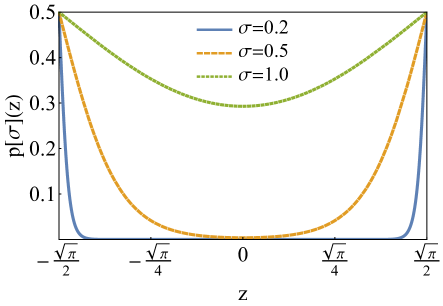
Figure 2: $p[\sigma](z)$ for $\sigma=0.2$, $0.5$, and $1$. $p[\sigma](z)$ is defined in Eq. 11 and represents the conditional probability of having a Pauli $X$ (or $Z$) error, given the measurement outcome $\xi_{q}=z+n\sqrt{\pi}$ (or $\xi_{p}=z+n\sqrt{\pi}$) for some integer $n$.

As shown in Fig. 2, the conditional probability $p[\sigma](z)$ becomes larger as $|z|$ gets closer to the decision boundary $\sqrt{\pi}/2$. Therefore, if the measured shift value modulo $\sqrt{\pi}$ is close to $\pm\sqrt{\pi}/2$, we know that this specific instance of the GKP error correction is less reliable. This way, the GKP error correction protocol not only corrects the small shift errors but also informs us how reliable the correction is. Various ways of incorporating this additional information in the next level of concatenated error correction have been studied in Refs. Fukui et al. (2017, 2018b, 2018a); Fukui (2019); Vuillot et al. (2019). In Appendix B, we explain in detail how the additional information from GKP-stabilizer measurements can be used to compute renormalized edge weights of the matching graphs used in the surface code error correction protocol.

Lastly, although not relevant to the purpose of our work, it has been shown that a H-type GKP-magic state $|H_{\textrm{gkp}}\rangle=\cos(\frac{\pi}{8})|0_{\textrm{gkp}}\rangle+\sin(\frac{\pi}{8})|1_{\textrm{gkp}}\rangle$ can be prepared by performing GKP-stabilizer measurements on a vacuum state and then post-selecting the $\hat{S}_{q}=\hat{S}_{p}=1$ (or $\hat{q}=\hat{p}=0$ modulo $\sqrt{\pi}$) event Terhal and Weigand (2016) (see Ref. Bravyi and Kitaev (2005) for more details on the magic states). Notably, a more recent study Baragiola et al. (2019) has quantitatively showed that any post-measurement state after the GKP-stabilizer measurements (on a vacuum state) is a distillable GKP-magic state and therefore post-selection is not necessary. Since Clifford operations (necessary for magic state distillation) on GKP qubits can be implemented by using only Gaussian operations, the ability to prepare GKP states is the only non-Gaussian resource needed for universal quantum computation using GKP qubits.

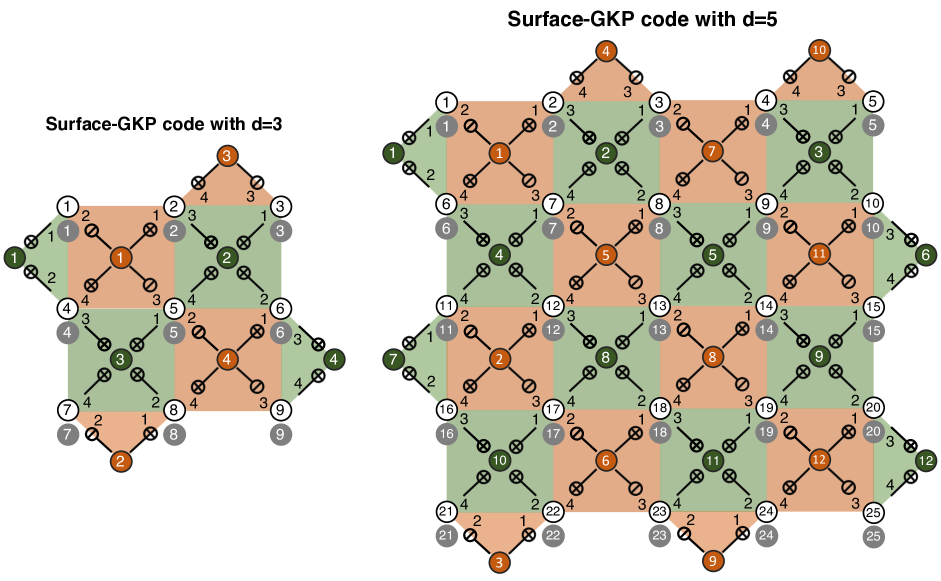
Figure 3: The surface-GKP codes with $d=3$ and $d=5$. White circles represent the data GKP qubits and grey circles represent the ancilla GKP qubits that are used to measure GKP stabilizers of each data GKP qubit. Green and orange circles represent the syndrome GKP qubits that are used to measure the $Z$-type and $X$-type surface code stabilizers of the data GKP qubits, respectively. In general, there are $d^{2}$ data GKP qubits and $(d^{2}-1)/2$ $Z$-type and $X$-type syndrome GKP qubits. See also Fig. 5 for the reason behind our choice of inverse-SUM gates in the $X$-type stabilizer measurements.

II.2 The surface code with GKP qubits

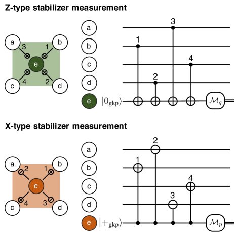
Figure 4: Circuits for surface code stabilizer measurements.

Recall that shift errors of size larger than $\sqrt{\pi}/2$ cannot be corrected by the single-mode GKP code. Here, to correct arbitrarily large shift errors, we consider the concatenation of the GKP code with the surface code Bravyi and Kitaev (1998); Dennis et al. (2002); Fowler et al. (2012), namely, the surface-GKP code. Specifically, we use the family of rotated surface codes Bombin and Martin-Delgado (2007); Tomita and Svore (2014) that only requires $d^{2}$ data qubits and $d^{2}-1$ syndrome qubits to get a distance-$d$ code. Note that the distance-$d$ surface code can correct arbitrary qubit errors of weight less than or equal to $\lfloor\frac{d-1}{2}\rfloor$.

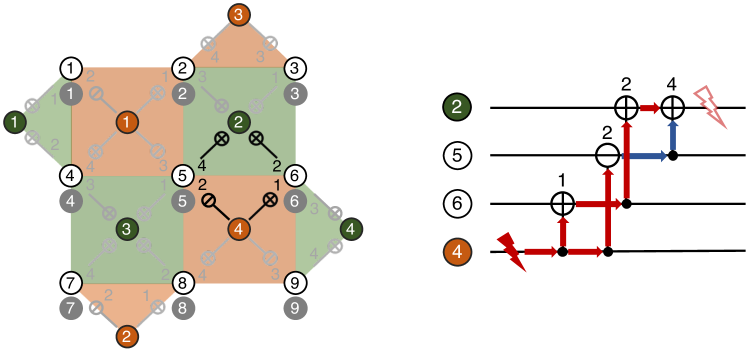
Figure 5: Noise propagation from the X4 qubit to the Z2 qubit during surface code stabilizer measurements. The red lightening symbol represents the initial position of a shift error on the qubit X4. During the propagation of the shift error to the qubit Z2, the sign of the shift error is flipped by the inverse-SUM gate $\textrm{SUM}^{\dagger}_{X4\rightarrow D5}$. This sign flip then results in cancellations of the propagated shift errors on the qubit Z2 (empty lightening symbol).

The layout for the data and ancilla qubits of the surface-GKP code is given in Fig. 3. Each of the $d^{2}$ data qubits (white circles in Fig. 3) corresponds to a GKP qubit as defined in Section II.1. That is, the distance-$d$ surface-GKP code is stabilized by the following $2d^{2}$ GKP stabilizers

$$\hat{S}_{q}^{(k)}\equiv\exp[i2\sqrt{\pi}\hat{q}_{k}],\quad\hat{S}_{p}^{(k)}\equiv\exp[-i2\sqrt{\pi}\hat{p}_{k}],$$ (12)

for $k\in\{1,\cdots,d^{2}\}$. These GKP stabilizers are measured by $d^{2}$ ancilla GKP qubits (grey circles in Fig. 3) using the circuits given in Fig. 1 (b). Moreover, the data GKP qubits are further stabilized by the $d^{2}-1$ surface code stabilizers. For example, in the $d=3$ case, the $8$ surface code stabilizers are explicitly given by

$$\hat{S}_{Z}^{(1)} =\hat{Z}_{\textrm{gkp}}^{(1)}\hat{Z}_{\textrm{gkp}}^{(4)},\quad \hat{S}_{Z}^{(2)} =\hat{Z}_{\textrm{gkp}}^{(2)}\hat{Z}_{\textrm{gkp}}^{(3)}\hat{Z}_{\textrm{gkp}}^{(5)}\hat{Z}_{\textrm{gkp}}^{(6)},$$

$$\hat{S}_{Z}^{(3)} =\hat{Z}_{\textrm{gkp}}^{(4)}\hat{Z}_{\textrm{gkp}}^{(5)}\hat{Z}_{\textrm{gkp}}^{(7)}\hat{Z}_{\textrm{gkp}}^{(8)},\quad \hat{S}_{Z}^{(4)} =\hat{Z}_{\textrm{gkp}}^{(6)}\hat{Z}_{\textrm{gkp}}^{(9)},$$ (13)

and

$$\hat{S}_{X}^{(1)} =(\hat{X}_{\textrm{gkp}}^{(1)})^{\dagger}\hat{X}_{\textrm{gkp}}^{(2)}\hat{X}_{\textrm{gkp}}^{(4)}(\hat{X}_{\textrm{gkp}}^{(5)})^{\dagger},\quad\hat{S}_{X}^{(2)}=(\hat{X}_{\textrm{gkp}}^{(7)})^{\dagger}\hat{X}_{\textrm{gkp}}^{(8)},$$

$$\hat{S}_{X}^{(3)} =\hat{X}_{\textrm{gkp}}^{(2)}(\hat{X}_{\textrm{gkp}}^{(3)})^{\dagger},\quad\hat{S}_{X}^{(4)}=(\hat{X}_{\textrm{gkp}}^{(5)})^{\dagger}\hat{X}_{\textrm{gkp}}^{(6)}\hat{X}_{\textrm{gkp}}^{(8)}(\hat{X}_{\textrm{gkp}}^{(9)})^{\dagger},$$ (14)

where $\hat{Z}_{\textrm{gkp}}^{(k)}\equiv\exp[i\sqrt{\pi}\hat{q}_{k}]$ and $\hat{X}_{\textrm{gkp}}^{(k)}\equiv\exp[-i\sqrt{\pi}\hat{p}_{k}]$ (see Fig. 3).

As shown in Fig. 4, the $Z$-type surface code stabilizers are measured by the $Z$-type GKP syndrome qubits (green circles in Fig. 3) by using the SUM gates $\textrm{SUM}_{a\rightarrow e},\cdots,\textrm{SUM}_{d\rightarrow e}$ and the position homodyne measurement $\mathcal{M}_{q}$. Similarly, the $X$-type surface code stabilizers are measured by the $X$-type GKP syndrome qubits (orange circles in Fig. 3) by using the SUM and the inverse-SUM gates $\textrm{SUM}_{e\rightarrow a}^{\dagger},\textrm{SUM}_{e\rightarrow b},\textrm{SUM}_{e\rightarrow c},\textrm{SUM}_{e\rightarrow d}^{\dagger}$ and the momentum homodyne measurement $\mathcal{M}_{p}$. Note that all the $Z$-type and $X$-type surface code stabilizers can be measured in parallel without conflicting with each other, if the SUM and the inverse-SUM gates are executed in an order that is specified in Figs. 3 and 4.

We remark that in the usual case where the surface code is implemented with bare qubits (such as transmons Koch et al. (2007); Schreier et al. (2008)), it makes no difference to replace, for example, $\hat{S}_{X}^{(1)}=(\hat{X}^{(1)})^{\dagger}\hat{X}^{(2)}\hat{X}^{(4)}(\hat{X}^{(5)})^{\dagger}$ by $\hat{S}_{X}^{(1)}=\hat{X}^{(1)}\hat{X}^{(2)}\hat{X}^{(4)}\hat{X}^{(5)}$ since the Pauli operators are hermitian. Similarly, the action of $(\hat{X}_{\textrm{gkp}}^{(k)})^{\dagger}$ on the GKP qubit subspace is identical to that of $\hat{X}_{\textrm{gkp}}^{(k)}$ and therefore measuring $\hat{S}_{X}^{(1)}=(\hat{X}_{\textrm{gkp}}^{(1)})^{\dagger}\hat{X}_{\textrm{gkp}}^{(2)}\hat{X}_{\textrm{gkp}}^{(4)}(\hat{X}_{\textrm{gkp}}^{(5)})^{\dagger}$ is equivalent to measuring $\hat{S}_{X}^{(1)}=\hat{X}_{\textrm{gkp}}^{(1)}\hat{X}_{\textrm{gkp}}^{(2)}\hat{X}_{\textrm{gkp}}^{(4)}\hat{X}_{\textrm{gkp}}^{(5)}$ in the case of the surface-GKP code if the syndrome measurements are noiseless.

It is important to note, however, that the actions of $(\hat{X}_{\textrm{gkp}}^{(k)})^{\dagger}$ and $\hat{X}_{\textrm{gkp}}^{(k)}$ are not the same outside of the GKP qubit subspace. Therefore, it does make a difference to choose $(\hat{X}_{\textrm{gkp}}^{(k)})^{\dagger}$ instead of $\hat{X}_{\textrm{gkp}}^{(k)}$ in the noisy measurement case, since shift errors propagate differently depending on the choice. For example, we illustrate in Fig. 5 how the initial position shift error in the fourth $X$-type syndrome GKP qubit (X4 qubit) propagates to the second $Z$-type syndrome GKP qubit (Z2 qubit) through the fifth and the sixth data GKP qubits (D5 and D6 qubits). Note that an initial random position shift in the X4 qubit (represented by the red lightning symbol) is propagated to the D6 qubit via the SUM gate $\textrm{SUM}_{X4\rightarrow D6}$ and then to the Z2 qubit via $\textrm{SUM}_{D6\rightarrow Z2}$. Additionally, it is also propagated to the D5 qubit via the inverse-SUM gate $\textrm{SUM}^{\dagger}_{X4\rightarrow D5}$ with its sign flipped and then the flipped shift is further propagated to the Z2 qubit via $\textrm{SUM}_{D5\rightarrow Z2}$. Thus, the propagated shift errors eventually cancel out each other at the Z2 qubit (visualized by the empty lightning symbol) due to the sign flip during the inverse-SUM gate.

Note that if the SUM gate $\textrm{SUM}_{X4\rightarrow D5}$ were used instead of the inverse-SUM gate $\textrm{SUM}^{\dagger}_{X4\rightarrow D5}$, the propagated shift errors would add together and therefore be amplified by a factor of $2$. In this regard, we emphasize that we have carefully chosen the specific pattern of the SUM and the inverse-SUM gates in Fig. 3 to avoid such noise amplifications.

II.3 Noise model

In this section we discuss the noise model that we use to simulate the full error correction protocol with the surface-GKP code. To be more specific, the surface-GKP error correction protocol is implemented by repeatingly measuring the $\hat{S}_{q}$ and $\hat{S}_{p}$ GKP stabilizers for each data GKP qubit by using the circuits in Fig. 1 (b), and then measuring the surface code stabilizers shown in Figs. 3 and 4. Note that the required resources for these measurements are as follows:

• Preparation of the GKP states $|0_{\textrm{gkp}}\rangle$ and $|+_{\textrm{gkp}}\rangle$.

• SUM and inverse-SUM gates.

• Position and momentum homodyne measurements.

• Displacement operations for error correction.

We assume that all these components can be noisy except for the displacement operations since in most experimental platforms, the errors associated with the displacement operations are negligible compared to the other errors. Moreover, note that displacement operations are only needed for error correction. Thus, they need not be implemented physically in practice since they can be kept track of by using a Pauli frame Knill (2005); DiVincenzo and Aliferis (2007); Terhal (2015); Chamberland et al. (2018). Below, we describe the noise model for each component in more detail.

Let us recall that realistic GKP states have a finite average photon number, or finite squeezing. As discussed in Section II.1, a finite-size GKP state can be modeled by applying a Gaussian envelope operator $\exp[-\Delta\hat{n}]$ to an ideal GKP state, i.e., $|\psi_{\textrm{gkp}}^{\Delta}\rangle\propto\exp[-\Delta\hat{n}]|\psi_{\textrm{gkp}}\rangle$. Expanding the envelope operator in terms of displacement operators Cahill and Glauber (1969), we can write

$$|\psi_{\textrm{gkp}}^{\Delta}\rangle \propto\int\frac{d^{2}\alpha}{\pi}\textrm{Tr}\big{[}\exp[-\Delta\hat{n}]\hat{D}^{\dagger}(\alpha)\big{]}\hat{D}(\alpha)|\psi_{\textrm{gkp}}\rangle$$

$$\propto\int d^{2}\alpha\exp\Big{[}-\frac{|\alpha|^{2}}{2\sigma_{\textrm{gkp}}^{2}}\Big{]}\hat{D}(\alpha)|\psi_{\textrm{gkp}}\rangle,$$ (15)

where $\sigma_{\textrm{gkp}}^{2}=(1-e^{-\Delta})/(1+e^{-\Delta})\xrightarrow{\Delta\ll 1}\Delta/2$ (see Eq. 22). That is, an approximate GKP state can be understood as the state that results from applying coherent superpositions of displacement operations with a Gaussian envelope to an ideal GKP state. More details about the approximate GKP codes can be found in Terhal and Weigand (2016); Shi et al. (2019); Pantaleoni et al. (2019); Tzitrin et al. (2019); Matsuura et al. (2019).

To simplify our analysis of the surface-GKP code, we consider noisy GKP states corrupted by an incoherent mixture of displacement operations, instead of the coherent superposition as in Eq. 15. That is, whenever a fresh GKP state $|0_{\textrm{gkp}}\rangle$ or $|+_{\textrm{gkp}}\rangle$ is supplied to the error correction chain, we assume that a noisy GKP state

$$|0_{\textrm{gkp}}\rangle \rightarrow\mathcal{N}[\sigma_{\textrm{gkp}}](|0_{\textrm{gkp}}\rangle\langle 0_{\textrm{gkp}}|),\textrm{ or}$$

$$|+_{\textrm{gkp}}\rangle \rightarrow\mathcal{N}[\sigma_{\textrm{gkp}}](|+_{\textrm{gkp}}\rangle\langle+_{\textrm{gkp}}|)$$ (16)

is supplied where the Gaussian random displacement error $\mathcal{N}[\sigma]$ is defined in Eq. 9. Note that $\mathcal{N}[\sigma]$ models an incoherent mixture of random displacement errors. We remark that the noisy GKP states corrupted by an incoherent displacement error (as in Eq. 16) are noisier than the noisy GKP states corrupted by a coherent displacement error (as in Eq. 15), because the former can be obtained from the latter by applying a technique similar to Pauli twirling Emerson et al. (2007) (see Appendix A). In this sense, by adopting the incoherent noise model, we make a conservative assumption about the GKP noise while simplifying the analysis.

We define the squeezing $s_{\textrm{gkp}}$ of a noisy GKP state $\mathcal{N}[\sigma_{\textrm{gkp}}](|\psi_{\textrm{gkp}}\rangle\langle\psi_{\textrm{gkp}}|)$ as $s_{\textrm{gkp}}\equiv-10\log_{10}(2\sigma_{\textrm{gkp}}^{2})$ (aligning our notation with those in Refs. Menicucci (2014); Fukui et al. (2018b); Fukui (2019)), where the unit of $s_{\textrm{gkp}}$ is in dB. We also assume that idling modes are undergoing independent Gaussian random displacement errors $\mathcal{N}[\sigma_{p}]$ with variance $\sigma_{p}^{2}=\kappa\Delta t_{p}$ during the GKP state preparation, where $\kappa$ is the photon loss and heating rate (see below) and $\Delta t_{p}$ is the time needed to prepare the GKP states.

Secondly, we assume that photon loss errors occur continuously during the execution of the SUM or the inverse-SUM gates. To be more specific, we assume that SUM gates are implemented by letting the system evolve under the Hamiltonian $\hat{H}=g\hat{q}_{1}\hat{p}_{2}$ for $\Delta t=1/g$ (the first mode is the control mode and the second mode is the target mode), during which independent photon loss errors occur continuously in both the control and the target mode. That is, we replace the unitary SUM gate $\textrm{SUM}_{1\rightarrow 2}=\exp[-i\hat{q}_{1}\hat{p}_{2}]$ (or the inverse-SUM gate $\textrm{SUM}_{1\rightarrow 2}^{\dagger}=\exp[i\hat{q}_{1}\hat{p}_{2}]$) by a completely positive and trace-preserving (CPTP) map Choi (1975) $\exp[\mathcal{L}_{+}\Delta t]$ (or $\exp[\mathcal{L}_{-}\Delta t]$) with $\Delta t=1/g$, where $g$ is the coupling strength and the Lindbladian generator $\mathcal{L}_{\pm}$ is given by

$$\mathcal{L}_{\pm}(\hat{\rho})=\mp ig[\hat{q}_{1}\hat{p}_{2},\hat{\rho}]+\kappa\big{(}\mathcal{D}[\hat{a}_{1}]+\mathcal{D}[\hat{a}_{2}]\big{)}\hat{\rho}.$$ (17)

Here, $\mathcal{D}[\hat{A}](\hat{\rho})\equiv\hat{A}\hat{\rho}\hat{A}^{\dagger}-\frac{1}{2}\{\hat{A}^{\dagger}\hat{A},\hat{\rho}\}$, and $\kappa$ is the photon loss rate.

In a similar spirit as above, we make a more conservative assumption about the gate error to make the analysis more tractable. That is, we make the noisy gate $\exp[\mathcal{L}_{\pm}\Delta t]$ noisier by adding heating errors $\kappa(\mathcal{D}[\hat{a}_{1}^{\dagger}]+\mathcal{D}[\hat{a}_{2}^{\dagger}])$ to the Lindbladian $\mathcal{L}_{\pm}$, i.e.,

$$\mathcal{L}^{\prime}_{\pm}\equiv\mathcal{L}_{\pm}+\kappa\big{(}\mathcal{D}[\hat{a}_{1}^{\dagger}]+\mathcal{D}[\hat{a}_{2}^{\dagger}]\big{)},$$ (18)

where the heating rate $\kappa$ is the same as the photon loss rate. This is to convert the loss errors into random displacement errors (see Refs. Albert et al. (2018); Noh et al. (2019)). Indeed, the noisy SUM or the inverse-SUM gate $\exp[\mathcal{L}^{\prime}_{\pm}\Delta t]$ is equivalent to the ideal SUM or the inverse-SUM gate followed by a correlated Gaussian random displacement error $\hat{q}_{k}\rightarrow\hat{q}_{k}+\xi_{q}^{(k)}$ and $\hat{p}_{k}\rightarrow\hat{p}_{k}+\xi_{p}^{(k)}$ for $k\in\{1,2\}$, where the additive shift errors are drawn from bivariate Gaussian distributions $(\xi_{q}^{(1)},\xi_{q}^{(2)})\sim\mathcal{N}(0,\bm{N}_{q}^{\pm})$ and $(\xi_{p}^{(1)},\xi_{p}^{(2)})\sim\mathcal{N}(0,\bm{N}_{p}^{\pm})$ with the noise covariance matrices

$$\bm{N}_{q}^{\pm}=\sigma_{c}^{2}\begin{bmatrix}1&\pm 1/2\\ \pm 1/2&4/3\end{bmatrix},\,\,\bm{N}_{p}^{\pm}=\sigma_{c}^{2}\begin{bmatrix}4/3&\mp 1/2\\ \mp 1/2&1\end{bmatrix}.$$ (19)

Here, the variance $\sigma_{c}^{2}$ is given by $\sigma_{c}^{2}=\kappa\Delta t=\kappa/g$. The noise covariance matrices $\bm{N}_{q}^{+}$ and $\bm{N}_{p}^{+}$ are used for the SUM gate and $\bm{N}_{q}^{-}$ and $\bm{N}_{p}^{-}$ are used for the inverse-SUM gate. If there are idling modes during the application of the SUM or the inverse-SUM gates on some other pairs of modes, we assume that the idling modes undergo independent Gaussian random displacement errors $\mathcal{N}[\sigma_{c}]$ of the same variance $\sigma_{c}^{2}=\kappa\Delta t=\kappa/g$, because they should wait for the same amount of time until the gates are completed.

Lastly, we model errors in position and momentum homodyne measurements by adding independent Gaussian random displacement errors $\mathcal{N}[\sigma_{m}]$ of the variance $\sigma_{m}^{2}=\kappa\Delta t_{m}$ before the ideal homodyne measurements. Here, $\Delta t_{m}$ is the time needed to implement the homodyne measurements. Also, during the homodyne measurements, we assume that idling modes are undergoing independent Gaussian random displacement errors of the same variance $\sigma_{m}^{2}=\kappa\Delta t_{m}$.

III Main results

In this section, we rigorously analyze the performance of the surface-GKP code by simulating the full error correction protocol assuming the noise model described in Section II.3. We focus on the case $\sigma_{p}=\sigma_{c}=\sigma_{m}\equiv\sigma$ where all circuit elements are comparably noisy. However, we assume that the noise afflicting GKP states $\sigma_{\textrm{gkp}}$ is independent of the circuit noise. Since we have two independent noise parameters $\sigma_{\textrm{gkp}}$ and $\sigma$, the fault-tolerance thresholds would form a curve instead of a single number. Therefore, instead of exhaustively investigating the entire parameter space, we consider the following three representative scenarios:

1. ​​: $\sigma_{\textrm{gkp}}\neq 0$ and $\sigma=0$

2. ​​: $\sigma_{\textrm{gkp}}=0$ and $\sigma\neq 0$

3. ​​: $\sigma_{\textrm{gkp}}=\sigma\neq 0$

Then, we find the threshold values for $\sigma_{\textrm{gkp}}$ (Case I), $\sigma$ (Case II), and $\sigma_{\textrm{gkp}}=\sigma$ (Case III), under which fault-tolerant quantum error correction is possible with the surface-GKP code. Specifically, we take the distance $d$ surface-GKP code and repeat the (noisy) stabilizer measurements $d$ times. Then, we construct 3D space-time graphs based on the stabilizer measurement outcomes and apply a minimum-weight perfect matching decoding algorithm Edmonds (1965a, b) to perform error correction. Specifically, we use a simple method to compute the renormalized edge weights of the 3D matching graphs, based on the information obtained during GKP-stabilizer measurements. Such graphs are then used to perform MWPM. A detailed description of our method is given in Appendix B. Below, we report the logical $X$ error rates, which are the same as the logical $Z$ error rates. Logical $Y$ error rates are not shown since they are much smaller than the logical $X$ and $Z$ error rates.

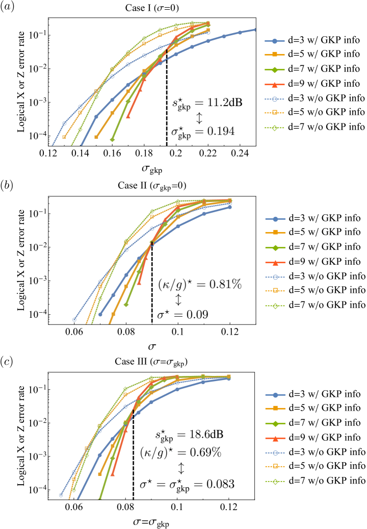
Figure 6: The logical $X$ error rate of the surface-GKP code for various $d$ when (a) $\sigma=0$ (Case I), (b) $\sigma_{\textrm{gkp}}=0$ (Case II), and (c) $\sigma=\sigma_{\textrm{gkp}}$ (Case III), which is the same as the logical $Z$ error rate. The solid lines represent logical error rates when information from the GKP-stabilizer measurements is used to renormalize edge weights in the matching graphs. The dotted lines correspond to the case when information from GKP-stabilizer measurements is ignored. In all cases, given that $\sigma_{\textrm{gkp}}$ and $\sigma$ are below certain fault-tolerance thresholds, the logical $X$ or $Z$ error rates are suppressed to an arbitrarily small value as we increase the code distance $d$.

In Fig. 6 (a), we consider the case where GKP states are the only noisy components in the scheme, i.e., $\sigma=0$ (Case I). We show the performance of the surface-GKP code when both the additional information from GKP-stabilizer measurements is incorporated and when it is ignored. When the additional information is incorporated, the logical $X$ error rate (same as the logical $Z$ error rate) decreases as we increase the code distance $d$ if $\sigma_{\textrm{gkp}}$ is smaller than the threshold value $\sigma_{\textrm{gkp}}^{\star}=0.194$ (or if the squeezing of the noisy GKP state $s_{\textrm{gkp}}$ is higher than the threshold value $s_{\textrm{gkp}}^{\star}=11.2$dB). That is, in this case, fault-tolerant error correction is possible with the surface-GKP code if the squeezing of the GKP states is above $11.2$dB. Note that if the additional information from GKP-stabilizer measurements is ignored, the threshold squeezing value decreases and logical error rates can range from one to several orders of magnitude larger for a given $\sigma_{\textrm{gkp}}$.

In Fig. 6 (b), we consider the case where GKP states are noiseless but the other circuit elements are noisy, i.e., $\sigma_{\textrm{gkp}}=0$ (Case II). In this case, if the additional information from the GKP error correction protocol is incorporated, we can suppress the logical $X$ error rate (same as the logical $Z$ error rate) to any desired small value by choosing a sufficiently large code distance $d$ as long as $\sigma$ is smaller than the threshold value $\sigma^{\star}=0.09$. Note that since $\sigma^{2}=\kappa/g$ the threshold value $\sigma^{\star}=0.09$ corresponds to $(\kappa/g)^{\star}=8.1\times 10^{-3}=0.81\%$, where $\kappa$ is the photon loss rate and $g$ is the coupling strength of the SUM or the inverse-SUM gates. That is, fault-tolerant error correction with the surface-GKP code is possible if the SUM or the inverse-SUM gates can be implemented roughly $120$ times faster than the photon loss processes. Note that if the additional information from GKP-stabilizer measurements is ignored, the threshold value becomes smaller and logical error rates can range from one to several orders of magnitude larger for a given $\sigma$.

Finally in Fig. 6 (c), we consider the case where the GKP states and the other circuit elements are comparably noisy, i.e., $\sigma=\sigma_{\textrm{gkp}}$ (Case III). In this case, fault-tolerant error correction is possible if $\sigma=\sigma_{\textrm{gkp}}$ is smaller than the threshold value $\sigma^{\star}=\sigma^{\star}_{\textrm{gkp}}=0.083$. This threshold value corresponds to the GKP squeezing $s_{\textrm{gkp}}^{\star}=18.6$dB and $\kappa/g=6.9\times 10^{-3}=0.69\%$. Similarly, as in the previous cases, if the additional information from GKP-stabilizer measurements is ignored, the threshold value becomes smaller and logical error rates can range from one to several orders of magnitude larger for a given noise parameter $\sigma=\sigma_{\textrm{gkp}}$.

For all three cases, we clearly observe that fault-tolerant quantum error correction with the surface-GKP code is possible despite noisy GKP states and noisy circuit elements, given that the noise parameters are below certain fault-tolerance thresholds. Recent state-of-the-art experiments have demonstrated the capability to prepare GKP states of squeezing between $5.5$dB and $9.5$dB Campagne-Ibarcq et al. (2019); Flühmann et al. (2018, 2019); Flühmann and Home (2019), approaching the established squeezing threshold values $s_{\textrm{gkp}}^{\star}\geq 11.2$dB.

In circuit QED systems, beam-splitter interactions between two high-Q cavity modes have been implemented experimentally with $\kappa/g\sim 10^{-2}$, where $g$ is the relevant coupling strength and $\kappa$ is the photon loss rate Gao et al. (2018). While the same scheme (based on four-wave mixing processes) may be adapted to realize the SUM or the inverse-SUM gates between two high-Q cavity modes Zhang et al. (2019), this scheme will induce non-negligible Kerr nonlinearities and thus may not be compatible with the GKP qubits which should be operated in the regime where Kerr nonlinearities are negligible Campagne-Ibarcq et al. (2019). On the other hand, by using three-wave mixing elements Frattini et al. (2017), it would be possible to implement the SUM or the inverse-SUM gates between two high-Q cavity modes in a way that is not significantly limited by Kerr nonlinearities.

Let us now compare the performance of the surface-GKP code with the usual rotated surface code implemented by bare qubits such as transmon qubits. Assuming a full circuit-level depolarizing noise (both for single- and two-qubit gates), it was numerically demonstrated that fault-tolerant quantum error correction is possible with the rotated surface code if the physical error rate is below the threshold $p^{\star}=1.2\%$ Wang et al. (2011). Note that such a high threshold value was obtained by introducing 3D space-time correlated edges (see Figs. 3 and 4 in Ref. Wang et al. (2011)) and fully optimizing the renormalized edge weights based on the noise parameters.

Our circuit-level noise model (in terms of shift errors) is quite different from the depolarizing noise model considered in typical qubit-based fault-tolerant error correction schemes. Moreover, we also introduce non-Gaussian resources, i.e., GKP states in our scheme. Therefore, our results cannot be directly compared with the results in Ref. Wang et al. (2011). We nevertheless point out that we obtain comparable threshold values $(\kappa/g)^{\star}=0.81\%$ (Case II) and $(\kappa/g)^{\star}=0.69\%$ (Case III) where $\kappa$ is the photon loss rate and $g$ is the coupling strength of the two-mode gates. We stress that we do not introduce 3D space-time correlated edges and provide a simple method for computing the renormalized edge weights. In particular, 3D space-time correlated edges are not necessary in our case with the surface-GKP code. This is because any shift errors that are correlated due to two-mode gates will not cause any Pauli errors to GKP qubits nor trigger syndrome GKP qubits incorrectly, as long as the size of the correlated shifts is smaller than $\sqrt{\pi}/2$, which is the case below the fault-tolerance thresholds computed above.

We also point out that in general, topological codes without leakage reduction units Aliferis and Terhal (2007) are not robust against leakage errors that occur when a bare qubit state is excited and falls out of its desired two-level subspace Aliferis and Terhal (2007); Fowler (2013); Suchara et al. (2015); Brown et al. (2019). In the case of the surface-GKP code, leakage errors do occur as well because each bosonic mode may not be in the desired two-level GKP code subspace. However, the surface-GKP code is inherently resilient to such leakage errors (and thus does not require leakage reduction units) since GKP-stabilizer measurements will detect and correct such events. Indeed, in our simulation of the surface-GKP code, leakage errors continuously occur due to shift errors, but the established fault-tolerance thresholds are nevertheless still favorable since GKP-stabilizer measurements prevent the leakage errors from propagating further.

We lastly remark that the logical $X$ or $Z$ error rates in Fig. 6 decrease very rapidly as $\sigma_{\textrm{gkp}}$ and $\sigma$ approach zero in the case of the surface-GKP code. This is again because the GKP code can correct any shift errors of size less than $\sqrt{\pi}/2$ and therefore the probability that a Pauli error occurs in a GKP qubit (at the end of GKP-stabilizer measurements) becomes exponentially small as $\sigma_{\textrm{gkp}}$ and $\sigma$ approach zero. More precisely, at the end of each GKP-stabilizer measurement, a bulk data GKP qubit undergoes a Pauli $X$ or $Z$ error with probability

$$p_{\textrm{err}}\Big{(}\sqrt{5\sigma_{\textrm{gkp}}^{2}+\frac{59}{3}\sigma^{2}}\Big{)},$$ (20)

where $p_{\textrm{err}}(\sigma)$ is defined in Eq. 10. Here, the variance $5\sigma_{\textrm{gkp}}^{2}+(59/3)\sigma^{2}$ was carefully determined by thoroughly keeping track of how circuit-level noise propagates during stabilizer measurements (see also Appendix B). As can be seen from Fig. 7, $p_{\textrm{err}}(\sigma)$ agrees well with the asymptotic expression $p_{\textrm{asy}}(\sigma)=(\sqrt{8}\sigma^{2}/\pi)\exp[-\pi/(8\sigma^{2})]$ in the $\sigma\ll 1$ limit. Thus, $p_{\textrm{err}}(\sigma)$ decreases exponentially as $\sigma$ goes to zero.

Similarly, the probability that a bulk surface code stabilizer measurement yields an incorrect measurement outcome is given by

$$p_{\textrm{err}}\Big{(}\sqrt{7\sigma_{\textrm{gkp}}^{2}+\frac{116}{3}\sigma^{2}}\Big{)},$$ (21)

and decays exponentially as $\sigma_{\textrm{gkp}}$ and $\sigma$ approach zero. Therefore, if the circuit-level noise of the physical bosonic modes is very small to begin with, GKP codes will locally provide a significant noise reduction. In this case, the overall resource overhead associated with the next level of global encoding will be modest since a small-distance surface code would suffice. Therefore in this regime, the surface-GKP code may be able to achieve the same target logical error rate in a more hardware-efficient way than the usual surface code. However, since this regime requires high quality GKP states, the additional resource overhead associated with the preparation of such high quality GKP states should also be taken into account for a comprehensive resource estimate. We leave such an analysis to future work.

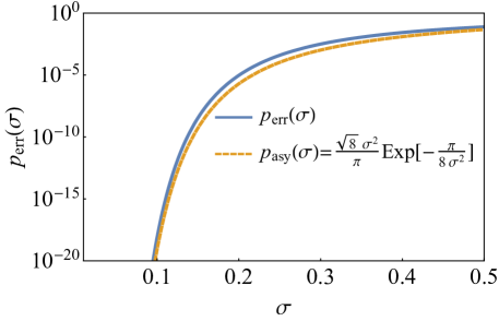
Figure 7: Visualization of the function $p_{\textrm{err}}(\sigma)$ (blue). The asymptotic expression $p_{\textrm{asy}}(\sigma)=(\sqrt{8}\sigma^{2}/\pi)\exp[-\pi/(8\sigma^{2})]$ is represented by the yellow dashed line. $p_{\textrm{err}}(\sigma)$ and $p_{\textrm{asy}}(\sigma)$ agree well with each other in the $\sigma\ll 1$ limit.

IV Discussion and outlook

3 Case I ($\sigma=0$)	Method	$\sigma_{\textrm{gkp}}^{\star}$	$s_{\textrm{gkp}}^{\star}$	Post-selection?	Success probability
3 Ref. Menicucci (2014)	Concatenated codes (MB)	$0.067$	$20.5$dB	NO	$1$
1.5 Ref. Fukui et al. (2018b)	3D cluster state (MB)	$0.228$	$9.8$dB	YES	decreases exponentially with $d^{3}$
1.5 Ref. Fukui (2019)	3D cluster state (MB)	$0.273$	$8.3$dB	YES	decreases exponentially with $d^{3}$
1.5 Refs. Wang (2017); Vuillot et al. (2019)	Toric-GKP code (GB)	N/A	N/A	NO	1
1.5 Our work	Surface-GKP code (GB)	$0.194$	$11.2$dB	NO	1
3

Table 1: Threshold values for the squeezing of GKP states for fault-tolerant quantum error correction. Here, we compare the established threshold values obtained by assuming that GKP states are the only noisy components in the error correction circuit (i.e., Case I). MB stands for measurement-based and GB stands for gate-based. $d$ is the distance of the code. For Refs. Wang (2017); Vuillot et al. (2019), $\sigma_{\textrm{gkp}}^{\star}$ and $s_{\textrm{gkp}}^{\star}$ are not available because they assumed phenomenological noise models that do not take into account the propagation of shift errors through the entire error correction circuit. That is, the threshold values established in Ref. Vuillot et al. (2019) using the toric-GKP code (i.e., $\sigma_{0}^{\star}=0.235$ and $\sigma_{0}^{\star}=0.243$ see Fig. 12 therein) do not accurately quantify the tolerable noise in the ancilla GKP states. Instead, $\sigma_{0}^{\star}$ can only be taken as a rough upper bound on $\sigma_{\textrm{gkp}}^{\star}$ (see the main text for more details).

Here, we compare the results obtained in this paper with previous works in Menicucci (2014); Wang (2017); Fukui et al. (2018b); Fukui (2019); Vuillot et al. (2019). Firstly, Refs. Wang (2017); Vuillot et al. (2019) considered the toric-GKP code and computed fault-tolerance thresholds for both code capacity and phenomenological noise models. In particular, the phenomenological noise models used in these works describe faulty syndrome extraction procedures (due to finitely-squeezed ancilla GKP states) in a way that does not take into account the propagation of the relevant shift errors. More specifically, in Figs. 1, 2, and 7 in Ref. Vuillot et al. (2019), shift errors are manually added in the beginning of each stabilizer measurement measurement and right before each homodyne measurement. Therefore, this phenomenological noise model can be understood as a model for homodyne detection inefficiencies while assuming ideal ancilla GKP states. In other words, the fault-tolerance threshold values established in Ref. Vuillot et al. (2019) (i.e., $\sigma_{0}^{\star}=0.235$ and $\sigma_{0}^{\star}=0.243$; see Fig. 12 therein) do not accurately represent the tolerable noise in the ancilla GKP states since the noise propagation was not thoroughly taken into account. Thus, these threshold values can only be taken as a rough upper bound on $\sigma_{\textrm{gkp}}^{\star}$ and cannot be directly compared with the threshold values obtained in our work. Note also that the threshold values in Ref. Vuillot et al. (2019) were computed for the toric code which has a different threshold compared to the rotated surface code Fowler et al. (2012).

On the other hand, in our work we assume that every GKP state supplied to the error correction chain has a finite squeezing and we comprehensively take into account the propagation of such shift errors through the entire error correction circuit. By doing so, we accurately estimate the tolerable noise in the finitely-squeezed ancilla GKP states by computing $\sigma_{\textrm{gkp}}^{\star}$. Related, we stress that when the noise propagation is taken into account, detailed scheduling and design of the syndrome extraction circuits become very crucial and we carefully designed the circuits in a way that mitigates the adverse effects of the noise propagation (see Fig. 5).

Moreover, we also consider photon loss and heating errors occurring continuously during the implementation of the SUM and inverse-SUM gates. Thus, we establish fault-tolerance thresholds for the strength of the two-mode coupling relative to the photon loss rate and demonstrate that fault-tolerant quantum error correction with the surface-GKP code is possible in more general scenarios. We also remark that Ref. Vuillot et al. (2019) used a minimum-energy decoder based on statistical-mechanical methods in the noisy regime whereas we provide a simple method for computing renormalized edge weights to be used in a MWPM decoder.

Secondly, Refs. Menicucci (2014); Fukui et al. (2018b); Fukui (2019) considered measurement-based quantum computing with GKP qubits and did establish fault-tolerance thresholds for the squeezing of the GKP states. Assuming that GKP states are the only noisy components (i.e., Case I), Ref. Menicucci (2014) found the squeezing threshold value $s_{\textrm{gkp}}^{\star}=20.5$dB, and Refs. Fukui et al. (2018b) and Fukui (2019) later brought the value down to $s_{\textrm{gkp}}^{\star}=9.8$dB and $s_{\textrm{gkp}}^{\star}=8.3$dB, respectively. Notably, the squeezing thresholds found in Refs. Fukui et al. (2018b); Fukui (2019) are more favorable than the squeezing threshold found in our work, i.e., $s_{\textrm{gkp}}^{\star}=11.2$dB (see Fig. 6 (a)). In this regard, we remark that the favorable threshold values obtained in Refs. Fukui et al. (2018b); Fukui (2019) rely on the use of post-selection. That is, each GKP measurement succeeds with probability strictly less than unity and thus the overall success probability would decrease exponentially as the system size $d$ increases. On the other hand, we do not discard any measurement outcomes and thus our scheme succeeds with unit probability for any distance $d$. Therefore, our scheme with the surface-GKP code deterministically suppresses errors exponentially with the code distance as long as $\sigma_{\textrm{gkp}}$ and $\sigma$ are below the threshold values. The differences between our work and the previous works are summarized in Table 1.

Let us now consider the number of bosonic modes needed to implement the distance-$d$ surface-GKP code: Recall Fig. 3 and note that we use $d^{2}$ data modes (white circles in Fig. 3), $d^{2}$ ancilla modes (grey circles in Fig. 3), and $d^{2}-1$ syndrome modes (green and orange circles in Fig. 3). Although we introduced the $d^{2}$ ancilla modes to describe our scheme in a simpler way, the $d^{2}$ ancilla modes can in fact be replaced by the $d^{2}-1$ syndrome qubits plus one more additional mode. Thus, we only need a total of $2d^{2}$ modes and geometrically local two-mode couplings to implement the distance-$d$ surface-GKP code. For example, $18$ modes would suffice to realize the smallest non-trivial case with $d=3$.

We finally emphasize that we modeled noisy GKP states by applying an incoherent random displacement error $\mathcal{N}[\sigma_{\textrm{gkp}}]$ to the ideal GKP states, similarly as in Refs. Menicucci (2014); Fukui et al. (2018b); Fukui (2019). While we use this noise model for theoretical convenience and justify it by using a twirling argument (see Appendix A), similar to the justification of a depolarizing error model in qubit-based QEC, we remark that it is not practical to use the twirling operation in realistic situations. This is because the twirling operation increases the average photon number of the GKP states, whereas in practice it is desirable to keep the photon number bounded below a certain cutoff. Therefore, an interesting direction for future work would be to see if one can implement the stabilizer measurements in Figs. 1, 3 and 4 in a manner that prevents the average photon number from diverging as we repeat the stabilizer measurements. It will be especially crucial to keep the average photon number under control when each bosonic mode suffers from dephasing errors and/or undesired nonlinear interactions such as Kerr nonlinearities.

Related, we remark that in the recent experimental realization of the GKP code in a circuit QED system, an envelope-trimming technique was used to constrain the average photon number of the system Campagne-Ibarcq et al. (2019). Whether a similar technique can be incorporated in a large-scale surface-GKP code architecture would be an interesting future research direction.

To summarize, we have thoroughly investigated the performance of the surface-GKP code assuming a detailed circuit-level noise model. By simulating the full noisy error correction protocol and using a minimum-weight perfect matching decoding on a 3D space-time graph (with a simple method for computing renormalized edge weights), we numerically demonstrated that fault-tolerant quantum error correction is possible with the surface-GKP code if the squeezing of the GKP states and the circuit noise are below certain fault-tolerance thresholds. Since our scheme does not require any post-selection and thus succeeds with unit probability, our scheme is clearly scalable. We also described our methods in great detail such that our results can easily be reproduced.

Appendix A Supplementary material for the noise model

To derive Eq. 15, we used the following identity.

$$\textrm{Tr}\big{[}\exp[-\Delta\hat{n}]\hat{D}^{\dagger}(\alpha)\big{]}$$

$$=\sum_{n=0}^{\infty}e^{-\Delta n}\langle n|\hat{D}^{\dagger}(\alpha)|n\rangle$$

$$=\exp\Big{[}-\frac{|\alpha|^{2}}{2}\Big{]}\sum_{n=0}^{\infty}e^{-\Delta n}L_{n}(|\alpha|^{2})$$

$$=\exp\Big{[}-\frac{|\alpha|^{2}}{2}\Big{]}\frac{1}{1-e^{-\Delta}}\exp\Big{[}-\frac{e^{-\Delta}}{1-e^{-\Delta}}|\alpha|^{2}\Big{]}$$

$$=\frac{1}{1-e^{-\Delta}}\exp\Big{[}-\frac{1+e^{-\Delta}}{2(1-e^{-\Delta})}|\alpha|^{2}\Big{]},$$ (22)

where $L_{n}(x)$ is the Laguerre polynomial. Further, going from the third to fourth line, we used the generating function for the Laguerre polynomials which satisfies $\sum_{n=0}^{\infty}t^{n}L_{n}(x)=\frac{1}{1-t}e^{-tx/(1-t)}$.

Now, we explain how one can transform the noisy GKP state corrupted by coherent superpositions of displacement errors (see Eq. 15) into the a noisy GKP state corrupted by an incoherent mixture of displacement errors (see Eq. 16). To do so, we apply random shifts of integer multiples $2\sqrt{\pi}$ in both the position and the momentum directions to the noisy GKP state $|\psi^{\Delta}_{\textrm{gkp}}\rangle\propto\exp[-\Delta\hat{n}]|\psi_{\textrm{gkp}}\rangle$. Then, $|\psi^{\Delta}_{\textrm{gkp}}\rangle$ is transformed into

$$\hat{\psi}_{\textrm{gkp}}^{\Delta} \propto\sum_{n_{1},n_{2}\in\mathbb{Z}}(\hat{S}_{q})^{n_{1}}(\hat{S}_{p})^{n_{2}}|\psi^{\Delta}_{\textrm{gkp}}\rangle\langle\psi_{\textrm{gkp}}^{\Delta}|(\hat{S}_{p}^{\dagger})^{n_{2}}(\hat{S}_{q}^{\dagger})^{n_{1}}$$

$$\propto\sum_{n_{1},n_{2}\in\mathbb{Z}}\int d^{2}\alpha d^{2}\beta\exp\Big{[}-\frac{|\alpha|^{2}+|\beta|^{2}}{2\sigma_{\textrm{gkp}}^{2}}\Big{]}(\hat{S}_{q})^{n_{1}}(\hat{S}_{p})^{n_{2}}\hat{D}(\alpha)|\psi_{\textrm{gkp}}\rangle\langle\psi_{\textrm{gkp}}|\hat{D}^{\dagger}(\beta)(\hat{S}_{p}^{\dagger})^{n_{2}}(\hat{S}_{q}^{\dagger})^{n_{1}}$$

$$\propto\sum_{n_{1},n_{2}\in\mathbb{Z}}\int d^{2}\alpha d^{2}\beta\exp\Big{[}-\frac{|\alpha|^{2}+|\beta|^{2}}{2\sigma_{\textrm{gkp}}^{2}}\Big{]}\exp[i\sqrt{2\pi}(\alpha_{R}-\beta_{R})n_{1}-i\sqrt{2\pi}(\alpha_{I}-\beta_{I})n_{2}]$$

$$\qquad\qquad\qquad\qquad\qquad\qquad\qquad\qquad\qquad\times\hat{D}(\alpha)(\hat{S}_{q})^{n_{1}}(\hat{S}_{p})^{n_{2}}|\psi_{\textrm{gkp}}\rangle\langle\psi_{\textrm{gkp}}|(\hat{S}_{p}^{\dagger})^{n_{2}}(\hat{S}_{q}^{\dagger})^{n_{1}}\hat{D}^{\dagger}(\beta)$$

$$\propto\sum_{n_{1},n_{2}\in\mathbb{Z}}\int d^{2}\alpha d^{2}\beta\exp\Big{[}-\frac{|\alpha|^{2}+|\beta|^{2}}{2\sigma_{\textrm{gkp}}^{2}}\Big{]}\exp[i\sqrt{2\pi}(\alpha_{R}-\beta_{R})n_{1}-i\sqrt{2\pi}(\alpha_{I}-\beta_{I})n_{2}]\hat{D}(\alpha)|\psi_{\textrm{gkp}}\rangle\langle\psi_{\textrm{gkp}}|\hat{D}^{\dagger}(\beta),$$ (23)

where we used the identity $\hat{D}(\alpha)\hat{D}(\beta)=\hat{D}(\beta)\hat{D}(\alpha)e^{\alpha\beta^{*}-\alpha^{*}\beta}$ and the fact that GKP states are stabilized by the GKP stabilizers $\hat{S}_{q}=\hat{D}(i\sqrt{2\pi})$ and $\hat{S}_{p}=\hat{D}(\sqrt{2\pi})$, i.e., $\hat{S}_{q}|\psi_{\textrm{gkp}}\rangle=\hat{S}_{p}|\psi_{\textrm{gkp}}\rangle=|\psi_{\textrm{gkp}}\rangle$. Using the Poisson summation formula, $\sum_{n\in\mathbb{Z}}e^{ian}=2\pi\sum_{k\in\mathbb{Z}}\delta(a-2\pi k)$ we can further simplify Eq. 23 as

$$\hat{\psi}_{\textrm{gkp}}^{\Delta} \propto\sum_{k_{1},k_{2}\in\mathbb{Z}}\int d^{2}\alpha d^{2}\beta\exp\Big{[}-\frac{|\alpha|^{2}+|\beta|^{2}}{2\sigma_{\textrm{gkp}}^{2}}\Big{]}\delta(\alpha_{R}-\beta_{R}-\sqrt{2\pi}k_{1})\delta(\alpha_{I}-\beta_{I}-\sqrt{2\pi}k_{2})\hat{D}(\alpha)|\psi_{\textrm{gkp}}\rangle\langle\psi_{\textrm{gkp}}|\hat{D}^{\dagger}(\beta)$$

$$=\sum_{k_{1},k_{2}\in\mathbb{Z}}\int d^{2}\alpha\exp\Big{[}-\frac{|\alpha|^{2}+|\alpha-\sqrt{2\pi}(k_{1}+ik_{2})|^{2}}{2\sigma_{\textrm{gkp}}^{2}}\Big{]}\hat{D}(\alpha)|\psi_{\textrm{gkp}}\rangle\langle\psi_{\textrm{gkp}}|\hat{D}^{\dagger}(\alpha-\sqrt{2\pi}(k_{1}+ik_{2}))$$

$$=\sum_{k_{1},k_{2}\in\mathbb{Z}}\exp\Big{[}-\frac{\pi|k_{1}+ik_{2}|^{2}}{2\sigma_{\textrm{gkp}}^{2}}\Big{]}\int d^{2}\alpha\exp\Big{[}-\frac{|\alpha-\sqrt{\frac{\pi}{2}}(k_{1}+ik_{2})|^{2}}{\sigma_{\textrm{gkp}}^{2}}\Big{]}\hat{D}(\alpha)|\psi_{\textrm{gkp}}\rangle\langle\psi_{\textrm{gkp}}|\hat{D}^{\dagger}(\alpha-\sqrt{2\pi}(k_{1}+ik_{2})).$$ (24)

Lastly, if $\sigma_{\textrm{gkp}}\ll\sqrt{\pi}$ (which is the case below the fault-tolerance threshold $\sigma_{\textrm{gkp}}^{\star}\leq 0.194$), we can neglect all the $(k_{1},k_{2})\neq(0,0)$ terms due to the exponentially decaying prefactor $\exp[-\frac{\pi|k_{1}+ik_{2}|^{2}}{2\sigma_{\textrm{gkp}}^{2}}]$ and get the noise model in Eq. 16:

$$\hat{\psi}_{\textrm{gkp}}^{\Delta} \propto\int\frac{d^{2}\alpha}{\pi\sigma_{\textrm{gkp}}^{2}}\exp\Big{[}-\frac{|\alpha|^{2}}{\sigma_{\textrm{gkp}}^{2}}\Big{]}\hat{D}(\alpha)|\psi_{\textrm{gkp}}\rangle\langle\psi_{\textrm{gkp}}|\hat{D}^{\dagger}(\alpha)=\mathcal{N}[\sigma_{\textrm{gkp}}](|\psi_{\textrm{gkp}}\rangle\langle\psi_{\textrm{gkp}}|).$$ (25)

Let us now derive the gate error model given in Eq. 19. Recall that $\mathcal{L}^{\prime}_{\pm}$ is given by

$$\mathcal{L}^{\prime}_{\pm}=\mathcal{V}_{\pm}+\mathcal{L}_{\textrm{err}},$$ (26)

where $\mathcal{V}_{\pm}$ and $\mathcal{L}_{\textrm{err}}$ are defined as

$$\mathcal{V}_{\pm}(\hat{\rho}) \equiv\mp ig[\hat{q}_{1}\hat{p}_{2},\hat{\rho}],$$

$$\mathcal{L}_{\textrm{err}}(\hat{\rho}) \equiv\kappa\sum_{k=1}^{2}\big{(}\mathcal{D}[\hat{a}_{k}]+\mathcal{D}[\hat{a}^{\dagger}_{k}]\big{)}\hat{\rho}.$$ (27)

The noisy SUM or the inverse-SUM gates is then given by $\exp[\mathcal{L}^{\prime}_{\pm}\Delta t]$ with $\Delta t=1/g$. Note that Trotter’s formula Trotter (1959) yields

$$\exp[\mathcal{L}^{\prime}_{\pm}\Delta t] =\lim_{N\rightarrow\infty}\Big{[}\exp\Big{[}\mathcal{V}_{\pm}\frac{\Delta t}{N}\Big{]}\exp\Big{[}\mathcal{L}_{\textrm{err}}\frac{\Delta t}{N}\Big{]}\Big{]}^{N}.$$ (28)

Note that both $\exp[\mathcal{V}_{\pm}\Delta t/N]$ and $\exp[\mathcal{L}_{\textrm{err}}\Delta t/N]$ are Gaussian channels with the characterization matrices

$$\bm{T}_{\pm} =\begin{bmatrix}1&0&0&0\\ 0&1&0&\mp 1/N\\ \pm 1/N&0&1&0\\ 0&0&0&1\end{bmatrix},\quad\bm{N}_{\pm}=0,$$

$$\bm{T}_{\textrm{err}} =\begin{bmatrix}1&0&0&0\\ 0&1&0&0\\ 0&0&1&0\\ 0&0&0&1\end{bmatrix},\quad\bm{N}_{\textrm{err}}=\frac{\kappa\Delta t}{N}\begin{bmatrix}1&0&0&0\\ 0&1&0&0\\ 0&0&1&0\\ 0&0&0&1\end{bmatrix},$$ (29)

respectively (see, for example, Ref. Weedbrook et al. (2012) for the definition of Gaussian channels and their characterization matrices). Thus, the quadrature operator $\bm{\hat{x}}=(\hat{q}_{1},\hat{p}_{1},\hat{q}_{2},\hat{p}_{2})^{T}$ is transformed via the noisy SUM or the inverse-SUM gate as

$$\bm{\hat{x}} \rightarrow(\bm{T}_{\pm})^{N}\bm{\hat{x}}=\begin{bmatrix}1&0&0&0\\ 0&1&0&\mp 1\\ \pm 1&0&1&0\\ 0&0&0&1\end{bmatrix}\bm{\hat{x}}=\begin{bmatrix}\hat{q}_{1}\\ \hat{p}_{1}\mp\hat{p}_{2}\\ \hat{q}_{2}\pm\hat{q}_{1}\\ \hat{p}_{2}\end{bmatrix},$$ (30)

as desired. Also, the covariance matrix $\bm{V}$ is transformed as

$$\bm{V} \rightarrow(\bm{T}_{\pm})^{N}\bm{V}((\bm{T}_{\pm})^{N})^{T}+\sum_{k=1}^{N}(\bm{T}_{\pm})^{k}\bm{N}_{\textrm{err}}(\bm{T}_{\pm}^{T})^{k}$$

$$=(\bm{T}_{\pm})^{N}\bm{V}((\bm{T}_{\pm})^{N})^{T}$$

$$\quad+\sum_{k=1}^{N}\frac{\kappa\Delta t}{N}\begin{bmatrix}1&0&\pm\frac{k}{N}&0\\ 0&1+(\frac{k}{N})^{2}&0&\mp\frac{k}{N}\\ \pm\frac{k}{N}&0&1+(\frac{k}{N})^{2}&0\\ 0&\mp\frac{k}{N}&0&1\end{bmatrix}$$

$$=(\bm{T}_{\pm})^{N}\bm{V}((\bm{T}_{\pm})^{N})^{T}$$

$$\quad+\kappa\Delta t\begin{bmatrix}1&0&\pm 1/2&0\\ 0&4/3&0&\mp 1/2\\ \pm 1/2&0&4/3&0\\ 0&\mp 1/2&0&1\end{bmatrix}.$$ (31)

Therefore, the noisy SUM or the inverse-SUM gate can be understood as the ideal SUM or the inverse-SUM gate followed by a correlated Gaussian random displacement error with the noise covariance matrices $\bm{N}_{q}^{\pm}$ and $\bm{N}_{p}^{\pm}$ as given in Eq. 19.

Appendix B Simulation details

Here, we describe in detail how we simulate the syndrome extraction protocol for the surface-GKP code and how we decode the obtained syndrome measurement outcome.

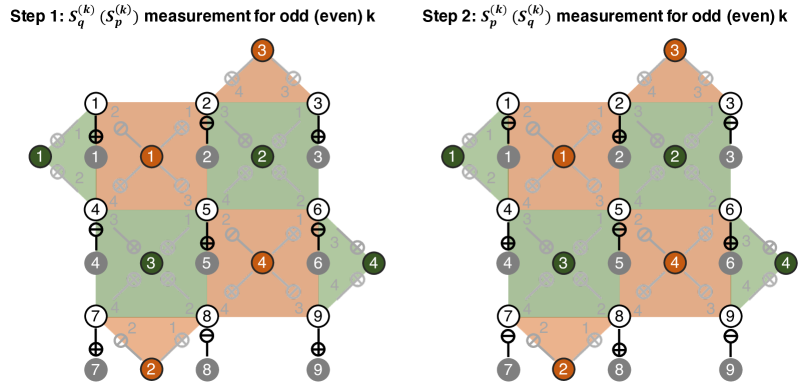
Figure 8: Measurement of the GKP stabilizers for $d=3$. See also Fig. 1 (b) for the graphical notation.

GKP-stabilizer measurements

Consider the distance-$d$ surface-GKP code consisting of $d^{2}$ data GKP qubits. Each data GKP qubit is stabilized by the two GKP stabilizers $\hat{S}_{q}^{(k)}=\exp[i2\sqrt{\pi}\hat{q}_{k}]$ and $\hat{S}_{p}^{(k)}=\exp[-i2\sqrt{\pi}\hat{p}_{k}]$ where $k\in\{1,\cdots,d^{2}\}$. In the first step of GKP-stabilizer measurements (left in Fig. 8), $\hat{S}_{q}^{(k)}$ ($\hat{S}_{p}$) stabilizers are measured for odd (even) $k$. In the second step (right in Fig. 8), on the other hand, $\hat{S}_{p}^{(k)}$ ($\hat{S}_{q}^{(k)}$) stabilizers are measured for odd (even) $k$. Note that we alternate between $\hat{S}_{q}$ and $\hat{S}_{p}$ measurements in a checkerboard pattern in order to balance the position and momentum quadrature noise.

Let $\xi_{q}^{D}$ and $\xi_{p}^{D}$ ($\xi_{q}^{A}$ and $\xi_{p}^{A}$) be the data (ancilla) position and momentum quadrature noise, where

$$\xi_{q}^{D} =(\xi_{q}^{(D1)},\cdots,\xi_{q}^{(Dd^{2})}),$$

$$\xi_{p}^{D} =(\xi_{p}^{(D1)},\cdots,\xi_{p}^{(Dd^{2})}),$$

$$\xi_{q}^{A} =(\xi_{q}^{(A1)},\cdots,\xi_{q}^{(Ad^{2})}),$$

$$\xi_{p}^{A} =(\xi_{p}^{(A1)},\cdots,\xi_{p}^{(Ad^{2})}).$$ (32)

In Step 1, we add random shift errors occurring during the GKP state preparation as follows:

$$\xi_{q}^{(Dk)} \leftarrow\xi_{q}^{(Dk)}+\textrm{randG}(\sigma^{2}),$$

$$\xi_{p}^{(Dk)} \leftarrow\xi_{p}^{(Dk)}+\textrm{randG}(\sigma^{2}),$$

$$\xi_{q}^{(Ak)} \leftarrow\textrm{randG}(\sigma_{\textrm{gkp}}^{2}),$$

$$\xi_{p}^{(Ak)} \leftarrow\textrm{randG}(\sigma_{\textrm{gkp}}^{2}),$$ (33)

for $k\in\{1,\cdots,d^{2}\}$ where $\textrm{randG}(\bm{V})$ generates a random vector sampled from a multivariate Gaussian distribution $\mathcal{N}(0,\bm{V})$ with zero mean and the covariance matrix $\bm{V}$. Then, due to the SUM and the inverse-SUM gates, the quadrature noise vectors are updated as follows.

$$(\xi_{q}^{(Dk)},\xi_{q}^{(Ak)}) \leftarrow(\xi_{q}^{(Dk)},\xi_{q}^{(Ak)}+\xi_{q}^{(Dk)})$$

$$\qquad+\textrm{randG}\Big{(}\sigma^{2}\begin{bmatrix}1&1/2\\ 1/2&4/3\end{bmatrix}\Big{)},$$

$$(\xi_{p}^{(Dk)},\xi_{p}^{(Ak)}) \leftarrow(\xi_{p}^{(Dk)}-\xi_{p}^{(Ak)},\xi_{p}^{(Ak)})$$

$$\qquad+\textrm{randG}\Big{(}\sigma^{2}\begin{bmatrix}4/3&-1/2\\ -1/2&1\end{bmatrix}\Big{)},$$ (34)

for odd $k$ ($\hat{S}_{q}^{(k)}$ stabilizer measurement) and

$$(\xi_{q}^{(Dk)},\xi_{q}^{(Ak)}) \leftarrow(\xi_{q}^{(Dk)}-\xi_{q}^{(Ak)},\xi_{q}^{(Ak)})$$

$$\qquad+\textrm{randG}\Big{(}\sigma^{2}\begin{bmatrix}4/3&-1/2\\ -1/2&1\end{bmatrix}\Big{)},$$

$$(\xi_{p}^{(Dk)},\xi_{p}^{(Ak)}) \leftarrow(\xi_{p}^{(Dk)},\xi_{p}^{(Ak)}+\xi_{p}^{(Dk)})$$

$$\qquad+\textrm{randG}\Big{(}\sigma^{2}\begin{bmatrix}1&1/2\\ 1/2&4/3\end{bmatrix}\Big{)},$$ (35)

for even $k$ ($\hat{S}_{p}^{(k)}$ stabilizer measurement). Due to the noise before (or during) the homodyne measurement, the noise vectors are updated as

$$\xi_{q}^{(Dk)} \leftarrow\xi_{q}^{(Dk)}+\textrm{randG}(\sigma^{2}),$$

$$\xi_{p}^{(Dk)} \leftarrow\xi_{p}^{(Dk)}+\textrm{randG}(\sigma^{2}),$$

$$\xi_{q}^{(Ak)} \leftarrow\xi_{q}^{(Ak)}+\textrm{randG}(\sigma^{2}),$$

$$\xi_{p}^{(Ak)} \leftarrow\xi_{p}^{(Ak)}+\textrm{randG}(\sigma^{2}),$$ (36)

for all $k\in\{1,\cdots,d^{2}\}$. Then, through the homodyne measurement and the error correction process, the data noise vectors are transformed as

$$\xi_{q}^{(Dk)}\leftarrow\xi_{q}^{(Dk)}-R_{\sqrt{\pi}}\big{(}\xi_{q}^{(Ak)}\big{)},$$ (37)

$$\xi_{p}^{(Dk)}\leftarrow\xi_{p}^{(Dk)}-R_{\sqrt{\pi}}\big{(}\xi_{p}^{(Ak)}\big{)},$$ (38)

for odd and even $k$, respectively. $R_{s}(z)$ is defined as

$$R_{s}(z)\equiv z-s\Big{\lfloor}\frac{z}{s}+\frac{1}{2}\Big{\rfloor}.$$ (39)

In Step 2, $\hat{S}_{p}^{(k)}$ ($\hat{S}_{q}^{(k)}$) stabilizers are measured for odd (even) $k$ instead of $\hat{S}_{q}^{(k)}$ ($\hat{S}_{p}^{(k)}$). Thus, the noise vectors are updated similarly as in Eqs. 33, 34, 35, 36, 37 and 38, except that Eqs. 34 and 37 (Eqs. 35 and 38) are applied when $k$ is even (odd) instead of when $k$ is odd (even).

Surface code stabilizer measurements

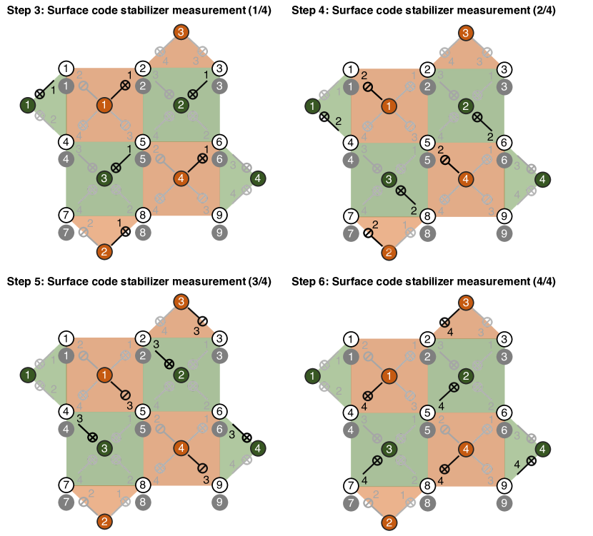
Figure 9: Measurement of the surface code stabilizers for $d=3$.

Recall that there are $d^{\prime}\equiv(d^{2}-1)/2$ $Z$-type and $X$-type syndrome GKP qubits that are used to measure the surface code stabilizers. Let $\xi_{q}^{Z}$ and $\xi_{p}^{Z}$ ($\xi_{q}^{X}$ and $\xi_{p}^{X}$) be the position and momentum noise vectors of the $Z$-type ($X$-type) syndrome GKP qubits, where

$$\xi_{q}^{Z} =(\xi_{q}^{(Z1)},\cdots,\xi_{q}^{(Zd^{\prime})}),$$

$$\xi_{p}^{Z} =(\xi_{p}^{(Z1)},\cdots,\xi_{p}^{(Zd^{\prime})}),$$

$$\xi_{q}^{X} =(\xi_{q}^{(X1)},\cdots,\xi_{q}^{(Xd^{\prime})}),$$

$$\xi_{p}^{X} =(\xi_{p}^{(X1)},\cdots,\xi_{p}^{(Xd^{\prime})}).$$ (40)

Note that the SUM and the inverse-SUM gates for the syndrome extraction are executed in four time steps (see Steps 3,4,5,6 in Fig. 9). Let $Z_{1}(k),\cdots,Z_{4}(k)$ ($X_{1}(k),\cdots,X_{4}(k)$) be the label of the data GKP qubit that the $k^{\textrm{th}}$ $Z$-type ($X$-type) syndrome GKP qubit is coupled with in Steps $3,\cdots,6$. (If the syndrome GKP qubit is idling, the value is set to be zero). For example when $d=3$, $Z_{1}(k)$ and $X_{1}(k)$ are given by

$$Z_{1}(1)=1,\,\, Z_{1}(2) =3,\,\, Z_{1}(3) =5,\,\, Z_{1}(4) =0,$$

$$X_{1}(1)=2,\,\, X_{1}(2) =0,\,\, X_{1}(3) =8,\,\, X_{1}(4) =6,$$ (41)

representing the connectivity between the syndrome and the data GKP qubits in Step 3.

Due to the shift errors occurring during the preparation of GKP states, the noise vectors are updated as follows:

$$\xi_{q}^{(Dk)} \leftarrow\xi_{q}^{(Dk)}+\textrm{randG}(\sigma^{2}),$$

$$\xi_{p}^{(Dk)} \leftarrow\xi_{p}^{(Dk)}+\textrm{randG}(\sigma^{2}),$$

$$\xi_{q}^{(Z\ell)} \leftarrow\textrm{randG}(\sigma_{\textrm{gkp}}^{2}),$$

$$\xi_{p}^{(Z\ell)} \leftarrow\textrm{randG}(\sigma_{\textrm{gkp}}^{2}),$$

$$\xi_{q}^{(X\ell)} \leftarrow\textrm{randG}(\sigma_{\textrm{gkp}}^{2}),$$

$$\xi_{p}^{(X\ell)} \leftarrow\textrm{randG}(\sigma_{\textrm{gkp}}^{2}),$$ (42)

for $k\in\{1,\cdots,d^{2}\}$ and $\ell\in\{1,\cdots,d^{\prime}\}$. In Step 3, the SUM gates transform the noise vectors as

$$(\xi_{q}^{(DZ_{1}(\ell))},\xi_{q}^{(Z\ell)}) \leftarrow(\xi_{q}^{(DZ_{1}(\ell))},\xi_{q}^{(Z\ell)}+\xi_{q}^{(DZ_{1}(\ell))})$$

$$\qquad+\textrm{randG}\Big{(}\sigma^{2}\begin{bmatrix}1&1/2\\ 1/2&4/3\end{bmatrix}\Big{)},$$

$$(\xi_{p}^{(DZ_{1}(\ell))},\xi_{p}^{(Z\ell)}) \leftarrow(\xi_{p}^{(DZ_{1}(\ell))}-\xi_{p}^{(Z\ell)},\xi_{p}^{(Z\ell)})$$

$$\qquad+\textrm{randG}\Big{(}\sigma^{2}\begin{bmatrix}4/3&-1/2\\ -1/2&1\end{bmatrix}\Big{)},$$ (43)

for all $\ell\in\{1,\cdots,d^{\prime}\}$ if $Z_{1}(\ell)\neq 0$ and

$$\xi_{q}^{(Z\ell)} \leftarrow\xi_{q}^{(Z\ell)}+\textrm{randG}(\sigma^{2}),$$

$$\xi_{p}^{(Z\ell)} \leftarrow\xi_{p}^{(Z\ell)}+\textrm{randG}(\sigma^{2}),$$ (44)

if $Z_{1}(\ell)=0$. Similarly,

$$(\xi_{q}^{(DX_{1}(\ell))},\xi_{q}^{(X\ell)}) \leftarrow(\xi_{q}^{(DX_{1}(\ell))}+\xi_{q}^{(X\ell)},\xi_{q}^{(X\ell)})$$

$$\qquad+\textrm{randG}\Big{(}\sigma^{2}\begin{bmatrix}4/3&1/2\\ 1/2&1\end{bmatrix}\Big{)},$$

$$(\xi_{p}^{(DX_{1}(\ell))},\xi_{p}^{(X\ell)}) \leftarrow(\xi_{p}^{(DX_{1}(\ell))},\xi_{p}^{(X\ell)}-\xi_{p}^{(DX_{1}(\ell))})$$

$$\quad+\textrm{randG}\Big{(}\sigma^{2}\begin{bmatrix}1&-1/2\\ -1/2&4/3\end{bmatrix}\Big{)},$$ (45)

for all $\ell\in\{1,\cdots,d^{\prime}\}$ if $X_{1}(\ell)\neq 0$ and

$$\xi_{q}^{(X\ell)} \leftarrow\xi_{q}^{(X\ell)}+\textrm{randG}(\sigma^{2}),$$

$$\xi_{p}^{(X\ell)} \leftarrow\xi_{p}^{(X\ell)}+\textrm{randG}(\sigma^{2}),$$ (46)

if $X_{1}(\ell)=0$. Since there are idling data GKP qubits, the data noise vectors are updated as

$$\xi_{q}^{(Dk)} \leftarrow\xi_{q}^{(Dk)}+\textrm{randG}(\sigma^{2}),$$

$$\xi_{p}^{(Dk)} \leftarrow\xi_{p}^{(Dk)}+\textrm{randG}(\sigma^{2}),$$ (47)

only for $k$ such that $Z_{1}(\ell)\neq k$ and $X_{1}(\ell)\neq k$ for all $\ell\in\{1,\cdots,d^{\prime}\}$.

In Step 4, the SUM gates between the $Z$-type syndrome GKP qubits and data GKP qubits transform the noise vectors in the same way as in Eqs. 43 and 44 except that $Z_{1}(\ell)$ is replaced by $Z_{2}(\ell)$. However, since the $X$-type syndrome GKP qubits are coupled with the data GKP qubits through inverse-SUM gates instead of SUM gates, the noise vectors are then updated as

$$(\xi_{q}^{(DX_{2}(\ell))},\xi_{q}^{(X\ell)}) \leftarrow(\xi_{q}^{(DX_{2}(\ell))}-\xi_{q}^{(X\ell)},\xi_{q}^{(X\ell)})$$

$$\qquad+\textrm{randG}\Big{(}\sigma^{2}\begin{bmatrix}4/3&-1/2\\ -1/2&1\end{bmatrix}\Big{)},$$

$$(\xi_{p}^{(DX_{2}(\ell))},\xi_{p}^{(X\ell)}) \leftarrow(\xi_{p}^{(DX_{2}(\ell))},\xi_{p}^{(X\ell)}+\xi_{p}^{(DX_{2}(\ell))})$$

$$\quad+\textrm{randG}\Big{(}\sigma^{2}\begin{bmatrix}1&1/2\\ 1/2&4/3\end{bmatrix}\Big{)},$$ (48)

for all $\ell\in\{1,\cdots,d^{\prime}\}$ if $X_{2}(\ell)\neq 0$ and

$$\xi_{q}^{(X\ell)} \leftarrow\xi_{q}^{(X\ell)}+\textrm{randG}(\sigma^{2}),$$

$$\xi_{p}^{(X\ell)} \leftarrow\xi_{p}^{(X\ell)}+\textrm{randG}(\sigma^{2}),$$ (49)

if $X_{2}(\ell)=0$, instead of as in Eqs. 45 and 46. Due to the idling data GKP qubits, the noise vectors are further updated as in Eq. 47 only for $k$ such that $Z_{2}(\ell)\neq k$ and $X_{2}(\ell)\neq k$ for all $\ell\in\{1,\cdots,d^{\prime}\}$.

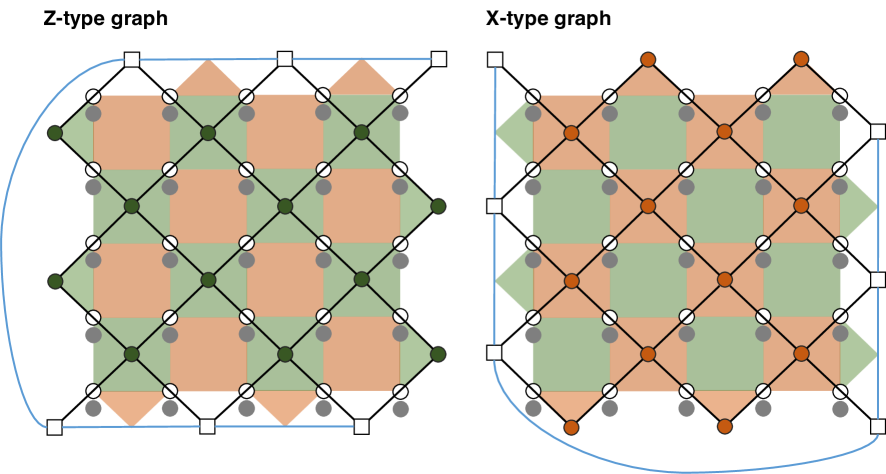
Figure 10: $Z$-type and $X$-type 2D space graphs for the surface-GKP code with $d=5$. These 2D graphs will be stacked up to construct $Z$-type and $X$-type 3D space-time graphs.

Note that in Step 5 and Step 6, the $X$-type syndrome GKP qubits are coupled with the data GKP qubits via inverse-SUM gates and SUM gates, respectively. Therefore, in Step 5, the noise vectors are updated in the same way as in Step 4, except that $Z_{2}(\ell)$ and $Z_{2}(\ell)$ are replaced by $Z_{3}(\ell)$ and $X_{3}(\ell)$. On the other hand, in Step 6, the noise vectors are updated in the same way as in Step 3, except that $Z_{1}(\ell)$ and $X_{1}(\ell)$ are replaced by $Z_{4}(\ell)$ and $X_{4}(\ell)$. Due to the noise before (or during) the homodyne measurement, the noise vectors are updated as

$$\xi_{q}^{(Dk)} \leftarrow\xi_{q}^{(Dk)}+\textrm{randG}(\sigma^{2}),$$

$$\xi_{p}^{(Dk)} \leftarrow\xi_{p}^{(Dk)}+\textrm{randG}(\sigma^{2}),$$

$$\xi_{q}^{(Z\ell)} \leftarrow\xi_{q}^{(Z\ell)}+\textrm{randG}(\sigma^{2}),$$

$$\xi_{p}^{(Z\ell)} \leftarrow\xi_{p}^{(Z\ell)}+\textrm{randG}(\sigma^{2}),$$

$$\xi_{q}^{(X\ell)} \leftarrow\xi_{q}^{(X\ell)}+\textrm{randG}(\sigma^{2}),$$

$$\xi_{p}^{(X\ell)} \leftarrow\xi_{p}^{(X\ell)}+\textrm{randG}(\sigma^{2}),$$ (50)

for all $k\in\{1,\cdots,d^{2}\}$ and $\ell\in\{1,\cdots,d^{\prime}\}$. Then, through the homodyne measurement, we measure $\xi_{q}^{(Z\ell)}$ and $\xi_{p}^{(X\ell)}$ modulo $2\sqrt{\pi}$ and assign stabilizer values as

$$\hat{S}_{Z}^{(\ell)} \leftarrow\begin{cases}+1&|R_{\sqrt{2\pi}}(\xi_{q}^{(Z\ell)})|\leq\sqrt{\pi}/2\\ -1&|R_{\sqrt{2\pi}}(\xi_{q}^{(Z\ell)})|>\sqrt{\pi}/2\end{cases},$$

$$\hat{S}_{X}^{(\ell)} \leftarrow\begin{cases}+1&|R_{\sqrt{2\pi}}(\xi_{p}^{(X\ell)})|\leq\sqrt{\pi}/2\\ -1&|R_{\sqrt{2\pi}}(\xi_{p}^{(X\ell)})|>\sqrt{\pi}/2\end{cases},$$ (51)

for all $\ell\in\{1,\cdots,d^{\prime}\}$. $R_{s}(z)$ is defined in Eq. 39.

Construction of 3D space-time graphs

Now we construct 3D space-time graphs to which we will apply a minimum-weight perfect matching decoding algorithm. The overall structure is as follows: Since each stabilizer measurement can be faulty, we repeat the noisy stabilizer measurement cycle $d$ times. Then, we perform another round of ideal stabilizer measurement cycle assuming that all circuit elements and supplied GKP states are noiseless. The reason for adding the extra noiseless measurement cycle is to ensure that the noisy states are restored back to the code space so we can later conveniently determine whether the error correction succeed or not. Then, the $Z$-type and the $X$-type 3D space-time graphs are constructed to represent the outcomes of $d+1$ rounds of stabilizer measurement cycles. These space-time graphs will then be used to decode the $Z$-type and the $X$-type syndrome measurement outcomes.

We first construct the $Z$-type and $X$-type 2D space graphs as in Fig. 10. Each bulk vertex of the 2D space graph corresponds to a syndrome GKP qubit and each bulk edge corresponds to a data GKP qubit. Note also that there are boundary vertices (squares in Fig. 10) that do not correspond to any syndrome GKP qubits and the corresponding boundary edges (blue lines in Fig. 10) that are not associated with any data GKP qubits. Therefore, the boundary edge weighs are always set to be zero.

Then, we associate each 2D space graph with one round of stabilizer measurement cycle. So, there are $d+1$ 2D space graphs and these 2D space graphs are stacked up together by introducing vertical edges that connect the same vertices in two adjacent 2D space graphs (corresponding to two adjacent stabilizer measurement rounds). Below, we discuss in detail how the bulk edge weights are assigned.

We start by initializing the data position and momentum noise vectors to a zero vector:

$$\xi_{q}^{D} =(\xi_{q}^{(D1)},\cdots,\xi_{q}^{(Dd^{2})})=(0,\cdots,0),$$

$$\xi_{p}^{D} =(\xi_{p}^{(D1)},\cdots,\xi_{p}^{(Dd^{2})})=(0,\cdots,0).$$ (52)

These data noise vectors are fed into Step 1 of GKP-stabilizer measurement as described in Eqs. 33, 34, 35 and 36. Let $w_{Z}^{H}(k)$ and $w_{Z}^{H}(k)$ be the horizontal edge weights of the $Z$-type and $X$-type graphs corresponding to the $k^{\textrm{th}}$ data GKP qubit ($k\in\{1,\cdots,d^{2}\}$). Then, while updating the data position and momentum noise vectors as prescribed in Eqs. 37 and 38, we assign the horizontal edge weights as

$$w_{Z}^{H}(k) \leftarrow\begin{cases}-\log_{2}\big{(}p[\sqrt{\sigma_{\textrm{gkp}}^{2}+\frac{10}{3}\sigma^{2}}]\big{(}R_{\sqrt{\pi}}(\xi_{q}^{(Ak)})\big{)}\big{)}&\textrm{round }1\\ -\log_{2}\big{(}p[\sigma_{Z}^{H}(k;d)]\big{(}R_{\sqrt{\pi}}(\xi_{q}^{(Ak)})\big{)}\big{)}&\textrm{round }2\textrm{ to round }d\\ -\log_{2}\big{(}p[\sqrt{(\sigma_{Z}^{H}(k;d))^{2}-\sigma_{\textrm{gkp}}^{2}-\frac{10}{3}\sigma^{2}}]\big{(}R_{\sqrt{\pi}}(\xi_{q}^{(Ak)})\big{)}\big{)}&\textrm{round }d+1\end{cases},$$ (53)

for odd $k$ and

$$w_{X}^{H}(k) \leftarrow\begin{cases}-\log_{2}\big{(}p[\sqrt{\sigma_{\textrm{gkp}}^{2}+\frac{10}{3}\sigma^{2}}]\big{(}R_{\sqrt{\pi}}(\xi_{p}^{(Ak)})\big{)}\big{)}&\textrm{round }1\\ -\log_{2}\big{(}p[\sigma_{X}^{H}(k;d)]\big{(}R_{\sqrt{\pi}}(\xi_{p}^{(Ak)})\big{)}\big{)}&\textrm{round }2\textrm{ to round }d\\ -\log_{2}\big{(}p[\sqrt{(\sigma_{X}^{H}(k;d))^{2}-\sigma_{\textrm{gkp}}^{2}-\frac{10}{3}\sigma^{2}}]\big{(}R_{\sqrt{\pi}}(\xi_{p}^{(Ak)})\big{)}\big{)}&\textrm{round }d+1\end{cases},$$ (54)

for even $k$ if the additional GKP information is used. Here, we use $\xi_{q}^{(Ak)}$ and $\xi_{p}^{(Ak)}$ that are obtained after applying Eq. 36. $p_{\textrm{err}}(\sigma)$ and $p[\sigma](z)$ are defined in Eqs. 10 and 11 and $R_{s}(z)$ is defined in Eq. 39. On the other hand, if the additional GKP information is not used, we assign the horizontal edge weights as

$$w_{Z}^{H}(k) \leftarrow\begin{cases}-\log_{2}\big{(}p_{\textrm{err}}\big{(}\sqrt{\sigma_{\textrm{gkp}}^{2}+\frac{10}{3}\sigma^{2}}\big{)}\big{)}&\textrm{round }1\\ -\log_{2}\big{(}p_{\textrm{err}}\big{(}\sigma_{Z}^{H}(k;d)\big{)}\big{)}&\textrm{round }2\textrm{ to round }d\\ -\log_{2}\big{(}p_{\textrm{err}}\big{(}\sqrt{(\sigma_{Z}^{H}(k;d))^{2}-\sigma_{\textrm{gkp}}^{2}-\frac{10}{3}\sigma^{2}}\big{)}\big{)}&\textrm{round }d+1\end{cases},$$ (55)

for odd $k$ and

$$w_{X}^{H}(k) \leftarrow\begin{cases}-\log_{2}\big{(}p_{\textrm{err}}\big{(}\sqrt{\sigma_{\textrm{gkp}}^{2}+\frac{10}{3}\sigma^{2}}\big{)}\big{)}&\textrm{round }1\\ -\log_{2}\big{(}p_{\textrm{err}}\big{(}\sigma_{X}^{H}(k;d)\big{)}\big{)}&\textrm{round }2\textrm{ to round }d\\ -\log_{2}\big{(}p_{\textrm{err}}\big{(}\sqrt{(\sigma_{X}^{H}(k;d))^{2}-\sigma_{\textrm{gkp}}^{2}-\frac{10}{3}\sigma^{2}}\big{)}\big{)}&\textrm{round }d+1\end{cases},$$ (56)

for even $k$. Here, $\sigma_{Z}^{H}(k;d)$ and $\sigma_{X}^{H}(k;d)$ are defined as

$$\sigma_{Z}^{H}(k;d) \equiv\begin{cases}\begin{cases}\sqrt{4\sigma_{\textrm{gkp}}^{2}+\frac{52}{3}\sigma^{2}}&\frac{k-1}{d}\in 2\mathbb{Z}\\ \sqrt{4\sigma_{\textrm{gkp}}^{2}+\frac{58}{3}\sigma^{2}}&\frac{k-1}{d}\in 2\mathbb{Z}+1\end{cases}&k\in d\mathbb{Z}+1\\ \begin{cases}\sqrt{4\sigma_{\textrm{gkp}}^{2}+\frac{55}{3}\sigma^{2}}&\frac{k}{d}\in 2\mathbb{Z}+1\\ \sqrt{4\sigma_{\textrm{gkp}}^{2}+\frac{49}{3}\sigma^{2}}&\frac{k}{d}\in 2\mathbb{Z}\end{cases}&k\in d\mathbb{Z}\\ \sqrt{5\sigma_{\textrm{gkp}}^{2}+\frac{59}{3}\sigma^{2}}&\textrm{otherwise}\end{cases},$$

$$\sigma_{X}^{H}(k;d) \equiv\begin{cases}\begin{cases}\sqrt{4\sigma_{\textrm{gkp}}^{2}+\frac{49}{3}\sigma^{2}}&k\in 2\mathbb{Z}+1\\ \sqrt{4\sigma_{\textrm{gkp}}^{2}+\frac{55}{3}\sigma^{2}}&k\in 2\mathbb{Z}\end{cases}&k\in\{1,\cdots,d\}\\ \begin{cases}\sqrt{4\sigma_{\textrm{gkp}}^{2}+\frac{58}{3}\sigma^{2}}&k\in 2\mathbb{Z}+1\\ \sqrt{4\sigma_{\textrm{gkp}}^{2}+\frac{52}{3}\sigma^{2}}&k\in 2\mathbb{Z}\end{cases}&k\in\{d^{2}-d+1,\cdots,d^{2}\}\\ \sqrt{5\sigma_{\textrm{gkp}}^{2}+\frac{59}{3}\sigma^{2}}&\textrm{otherwise}\end{cases}.$$ (57)

We remark that we have carefully determined $\sigma_{Z}^{H}(k;d)$ and $\sigma_{X}^{H}(k;d)$ by thoroughly keeping tracking of how the circuit-level noise propagates

Then, moving on to Step 2 of GKP-stabilizer measurement, we update the noise vectors as described in Eqs. 33, 34, 35 and 36, except that Eqs. 34 and 35 are applied for even and odd $k$ (instead of odd and even $k$), respectively. Similarly as above, while updating the data position and momentum noise vectors as prescribed in Eqs. 37 and 38, we assign the horizontal edge weights as

$$w_{Z}^{H}(k) \leftarrow\begin{cases}-\log_{2}\big{(}p[\sqrt{\sigma_{2\textrm{gkp}}^{2}+\frac{20}{3}\sigma^{2}}]\big{(}R_{\sqrt{\pi}}(\xi_{q}^{(Ak)})\big{)}\big{)}&\textrm{round }1\\ -\log_{2}\big{(}p[\sigma_{Z}^{H}(k;d)]\big{(}R_{\sqrt{\pi}}(\xi_{q}^{(Ak)})\big{)}\big{)}&\textrm{round }2\textrm{ to round }d\\ -\log_{2}\big{(}p[\sqrt{(\sigma_{Z}^{H}(k;d))^{2}-2\sigma_{\textrm{gkp}}^{2}-\frac{20}{3}\sigma^{2}}]\big{(}R_{\sqrt{\pi}}(\xi_{q}^{(Ak)})\big{)}\big{)}&\textrm{round }d+1\end{cases},$$ (58)

for even $k$ and

$$w_{X}^{H}(k) \leftarrow\begin{cases}-\log_{2}\big{(}p[\sqrt{2\sigma_{\textrm{gkp}}^{2}+\frac{20}{3}\sigma^{2}}]\big{(}R_{\sqrt{\pi}}(\xi_{p}^{(Ak)})\big{)}\big{)}&\textrm{round }1\\ -\log_{2}\big{(}p[\sigma_{X}^{H}(k;d)]\big{(}R_{\sqrt{\pi}}(\xi_{p}^{(Ak)})\big{)}\big{)}&\textrm{round }2\textrm{ to round }d\\ -\log_{2}\big{(}p[\sqrt{(\sigma_{X}^{H}(k;d))^{2}-2\sigma_{\textrm{gkp}}^{2}-\frac{20}{3}\sigma^{2}}]\big{(}R_{\sqrt{\pi}}(\xi_{p}^{(Ak)})\big{)}\big{)}&\textrm{round }d+1\end{cases},$$ (59)

for odd $k$ if the additional GKP information is used. Here, we use $\xi_{q}^{(Ak)}$ and $\xi_{p}^{(Ak)}$ that are obtained after applying Eq. 36. If on the other hand the additional GKP information is not used, we assign the horizontal edge weights as

$$w_{Z}^{H}(k) \leftarrow\begin{cases}-\log_{2}\big{(}p_{\textrm{err}}\big{(}\sqrt{2\sigma_{\textrm{gkp}}^{2}+\frac{20}{3}\sigma^{2}}\big{)}\big{)}&\textrm{round }1\\ -\log_{2}\big{(}p_{\textrm{err}}\big{(}\sigma_{Z}^{H}(k;d)\big{)}\big{)}&\textrm{round }2\textrm{ to round }d\\ -\log_{2}\big{(}p_{\textrm{err}}\big{(}\sqrt{(\sigma_{Z}^{H}(k;d))^{2}-2\sigma_{\textrm{gkp}}^{2}-\frac{20}{3}\sigma^{2}}\big{)}\big{)}&\textrm{round }d+1\end{cases},$$ (60)

for even $k$ and

$$w_{X}^{H}(k) \leftarrow\begin{cases}-\log_{2}\big{(}p_{\textrm{err}}\big{(}\sqrt{2\sigma_{\textrm{gkp}}^{2}+\frac{20}{3}\sigma^{2}}\big{)}\big{)}&\textrm{round }1\\ -\log_{2}\big{(}p_{\textrm{err}}\big{(}\sigma_{X}^{H}(k;d)\big{)}\big{)}&\textrm{round }2\textrm{ to round }d\\ -\log_{2}\big{(}p_{\textrm{err}}\big{(}\sqrt{(\sigma_{X}^{H}(k;d))^{2}-2\sigma_{\textrm{gkp}}^{2}-\frac{20}{3}\sigma^{2}}\big{)}\big{)}&\textrm{round }d+1\end{cases},$$ (61)

for odd $k$. This way, all the horizontal edge weights are assigned.

Vertical edge weights are assigned during surface code stabilizer measurements: We follow Steps 3–6 of surface code stabilizer measurements and update the noise vectors as described in Eq. 42 to Eq. 50. Let $w_{Z}^{V}(\ell)$ and $w_{X}^{V}(\ell)$ be the vertical edge weights of the $Z$-type and $X$-type 3D space-time graphs corresponding to the $\ell^{\textrm{th}}$ $Z$-type and $X$-type syndrome qubit. Then, after assigning the stabilizer values as in Eq. 51, we further assign the vertical edge weights as follows:

$$w_{Z}^{V}(\ell) \leftarrow-\log_{2}\big{(}p[\sigma_{Z}^{V}(\ell;d)]\big{(}R_{\sqrt{\pi}}(\xi_{q}^{(Zk)})\big{)}\big{)},$$

$$w_{X}^{V}(\ell) \leftarrow-\log_{2}\big{(}p[\sigma_{X}^{V}(\ell;d)]\big{(}R_{\sqrt{\pi}}(\xi_{p}^{(Xk)})\big{)}\big{)},$$ (62)

while in rounds $1$ to $d$ for all $\ell\in\{1,\cdots,d^{\prime}=(d^{2}-1)/2\}$, if the additional GKP information is used. Here, we use $\xi_{q}^{(Zk)}$ and $\xi_{p}^{(Xk)}$ that are obtained after applying Eq. 50 and $\sigma_{Z}^{V}(\ell;d)$ and $\sigma_{X}^{V}(\ell;d)$ are defined as

$$\sigma_{Z}^{V}(\ell;d) =\begin{cases}\sqrt{4\sigma_{\textrm{gkp}}^{2}+\frac{56}{3}\sigma^{2}}&\ell\in 2d^{\prime\prime}\mathbb{Z}+1\\ \sqrt{7\sigma_{\textrm{gkp}}^{2}+\frac{107}{3}\sigma^{2}}&\ell\in 2d^{\prime\prime}\mathbb{Z}+d^{\prime\prime}+1\\ \sqrt{4\sigma_{\textrm{gkp}}^{2}+\frac{73}{3}\sigma^{2}}&\ell\in 2d^{\prime\prime}\mathbb{Z}\\ \sqrt{7\sigma_{\textrm{gkp}}^{2}+\frac{116}{3}\sigma^{2}}&\textrm{otherwise}\end{cases},$$

$$\sigma_{X}^{V}(\ell;d) =\begin{cases}\sqrt{4\sigma_{\textrm{gkp}}^{2}+\frac{56}{3}\sigma^{2}}&\ell\in 2d^{\prime\prime}\mathbb{Z}+d^{\prime\prime}\\ \sqrt{4\sigma_{\textrm{gkp}}^{2}+\frac{73}{3}\sigma^{2}}&\ell\in 2d^{\prime\prime}\mathbb{Z}+d^{\prime\prime}+1\\ \sqrt{7\sigma_{\textrm{gkp}}^{2}+\frac{107}{3}\sigma^{2}}&\ell\in 2d^{\prime\prime}\mathbb{Z}\\ \sqrt{7\sigma_{\textrm{gkp}}^{2}+\frac{116}{3}\sigma^{2}}&\textrm{otherwise}\\ \end{cases}.$$ (63)

Similarly as above, we have carefully determined $\sigma_{Z}^{V}(\ell;d)$ and $\sigma_{X}^{V}(\ell;d)$ by thoroughly keeping track of how the circuit-level noise propagates. If on the other hand the additional GKP information is not used, we assign the vertical edge weights as

$$w_{Z}^{V}(\ell) \leftarrow-\log_{2}\big{(}p_{\textrm{err}}\big{(}\sigma_{Z}^{V}(\ell;d)\big{)}\big{)},$$

$$w_{X}^{V}(\ell) \leftarrow-\log_{2}\big{(}p_{\textrm{err}}\big{(}\sigma_{X}^{V}(\ell;d)\big{)}\big{)}.$$ (64)

This way, all the vertical edge weights are assigned and thus we are left with the complete $Z$-type and $X$-type 3D space-time graphs with all the horizontal and vertical edge weights assigned.

Minimum-weight perfect matching decoding

Now, given the 3D space-time graphs, the correction is determined by using a minimum-weight perfect matching decoding algorithm. More specifically, we do the following:

1. Simulate $d$ rounds of noisy stabilizer measurements followed by one round of ideal stabilizer measurements and construct the $Z$-type and $X$-type 3D space-time graphs as described above.

2. Highlight all vertices whose assigned stabilizer value is changed from the previous round. If the number of highlighted vertices is odd, highlight a boundary vertex. Thus, the number of highlighted vertices is always even.

3. For all pairs of highlighted $Z$-type ($X$-type) vertices, find the path with the minimum total weight. Then, save the minimum total weight and all edges in the path. Then, we are left with a $Z$-type ($X$-type) complete graph of highlighted vertices, where the weight of the edge $(v,w)$ is given by the minimum total weight of the path that connects $v$ and $w$.

4. Apply the minimum-weight perfect matching algorithm Edmonds (1965a, b) on the $Z$-type ($X$-type) complete graph of highlighted vertices. For all matched pairs of $Z$-type ($X$-type) vertices, highlight all the $Z$-type ($X$-type) edges contained in the path that connects the matched vertices.

5. Suppress all vertical edges and project the $Z$-type ($X$-type) 3D space-time graph onto the 2D plane. For each $Z$-type ($X$-type) horizontal edge, count how many times it was highlighted. If it is highlighted even times, do nothing. Otherwise, apply the Pauli correction operator $\hat{X}_{\textrm{gkp}}$ ($\hat{Z}_{\textrm{gkp}}$) to the corresponding data GKP qubit. Equivalently, update the quadrature noise as $\xi_{q}^{(Dk)}\leftarrow\xi_{q}^{(Dk)}+\sqrt{\pi}$ ($\xi_{p}^{(Dk)}\leftarrow\xi_{p}^{(Dk)}+\sqrt{\pi}$).

Once the correction is done, we are left with the data noise vectors $\xi_{q}^{D}=(\xi_{q}^{(D1)},\cdots,\xi_{q}^{(Dd^{2})})$ and $\xi_{p}^{D}=(\xi_{p}^{(D1)},\cdots,\xi_{p}^{(Dd^{2})})$. Define $\textrm{total}(\xi_{q}^{D})\equiv\sum_{k=1}^{d^{2}}\xi_{q}^{(Dk)}$ and $\textrm{total}(\xi_{p}^{D})\equiv\sum_{k=1}^{d^{2}}\xi_{p}^{(Dk)}$. Then, we determine that there is

$$\begin{cases}\textrm{logical }X&\textrm{total}(\xi_{q}^{D})=\textrm{odd }\&\textrm{ total}(\xi_{p}^{D})=\textrm{even}\\ \textrm{logical }Z&\textrm{total}(\xi_{q}^{D})=\textrm{even }\&\textrm{ total}(\xi_{p}^{D})=\textrm{odd}\\ \textrm{logical }Y&\textrm{total}(\xi_{q}^{D})=\textrm{odd }\&\textrm{ total}(\xi_{p}^{D})=\textrm{odd}\end{cases}$$ (65)

error. Otherwise if both $\textrm{total}(\xi_{q}^{D})$ and $\textrm{total}(\xi_{p}^{D})$ are even, there is no logical error.

We use the Monte Carlo method to compute the logical $X,Y,Z$ error probability. In Fig. 6, we plot the logical $X$ error probability obtained from 10,000–100,000 samples, which is the same as the logical $Z$ error probability. The number of samples is determined such that statistical fluctuations are negligible.

References

- Lloyd and Braunstein (1999) S. Lloyd and S. L. Braunstein, “Quantum computation over continuous variables,” Phys. Rev. Lett. 82, 1784–1787 (1999).
- Jeong and Kim (2002) H. Jeong and M. S. Kim, “Efficient quantum computation using coherent states,” Phys. Rev. A 65, 042305 (2002).
- Ralph et al. (2003) T. C. Ralph, A. Gilchrist, G. J. Milburn, W. J. Munro, and S. Glancy, “Quantum computation with optical coherent states,” Phys. Rev. A 68, 042319 (2003).
- Lund et al. (2008) A. P. Lund, T. C. Ralph, and H. L. Haselgrove, “Fault-tolerant linear optical quantum computing with small-amplitude coherent states,” Phys. Rev. Lett. 100, 030503 (2008).
- Albert et al. (2018) V. V. Albert, K. Noh, K. Duivenvoorden, D. J. Young, R. T. Brierley, P. Reinhold, C. Vuillot, L. Li, C. Shen, S. M. Girvin, B. M. Terhal, and L. Jiang, “Performance and structure of single-mode bosonic codes,” Phys. Rev. A 97, 032346 (2018).
- Cochrane et al. (1999) P. T. Cochrane, G. J. Milburn, and W. J. Munro, “Macroscopically distinct quantum-superposition states as a bosonic code for amplitude damping,” Phys. Rev. A 59, 2631–2634 (1999).
- Michael et al. (2016) M. H. Michael, M. Silveri, R. T. Brierley, V. V. Albert, J. Salmilehto, L. Jiang, and S. M. Girvin, “New class of quantum error-correcting codes for a bosonic mode,” Phys. Rev. X 6, 031006 (2016).
- Gottesman et al. (2001) D. Gottesman, A. Kitaev, and J. Preskill, “Encoding a qubit in an oscillator,” Phys. Rev. A 64, 012310 (2001).
- Leghtas et al. (2015) Z. Leghtas, S. Touzard, I. M. Pop, A. Kou, B. Vlastakis, A. Petrenko, K. M. Sliwa, A. Narla, S. Shankar, M. J. Hatridge, M. Reagor, L. Frunzio, R. J. Schoelkopf, M. Mirrahimi, and M. H. Devoret, “Confining the state of light to a quantum manifold by engineered two-photon loss,” Science 347, 853–857 (2015).
- Ofek et al. (2016) N. Ofek, A. Petrenko, R. Heeres, P. Reinhold, Z. Leghtas, B. Vlastakis, Y. Liu, L. Frunzio, S. M. Girvin, L. Jiang, M. Mirrahimi, M. H. Devoret, and R. J. Schoelkopf, “Extending the lifetime of a quantum bit with error correction in superconducting circuits,” Nature 536, 441–445 (2016).
- Touzard et al. (2018) S. Touzard, A. Grimm, Z. Leghtas, S. O. Mundhada, P. Reinhold, C. Axline, M. Reagor, K. Chou, J. Blumoff, K. M. Sliwa, S. Shankar, L. Frunzio, R. J. Schoelkopf, M. Mirrahimi, and M. H. Devoret, “Coherent oscillations inside a quantum manifold stabilized by dissipation,” Phys. Rev. X 8, 021005 (2018).
- Hu et al. (2019) L. Hu, Y. Ma, W. Cai, X. Mu, Y. Xu, W. Wang, Y. Wu, H. Wang, Y. P. Song, C. L. Zou, S. M. Girvin, L-M. Duan, and L. Sun, “Quantum error correction and universal gate set operation on a binomial bosonic logical qubit,” Nature Physics 15, 503–508 (2019).
- Campagne-Ibarcq et al. (2019) P. Campagne-Ibarcq, A. Eickbusch, S. Touzard, E. Zalys-Geller, N. E. Frattini, V. V. Sivak, P. Reinhold, S. Puri, S. Shankar, R. J. Schoelkopf, L. Frunzio, M. Mirrahimi, and M. H. Devoret, “A stabilized logical quantum bit encoded in grid states of a superconducting cavity,” arXiv e-prints , arXiv:1907.12487 (2019), arXiv:1907.12487 [quant-ph] .
- Grimm et al. (2019) A. Grimm, N. E. Frattini, S. Puri, S. O. Mundhada, S. Touzard, M. Mirrahimi, S. M. Girvin, S. Shankar, and M. H. Devoret, “The Kerr-Cat Qubit: Stabilization, Readout, and Gates,” arXiv e-prints , arXiv:1907.12131 (2019), arXiv:1907.12131 [quant-ph] .
- Flühmann et al. (2018) C. Flühmann, V. Negnevitsky, M. Marinelli, and J. P. Home, “Sequential modular position and momentum measurements of a trapped ion mechanical oscillator,” Phys. Rev. X 8, 021001 (2018).
- Flühmann et al. (2019) C. Flühmann, T. L. Nguyen, M. Marinelli, V. Negnevitsky, K. Mehta, and J. P. Home, “Encoding a qubit in a trapped-ion mechanical oscillator,” Nature 566, 513–517 (2019).
- Flühmann and Home (2019) C. Flühmann and J. P. Home, “Direct characteristic-function tomography of quantum states of the trapped-ion motional oscillator,” arXiv e-prints , arXiv:1907.06478 (2019), arXiv:1907.06478 [quant-ph] .
- Bravyi and Kitaev (1998) S. B. Bravyi and A. Yu. Kitaev, “Quantum codes on a lattice with boundary,” arXiv e-prints , quant-ph/9811052 (1998), arXiv:quant-ph/9811052 [quant-ph] .
- Dennis et al. (2002) E. Dennis, A. Kitaev, A. Landahl, and J. Preskill, “Topological quantum memory,” Journal of Mathematical Physics 43, 4452–4505 (2002), https://doi.org/10.1063/1.1499754 .
- Fowler et al. (2012) A. G. Fowler, M. Mariantoni, J. M. Martinis, and A. N. Cleland, “Surface codes: Towards practical large-scale quantum computation,” Phys. Rev. A 86, 032324 (2012).
- Guillaud and Mirrahimi (2019) J. Guillaud and M. Mirrahimi, “Repetition cat-qubits: fault-tolerant quantum computation with highly reduced overhead,” arXiv e-prints , arXiv:1904.09474 (2019), arXiv:1904.09474 [quant-ph] .
- Puri et al. (2019) S. Puri, L. St-Jean, J. A. Gross, A. Grimm, N. E. Frattini, P. S. Iyer, A. Krishna, S. Touzard, L. Jiang, A. Blais, S. T. Flammia, and S. M. Girvin, “Bias-preserving gates with stabilized cat qubits,” arXiv e-prints , arXiv:1905.00450 (2019), arXiv:1905.00450 [quant-ph] .
- Tuckett et al. (2018) D. K. Tuckett, S. D. Bartlett, and S. T. Flammia, “Ultrahigh error threshold for surface codes with biased noise,” Phys. Rev. Lett. 120, 050505 (2018).
- Tuckett et al. (2018) D. K. Tuckett, C. T. Chubb, S. Bravyi, S. D. Bartlett, and S. T. Flammia, “Tailoring surface codes for highly biased noise,” arXiv e-prints , arXiv:1812.08186 (2018), arXiv:1812.08186 [quant-ph] .
- Tuckett et al. (2019) D. K. Tuckett, S. D. Bartlett, S. T. Flammia, and B. J. Brown, “Fault-tolerant thresholds for the surface code in excess of 5% under biased noise,” arXiv e-prints , arXiv:1907.02554 (2019), arXiv:1907.02554 [quant-ph] .
- Fukui et al. (2017) K. Fukui, A. Tomita, and A. Okamoto, “Analog quantum error correction with encoding a qubit into an oscillator,” Phys. Rev. Lett. 119, 180507 (2017).
- Fukui et al. (2018a) K. Fukui, A. Tomita, and A. Okamoto, “Tracking quantum error correction,” Phys. Rev. A 98, 022326 (2018a).
- Wang (2017) Y. Wang, Quantum error correction with the GKP code and concatenation with stabilizer codes, Ph.D. thesis, Master’s thesis, RWTH Aachen University (2017).
- Fukui et al. (2018b) K. Fukui, A. Tomita, A. Okamoto, and K. Fujii, “High-threshold fault-tolerant quantum computation with analog quantum error correction,” Phys. Rev. X 8, 021054 (2018b).
- Vuillot et al. (2019) C. Vuillot, H. Asasi, Y. Wang, L. P. Pryadko, and B. M. Terhal, “Quantum error correction with the toric Gottesman-Kitaev-Preskill code,” Phys. Rev. A 99, 032344 (2019).
- Menicucci (2014) N. C. Menicucci, “Fault-tolerant measurement-based quantum computing with continuous-variable cluster states,” Phys. Rev. Lett. 112, 120504 (2014).
- Fukui (2019) K. Fukui, “High-threshold fault-tolerant quantum computation with the GKP qubit and realistically noisy devices,” arXiv e-prints , arXiv:1906.09767 (2019), arXiv:1906.09767 [quant-ph] .
- Raussendorf et al. (2003) R. Raussendorf, D. E. Browne, and H. J. Briegel, “Measurement-based quantum computation on cluster states,” Phys. Rev. A 68, 022312 (2003).
- Edmonds (1965a) J. Edmonds, “Paths, trees, and flowers,” Canadian Journal of Mathematics 17, 449–467 (1965a).
- Edmonds (1965b) J. Edmonds, “Maximum matching and a polyhedron with vertices,” J. of Res. the Nat. Bureau of Standards 69 B, 125–130 (1965b).
- Wang et al. (2011) D. S. Wang, A. G. Fowler, and L. C. L. Hollenberg, “Surface code quantum computing with error rates over 1%,” Phys. Rev. A 83, 020302 (2011).
- Chamberland et al. (2019) C. Chamberland, G. Zhu, T. J. Yoder, J. B. Hertzberg, and A. W. Cross, “Topological and subsystem codes on low-degree graphs with flag qubits,” arXiv e-prints , arXiv:1907.09528 (2019), arXiv:1907.09528 [quant-ph] .
- Bombin and Martin-Delgado (2007) H. Bombin and M. A. Martin-Delgado, “Optimal resources for topological two-dimensional stabilizer codes: Comparative study,” Phys. Rev. A 76, 012305 (2007).
- Tomita and Svore (2014) Y. Tomita and K. M. Svore, “Low-distance surface codes under realistic quantum noise,” Phys. Rev. A 90, 062320 (2014).
- Travaglione and Milburn (2002) B. C. Travaglione and G. J. Milburn, “Preparing encoded states in an oscillator,” Phys. Rev. A 66, 052322 (2002).
- Pirandola et al. (2004) S. Pirandola, S. Mancini, D. Vitali, and P. Tombesi, “Constructing finite-dimensional codes with optical continuous variables,” EPL (Europhysics Letters) 68, 323 (2004).
- Pirandola et al. (2006) S. Pirandola, S. Mancini, D. Vitali, and P. Tombesi, “Generating continuous variable quantum codewords in the near-field atomic lithography,” Journal of Physics B: Atomic, Molecular and Optical Physics 39, 997 (2006).
- Vasconcelos et al. (2010) H. M. Vasconcelos, L. Sanz, and S. Glancy, “All-optical generation of states for “encoding a qubit in an oscillator”,” Opt. Lett. 35, 3261–3263 (2010).
- Terhal and Weigand (2016) B. M. Terhal and D. Weigand, “Encoding a qubit into a cavity mode in circuit QED using phase estimation,” Phys. Rev. A 93, 012315 (2016).
- Motes et al. (2017) K. R. Motes, B. Q. Baragiola, A. Gilchrist, and N. C. Menicucci, “Encoding qubits into oscillators with atomic ensembles and squeezed light,” Phys. Rev. A 95, 053819 (2017).
- Weigand and Terhal (2018) D. J. Weigand and B. M. Terhal, “Generating grid states from Schrödinger-cat states without postselection,” Phys. Rev. A 97, 022341 (2018).
- Arrazola et al. (2019) J. M. Arrazola, T. R. Bromley, J. Izaac, C. R. Myers, K. Brádler, and N. Killoran, “Machine learning method for state preparation and gate synthesis on photonic quantum computers,” Quantum Science and Technology 4, 024004 (2019).
- Su et al. (2019) D. Su, C. R.. Myers, and K. K. Sabapathy, “Conversion of Gaussian states to non-Gaussian states using photon number-resolving detectors,” arXiv e-prints , arXiv:1902.02323 (2019), arXiv:1902.02323 [quant-ph] .
- Eaton et al. (2019) M. Eaton, R. Nehra, and O. Pfister, “Non-gaussian and gottesman–kitaev–preskill state preparation by photon catalysis,” New Journal of Physics 21, 113034 (2019).
- Shi et al. (2019) Y. Shi, C. Chamberland, and A. Cross, “Fault-tolerant preparation of approximate GKP states,” New Journal of Physics 21, 093007 (2019).
- Weigand and Terhal (2019) D. J. Weigand and B. M. Terhal, “Realizing modular quadrature measurements via a tunable photon-pressure coupling in circuit-QED,” arXiv e-prints , arXiv:1909.10075 (2019), arXiv:1909.10075 [quant-ph] .
- Gottesman and Chuang (1999) D. Gottesman and I. L. Chuang, “Demonstrating the viability of universal quantum computation using teleportation and single-qubit operations,” Nature 402, 390–393 (1999).
- Bravyi and Kitaev (2005) S. Bravyi and A. Kitaev, “Universal quantum computation with ideal clifford gates and noisy ancillas,” Phys. Rev. A 71, 022316 (2005).
- Baragiola et al. (2019) B. Q. Baragiola, G. Pantaleoni, R. N. Alexander, A. Karanjai, and N. C. Menicucci, “All-gaussian universality and fault tolerance with the gottesman-kitaev-preskill code,” Phys. Rev. Lett. 123, 200502 (2019).
- Koch et al. (2007) J. Koch, T. M. Yu, J. Gambetta, A. A. Houck, D. I. Schuster, J. Majer, A. Blais, M. H. Devoret, S. M. Girvin, and R. J. Schoelkopf, “Charge-insensitive qubit design derived from the cooper pair box,” Phys. Rev. A 76, 042319 (2007).
- Schreier et al. (2008) J. A. Schreier, A. A. Houck, J. Koch, D. I. Schuster, B. R. Johnson, J. M. Chow, J. M. Gambetta, J. Majer, L. Frunzio, M. H. Devoret, S. M. Girvin, and R. J. Schoelkopf, “Suppressing charge noise decoherence in superconducting charge qubits,” Phys. Rev. B 77, 180502 (2008).
- Knill (2005) E. Knill, “Quantum computing with realistically noisy devices,” Nature 434, 39–44 (2005).
- DiVincenzo and Aliferis (2007) D. P. DiVincenzo and P. Aliferis, “Effective fault-tolerant quantum computation with slow measurements,” Phys. Rev. Lett. 98, 020501 (2007).
- Terhal (2015) B. M. Terhal, “Quantum error correction for quantum memories,” Rev. Mod. Phys. 87, 307–346 (2015).
- Chamberland et al. (2018) C. Chamberland, P. Iyer, and D. Poulin, “Fault-tolerant quantum computing in the Pauli or Clifford frame with slow error diagnostics,” Quantum 2, 43 (2018).
- Cahill and Glauber (1969) K. E. Cahill and R. J. Glauber, “Ordered expansions in boson amplitude operators,” Phys. Rev. 177, 1857–1881 (1969).
- Pantaleoni et al. (2019) G. Pantaleoni, B. Q. Baragiola, and N. C. Menicucci, “Modular Bosonic Subsystem Codes,” arXiv e-prints , arXiv:1907.08210 (2019), arXiv:1907.08210 [quant-ph] .
- Tzitrin et al. (2019) I. Tzitrin, J. E. Bourassa, N. C. Menicucci, and K. K. Sabapathy, “Towards practical qubit computation using approximate error-correcting grid states,” arXiv e-prints , arXiv:1910.03673 (2019), arXiv:1910.03673 [quant-ph] .
- Matsuura et al. (2019) T. Matsuura, H. Yamasaki, and M. Koashi, “On the equivalence of approximate Gottesman-Kitaev-Preskill codes,” arXiv e-prints , arXiv:1910.08301 (2019), arXiv:1910.08301 [quant-ph] .
- Emerson et al. (2007) J. Emerson, M. Silva, O. Moussa, C. Ryan, M. Laforest, J. Baugh, D. G. Cory, and R. Laflamme, “Symmetrized characterization of noisy quantum processes,” Science 317, 1893–1896 (2007), https://science.sciencemag.org/content/317/5846/1893.full.pdf .
- Choi (1975) M.-D. Choi, “Completely positive linear maps on complex matrices,” Linear Algebra and its Applications 10, 285 – 290 (1975).
- Noh et al. (2019) K. Noh, V. V. Albert, and L. Jiang, “Quantum capacity bounds of Gaussian thermal loss channels and achievable rates with Gottesman-Kitaev-Preskill codes,” IEEE Transactions on Information Theory 65, 2563–2582 (2019).
- Gao et al. (2018) Y. Y. Gao, B. J. Lester, Y. Zhang, C. Wang, S. Rosenblum, L. Frunzio, L. Jiang, S. M. Girvin, and R. J. Schoelkopf, “Programmable interference between two microwave quantum memories,” Phys. Rev. X 8, 021073 (2018).
- Zhang et al. (2019) Y. Zhang, B. J. Lester, Y. Y. Gao, L. Jiang, R. J. Schoelkopf, and S. M. Girvin, “Engineering bilinear mode coupling in circuit qed: Theory and experiment,” Phys. Rev. A 99, 012314 (2019).
- Frattini et al. (2017) N. E. Frattini, U. Vool, S. Shankar, A. Narla, K. M. Sliwa, and M. H. Devoret, “3-wave mixing josephson dipole element,” Applied Physics Letters 110, 222603 (2017), https://doi.org/10.1063/1.4984142 .
- Aliferis and Terhal (2007) P. Aliferis and B. M. Terhal, “Fault-tolerant quantum computation for local leakage faults,” Quantum Info. Comput. 7, 139–156 (2007).
- Fowler (2013) A. G. Fowler, “Coping with qubit leakage in topological codes,” Phys. Rev. A 88, 042308 (2013).
- Suchara et al. (2015) M. Suchara, A. W. Cross, and J. M. Gambetta, “Leakage suppression in the toric code,” in 2015 IEEE International Symposium on Information Theory (ISIT) (2015) pp. 1119–1123.
- Brown et al. (2019) N. C. Brown, M. Newman, and K. R. Brown, “Handling leakage with subsystem codes,” New Journal of Physics 21, 073055 (2019).
- Trotter (1959) H. F. Trotter, “On the product of semi-groups of operators,” Proceedings of the American Mathematical Society 10, 545–551 (1959).
- Weedbrook et al. (2012) C. Weedbrook, S. Pirandola, R. García-Patrón, N. J. Cerf, T. C. Ralph, J. H. Shapiro, and S. Lloyd, “Gaussian quantum information,” Rev. Mod. Phys. 84, 621–669 (2012).