Colloquium: Multiconfigurational time-dependent Hartree approaches for indistinguishable particles

Abstract

In this Colloquium, the wavefunction-based Multiconfigurational Time-Dependent Hartree approaches to the dynamics of indistinguishable particles (MCTDH-F for Fermions and MCTDH-B for Bosons) are reviewed. MCTDH-B and MCTDH-F or, together, MCTDH-X are methods for describing correlated quantum systems of identical particles by solving the time-dependent Schrödinger equation from first principles. MCTDH-X is used to accurately model the dynamics of real-world quantum many-body systems in atomic, molecular, and optical physics. The key feature of these approaches is the time-dependence and optimization of the single-particle states employed for the construction of a many-body basis set, which yields nonlinear working equations. We briefly describe the historical developments that have lead to the formulation of the MCTDH-X methods and motivate the necessity for wavefunction-based approaches. We sketch the derivation of the unified MCTDH-F and MCTDH-B equations of motion for complete and also specific restricted configuration spaces. The strengths and limitations of the MCTDH-X approach are assessed via benchmarks against an exactly solvable model and via convergence checks. We highlight some applications to instructive and experimentally-realized quantum many-body systems: the dynamics of atoms in Bose-Einstein condensates in magneto-optical and optical traps and of electrons in atoms and molecules. We discuss the current development and frontiers in the field of MCTDH-X: theories and numerical methods for indistinguishable particles, for mixtures of multiple species of indistinguishable particles, the inclusion of nuclear motion for the nonadiabatic dynamics of atomic and molecular systems, as well as the multilayer and second-quantized-representation approaches, and the orbital-adaptive time-dependent coupled-cluster theory are discussed.

I Introduction

This Colloquium introduces and discusses the development and capabilities of the Multiconfigurational Time-Dependent Hartree (MCTDH) approaches Meyer et al. (1990); Manthe et al. (1992); Beck et al. (2000) for solving the time-dependent many-body Schrödinger equation of indistinguishable particles with a focus on MCTDH-F for Fermions Zanghellini et al. (2003); Kato and Kono (2004); Caillat et al. (2005) and MCTDH-B for Bosons Streltsov et al. (2008); Alon et al. (2008) or, together, MCTDH-X Alon et al. (2007c).

The time-dependent many-body Schrödinger equation for interacting, indistinguishable particles is a cornerstone of many areas of physics. Exactly solvable models are very scarce for, both, the time-dependent Lode et al. (2012a); Lode (2015); Fasshauer and Lode (2016) and the time-independent Schrödinger equation Girardeau (1960); Lieb and Liniger (1963); Lieb (1963); Luttinger (1963); Mcguire (1964); Mattis and Lieb (1965); Calogero (1969); Sutherland (1971); Haldane (1981); Dukelsky and Schuck (2001); Yukalov and Girardeau (2005) and could so far not be generalized to real-world problems. A numerical approach to tackle the Schrödinger equation is therefore widely needed. The direct numerical solution of the Schrödinger equation, however, quickly becomes impracticable. The Hilbert space in which the generally high-dimensional solution of the Schrödinger equation lives grows exponentially with the number of particles considered. As a consequence of this so-called curse of dimensionality, solutions even for very few particles are out of reach with the direct approach, especially in the case of inhomogeneous systems.

To numerically solve the Schrödinger equation nevertheless, one has to overcome the curse of dimensionality with the help of a clever approximate representation of the solution. Here “clever” means that the problem has to be represented accurately enough to cover the physical properties of the many-body state while – at the same time – the chosen representation has to be sufficiently compact to be manageable computationally. Since the time-dependent many-body Schrödinger equation is so fundamental, there exist many approximations to its solution. Each new methodology is a step in the quest for an ever more accurate description.

Examples for obtaining a numerically-tractable representation for the state include the (multi-orbital) mean-field Gross (1961); Pitaevskii (1961); McLachlan and Ball (1964); Alon et al. (2007b) and the configuration interaction Szabo and Ostlund (1996); Sherrill and Schaefer (1999); Rook (2006); Bassaganya-Riera and Hontecillas (2016) approaches. Mean-field approaches, however, drop all of the correlations from the wave function of the many-body state by representing the wavefunction as a single symmetrized or anti-symmetrized product of one or more time-dependent single-particle states. Configuration interaction or exact diagonalization includes correlations, but is restricted to situations where the initially chosen, time-independent basis remains suitable for all times Lode et al. (2012a); Lode (2015).

For Hubbard models there exist, for instance, the (time-dependent) density matrix renormalization group [see the review  Schollwöck (2005) and references therein], matrix product states [see the review  Schollwöck (2011) and references therein], and time-evolved block decimation methods Zwolak and Vidal (2004). These latter methods describe correlated many-body dynamics for Hubbard lattices, but are not directly applicable in other cases.

The MCTDH-X Zanghellini et al. (2003); Kato and Kono (2004); Caillat et al. (2005); Streltsov et al. (2008); Alon et al. (2008); Alon et al. (2007c) methods can describe correlations in the dynamics of many-body systems that are not necessarily described by model Hamiltonians. Two basic ingredients were needed to obtain MCTDH-X: (i), a unification of the time-independent basis of configuration interaction with the time-adaptive ansatz of the (multi-orbital) mean-field (also referred to as time-dependent Hartree-Fock or self-consistent field methods) for indistinguishable particles and, (ii), an appropriate time-dependent variational principle Dirac (1927); Mott and Frenkel (1934); McLachlan (1964); Kramer and Saraceno (2007).

MCTDH-X is a general method for the solution of the time-dependent many-body Schrödinger equation (TDSE) for interacting indistinguishable particles that yields a well-controlled error Lode et al. (2012a); Lode (2015); Fasshauer and Lode (2016) and constitutes the main subject of this Colloquium. To introduce and motivate MCTDH-X, we give an account of the theoretical development that led to its formulation. We illustrate the insight into many-body physics gained thus far from applications of MCTDH-X in the areas of atomic, molecular, and optical physics with applications to real-world, experimentally-realized examples of the dynamics of atoms in trapped Bose-Einstein condensates and of electrons in atoms and molecules. Finally, theoretical and numerical developments, in particular the species- or coordinate-multilayer MCTDH-X Cao et al. (2013); Krönke et al. (2013); Cao et al. (2017) and the multilayer (ML) MCTDH in second-quantized representation (SQR) Wang and Thoss (2009), as well as prospects and possible future avenues of the MCTDH-X approaches are outlined. We note that the ML-MCTDH-SQR theory uses a multiconfigurational ansatz directly formulated in Fock space and is thus distinct from MCTDH-X, see details below. For reference and orientation, we collect some important acronyms that we have defined and that we employ in the following in Table 1.

Acronym	Definition
BEC	Bose-Einstein Condensate
EOM	Equations Of Motion
IPNL	Infinite Particle Number Limit
MCTDH	Multiconfigurational Time-Dependent Hartree
MCTDH-B	MCTDH for Bosons
MCTDH-F	MCTDH for Fermions
MCTDH-X	MCTDH for indistinguishable particles X
ML	MultiLayer
RAS	Restricted Active Space
RDM	Reduced Density Matrix
(o)SQR	(Optimized) Second Quantized Representation
TDHF	Time-Dependent Hartree-Fock
(TD-)HIM	(Time-Dependent) Harmonic Interaction Model
TDSE	Time-Dependent many-body Schrödinger
	Equation

Table 1: List of some important acronyms that are used throughout this Colloquium. We underline and capitalize the letters that make up the acronyms.

In Sec. II, we provide a unified formulation of the equations of motion (EOM) of MCTDH-X for complete as well as restricted configuration spaces, i.e., for situations where all or only part of the possible Slater determinants or permanents are included in the description, respectively. For the sake of simplicity and instructiveness, we restrict our discussion to the so-called restricted active space approach. In Sec. II.3, we conclude our exhibition of the MCTDH-X approaches with benchmarks using an exactly solvable model problem, the harmonic interaction model, which show that the method is in principle exact Lode et al. (2012a); Lode (2015); Fasshauer and Lode (2016).

In Sec. III, we focus on MCTDH-B applications to the physics of quantum correlations and fluctuations and the variance of operators in Bose-Einstein condensates (BECs). We summarize an illustrative application of MCTDH-B to the dynamics of a BEC subject to time-dependent interparticle interactions where computations were directly compared to experiment Nguyen et al. (2019). Moreover, we highlight some insight into the intriguing physics of the variances of observables in the so-called infinite-particle-number-limit Klaiman and Alon (2015); Alon and Cederbaum (2018) that were obtained with the help of MCTDH-B.

In Sec. IV, we discuss some insights that MCTDH-F has delivered for the correlated dynamics of electrons in atoms and molecules. We give an account of work using MCTDH-F with a focus on studies of photoionization cross-sections and time delays that were experimentally verified Haxton et al. (2012); Omiste and Madsen (2018).

In Sec. V, we provide an overview of current theoretical progress with MCTDH-X and related multiconfigurational methods as well as possible future avenues of method development. We discuss the key ideas of the multilayer (ML) approach Wang and Thoss (2003); Manthe (2008) and its application to multiconfigurational methods to obtain the dynamics of indistinguishable particles, i.e., the ML-MCTDH in (optimized) second quantized representation, ML-MCTDH-(o)SQR Wang and Thoss (2009); Manthe and Weike (2017); Weike and Manthe (2020) and the ML-MCTDH-X Cao et al. (2013, 2017); Krönke et al. (2013). Moreover, we discuss generalizations of MCTDH-B Grond et al. (2013); Alon et al. (2014) and MCTDH-F Lötstedt et al. (2019b); Sato and Ishikawa (2015); Sawada et al. (2016) as well as orbital adaptive time-dependent coupled-cluster theories Kvaal (2012, 2013); Sato et al. (2018a, b); Pedersen and Kvaal (2019).

Our Colloquium thus gives an overview of the activities in the community that develops and applies multiconfigurational methods for indistinguishable particles with a focus on MCTDH-X. Achievements made using the method on ultracold atoms in BECs and on the correlated dynamics of electrons in atoms and molecules are illustrated and the state-of-the-art developments on the theory in the field of multiconfigurational methods for the dynamics of indistinguishable particles [MCTDH-X, ML-MCTDH-X, ML-MCTDH-(o)SQR] are introduced.

II MCTDH-X theory

To obtain the MCTDH-X equations, one applies a variational principle to the TDSE with a parametrized ansatz. As Kramer and Saraceno aptly assessed [Kramer and Saraceno (2007), p.6]:

“As is well-known, a variational principle is a blind and dumb procedure that always provides an answer, but its accuracy depends crucially on the choice of the trial function.”

Different types of ansatzes thus lead to approximations with different qualitative behavior. Generally, the MCTDH-X type of ansatz is a time-dependent linear combination of a set of fully symmetrized or anti-symmetrized products of time-dependent single-particle states or orbitals, the so-called configurations. So, why is the MCTDH-X-ansatz for the wavefunction a good ansatz? One, the time-dependent configurations in the MCTDH-X ansatz are an in-principle complete basis of the $N$-particle Hilbert space and, two, they are constructed such that they are strictly ortho-normalized at any time. These two properties, in combination with the time-dependent variational principle, allow to infer the convergence of the method: if a sufficiently large set of configurations has been included in a computation, i.e., the result remains identical when more configurations are included, one can conclude that the employed ansatz spans a sufficiently large portion of the $N$-particle Hilbert space.

Here, we will discuss the archetypical MCTDH-X theory with an ansatz Caillat et al. (2005); Alon et al. (2008); Alon et al. (2007c) including all possible configurations of $N$ particles in $M$ orbitals. We will also cover the formulation of MCTDH-X with an ansatz obtained with a further truncation of Hilbert space via the restricted active space (RAS) approach Olsen et al. (1988) as put forward in  Miyagi and Madsen (2013); Lévêque and Madsen (2017). We note that the RAS approach originates from quantum chemistry, but – although physical insight into the emergent quantum dynamics may help to choose a sensible RAS scheme – it may not be the best choice for the emergent dynamics of many-body systems. The EOM of MCTDH-X for completely general configuration spaces – of which the RAS is a special case – have been put forward for a single kind of indistinguishable particles in  Haxton and McCurdy (2015) and even for multiple species of indistinguishable particles in  Anzaki et al. (2017). We chose to present the specialized RAS truncation scheme for MCTDH-X in this Colloquium, because applications of it exist for both fermions and bosons. Moreover, as a truncation scheme we find the construction of the RAS instructive, illustrative, and simple, while the obtained EOM hint at some of the changes triggered by the truncation of the Hilbert space in comparison to the standard MCTDH-X with a complete configuration space.

Moreover, as common for ultracold atoms and electron or nuclear dynamics, we focus on Hamiltonians of the form:

$$\hat{H}=\sum_{i=1}^{N}\hat{h}(\mathbf{r}_{i};t)+\sum_{i<j}^{N}W(\mathbf{r}_{i},\mathbf{r}_{j};t).$$ (1)

Here, the position and spin of the $k$-th particle is denoted by $\mathbf{r}_{k}$, $\hat{h}(\mathbf{r};t)$ is a general, possibly time-dependent, single-particle operator and $\hat{W}(\mathbf{r},\mathbf{r}^{\prime};t)$ is a general, possibly time-dependent, two-particle operator.

Figure 1: Illustration of the configuration space of MCTDH-B [(a)] and of MCTDH-F [(b)]. The space spanned by the time-dependent single-particle basis for which all configurations are considered is denoted by $\mathcal{P}$ and its complement is denoted by $\mathcal{Q}$. For bosonic particles, (a), the occupation numbers $n_{j}$ are unrestricted, cf. the given five-orbital configuration vectors $|n_{1},...,n_{5}\rangle$. For spin-$\frac{1}{2}$-fermions, (b), the Pauli exclusion limits the occupations to be at most two electrons per spin-orbital, $n_{j}\leq 2$, see the given configurations ($\bar{1}$ [$1$] indicates a spin-down [-up] fermion).

II.1 Unified equations of motion

We now discuss the EOM of MCTDH-X and their derivation for the case where all possible configurations of $N$ particles in $M$ time-dependent orbitals are included in the ansatz,

$$|\Psi^{FCI}\rangle = \sum_{\vec{n}}C_{\vec{n}}(t)|\vec{n};t\rangle;\;\;\vec{n}=\left(n_{1},...,n_{M}\right)^{T};$$

$$|\vec{n};t\rangle = \mathcal{N}\prod_{i=1}^{M}\left[\hat{b}_{i}^{\dagger}(t)\right]^{n_{i}}|vac\rangle$$ (2)

See Fig. 1 for an illustration of the MCTDH-X configuration space and the ansatz in Eq. (2). Here, the normalization $\mathcal{N}$ is $\frac{1}{\sqrt{\prod_{i=1}^{M}n_{i}!}}$ for bosons and $\frac{1}{\sqrt{N!}}$ for fermions. The number of particles $N$ is considered constant, $N=\sum_{i}n_{i}$, and $\hat{b}_{j}^{\dagger}(t)$ creates a particle in the single-particle state $\Phi_{j}(\mathbf{r};t)$,

$$\Phi_{j}(\mathbf{r},t)=\langle\mathbf{r}|\hat{b}_{j}^{\dagger}(t)|vac\rangle.$$ (3)

Here, and in the following, we use the symbol $\mathbf{r}$ to summarize the degrees of freedom (spin and space) of the orbitals. The coefficients,

$$C_{\vec{n}}(t)=\langle\vec{n}|\Psi^{FCI}\rangle,$$ (4)

are the complex time-dependent weights of each configuration’s contribution to the many-body state $|\Psi^{FCI}\rangle$. Here, and in the following, we drop the dependence on time for notational convenience. For bosons, there are $\binom{N+M-1}{N}$ coefficients and for fermions, there are $\binom{M}{N}$ coefficients. To obtain the EOM, one can apply the time-dependent variational principle Kramer and Saraceno (2007) for the TDSE,

$$\hat{H}|\Psi\rangle=i\partial_{t}|\Psi\rangle,$$ (5)

and use $|\Psi^{FCI}\rangle$ as an ansatz. The action reads:

$$S=\int dt \Bigg{(}\langle\Psi^{FCI}|\hat{H}-i\partial_{t}|\Psi^{FCI}\rangle$$

$$-\sum_{kj}\mu_{kj}(t)\left[\langle\Phi_{k}|\Phi_{j}\rangle-\delta_{kj}\right]\Bigg{)}.$$ (6)

The Lagrange multipliers $\mu_{kj}(t)$ ensure the ortho-normalization of the single-particle states, $\langle\Phi_{k}|\Phi_{j}\rangle=\delta_{kj}$, at any time. We demand, independently, the stationarity of $S$ with respect to variations of the orbitals $\{\Phi_{i}(\mathbf{r},t)\}$ and the coefficients $\{C_{\vec{n}}(t)\}$,

$$\frac{\delta S[\{\Phi_{i}(\mathbf{r};t)\},\{C_{\vec{n}}(t)\}]}{\delta\Phi_{i}^{*}(\mathbf{r};t)}\stackrel{{\scriptstyle!}}{{=}}0,$$

$$\frac{\delta S[\{\Phi_{i}(\mathbf{r};t)\},\{C_{\vec{n}}(t)\}]}{\delta C_{\vec{n}}^{*}(t)}\stackrel{{\scriptstyle!}}{{=}}0.$$ (7)

After a straightforward derivation Caillat et al. (2005); Alon et al. (2008); Alon et al. (2007c) we arrive at a coupled set of non-linear coupled integro-differential EOM for the orbitals,

$$i\partial_{t}|\Phi_{j}\rangle =\mathbf{\hat{Q}}\Biggl{[}\hat{h}|\Phi_{j}\rangle+\sum_{k,s,q,l=1}^{M}\{\mathbf{\rho}\}_{jk}^{-1}\rho_{kslq}\hat{W}_{sl}(\mathbf{r};t)|\Phi_{q}\rangle\Biggr{]},$$

$$\mathbf{\hat{Q}} =\mathbf{1}-\sum_{i}|\Phi_{i}\rangle\langle\Phi_{i}|$$ (8)

In our derivation of this EOM we have, for convenience, set the gauge that removes the ambiguity in the choice of the orbitals Manthe et al. (1992); Meyer et al. (1990); Alon et al. (2008); Alon et al. (2007c) to be

$$\eta_{ij}=\langle\Phi_{i}|\partial_{t}\Phi_{j}\rangle=0;\quad\forall i,j\in 1,...,M.$$ (9)

Other choices for $\eta_{ij}$ are possible Beck et al. (2000); Caillat et al. (2005); Manthe (1994, 2015). In particular, we note here the choice for $\eta_{ij}$, that forces the equations of motion to evolve natural orbitals [Manthe (1994)] as well as the choice for $\eta_{ij}$ that entails optimal unoccupied orbitals Manthe (2015). The choice of the gauge affects the form of the MCTDH-X equations of motion and may thus provide some flexibility in designing the numerical approaches for the time-integration of the EOM, like splitting and regularization methods Koch et al. (2013); Lubich and Oseledets (2014); Kloss et al. (2017); Lubich et al. (2018); Meyer and Wang (2018).

In Eq. (8), we used the matrix elements of the reduced one-body and two-body density matrices,

$$\rho_{kq} = \langle\Psi|\hat{b}^{\dagger}_{k}\hat{b}_{q}|\Psi\rangle,$$ (10)

$$\rho_{kslq} = \langle\Psi|\hat{b}^{\dagger}_{k}\hat{b}^{\dagger}_{s}\hat{b}_{l}\hat{b}_{q}|\Psi\rangle,$$ (11)

respectively. Since these matrix elements, $\rho_{kq}$ and $\rho_{kslq}$, are functions of the coefficients in the ansatz, Eq. (2), the orbitals’ time-evolution is explicitly dependent on the coefficients’ time-evolution. The projector $\mathbf{\hat{Q}}$ in the EOM emerges as a result of the elimination of the Lagrange multipliers $\mu_{kj}$ in the action $S$ [Eq. (6)]; it is therefore a direct consequence of the ortho-normalization of the orbitals $\Phi_{j}(\mathbf{r};t)$ at any time. In writing down Eq. (8), we further defined the local interaction potentials,

$$\hat{W}_{sl}(\mathbf{r};t)=\int\Phi^{*}_{s}(\mathbf{r}^{\prime};t)\hat{W}(\mathbf{r},\mathbf{r}^{\prime};t)\Phi_{l}(\mathbf{r}^{\prime};t)d\mathbf{r}^{\prime}.$$ (12)

The EOM for the coefficients [Eq. (4)] form a linear set of equations,

$$i\partial_{t}C_{\vec{n}}(t)=\sum_{\vec{n^{\prime}}}\langle\vec{n};t|\hat{H}|\vec{n^{\prime}};t\rangle C_{\vec{n}^{\prime}},$$ (13)

which is coupled to the orbital’s EOM [Eq. (8)] as the expectation value $\langle\vec{n};t|\hat{H}|\vec{n}^{\prime};t\rangle$ is a function of the orbitals. This dependence on the orbitals can easily be understood by expressing the Hamiltonian in second-quantized notation:

$$\hat{H}=\sum_{k,q=1}^{M}h_{kq}\hat{b}^{\dagger}_{k}\hat{b}_{q}+\sum_{k,s,q,l=1}^{M}W_{ksql}\hat{b}^{\dagger}_{k}\hat{b}^{\dagger}_{s}\hat{b}_{l}\hat{b}_{q}.$$ (14)

Here, the matrix elements of the one- and two-body Hamiltonian are, respectively,

$$h_{kq}=\langle\Phi_{k}|\hat{h}(\mathbf{r}_{i};t) |\Phi_{q}\rangle,$$ (15)

$$W_{ksql}=\int d\mathbf{r}\int d\mathbf{r^{\prime}} \Bigg{[}\Phi_{k}(\mathbf{r};t)\Phi_{s}(\mathbf{r^{\prime}};t)\times$$ (16)

$$W(\mathbf{r},\mathbf{r^{\prime}};t)\Phi_{q}(\mathbf{r};t)\Phi_{l}(\mathbf{r^{\prime}};t)\Bigg{]}$$

respectively.

The Hamiltonian, Eq. (14), is a function of $h_{kq},W_{ksql}$ that are, in turn, functions of the orbitals $\Phi_{k}(\mathbf{r};t)$. Therefore, the coefficients’ time-evolution, governed by the EOM (8), also directly depends on the orbitals. The EOM of the MCTDH-X method, Eqs. (8) and (13), are thus coupled.

II.2 Restricted spaces

Configurations can be removed from the full set employed in the ansatz $|\Psi^{FCI}\rangle$ [Eq. (2)] for the wavefunction that was used in the derivation of the MCTDH-X EOM, Eqs. (8) and (13). This restriction of the configuration space reduces the numerical effort and may thus enable computations for cases where the number of terms in the ansatz $|\Psi^{FCI}\rangle$ is intractably large. Moreover, the changes in the emergent dynamics triggered by the restriction of the configuration space may lead to a physical insight into what parts of the Hilbert space are explored by the many-body state.

General restrictions to the configuration space are possible and lead to general MCTDH-X EOM that are discussed, for instance, in  Haxton and McCurdy (2015); Anzaki et al. (2017). It is important to stress here that the MacLachlan McLachlan (1964) and Lagrangian Kramer and Saraceno (2007) variational principles, as well as their union, the Dirac-Frenkel variational principle Dirac (1930); Mott and Frenkel (1934), lead to the same unified MCTDH-X EOM only in the case that the ansatz for the wavefunction contains all possible configurations, i.e., as given in Eq. (2). For general ansatzes with a restricted set of configurations, however, the McLachlan and Lagrangian variational principles can be inequivalent  Haxton and McCurdy (2015).

Here, we focus on the restricted active space (RAS) approach for the restriction of the configuration space Olsen et al. (1988) of MCTDH-X, because we find its strategy for the construction of the many-body Hilbert space instructive and suitable to illustrate the changes that arise when one deals with a truncated configuration space. Moreover, there are applications of the RAS approach in combination with MCTDH-X for, both, bosons and fermions. In the literature, these methods are referred to as time-dependent RAS self-consistent-field (TD-RASSCF) for fermions Miyagi and Madsen (2013); Miyagi and Bojer Madsen (2014); Miyagi and Madsen (2014) (TD-RASSCF-F) and TD-RASSCF-B for bosons Lévêque and Madsen (2017, 2018). For the sake of clarity and coherence of presentation in this Colloquium, we will refer to TD-RASSCF-F and TD-RASSCF-B as RAS-MCTDH-B and RAS-MCTDH-F, respectively, and RAS-MCTDH-X, together.

We note here the conceptual similarities of RAS-MCTDH-X and the time-dependent occupation-restricted multiple-active-space theory (TD-ORMAS) put forward in  Sato and Ishikawa (2015).

In the original formulation of the RAS-MCTDH-F Miyagi and Madsen (2013, 2014), three subspaces of adaptive orbitals were considered: ${\cal P}_{0}$, ${\cal P}_{1}$, and ${\cal P}_{2}$ with $M_{0}$ frozen, $M_{1}$ unrestricted, and $M_{2}$ restricted orbital occupations, respectively. The ${\cal P}_{0}$ space with orbitals with frozen occupations is hard to define for bosons. For the sake of simplicity, we limit ourselves here to the case of RAS-MCTDH-X with two active subspaces – ${\cal P}_{1}$ and ${\cal P}_{2}$ – to restrict the number of configurations with a total number $M=M_{1}+M_{2}$ orbitals. The number of orbitals in the ${\cal P}_{1}$ subspace must be large enough to accommodate all the particles, i.e., one configuration, at least, has no particles in the ${\cal P}_{2}$ subspace. For bosons, the ${\cal P}_{1}$ subspace includes at least one orbital and for fermions $M_{1}\geq N$ holds. The restriction on the configuration space follows from specifying a maximum number of particles, $N_{\text{max}}$, that can occupy the ${\cal P}_{2}$ subspace. The ansatz for the RAS-MCTDH-X method reads,

$$|\Psi^{RAS}\rangle=\sum_{\vec{n}\in{\cal V}}C_{\vec{n}}(t)|\vec{n},t\rangle,$$ (17)

where the configurations span the space $\cal{V}$ that is obtained by restricting the total configurational space of Eq. (2) using the RAS determined through the parameters $M_{1},M_{2},N_{\text{max}}$. See Fig. 2 for an illustration of the RAS-MCTDH-X configuration space and the ansatz in Eq. (17).

Figure 2: Illustration of restricted active space schemes for the restriction of configuration spaces for bosons [(a)] and fermions [(b)]. The space of active orbitals is partitioned into two sets, $\mathcal{P}_{1,2}$ and the space of virtual orbitals is denoted by $\mathcal{Q}$. All possible configurations of $N$ particles in the $M_{1}$ orbitals of the $\mathcal{P}_{1}$ space are considered in the ansatz of RAS-MCTDH-X. For the $\mathcal{P}_{2}$ space, a maximal occupation of all $M_{2}$ orbitals together is fixed to be $N_{\text{max}}$. Thus, in RAS-MCTDH-X, of all possible configurations of $N$ particles in $\mathcal{P}_{1}\oplus\mathcal{P}_{2}$, those configurations where there are more than $N_{\text{max}}$ particles in $\mathcal{P}_{2}$ are dropped. The total Hilbert space $\mathcal{V}$ spanned by the ansatz of RAS-MCTDH-X (17) is a direct sum of the sub-spaces that contain $0,...,N_{\text{max}}$ particles (blue boxes labeled $\mathcal{V}_{1},\mathcal{V}_{2},...$).

The RAS-MCTDH-X wavefunction can be seen as a bridge between the mean-field approaches, TD-Hartree-Fock for fermions and TD-Gross-Pitaevskii for bosons on one end, and the MCTDH-X approach one the other end: all are limiting cases of the RAS-MCTDH-X ansatz. The EOM for the set of time-dependent coefficients $\{C_{\vec{n}}(t)\}$ and orbitals $\{|\Phi_{i}(t)\rangle\}_{i=1}^{M}$ are derived following the recipes of the MCTDH-X framework, see Sec. II.1, albeit, here, with a real (Lagrangian) action functional Miyagi and Madsen (2013, 2014); Lévêque and Madsen (2017). A set of equations for the coefficients and the orbitals is obtained:

$$i\partial_{t}C_{\vec{n}}= \sum_{ij}\left(h_{ij}-i\eta_{ij}\right)\langle\Phi_{\vec{n}}|\hat{b}_{i}^{{\dagger}}\hat{b}_{j}|\Psi\rangle$$

$$+\frac{1}{2}\sum_{ijkl}W_{ikjl}\langle\Phi_{\vec{n}}|\hat{b}_{i}^{{\dagger}}\hat{b}_{k}^{{\dagger}}\hat{b}_{l}\hat{b}_{j}|\Psi\rangle,$$ (18)

and

$$i\mathbf{\hat{Q}}[\partial_{t}|\Phi_{j}\rangle]=\mathbf{\hat{Q}}\Biggl{[}\hat{h}|\Phi_{j}\rangle+\sum_{k,s,q,l=1}^{M}\{\mathbf{\rho}\}_{jk}^{-1}\rho_{kslq}\hat{W}_{sl}(\mathbf{r};t)|\Phi_{q}\rangle\Biggr{]},$$ (19)

respectively. The set of equations for the orbitals is similar to the one obtained for MCTDH-X, see Eq. (8), except that the projector $\mathbf{\hat{Q}}$ appears on both sides of Eq. (19) and the set of equations for the coefficients includes an additional term, namely, $\eta_{ij}=\langle\Phi_{i}|\dot{\Phi}_{j}\rangle$. This gauge freedom, typically set to zero in the MCTDH-X equations, cannot be chosen arbitraryly to simplify the equations of RAS-MCTDH-X any more, because the ${\cal P}_{1}$ and ${\cal P}_{2}$ orbitals are not equivalent and the transformation of the orbitals from one subspace to another have to be taken into account explicitly. Thus, for each pair of orbitals $\{\Phi_{i^{\prime}},\Phi_{j^{\prime\prime}}\}$, with $\Phi_{i^{\prime}}\in{\cal P}_{1}$ and $\Phi_{j^{\prime\prime}}\in{\cal P}_{2}$, the matrix element $\eta_{i^{\prime}j^{\prime\prime}}$ is evaluated via an additional set of equations. The choice of the excitation scheme to promote particles from the ${\cal P}_{1}$ to the ${\cal P}_{2}$ subspace plays an important role to simplify the evaluation of $\eta_{i^{\prime}j^{\prime\prime}}$. Here, we present the case of the so-called general excitation scheme Miyagi and Madsen (2014), where all successive occupation numbers $0,...,N_{\text{max}}$ of the ${\cal P}_{2}$ subspace are considered. The matrix elements $\eta_{i^{\prime}j^{\prime\prime}}$ are evaluated from,

$$\sum_{k^{\prime\prime}l^{\prime}}(i\eta_{k^{\prime\prime}l^{\prime}}-h_{k^{\prime\prime}l^{\prime}})\zeta_{k^{\prime\prime}i^{\prime}}^{l^{\prime}j^{\prime\prime}}=\frac{1}{2}\sum_{klmn}W_{kmln}\zeta_{kmi^{\prime}}^{lnj^{\prime\prime}},$$ (20)

where the fourth- and sixth-order tensors are defined by

$$\zeta_{k^{\prime\prime}i^{\prime}}^{l^{\prime}j^{\prime\prime}} = \langle\Psi|\hat{b}_{i^{\prime}}^{{\dagger}}\hat{b}_{j^{\prime\prime}}(\hat{1}-\hat{\Pi})\hat{b}_{k^{\prime\prime}}^{{\dagger}}\hat{b}_{l^{\prime}}|\Psi\rangle$$ (21)

$$\zeta_{kmi^{\prime}}^{lnj^{\prime\prime}} = \langle\Psi|\hat{b}_{i^{\prime}}^{{\dagger}}\hat{b}_{j^{\prime\prime}}(\hat{1}-\hat{\Pi})\hat{b}_{k}^{{\dagger}}\hat{b}_{m}^{{\dagger}}\hat{b}_{n}\hat{b}_{l}|\Psi\rangle,$$ (22)

with $\hat{\Pi}=\sum_{\vec{n}\in{\cal V}}|\vec{n},t\rangle\langle\vec{n},t|$ being the projector onto the RAS configurational space. The time-derivative of the orbitals can be expressed as

$$\partial_{t}|\Phi_{j}\rangle=\sum_{i}\eta_{ij}|\Phi_{i}\rangle+\mathbf{\hat{Q}}[\partial_{t}|\Phi_{j}\rangle].$$

The $\eta_{ij}|\Phi_{i}\rangle$-term describes the transformation of the ${\cal P}_{1}$ and ${\cal P}_{2}$ orbitals into each other, and the $\mathbf{\hat{Q}}[\partial_{t}|\Phi_{j}\rangle]$ term describes the extension of the time-evolved orbitals into the space not spanned by the orbitals at time $t$. From Eqs. (20) and (19) the time-derivative of the orbitals can be evaluated, and from Eq. (II.2) the time-derivative of the coefficients are available after solving Eq. (20) for the matrix elements $\eta_{i^{\prime}j^{\prime\prime}}(t)$. The restriction of the configuration space thus leads to more complicated EOM, but the (drastic) reduction of the number of configurations enables faster or in some situations more accurate descriptions of many-body systems than plain MCTDH-X. Note that the EOM for other RAS-excitation-schemes can be found in Miyagi and Madsen (2013, 2014); Lévêque and Madsen (2017). For the so-called complete active space approach with an additional space hosting orbitals with occupations that are fixed, see Sato and Ishikawa (2015).

II.3 Benchmarks with an exactly solvable model

Since the introduction of MCTDH-B and MCTDH-F, many benchmarks of the predictions of these approaches have been performed. Most of these benchmarks consist in a comparison of the predictions of the MCTDH-X approaches to other theoretical approaches like, for instance, exact diagonalization with a time-independent one-particle basis set. Such example benchmarks against other approaches include the ionization of helium-$4$ Hochstuhl and Bonitz (2011) or the photoionization of beryllium-$9$ Haxton et al. (2011) in the case of MCTDH-F or a comparison with the Bose-Hubbard model Sakmann et al. (2009) in the case of MCTDH-B. We note that the interesting MCTDH-X applications are those cases, where diagonalization is no longer affordable numerically. We note also the benchmark of MCTDH-B for the exactly solvable problem of two bosons with contact interactions in a harmonic trap Gwak et al. (2018). Here, we focus on available benchmarks of MCTDH-X with exactly solvable models, specifically, on the harmonic interaction model (HIM) Cohen and Lee (1985); Załuska-Kotur et al. (2000); Yan (2003); Gajda (2006); Armstrong et al. (2011) that describes $N$ indistinguishable harmonically-trapped particles interacting via a harmonic interaction potential that is proportional to the square of their distance. The HIM has the unique feature that it straightforwardly can be generalized to include time-dependence in the harmonic trapping of and the harmonic interactions between particles while remaining exactly solvable Lode et al. (2012a); Lode (2015); Fasshauer and Lode (2016). This time-dependent HIM (TD-HIM) is a well-suited test case for MCTDH-X, because it represents one of the rare cases where a numerically-exact solution to the TDSE for a correlated problem with a time-dependent Hamiltonian can be obtained. The solution is achieved via a mapping to a time-dependent one-body Schrödinger equation that can be integrated numerically at any desired level of accuracy with little effort.

The Hamiltonian of the TD-HIM reads

$$\hat{H}_{\text{TDHIM}}(t)=\sum_{i=1}^{N}(-\frac{1}{2}\partial_{\mathbf{r}}^{2}+\frac{1}{2}\omega_{TD}(t)^{2}\mathbf{r}^{2})$$

$$+K_{TD}(t)\sum_{i<j}^{N}\left(\mathbf{r}_{i}-\mathbf{r}_{j}\right)^{2},$$ (23)

where the time-dependent trap frequency, $\omega_{TD}$, and the time-dependent interaction strength, $K_{TD}$, are given by:

$$\omega_{TD}(t)=\omega\left[1+f(t)\right];\qquad K_{TD}(t)=K\left[1-\frac{\omega_{0}^{2}}{2NK}f(t)\right].$$ (24)

We compare solutions of the TDSE with this Hamiltonian to (RAS-)MCTDH-B ones in Fig. 3.

Figure 3: Benchmark of (RAS-)MCTDH-B against exact TD-HIM results for $N=10$ bosons. Here, we use $f(t)=\sin(t)\cos(2t)\sin(0.5t)\sin(0.4t)$ (upper panel) and $K=0.5$ in Eqs. (23) and (24). The time-dependent center-of-mass energy $\varepsilon(t)$ (solid and dashed lines for MCTDH-B and RAS-MCTDH-B results, respectively) is plotted in comparison to the exact values (circles) in the lower panel for different particle and orbital numbers [ see Lode et al. (2012a) for details on $\varepsilon(t)$]. A convergence with an increasing number of orbitals, i.e., amount of variational parameters in the (RAS-)MCTDH-B wavefunction, is observed.

The convergence of (RAS-)MCTDH-B towards the exact result for an increasing number of variational parameters in the wavefunction is demonstrated by the results in Fig. 3 for $N=10$ bosons; for a demonstration with fermions and MCTDH-F see Fasshauer and Lode (2016).

III MCTDH-B and Bose-Einstein condensates

For the sake of brevity, we restrict our discussion here to the quantum dynamics obtained with MCTDH-B modelling an experiment with a quasi-one-dimensional BEC subject to a time-dependent interparticle interaction in Sec. III.2 as well as to the appealing many-body physics in the variance of observables in Sec. III.3. Before turning to these applications of MCTDH-B, we introduce the relevant quantities of interest.

III.1 Analyzing many-body states of bosons

The key insights that MCTDH-B has to offer are due to the fact that it is a wavefunction-based approach: from the approximate solution $|\Psi(t)\rangle$ to the TDSE, correlations and coherence can be quantified, for instance, using reduced density matrices and their eigenvalues Sakmann et al. (2008):

$$\rho^{(p)}(\mathbf{r}_{1},...,\mathbf{r}_{p},\mathbf{r}^{\prime}_{1},...,\mathbf{r}^{\prime}_{p};t)=\text{Tr}_{p+1,...,N}\left[|\Psi(t)\rangle\langle\Psi(t)|\right]$$ (25)

$$= \frac{N!}{(N-p)!}\int d\mathbf{r}_{p+1}\cdots d\mathbf{r}_{N}\Psi^{*}(\mathbf{r}^{\prime}_{1},...,\mathbf{r}^{\prime}_{p},\mathbf{r}_{p+1},...,\mathbf{r}_{N};t)$$

$$\qquad\qquad\qquad\;\times\Psi(\mathbf{r}_{1},...,\mathbf{r}_{p},\mathbf{r}_{p+1},...,\mathbf{r}_{N};t).$$

The diagonal of the $p$-th order density matrix, i.e., $\rho^{(p)}(\mathbf{r}_{1},...,\mathbf{r}_{p},\mathbf{r}_{1},...,\mathbf{r}_{p};t)\equiv\rho^{(p)}(\mathbf{r}_{1},...,\mathbf{r}_{p};t)$, is the probability to find particles $1,...,p$ at positions $\mathbf{r}_{1},...,\mathbf{r}_{p}$, respectively, and is referred to as the $p$-body density. In the case of $p=1$, by convention, one drops the ${}^{(1)}\text{-superscript}$ and speaks of just the density, i.e., $\rho(\mathbf{r};t)\equiv\rho^{(1)}(\mathbf{r};t)\equiv\rho^{(1)}(\mathbf{r},\mathbf{r}^{\prime}=\mathbf{r};t)$ is implied. In this subsection, we present observables like $\rho^{(p)}$ derived using the wavefunction $\Psi(t)$ in position space; the equations are, however, also valid for momentum space analogons of the observables when the wavefunction in momentum space is used and $\mathbf{r}$ is replaced by $\mathbf{k}$. The off-diagonal part of the $p$-th order reduced density matrix, $\rho^{(p)}(\mathbf{r}^{\prime}_{1}\neq\mathbf{r}_{1},...,\mathbf{r}^{\prime}_{p}\neq\mathbf{r}_{p},\mathbf{r}_{1},...,\mathbf{r}_{p};t)$, determines the $p\text{-th}$-order coherence. To further quantify the $p$-th-order coherence, the $p$-th-order Glauber correlation function,

$$g^{(p)}(\mathbf{r}_{1},...,\mathbf{r}_{p},\mathbf{r}^{\prime}_{1},...,\mathbf{r}^{\prime}_{p};t)=\frac{\rho^{(p)}(\mathbf{r}_{1},...,\mathbf{r}_{p},\mathbf{r}^{\prime}_{1},...,\mathbf{r}^{\prime}_{p};t)}{\sqrt{\prod_{k=1}^{p}\left[\rho^{(1)}(\mathbf{r}_{k};t)\rho^{(1)}(\mathbf{r}^{\prime}_{k};t)\right]}},$$ (26)

is a good measure. Essentially, $g^{(p)}$ gives a spatially resolved picture of the representability of the $p$-th-order density matrix by a product of one-body densities: $g^{(p)}\neq 1$ implies that the $p$-body density cannot be represented by a product of one-body densities. In this $g^{(p)}\neq 1$ case, therefore, the many-body state contains quantum correlations (of $p$-th order). Such quantum correlations entail fluctuations of observables and can be probed (experimentally) with single-shot images or via the variance of operators (see below).

One important correlation effect that has been discussed in many works applying MCTDH-B is fragmentation Nozieres and St. James (1982); Spekkens and Sipe (1999); Mueller et al. (2006), i.e., the situation when the reduced one-body density matrix $\rho^{(1)}(\mathbf{r},\mathbf{r}^{\prime};t)$ of interacting bosons acquires several macroscopic eigenvalues, see for instance Lode et al. (2012b); Lode (2016); Lode and Bruder (2016, 2017); Streltsov et al. (2009, 2008, 2011); Sakmann et al. (2010, 2009); Sakmann (2011); Lode (2015). If $\rho^{(1)}(\mathbf{r},\mathbf{r}^{\prime};t)$ has only one single significant eigenvalue, then the state is referred to as condensed Penrose and Onsager (1956).

To discuss fragmentation and condensation, we thus write $\rho^{(1)}(\mathbf{r},\mathbf{r}^{\prime};t)$ using its eigenvalues $n_{i}^{(1)}(t)$ and its eigenfunctions $\Phi_{i}^{(NO)}(\mathbf{r};t)$:

$$\rho^{(1)}(\mathbf{r},\mathbf{r}^{\prime};t)=\sum_{i}n_{i}^{(1)}(t)\Phi_{i}^{(NO),*}(\mathbf{r}^{\prime};t)\Phi_{i}^{(NO)}(\mathbf{r};t).$$ (27)

We note that the $n_{i}^{(1)}(t)$ are nothing but the eigenvalues of the matrix elements $\rho_{kq}(t)$ in Eq. (10). In practice, the $n_{i}^{(1)}(t)$ are therefore computed by straightforwardly diagonalizing the $M\times M$ matrix $\rho_{kq}(t)$. Analogously, the eigenvalues $n_{i}^{(2)}(t)$ of the two-body density $\rho^{(2)}$ are available via the diagonalization of $\rho_{kslq}(t)$.

In cold-atom experiments, the standard measurement is absorption images. Such single-shot images correspond to a projective measurement of the many-body state $|\Psi(t)\rangle$ Javanainen and Yoo (1996); Castin and Dalibard (1997); Dziarmaga et al. (2003); Sakmann and Kasevich (2016). In the ideal case, each image contains information about the position or momentum of every particle. Each measurement thus corresponds to a random sample $\mathbf{s}^{k}$ of positions that is distributed according to the $N$-body probability distribution $P(\mathbf{r}_{1},...,\mathbf{r}_{N};t)=\rho^{(N)}(\mathbf{r}_{1},...,\mathbf{r}_{N};t)=|\Psi(\mathbf{r}_{1},...,\mathbf{r}_{N};t)|^{2}$:

$$\mathbf{s}^{k}=\{\mathbf{s}^{k}_{1},...,\mathbf{s}^{k}_{N}\}\sim|\Psi(\mathbf{r}_{1},...,\mathbf{r}_{N};t)|^{2}$$ (28)

To directly model these images with a wavefunction computed by MCTDH-X, one has to draw random samples from the $N$-body density, i.e., compute a set of so-called single-shot simulations $s^{k},k=1,...,N_{\text{shots}}$. The numerical difficulty in sampling high-dimensional probability distributions can be overcome by factorizing the $N$-particle probability into a set of conditional probabilities,

$$P(\mathbf{r}_{1},...,\mathbf{r}_{N};t)= P(\mathbf{r}_{1};t)P(\mathbf{r}_{2}|\mathbf{r}_{1};t)\times\cdots$$ (29)

$$\cdots\times P(\mathbf{r}_{N}|\mathbf{r}_{1},...,\mathbf{r}_{N-1};t).$$

To obtain a simulation $\mathbf{s}=(s_{1},...,s_{N})$ of a single-shot, the first particle’s position $s_{1}$ is drawn from the one-body density

$$s_{1}\sim P(\mathbf{r};t)=\rho(\mathbf{r};t)=\langle\Psi|\hat{\Psi}^{\dagger}(\mathbf{r};t)\hat{\Psi}(\mathbf{r};t)|\Psi\rangle.$$ (30)

Here, $\hat{\Psi}(\mathbf{r})=\sum_{j=1}^{M}\hat{b}_{j}\Phi_{j}(\mathbf{r};t)$ $\Big{[}\hat{\Psi}^{\dagger}(\mathbf{r})=\sum_{j=1}^{M}\hat{b}^{\dagger}_{j}\Phi^{*}_{j}(\mathbf{r};t)\Big{]}$ is the field annihilation [creation] operator. The second particle’s position, $s_{2}$, is then sampled from the conditional probability that is computed from a reduced many-body state, $\Psi^{(1)}$ where a particle has been detected at $s_{1}$,

$$s_{2}\sim P(\mathbf{r}_{2}|s_{1};t) = \langle\Psi^{(1)}|\hat{\Psi}^{\dagger}(\mathbf{r};t)\hat{\Psi}(\mathbf{r};t)|\Psi^{(1)}\rangle,$$

$$|\Psi^{(1)}\rangle = \mathcal{N}\hat{\Psi}(s_{1})|\Psi\rangle.$$ (31)

Here, $\mathcal{N}$ represents the normalization constant. This procedure is continued until all particles have been detected at positions $s_{1},...,s_{N}$ and the single-shot image, i.e., the vector of positions $\mathbf{s}=(s_{1},...,s_{N})$ is obtained. In principle, all information about the $N$-body density $\rho^{(N)}(\mathbf{r}_{1},...,\mathbf{r}_{N};t)$ can be extracted from single-shot images.

We now discuss the variances of observables that are sums of one-body operators $\hat{A}=\sum_{i=1}^{N}\hat{a}({\bf r}_{i})$:

$$\frac{1}{N}\Delta^{2}_{\hat{A}}=\frac{1}{N}\left(\langle\hat{A}^{2}\rangle-\langle\hat{A}\rangle^{2}\right)$$ (32)

Formally, two-particle operators contribute to the value of this variance, because of the $\hat{A}^{2}$ term in Eq. (32),

$$\hat{A}^{2}=\sum_{j=1}^{N}\hat{a}^{2}({\bf r}_{j})+\sum_{k>j=1}^{N}2\hat{a}({\bf r}_{j})\hat{a}({\bf r}_{k}).$$ (33)

Using the one-body and two-body reduced density matrices [Eq. (25)] to evaluate Eq. (32), we obtain

$$\frac{1}{N}\Delta^{2}_{\hat{A}} = \int d{\bf r}\frac{\rho({\bf r})}{N}a({\bf r})^{2}-N\left[\int d{\bf r}\frac{\rho({\bf r})}{N}a({\bf r})\right]^{2}$$ (34)

$$+ \int d{\bf r}_{1}d{\bf r}_{2}\frac{\rho^{(2)}({\bf r}_{1},{\bf r}_{2},{\bf r}_{1},{\bf r}_{2})}{N}a({\bf r}_{1})a({\bf r}_{2}).$$

Evidently, the operator $\hat{A}^{2}$ [Eq. (33)] and the variance $\Delta^{2}_{\hat{A}}$ thus depend on the coordinates of two particles and are, thereby, two-body operators that can be used to probe many-body physics. In Eq. (34), one-body operators that are local in position space [$\hat{a}({\bf r})$] are considered; a generalized form of Eq. (34) can be found, for instance, in Alon (2019a). Typical choices for $\hat{A}$, which we shall discuss below in Sec. III.3, include the many-body position and momentum operators, $\hat{X}=\sum_{i=1}^{N}\hat{x}_{i}$ and $\hat{P}=\sum_{i=1}^{N}\hat{p}_{i}$, respectively.

III.2 Quantum fluctuations and correlations in systems of ultracold bosons

Figure 4: Experimental and theoretical single-shot line density profiles. (a) Experimental data and (b) many-body simulations for different modulation frequencies. (a) The rows show data for three independent experimental images (single shots) for the indicated $\omega$, where $\omega=0\text{Hz}$ corresponds to no modulation. The interaction between particles was modulated for $t_{m}=250\text{ms}$ around an average value of $8a_{0}$ with a maximum of $20a_{0}$ and a minimum of $0.7a_{0}$; subsequently, the interactions are held constant for another $t_{h}=t_{m}=250\text{ms}$. (b) The first column shows the density $\rho(z,t)$ [Eq. (25) for $p=1,\mathbf{r}_{1}=\mathbf{r}^{\prime}_{1}=z$] as calculated from the one-dimensional MCTDH-B computations, while the second and third columns display two simulated single shot images [Eq. (28)]. We observe that granulation is present in single-shot images, but absent in the average, $\rho(z,t)$. Quantum fluctuations characterize the emergence of granulation: (c) Comparison of the deviations from a Thomas-Fermi distribution as quantified by the contrast parameter $\mathcal{D}=\mathcal{D}(\omega)$ [see  Nguyen et al. (2019) for details about $\mathcal{D}$] for single shots simulated from wavefunctions computed with MCTDH-B (line with smaller errorbars) and single shots taken in experiment (EXP, line with larger errorbars). MCTDH-B predicts the threshold value, $\omega_{c}\approx(2\pi)30\text{Hz}$, where deviations become large and grains form. Each symbol and its error bar are the mean and standard error of the mean of at least $4$ experimental measurements of $\mathcal{D}$, while $100$ single shots at each $\omega$ have been simulated from the MCTDH-B wavefunctions. (d) Eigenvalues of the first- and second-order reduced density matrices. A growth of $n_{2}^{(1)},n_{2}^{(2)}$, and $n_{3}^{(2)}$ (upper, middle, and lower line at $\omega/(2\pi)=50$Hz, respectively) is observed to occur for $\omega>\omega_{c}$, indicating the emergence of correlations and fragmentation. The growth of both $n_{2}^{(1)}$ and $n_{2}^{(2)}$ occur as $\omega\approx\omega_{c}$, with the drop in $n_{2}^{(2)}$ near $60\text{Hz}$ corresponding to the subsequent growth in $n_{3}^{(2)}$. Figure adapted from Figs. 7 and  9 of Nguyen et al. (2019).

Faraday waves and “granulation” of a BEC driven with a modulated interparticle interaction strength have been observed in a recent experiment in a quasi-one-dimensional setup at Rice University Nguyen et al. (2019).

Faraday waves result for modulation frequencies on or close to resonance with the transversal trapping Faraday (1830) even at rather small-amplitude modulations: Faraday waves are regular, standing, periodic patterns, seen for instance in liquids in a vessel that is shaken. In experimental realizations, the single-shot images of Faraday waves are repeatable Engels et al. (2007); Nguyen et al. (2019).

Granulation Nguyen et al. (2019); Yukalov et al. (2014, 2015) results for larger-amplitude modulations with frequencies much lower than the radial confinement: the BEC breaks into “grains” of varying size. The sizes of these grains are broadly distributed, and the grains persist for up to four seconds, i.e., much longer than the modulation time. In the experimental realization, the single-shot images of the granular state – as a direct consequence of quantum correlations and fluctuations – were different, even if all parameters in the experiment were kept fixed Nguyen et al. (2019).

We stress that the presence of quantum fluctuations and correlations in a many-body state can not be inferred from the density alone. Models like the time-dependent Gross-Pitaevskii mean-field or the time-dependent density functional theory that – a priori, by the construction of their ansatz – are aimed at the density may therefore not be able to describe quantum fluctuations and correlations accurately.

A statistical analysis of many observations of the quantum state – i.e., of many (simulated) absorption images in the case of ultracold atoms – is needed in order to study and precisely quantify effects like quantum correlations and fluctuations.

Here, we focus on the case where granulation emerges in the BEC, since the quantum correlations and fluctuations that arise in sync with granulation make this a good example where the application of a wavefunction-based theory like MCTDH-B is crucial, because MCTDH-B (and also MCTDH-F) does incorporate quantum correlations in its ansatz [cf. Eq. (2)]. Moreover, the experimental observations in single-shot images can also directly be obtained from the MCTDH-B simulations.

Such a direct comparison of single-shot images simulated from MCTDH-B-computed wavefunctions with the experimental observations on granulation was performed in  Nguyen et al. (2019). The one-body Hamiltonian used to model the granulation experiment was $\hat{h}(x)=-\frac{1}{2}\frac{\partial^{2}}{\partial x^{2}}+\frac{1}{2}\Omega^{2}x^{2}$, i.e., a kinetic energy term and a parabolic trap in dimensionless units – the total Hamiltonian was divided by $\hbar^{2}/(mL^{2})$, where $m$ is the mass of ⁷Li and a length scale $L$ such that $\Omega\approx 0.1$, see  Nguyen et al. (2019) for details. The time-dependent interaction potential was modelled as

$$W(x,x^{\prime};t)=\lambda(t)\delta(x-x^{\prime}),$$ (35)

where $\lambda(t)=\lambda_{0}\left[-\beta_{1}+\frac{\beta_{1}}{\beta_{2}-\beta_{3}\sin{(\omega t)}}\right]$ is the time-dependent interaction strength. Here, $\beta_{2}=|(\bar{B}-B_{\infty})/\Delta|$, $\beta_{1}=-\beta_{2}/(\beta_{2}-1)=3.10$ and $\beta_{3}=|\Delta B/\Delta|$ are the parameters of the applied time-dependent magnetic field $B(t)=\bar{B}+\Delta B\sin{(\omega t)}$, where $B_{\infty}=736.8G$, $\bar{B}=590.9G$, and $\Delta=192.3G$. Importantly, the sinusoidal modulation of the magnetic field creates a periodic but non-sinusoidal modulation of the interparticle interaction strength $\lambda(t)$.

The MCTDH-B-simulated and the experimental single-shot images do qualitatively agree, see Figs. 4(a),(b).

In our present example of the granulation of a BEC, a contrast parameter $\mathcal{D}$ that measures discrepancies by more than $20\%$ of experimental and simulated single-shot images from a Thomas-Fermi profile was defined to quantify the amount of fluctuations in the many-body system, see Fig. 4(c).

Since there is no evidence for thermal effects in the experimental realization of granulation, the observed fluctuations are necessarily attributed to quantum correlations. From the contrast parameter [Fig. 4(c)], we understand that granulation emerges beyond modulation frequencies of $\omega_{c}\approx(2\pi)30\text{Hz}$ and appears side-by-side with quantum correlations, as seen from a significant growth of multiple eigenvalues of the one-body and two-body density matrices [Fig. 4(d)].

The agreement between the contrast parameter obtained from experimental and simulated single-shot simulations [Fig. 4(c)] heralds the reliability of the MCTDH-B-prediction for the many-body wavefunction, and the quantum correlations and fluctuations embedded in it.

III.3 Many-body physics and variances

The inter-connection between mean-field and many-body descriptions of a BEC has attracted considerable attention Nozieres and St. James (1982); Calogero and Degasperis (1975). Whereas the Gross-Pitaevskii theory has widely been employed in earlier investigations Edwards and Burnett (1995); Burger et al. (1999), there is nowadays a growing consensus of the need for models that go beyond mean-field, as highlighted in Sec. III.2.

Exact and appealing relations between many-body and mean-field descriptions of ultracold bosons are obtained in the so-called infinite-particle-number limit (IPNL), i.e., in the limit where the product of the interaction strength and the number of particles $N$ is kept fixed while the number of particles tends to infinity Castin and Dum (1998); Lieb et al. (2000); Lieb and Seiringer (2002); Erdős et al. (2007a, b); Cederbaum (2017). In this IPNL, the energy and density per particle, $\frac{E}{N}$ and $\frac{\rho({\bf r})}{N}$, respectively, of the BEC computed at the many-body and mean-field levels of theory for $N\to\infty$ are equal; the BEC is $100\%$ condensed.

The Gross-Pitaevskii mean-field theory is obtained as the limiting case when only a single orbital is used with MCTDH-B and computations for a large number of bosons can be done with (RAS-)MCTDH-B, in particular, when the considered state is almost $100\%$ condensed. MCTDH-B is thus very well-suited to investigate the inter-connection between mean-field and many-body descriptions in the IPNL; we will focus on some of the pertinent applications of MCTDH-B in the following discussion.

Even in the IPNL, however, correlations are embedded within a BEC and show in the variance of operators. For the position operator, $\hat{X}=\sum_{j=1}^{N}\hat{x}_{j}$, where $\hat{x}_{j}$ is the position of the $j$-th particle, the effect of correlations can be clearly seen in its variance $\frac{1}{N}\Delta^{2}_{\hat{X}}=\frac{1}{N}\left(\langle\hat{X}^{2}\rangle-\langle\hat{X}\rangle^{2}\right)$, see Eq. (33) and  Klaiman and Alon (2015); Klaiman et al. (2016). The reason is that an excitation of as little as a fraction of a particle outside the condensed mode, may interact with a macroscopic number of particles in the condensed mode. Formally, two-particle operators contribute to the evaluation of the variance of one-particle operators, cf. Eq. (33). This is an intriguing result, in particular, because the state is $100\%$ condensed at the IPNL, i.e., the reduced one-particle and two-particle density matrices per particle, $\frac{\rho^{(1)}}{N}$ and $\frac{\rho^{(2)}}{N(N-1)}$ [Eq. (25) for $p=1,2$], respectively, do have only a single macroscopic eigenvalue. In practice, one thus finds a difference when the variance is computed at the many-body and mean-field levels, see Fig. 5(a)–(c) for an example with $\frac{1}{N}\Delta^{2}_{\hat{X}}$ for bosons in a double well. This difference can be seen as an aspect of the finding that the overlap of the many-body and mean-field wavefunctions can become much smaller than unity in the IPNL Klaiman and Cederbaum (2016). The variance of operators can thus be used to investigate the correlations in BECs that are ignored in mean-field models.

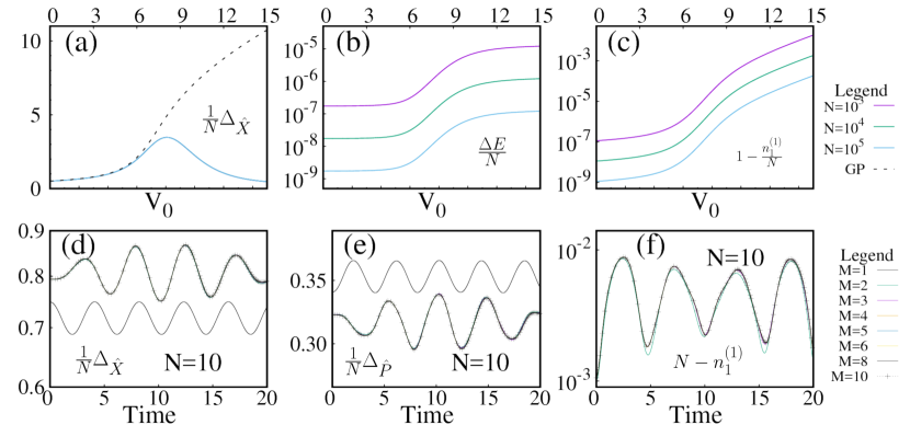
Figure 5: The position space variance, (a), of $N=10^{3},10^{4},10^{5}$ bosons with contact interactions such that $\Lambda=\lambda(t)(N-1)=0.1$ in a double well as a function of the barrier height on the many-body level (three colored/gray lines atop of each other) drastically differs from the mean-field description (black-dashed line), although the energy per particle in (b) and depletion in (c) suggest that a mean-field description is applicable (solid lines from top to bottom for $N=10^{3}$,$N=10^{4}$, and $N=10^{5}$, respectively); see also Fig. 1 of Klaiman and Alon (2015). The position variance per particle in (d), momentum variance per particle in (e), and number of depleted particles in (f) for the dynamics of $N=10$ attractive bosons in an anharmonic trap, $V(x)=0.05x^{4}$. The dynamics follow a quench of the strength of the interactions [attractive Gaussian interaction potential $\lambda(t)e^{0.5(x-x^{\prime})^{2}}$ with $\lambda(t)=-0.02$ for $t<0$ and $\lambda(t)=-0.04$ for $t\geq 0$], panels (d)–(f) replotted with data from Fig. 6 in Alon and Cederbaum (2018). A smaller distance from the exact result ($M=10$, crosses) of the lines in (d)–(f) for different orbital number $M$ indicates larger $M$ (values of $M$ in the legend): convergence with $M$ is found.

In turn, even at the IPNL the many-body wavefunction is extremely complex and very different from the mean-field one. This difference is caused by only a small amount of bosons outside the condensed mode Cederbaum (2017). Since the mean-field and many-body wavefunctions are different, the properties derived from them may also be different. This is particularly true starting from two-body properties, such as the many-particle position variance. When the variance is computed from a mean-field wavefunction it directly relates to the one-body density, because the wavefunction is built as a product of one single-particle state. When the variance, however, is computed from a many-body wavefunction it directly relates to the one-body and two-body density, i.e., it contains information about correlations in the wavefunction that is not necessarily built as a product of one single-particle state. The relation between the density of a BEC and the correlations within a BEC can therefore be probed via the variance of operators. The variance can be used as a sensitive diagnostic tool, for the excitations of BECs Theisen and Streltsov (2016); Beinke et al. (2018), for analyzing the impact of the range of interactions Haldar and Alon (2018, 2019), and for assessing convergence of numerical approaches like MCTDH-B Cosme et al. (2016); Alon and Cederbaum (2018), see Fig. 5(d)–(f) for an example convergence test with the position and momentum space variance, $\frac{1}{N}\Delta^{2}_{\hat{X}}(t)$ and $\frac{1}{N}\Delta^{2}_{\hat{p}}(t)$, respectively, in quench dynamics of attractively interacting anharmonically trapped bosons.

The many-body features of the variance of operators in a BEC depend on the strength and sign of the interaction, the geometry of the trap, and the observable under investigation, e.g., the position, momentum, or angular momentum, see Klaiman and Alon (2015); Klaiman et al. (2016); Sakmann and Schmiedmayer (2018); Alon (2019a). For bosonic systems in two-dimensional traps, additional possibilities open up for the variance. Explicitly, when computed at the many-body and mean-field levels of theory, the respective variances can exhibit different anisotropies Klaiman et al. (2018) or reflect the different effective dimensionality Alon (2019b) of the bosonic system under investigation.

IV MCTDH-F and electrons in atoms and molecules

Here, we discuss selected applications of MCTDH-F, in some cases with the incorporation of a complete active space or RAS scheme, to electron dynamics in atoms and molecules. Before discussing applications of MCTDH-F that contain a comparison with experiment in Sec. IV.2, we introduce the used observables in the following Subsection.

IV.1 Extraction of observables

Using (RAS-)MCTDH-F, photoionization cross sections have been calculated using the flux method Jäckle and Meyer (1996). The procedure, involving exterior complex scaling, has been described in detail Haxton et al. (2011) and applications were presented for beryllium and molecular hydrogen fluoride Haxton et al. (2012).

A direct method is based on expressing the observables of interest in terms of the reduced one-body density [Eq. (25) for $p=1$], for details see Madsen et al. (2018); Omiste et al. (2017). To obtain an expression for the photoelectron momentum distribution, the starting point can be the density in coordinate space. The photoelectron distribution can then be obtained by a suitable integral transformation. The density in coordinate space at position ${\bf r}$ is obtained as the expectation value $\rho(\mathbf{r};t)=\langle\Psi|\hat{\Psi}^{\dagger}(\mathbf{r})\hat{\Psi}(\mathbf{r})|\Psi\rangle$, cf. Eq. (30). In second quantization, using the orbitals [Eq. (3)] and matrix elements of the one-body density [Eq. (10)], we obtain the density [see also Eqs. (25) and (27)]:

$$\rho({\bf r};t)=\sum_{kq}\rho_{kq}\Phi_{k}^{*}({\bf r};t)\Phi_{q}({\bf r};t).$$ (36)

To obtain the photoelectron distribution, a projection on an exact scattering state, $\psi_{\bf k}(\mathbf{r})$ with momentum $\mathbf{k}$ should be performed. If this projection is restricted to a region of the simulation volume, beyond an ionization radius, where the effect of the potential from the remaining ion is small, the projection can be performed to plane waves; if the long-range Coulomb interaction is still important in that region, the projection may be done to Coulomb scattering waves Madsen et al. (2007); Omiste et al. (2017). The photoelectron momentum distribution $P$ is then given by [cf. Eq. (36)]:

$$\frac{dP}{d{\bf k}}=\sum_{kq}\rho_{kq}\tilde{\Phi}_{k}^{*}({\bf k};t)\tilde{\Phi}_{q}({\bf k};t),$$ (37)

where

$$\tilde{\Phi}_{j}({\bf k},t)=\int^{{}^{\prime}}d{\bf r}\psi_{\bf k}^{*}({\bf r})\Phi_{j}({\bf r};t),$$ (38)

and the prime on the integral sign denotes that the integral is only to be evaluated in the outer part of the simulation volume. From the momentum distribution, the energy distribution and the angular distribution can be obtained by integration. Recently, the time-dependent surface flux method Tao and Scrinzi (2012) was applied to argon and neon within a multiconfigurational framework Orimo et al. (2019). This method is also based on Eqs. (37) and (38), but requires smaller simulation volumes. The cross section can by obtained from the time-dependent calculation once the ionization probability $P_{1}$ is known Madsen et al. (2000); Foumouo et al. (2006). For example, the photoionization cross section can be extracted by Foumouo et al. (2006)

$$\sigma_{1}(\text{Mb})=1.032\times 10^{14}\omega^{2}P_{1}/(n_{p}I_{0}),$$ (39)

where $\omega$ is the angular frequency of the laser, $I_{0}$ is the peak intensity of the laser pulse in W/cm², and $n_{p}$ is the number of cycles and $P_{1}$ is the ionization probability.

Another quantity which we use below and which has received significant interest in strong-field and attosecond physics in recent years is time-delay in photoemission. This field was recently reviewed Pazourek et al. (2015). The time-delay $\tau$ can be extracted in a three-step procedure that we now discuss. (i) From the computed wavefunction, one extracts the expectation value of the radial distance $\langle r_{\vec{\xi}}(t)\rangle$ in a given direction $\vec{\xi}$ as a function of time and the linear momentum of the photoelectron $k_{\vec{\xi}}$ in that directions; it can be evaluated in different ways. For instance $\langle k_{\vec{\xi}}\rangle$, can be evaluated via integrating only in the outer part of the simulation volume Omiste et al. (2017); Omiste and Madsen (2018). (ii) Using $\langle r_{\vec{\xi}}(t)\rangle$ and $\langle k_{\vec{\xi}}\rangle$ the effective ionization time,

$$t_{\text{Coul}}=t-\frac{\langle r_{\vec{\xi}}(t)\rangle}{k_{\vec{\xi}}}=\tau_{\text{EWS}}+\Delta t_{\text{Coul}},$$ (40)

can be evaluated. Here, $\tau_{\text{EWS}}$ is the Eisenbud-Wigner-Smith (EWS) time-delay, i.e., the time-delay without the interaction with the Coulomb tail of the ion and $\Delta t_{\text{Coul}}=\frac{Z}{k_{\vec{\xi}}^{3}}\left[1-\ln(2k_{\vec{\xi}}^{2}t)\right]$ is the distortion caused by the long-ranged Coulomb potential, where $Z$ is the charge of the ion. (iii) Finally, the time-delay time is evaluated using

$$\tau=\tau_{\text{EWS}}+\tau_{\text{CLC}}.$$ (41)

Here, $\tau_{\text{EWS}}$ can be evaluated from Eq. (40) and the Coulomb-laser-coupling

$$\tau_{\text{CLC}}=\frac{Z}{k_{\vec{\xi}}^{3}}\left[2-\ln{\left(\frac{\pi k_{\vec{\xi}}^{2}}{\omega_{IR}}\right)}\right]$$

which is known, because $Z$, $k_{\vec{\xi}}$, and the frequency of the infrared pulse, $\omega_{IR}$, are known. Thus the time delay $\tau$ can readily be extracted from the solution of the (RAS-)MCTDH-F EOM Omiste and Madsen (2018).

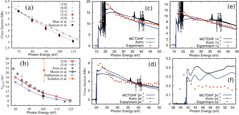
Figure 6: (a) Theoretical total photoionization cross section extracted from a calculation with a $10$-cycle linearly polarized pulse with peak intensity $10^{14}$ W/cm² as a function of the central angular frequency $\omega$ of the laser for several RAS schemes compared to the experimental data by Marr et al. Marr and West (1976) and Samson et al. Samson and Stolte (2002). (b) Relative time-delay of ionization in Ne, $\tau_{2p-2s}$, as a function of the central frequency of the XUV pulse for a $780$ nm IR pulse for $(M_{1},M_{2})=(5,\,0)$ and $(5,\,4)$ together with calculations  Feist et al. (2014); Moore et al. (2011); Dahlström et al. (2012) and the measurement Schultze et al. (2010). Total photoionization cross section (c) and its partitions in the $1\pi^{-1}$ (e), $3\sigma^{-1}$ (d), and $2\sigma^{-1}$ (f) final states. The MCTDH-F computations here used nine orbitals while the complex Kohn ones used eight. The cross sections were computed via the flux into an exterior complex scaling region Moiseyev (1998), see Haxton et al. (2012) for details. The overall agreement between MCTDH-F and experimental results Brion and Thomson (1984) is good: for all four depicted cases the salient features are reproduced for the total, $1\pi^{-1}$, and $3\sigma^{-1}$ cross sections. Reproduced with permission from  Omiste and Madsen (2018) and  Haxton et al. (2012) with copyright from APS.

IV.2 Examples involving comparison with experimental results

The processes we will focus on here are in the research area of laser-matter interactions. They are characterized by linear or perturbative interactions, where relatively few photons are exchanged with the external electromagnetic field. This reflects the current challenges with making the MCTDH-F computationally efficient in full dimension and for nonperturbative dynamics where many photons are exchanged. For validation of the MCTDH-F methodology, comparisons with experiments have focused on calculating photoabsorption cross sections Haxton et al. (2012); Omiste and Madsen (2018, 2019), where accurate experimental data are available. In addition, XUV transient absorption spectra Liao et al. (2017) and time delays in photoionization dynamics Omiste et al. (2017); Omiste and Madsen (2018) have been considered. Here, we consider cross section and time-delay studies as illustrative examples.

IV.2.1 Photoionization cross sections

In the case of photoionization, Fig. 6(a) shows a comparison for atomic neon between the predictions of theory at different levels of approximation and experimental cross section data.

The values of the theoretical cross sections in Fig. 6(a) are obtained by the procedure described in Sec. IV.1. From the agreement between theory and experiment in Fig. 6(a), it can be concluded that it is possible to obtain a precise prediction of the photoionization cross section using an explicitly time-dependent method, the RAS-MCTDH-F, using the procedure discussed in relation to Eq. (39). A second key point to be noticed from Fig. 6(a) is related to the choice of the ${\cal P}_{1}$ and $\mathcal{P}_{2}$ subspaces and the number orbitals in them. We consider here the RAS-MCTDH-F-D method, cf. Fig. 2 for an illustration of the ${\cal P}_{1}$ and $\mathcal{P}_{2}$ spaces. The ’D’ in the acronym of the method denotes “doubles”: only double excitations from the $\mathcal{P}_{1}$ to the $\mathcal{P}_{2}$ spaces are allowed. In this example there is no space $\mathcal{P}_{0}$ with always occupied orbitals like the one used to construct “complete active space” methods Sato and Ishikawa (2013). Such a choice of active space and excitation scheme reduces the number of configurations compared with the MCTDH-F method with no restrictions, and as is seen from Fig. 6(a), can still yield accurate results: convergence is obtained by increasing the number of orbitals in $\mathcal{P}_{2}$ from $M_{2}=0$ to $M_{2}=9$. In this manner the accuracy of different approximations from the mean-field time-dependent Hartree-Fock (TDHF) to approaches including more correlation is systematically explored.

Comparisons between theory and experiment for photoionization cross sections have also been performed for atomic beryllium and the hydrogen fluoride molecule Haxton et al. (2012). In these latter cases, full MCTDH-F is considered. Similar to the RAS-MCTDH-F example above, convergence of the MCTDH-F results for the cross sections were obtained with increasing number of active orbitals. We highlight here the good agreement of the photoionization cross sections obtained for hydrogen fluoride molecules with the experimental Brion and Thomson (1984) and complex Kohn theoretical Schneider and Rescigno (1988); Rescigno and Orel (1991) results, see Fig. 6(c)–(f).

IV.2.2 Time delay in photoionization

RAS-MCTDH-F, has been applied to the time-delay in photoionization in neon Omiste and Madsen (2018), where experimental data is available Schultze et al. (2010); Isinger et al. (2017). It is the advent of new light sources for ultrashort light pulses with durations down to the attosecond timescale that has allowed addressing questions like time delay in photoionization in experiments. In Fig. 6(b), the time delay in photoionization between the $2s$ and the $2p$ electrons in neon is shown in units of attoseconds ($1$ as = $10^{-18}$s). A collection of theoretical results and a measurement point  Schultze et al. (2010) are presented in Fig. 6(b) as a function of photon energy $\omega$ (in atomic units, $\hbar=1$, and for convenience the values in atomic units have been converted to eV, $1$ a.u. = $27.21$ eV).

The positive value of the time delay can be interpreted as if it takes longer time for the $2p$ than for the $2s$ orbital to ionize. Such an interpretation in terms of orbitals, however, assumes a mean-field picture. Theory and experiment have addressed the question about relative time delay between ionization into the two channels

$$\text{Ne}~{}[(1s^{2}2s^{2}2p^{6}){}^{1}\text{S}^{e}] \rightarrow \text{Ne}^{+}~{}[(1s^{2}2s^{2}2p^{5}){}^{2}\text{P}^{o}]+e^{-}(s,d)$$

$$\text{Ne}~{}[(1s^{2}2s^{2}2p^{6}){}^{1}\text{S}^{e}] \rightarrow \text{Ne}^{+}~{}[(1s^{2}2s2p^{6}){}^{2}\text{S}^{e}]+e^{-}(p),$$

where the dominant configurations have been used to denote the ground state in the neutral as well as the ground and excited state in the ion. Note that dipole selection rules dictate the possible values of the angular momenta in the final channels. From Fig. 6(b), it is seen that all the theories predict a decreasing time delay as a function of the photon energy in the considered energy range. All theoretical values are also smaller than the experimental result. Recently, measurements with an interferometric technique Isinger et al. (2017) reported a lower value of the time delay in better agreement with the theory results. In the following, we focus on the RAS-MCTDH-F results with $(M_{1},M_{2})$ at $(5,0)$ and at $(5,4)$, see Fig. 6(b). For neon, the $(5,0)$ results correspond to the TDHF case, i.e., one active orbital for each pair of electrons. The $(5,4)$ case includes more correlations and has $5$ orbitals in $\mathcal{P}_{1}$ and $4$ orbitals in $\mathcal{P}_{2}$. The transitions between $\mathcal{P}_{1}$ and $\mathcal{P}_{2}$ occur by double excitation only. As seen from Fig. 6(b), part of the overall trend of the time delay can be described at the TDHF-level of theory.

Note that there are other cases of interest, where the ionization step can not be captured by TDHF. For example in beryllium, photoionization of the ground state into the channel Be${}^{+}[(1s^{2}2p)^{2}\text{P}^{o}]+e^{-}(s\text{ or }d)$ changes two orbitals in the dominant configurations by the action of the one-body photoionization operator. Therefore, that process can not be described by TDHF Omiste et al. (2017).

V Applications, theoretical, and numerical development

We now discuss theoretical and numerical developments within and beyond (RAS-)MCTDH-X.

V.1 MCTDH-X-based development

V.1.1 Numerical methods

Since the introduction of MCTDH-F Zanghellini et al. (2003); Kato and Kono (2004); Caillat et al. (2005) and MCTDH-B Streltsov et al. (2007); Alon et al. (2007c); Alon et al. (2008) many numerical techniques and theory extensions were developed that extend the applicability of MCTDH-X.

For long-ranged interparticle interactions where the interaction potential is a function of the distance of the particles, $W(\mathbf{r}_{i},\mathbf{r}_{j};t)=W(\mathbf{r}_{i}-\mathbf{r}_{j};t)$, the so-called interaction matrix evaluation via successive transforms (IMEST) has been developed Sakmann (2011). IMEST rewrites the local interaction potentials as a collocation using fast Fourier transforms. IMEST has been applied for solving the TDSE with MCTDH-X, for (time-dependent) harmonic interparticle interactions Lode et al. (2012a); Lode (2015); Fasshauer and Lode (2016), dipolar interactions Chatterjee and Lode (2018); Chatterjee et al. (2019a, b), and general long-range interaction potentials Streltsov (2013); Streltsova et al. (2014); Fischer et al. (2015); Haldar and Alon (2018) and screened Coulomb interactions Fasshauer and Lode (2016).

The development of an implementation of MCTDH-F using a multiresolution Cartesian grid Sawada et al. (2016) holds promise to provide improved adaptive representations for the dynamics of the wavefunction of electrons in atoms and molecules. Moreover, we note the implementation of the infinite-range exterior complex scaling method Orimo et al. (2018) and the introduction of a space partitioning concept Miyagi and Madsen (2017) in combination with RAS-MCTDH-F. We mention that it has been shown that the inclusion of complex absorbing potentials to describe situations like ionization where particles are leaving the region of interest requires one to use a Master equation of Lindblad form for the time-evolution of the density matrix, see Selstø and Kvaal (2010). To solve this Master equation, $\rho$-MCTDH-F has been formulated in Kvaal (2011).

The efficient evaluation of the Coulomb interaction integrals [Eq. (16) with $\hat{W}$ being the Coulomb interaction] is instrumental to study real-world dynamics of electrons in atoms and molecules in three spatial dimensions. We mention here a $sinc$-DVR approach that enables an efficient collocation, i.e., Fast-Fourier-transform-based evaluation of the Coulomb interactions in by exploiting the triple-Toeplitz structure of the kinetic energy operator Jones et al. (2016).

We note the recent successful implementation and application of the adaptive removal and addition of configurations, so-called dynamical pruning Larsson and Tannor (2017); Wodraszka and Carrington (2017) for dynamics computed with MCTDH-B Köhler et al. (2019).

V.1.2 Theoretical progress

The MCTDH-X methodology has also been used to obtain descriptions of the dynamics generated by Hubbard Hamiltonians. In Lode and Bruder (2016), the operators that create or annihilate particles in the time-independent first-band Wannier basis functions of the Hubbard lattice are expressed as effective, creation or annihilation operators for particles in a time-dependent superposition of all lattice sites. The resulting EOM are identical to the MCTDH-X EOM [Eqs. (8),(13)], albeit with a special representation of the kinetic and potential energy. In  Sakmann et al. (2011), generalized time-dependent Wannier functions which are a superposition of many bands are proposed, to increase the accuracy of the representation of the many-boson wavefunction beyond the single-band Hubbard model. In  Grond et al. (2013); Alon et al. (2014), a linear-response framework for the EOM of MCTDH-X, the so-called LR-MCTDH-X, is put forward that allows to obtain highly accurate information about the excitation spectrum of the considered many-body Hamiltonian, as benchmarked in Beinke et al. (2017, 2018). Recently, the Fourier transform of the auto-correlation function was used to obtain the spectrum for a bosonic many-body system Lévêque and Madsen (2019).

For the dynamics of electrons in molecules, an approach termed “multi-configuration electron-nuclear dynamics method” (MCEND) was developed Nest (2009) and applied to lithium hydride Ulusoy and Nest (2012). This MCEND method represents the total molecular wavefunction as a direct (tensor) product of an MCTDH-type wavefunction for the nuclei with an MCTDH-F-type wavefunction of the electrons. Other approaches to deal with coupled electronic and nuclear dynamics have been developed and applied for diatomics Haxton et al. (2011, 2015); Kato and Yamanouchi (2009); Lötstedt et al. (2019b).

Recent developments of the so-called extended-MCTDH-F in  Kato and Yamanouchi (2009) consider coupled electron-nuclear dynamics and molecular wavefunctions and include extensive investigations on molecular hydrogen Kato et al. (2015); Ide et al. (2014) and cationic molecular hydrogen in intense laser fields Lötstedt et al. (2019b, a) as well as a strategy to efficiently partition the configuration space of MCTDH-F Lötstedt et al. (2016).

The multiple active space model put forward in  Sato and Ishikawa (2015) introduces a flexible and possibly adaptive approach to construct representations for the $N$-body Hilbert space with multiconfigurational methods.

We mention here the development, application, and successful benchmark against MCTDH-F predictions for high-harmonic generation of a method that time-evolves the two-body density matrix [cf. Eq. (25) for $p=2$] without resorting to a wavefunction at all Lackner et al. (2015, 2017). These methods for the two-body density matrix offer a similar accuracy to MCTDHF approaches while being much less computationally demanding.

The unfavorable scaling of the number of coefficients in the MCTDH-X ansatz with the number of orbitals impedes the application of MCTDH-X to systems with many electrons or many bosons with more than a few orbitals. Truncation strategies for the coefficient vector include the RAS approach from quantum chemistry Olsen et al. (1988) that results in RAS-MCTDH-F Miyagi and Madsen (2013, 2014) and RAS-MCTDH-B Lévêque and Madsen (2017, 2018) theories including a special consideration of single-particle excitations Miyagi and Bojer Madsen (2014). The “complete active space” (CAS) truncation approach to limit the number of coefficients was also investigated, see Sato and Ishikawa (2013) and, including a generalization to several active spaces Sato and Ishikawa (2015). For an MCTDH-F formulation for completely general configuration spaces where different variational principles become inequivalent, see  Haxton and McCurdy (2015).

For a review of time-dependent multiconfigurational theories for electronic and nuclear motion in molecules in intense fields see Kato et al. (2018), for an overview of RAS-MCTDH-X theory see Madsen et al. (2018).

V.2 MCTDH-B applications

The archetypical example for the emergence of fragmentation in systems of interacting bosons is the double well potential Spekkens and Sipe (1999). Using MCTDH-B for bosons in double-well traps, the reduced density matrices and Glauber correlation functions Sakmann et al. (2008), the dynamical emergence Streltsov et al. (2007); Sakmann et al. (2009, 2010); Sakmann (2011) and the universality Sakmann et al. (2014) of fragmentation have been investigated. It is worthwhile to highlight that the works Sakmann et al. (2009, 2010) report converged solutions of the TDSE and demonstrate that the commonly applied Bose-Hubbard model may fail to describe the many-body states for parameter regimes where it was deemed to yield a good approximation to the many-body state. We note that the excitation spectra of interacting bosons in double wells Grond et al. (2013); Theisen and Streltsov (2016), in lattices Beinke et al. (2017), and under rotation Beinke et al. (2018) have been investigated with LR-MCTDH-B. Recent work with MCTDH-B explores the connection between quantum fluctuations, correlations, and fragmentation Nguyen et al. (2019); Marchukov and Fischer (2019).

Solitons in BEC are thought to be coherent and condensed; several investigations with MCTDH-B Streltsov et al. (2008, 2011); Cosme et al. (2016), however, have shown that fragmentation and correlations do emerge in their dynamics.

Vortices in ultracold bosonic atoms are conventionally modelled by mean-field approaches Gross (1961); Pitaevskii (1961). Applications of MCTDH-B to interacting bosonic atoms have, however, demonstrated that correlations and fragmentation may emerge as soon as the many-body state contains significant angular momentum Tsatsos and Lode (2015); Beinke et al. (2015); Weiner et al. (2017). This emergence of correlations and fragmentation marks the breakdown of the mean-field description and is anticipated from pronounced many-body effects in the excitation spectra of bosonic systems with angular momentum as obtained from LR-MCTDH-B Beinke et al. (2018).

BECs in high-finesse optical cavities have been used as a quantum simulator for the Dicke model Brennecke et al. (2007); Baumann et al. (2010). Using MCTDH-B it was shown that the phase diagram of the cold-atom system in the cavity is richer than the phase diagram of the Dicke model and thus the mapping to the Dicke model may break down Lode and Bruder (2017); Lode et al. (2018); Lin et al. (2019).

V.3 MCTDH-F applications

The MCTDH-F was first applied to strong-field ionization of one-dimensional (1D) model molecules with up to eight electrons Zanghellini et al. (2003), harmonic quantum dots, a 1D model of helium Zanghellini et al. (2004), and a 1D jellium model Nest (2006). Total ionization spectra in strong laser fields were reported for 1D systems with up to six active electrons and strong correlation effects were reported in the shape of photoelectron peaks and the dependence of ionization on molecule size Caillat et al. (2005). Later, the effect of the reduction in dimensionality from three to one dimension was discussed Jordan et al. (2006). In the strong-field regime, multielectron and polarization effects have been considered in connection with application to high-order harmonic generation at fixed internuclear distance in model systems Jordan and Scrinzi (2008); Sukiasyan et al. (2009, 2010); Miyagi and Madsen (2013, 2014), in carbon monoxide Ohmura et al. (2018) as well as helium, beryllium, and neon Sawada et al. (2016).

In molecules, MCTDH-F was applied to H₂ at fixed internuclear distance Kato and Kono (2004, 2008). The MCTDH-F results reported for molecules include calculations of vertical excitation energies, transition dipole moments, and oscillator strengths for lithium hydride and methane Nest et al. (2007), as well as considerations of the response of lithium hydride to few-cycle intense pump fields followed by a probe pulse Nest et al. (2008). Work on characterizing multielectron dynamics by considering energies and amplitudes was reported Ohmura et al. (2014). The inclusion of nuclear motion has also been considered Nest (2009); Kato and Yamanouchi (2009); Haxton et al. (2011); Anzaki et al. (2017).

Concerning few-photon processes, MCTDH-F has been applied to the simulation of the two-photon ionization of helium including a comparison with the time-dependent configuration interaction method Hochstuhl and Bonitz (2011). The population transfer between two valence states of the lithium atom with a Raman process via intermediate autoionizing states well above the ionization threshold was investigated Li et al. (2014). A two-color core-hole stimulated Raman process was studied in nitric oxide Haxton and McCurdy (2014) and Raman excitations of atoms through continuum levels were considered for neon Greenman et al. (2017). Moreover, a procedure was suggested for using transient absorption spectroscopy above the ionization threshold to measure the polarization of the continuum induced by an intense optical pulse Li et al. (2016). Recently, a comparison of MCTDH-F and experimental results was reported in a study using XUV transient absorption spectroscopy to study autoionizing Rydberg states of oxygen Liao et al. (2017). RAS-MCTDH-F was applied to study electron correlation and time delay in beryllium Omiste et al. (2017), neon  Omiste and Madsen (2018), and effects of performing calculations with or without a filled core space Omiste and Madsen (2019).

V.4 Multilayer and second-quantized-representation approaches

Multilayer approaches Wang and Thoss (2003); Manthe (2008) provide a powerful and promising generalization of the standard MCTDH. In the multilayer (ML) strategy, the MCTDH is applied recursively Manthe (2008); Vendrell and Meyer (2011): first, the wavefunction is represented as a sum of products of “single-particle” functions (first layer); second, the “single-particle” functions of the first layer are again represented by an MCTDH-type wavefunction, i.e., a sum of products of (second-layer) “single-particle” functions, and so on. Here, we have used quotation marks on the term single-particle, because several degrees of freedom may be combined into multi-mode single-particle functions using mode combination Worth et al. (1998, 1999); Raab and Meyer (2000), i.e., a single-particle function may still be a high-dimensional function. In the bottom or last layer, the single-particle functions are then expanded on a primitive time-independent basis.

We mention here a fundamental relation between density matrix renormalization group and matrix-product-state methods reviewed in Schollwöck (2005, 2011) and ML-MCTDH: mathematically, both methods fall into the class of so-called hierarchical low-rank tensor approximations, a concept which has, for instance, enabled progress in devising new efficient time-integration schemes Lubich et al. (2018); Falcó et al. (2019) that are also applicable for (RAS-)MCTDH-X.

The multilayer approach requires a configuration space of distinguishable degrees of freedom as in MCTDH; the multilayer approach can thus not be directly combined with the MCTDH-X, since the latter restricts the configuration space to include only configurations of a fixed number of strictly indistinguishable particles that have the correct fermionic or bosonic symmetry.

In the following, we introduce two distinct multilayer approaches for indistinguishable particles, namely the ML-MCTDH in second quantized representation (ML-MCTDH-SQR) and the ML-MCTDH-X. ML-MCTDH-X and ML-MCTDH-SQR are not affected by the previous incompatibility of the MCTDH-X approach and multilayering. The ML-MCTDH-X approach uses a multilayer formalism for Cartesian coordinates or different species of indistinguishable particles and ML-MCTDH-SQR uses the occupation numbers of the orbitals as distinguishable degrees of freedom for an MCTDH-type wavefunction where multilayering can be applied.

V.4.1 ML-MCTDH in second quantized representation

We begin by noting that the SQR approach is actually independent of the ML approach. However, historically, SQR was introduced on top of ML-MCTDH; the resulting ML-MCTDH-SQR was put forward in  Wang and Thoss (2009) and reviewed in  Wang (2015); Manthe (2017). Below, we therefore discuss the two ingredients together.

The SQR approach is based on the fact that the second-quantized configurations $|\vec{n}\rangle=|n_{1},n_{2},...,n_{M}\rangle$ in Eq. (2) can formally be written as a Hartree product [see Chapters 1 and 3 in Röpke (1999)]:

$$|n_{1},n_{2},...,n_{M}\rangle\equiv|n_{1}\rangle|n_{2}\rangle\cdots|n_{M}\rangle.$$ (43)

Thus, the occupation numbers $n_{1},n_{2},...,n_{M}$ of the time-independent orbitals are used as the degrees of freedom in an ML-MCTDH-type wavefunction to obtain the ansatz of the ML-MCTDH-SQR approach.

Just like ML-MCTDH, the ML-MCTDH-SQR representation features a configurational expansion of distinguishable degrees of freedom; however, these degrees of freedom are – unlike for standard ML-MCTDH – represented in a second quantized notation tied to a time-independent basis. As Eq. (43) clearly demonstrates, the ML-MCTDH-SQR breaks apart the configurations $|n_{1},...,n_{M}\rangle$, whereas the (ML-)MCTDH-X approaches deals with them as unbreakable entities. ML-MCTDH-SQR therefore, via employing a different approach to the representation of Fock space, uses multilayering in the very same way as the original ML-MCTDH, but now for indistinguishable particles. In other words, ML-MCTDH-SQR thus enables the use of deeply multi-layered wavefunction representations which is incompatible with the particle-number based configuration selection of the MCTDH-X approaches. We note, that the reformulation of a configuration as a Hartree product in Eq. (43) requires that, for the case of indistinguishable fermions, the initially chosen order of the terms in the product has to be tracked and maintained at all times Wang and Thoss (2009); Wang (2015).

The ML-MCTDH-SQR theory has, for instance, been successfully applied to the dynamics of vibrationally-coupled electron transport in a model molecular junction Wang and Thoss (2009, 2016) and transport in the Anderson impurity model Wang and Thoss (2018). Recently, ML-MCTDH-SQR has been generalized to allow for variationally time-dependent optimized second-quantized (oSQR) degrees of freedom yielding the ML-MCTDH-oSQR approach Manthe and Weike (2017). Most recently, strategies to incorporate particle conservation in ML-MCTDH-oSQR were discussed in  Weike and Manthe (2020).

V.4.2 ML-MCTDH-X

The ML-MCTDH-X approach uses an MCTDH-type representation for the distinguihsbale degrees of freedom in systems of identical particles. These distinguishable degrees of freedom can be the species in a mixture of identical particles, the differernt Cartesian coordinates of an orbital in more than one spatial dimension, and/or its spin. The indistinguishable parts of the wavefunction in ML-MCTDH-X are, themselves, represented by MCTDH-X-type expansions Cao et al. (2013); Krönke et al. (2013); Cao et al. (2017). In other words, in ML-MCTDH-X the statistics of indistinguishable particles is maintained via an MCTDH-X-type wavefunction. We note, that an MCTDH-X formulation for mixtures of identical particles without multilayering exists Alon et al. (2007a). The ML-MCTDH-X approach has been applied successfully to mixtures of ultracold bosons and fermions Mistakidis et al. (2018); Erdmann et al. (2018); Siegl et al. (2018) and bosons in more than one spatial dimension Bolsinger et al. (2017b, a).

V.5 Orbital-adaptive time-dependent coupled cluster

To reduce the numerical effort in solving the TDSE to become polynomial, the so-called coupled cluster method (CC) Coester and Kümmel (1960); Čížek (1966, 2007); Čižek and Paldus (1971) can be employed. Although CC uses a different type of ansatz than MCTDH-X, we mention it here, because recent developments include approaches with a time-dependent, variationally optimized basis and are thus related to MCTDH-X and RAS-MCTDH-X.

The conventional (time-dependent) CC uses time-dependent excitation amplitudes, but does not use a set of time-dependent orbitals in the representation of the wavefunction. The standard CC’s ansatz can be generalized to include time-dependent amplitudes and orbitals. This generalization of the ansatz in combination with a generalized, so-called bivariational principle, leads to the equations-of-motion of the orbital-adapted time-dependent coupled cluster theory Kvaal (2012, 2013); Pedersen and Kvaal (2019). We identify the application of the bivariational principle for the derivation of the MCTDH-X EOM for ansatzes with restricted configuration spaces [like in Eq. (17)] as an open question.

When a real-valued variational principle is used, the fully time-dependent coupled cluster ansatz yields the EOM of the time-dependent optimized CC Sato et al. (2018a, b). The latter theory allows the self-consistent computation of eigenstates via imaginary time propagation and has been applied to single- and double ionization as well as high-harmonic-generation in argon Sato et al. (2018a).

VI Conclusions and Frontiers

In this Colloquium, we introduced the MCTDH-B and the MCTDH-F methods for full and for restricted configuration spaces. We highlighted the use and versatility of MCTDH-X with benchmarks against exactly solvable models as well as direct comparisons with experimental applications.

The development of methods for the time-dependent many-body Schrödinger equation in the field of MCTDH-X and beyond, that we have portrayed in our present Colloquium, has yielded highly efficient and flexible numerical approaches. This flexibility, however, comes with an increasing number of parameters to tune the performance and accuracy of the given approach – we name here as examples the tree structure in multilayering approaches Wang and Thoss (2009); Wang (2015); Manthe (2015); Manthe and Weike (2017), and the partitioning of Hilbert space into multiple occupation-restricted active spaces Sato and Ishikawa (2015) or into or $\mathcal{P}_{1}$ and $\mathcal{P}_{2}$ (Fig. 2) in the RAS-MCTDH-X approach Miyagi and Madsen (2013, 2014); Lévêque and Madsen (2017, 2018). We thus observe that the recent methodological developments demand an ever larger and more complicated set of parameters to be configured by their users.

Such a development towards higher complexity in the application of methods is not desirable, because it makes applications ever more tedious. The trend towards more complexity could possibly be overcome by introducing additional adaptivity. We mention here the recent fascinating developments with adaptive tensor representations Grasedyck et al. (2013); Ballani and Grasedyck (2014), an adaptive number of configurations Wodraszka and Carrington (2017); Larsson and Tannor (2017); Haxton and McCurdy (2015); Miyagi and Madsen (2013, 2014); Lévêque and Madsen (2017); Köhler et al. (2019), an adaptive number of single-particle functions Lee and Fischer (2014); Mendive-Tapia et al. (2017), optimally chosen unoccupied orbitals Manthe (2015), adaptive grids Sawada et al. (2016), and an adaptive construction of the many-particle Hilbert space Sato and Ishikawa (2015). We thus envision a flexible theory and implementation that combines multiple of the above multiconfigurational methods in an adaptive framework to solve the many-particle Schrödinger equation: according to a simple/single input – for instance an error threshold – the Hilbert space is automatically and adaptively partitioned and represented while for each of the partitions of it (an adaptive version of) the best-suited multiconfigurational methods is used.

Interestingly, the extended-MCTDH-F and multi-configuration electron-nuclear dynamics method (MCEND) ansatzes, proposed in  Kato and Yamanouchi (2009) and  Nest (2009), respectively, represent the total wavefunction as a (tensor) product of wavefunctions of different species of particles. In the case of extended-MCTDH-F, the wavefunction is a product of two MCTDH-F-type wavefunctions and in the case of MCEND, the wavefunction is a product of an MCTDH-F-type wavefunction with an MCTDH-type wavefunction for distinguishable particles. Such a multi-species wavefunction – as well as bulk of the multiconfigurational methods developed for restricted, multiple, and general active spaces – is amenable to multilayer approaches. The combination of truncation methods for the configuration space, including the dynamical pruning approaches Larsson and Tannor (2017); Wodraszka and Carrington (2017); Köhler et al. (2019), with ML-MCTDH-X or ML-MCTDH-(o)SQR is one of the frontiers that we see in the further development with multiconfigurational approaches.