Finite type $\xi$-asymptotic lines of plane fields in $\mathbb{R}^{3}$

Abstract.

We prove that a finite type curve is an $\xi$-asymptotic line (without parabolic points) of a suitable plane field. It is also given an explicit example of a hyperbolic closed finite type $\xi$-asymptotic line. These results obtained here are generalizations, for plane fields, of the results of V. Arnold [4, Theorems 2, 3 and 5]. Keywords: closed asymptotic lines, plane field, parabolic points.

MSC(2000): 53C12, 37C27, 34C25.

1. Introduction

A regular plane field in $\mathbb{R}^{3}$ is usually defined by the kernel of a differential form or an unitary vector field $\xi\colon\mathbb{R}^{3}\to\mathbb{R}^{3}$. In this last case $\xi(p)$ is the normal vector to the plane at point $p$. The classical and germinal work about plane fields in $\mathbb{R}^{3}$ is [14].

The normal curvature of a plane field is defined by (see [2] and [5])

$$k_{n}(p,dr)=-\frac{\langle d\xi(p),dr\rangle}{\langle dr,dr\rangle}.$$ (1.1)

For integrable plane fields the normal curvature is the usual concept of curves on surfaces.

The regular curves $\gamma\colon I\to\mathbb{R}^{3}$ such that $k_{n}(\gamma(t),\gamma^{\prime}(t))=0$ are called $\xi$-asymptotic lines and the directions $dr$ such $k_{n}(p,dr)=0$ are called $\xi$-asymptotic directions.

Recall that asymptotic lines on surfaces are regular curves $\gamma$ such that $k_{n}(\gamma(t),\gamma^{\prime}(t))=0$. Also, asymptotic lines are the curves $\gamma$ such that the osculating plane of $\gamma$ coincides with the tangent plane of the surface along it, so asymptotic lines are of extrinsic nature.

The local study, and singular aspects of asymptotic lines on surfaces in $\mathbb{R}^{3}$, near parabolic points, is a very classical subject, see [6, 7, 8], [9] and references therein.

The study of closed asymptotic lines of surfaces in $\mathbb{R}^{3}$ under the viewpoint of qualitative theory of differential equations is more recent, see [6, 7, 8]. It is worth to mention that existence of closed asymptotic lines on the tubes of “T-surfaces”  is still an open problem. See [1, page 107] and [11].

Also, it is not known if there is a surface in $\mathbb{R}^{3}$ having a cylinder region foliated by closed asymptotic lines (see [13, page 110]). In $\mathbb{S}^{3}$ all asymptotic lines of the Clifford torus are globally defined and they are the Villarceau circles.

V. Arnold in [4] studied the topology of asymptotic lines being curves of type $(t,t^{m},t^{n})$ near $t=0$, which are called of finite type. Also it was shown in [4] that the projection of a closed asymptotic line of an hyperbolic surface of graph type $(x,y,h(x,y))$ in the horizontal plane $(x,y)$ cannot be a starlike curve.

The main results of this work are the following.

The Theorem 3.1 states that any finite type curve is an $\xi$-asymptotic line of a suitable plane field in $\mathbb{R}^{3}$.

The Theorem 4.3 gives an example of a hyperbolic closed finite type $\xi$-asymptotic line of a plane field in $\mathbb{R}^{3}$.

2. Preliminaries and Previous Results

In this paper, the space $\mathbb{R}^{3}$ is endowed with the Euclidean norm $|\cdot|=\langle\cdot,\cdot\rangle^{\frac{1}{2}}$.

Definition 2.1 ([10, Definition 5.15]).

A subset $\Omega\subset\mathbb{R}^{2}$ is called a starlike convex set if there is a point $p\in\Omega$, called the star point, such that, for every $q\in\Omega$, the segment $\overline{pq}$ lies in $\Omega$. The boundary of a starlike convex set is called a starlike curve.

Theorem 2.2 (D. Panov, see [4]).

The projection of a closed asymptotic line of a surface $z=\varphi(x,y)$ to the plane $\{z=0\}$ cannot be a starlike curve (in particular, this projection cannot be a convex curve).

Definition 2.3 ([4]).

A smoothly immersed curve $\gamma:I\to\mathbb{R}^{3}$ is said to be of finite type at a point $x$, if $\{\gamma^{\prime}(x),\gamma^{\prime\prime}(x),\ldots,\gamma^{(k)}(x)\}$ generate all the tangent space $T_{\gamma(x)}\mathbb{R}^{3}$ for some $k\in\mathbb{N}.$ Here $\gamma^{(k)}(x)$ denotes the derivative of order $k$ of $\gamma$. In a neighborhood of this point, the curve is parametrized locally by $\gamma(x)=(x,a_{m}x^{m}+\mathcal{O}^{m+1}(x),b_{n}x^{n}+\mathcal{O}^{n+1}(x))$, where $m,n\in\mathbb{N}$, $a_{m}b_{n}\neq 0$ and $1<m<n$.

The set $\{1,m,n\}$, $(1<m<n)$, of the degrees of $\gamma$ is called the symbol of the point. If $n=m+1$, then $\gamma$ is said to be of rotating type at the point.

If a curve is of finite type (resp. rotating type) at every point, then it is called of finite type curve (resp. rotating type curve).

A finite type curve $\gamma$ can be have inflection points, i.e., points where the curvature of $\gamma$ vanishes.

Arnold’s Theorem (See [4]).

An asymptotic curve of finite type on a hyperbolic surface is a rotating curve.

Every rotating space curve of finite type is an asymptotic line on a suitable hyperbolic surface.

A new proof of Arnold’s Theorem will be given in Appendix Finite type $\xi$-asymptotic lines of plane fields in $\mathbb{R}^{3}$.

2.1. Plane fields in $\mathbb{R}^{3}$

Let $\xi:\mathbb{R}^{3}\rightarrow\mathbb{R}^{3}$ be a vector field of class $C^{k}$, where $k\geq 3$.

Definition 2.4.

A plane field $\xi$ in $\mathbb{R}^{3}$, orthogonal to the vector field $\xi$, is defined by the 1-form $\langle\xi,dr\rangle=0$, where $dr$ is a direction in $\mathbb{R}^{3}$. See Fig. 1.

Theorem 2.5 ([2, Jacobi Theorem, p.2]).

There exists a family of surfaces orthogonal to $\xi$ if, and only if, $\langle\xi,curl(\xi)\rangle\equiv 0$.

A plane field $\xi$ is said to be completely integrable if $\langle\xi,curl(\xi)\rangle\equiv 0$. A surface of the family of surfaces orthogonal to $\xi$ is called an integral surface.

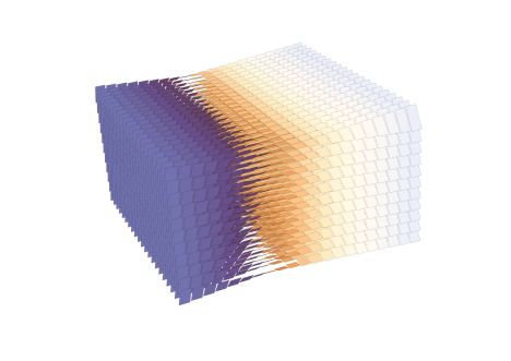
Figure 1. Plane field $\xi$ in $\mathbb{R}^{3}$ defined by the 1-form $dz-ydx=0$. The vector field $\xi$ is given by $\xi(x,y,z)=(-y,0,1)$.

2.2. Normal curvature of a plane field

Definition 2.6 ([2, p. 8]).

The normal curvature $k_{n}$ of a plane field in the direction $dr$ orthogonal to $\xi$ is defined by

$$k_{n}=\frac{\langle d^{2}r,\xi\rangle}{\langle dr,dr\rangle}=-\frac{\langle dr,d\xi\rangle}{\langle dr,dr\rangle}.$$ (2.1)

This definition agrees with the classical one given by L. Euler, see [5].

In the plane $\pi(p_{0},dr)$ generated by $\xi(p_{0})$ and $dr$ (direction orthogonal to $\xi(p_{0})$) we have a line field $\ell(p)$ orthogonal to vector $\bar{\xi}(p)\in\pi(p_{0},dr)$ obtained projecting $\xi(p)$ in the plane $\pi(p_{0},dr)$, with $p\in\pi(p_{0},dr)$. The integral curves $\varphi_{p}(t)$ of the line field $\ell$ are regular curves and $k_{n}(p_{0},dr)$ is the plane curvature of $\varphi_{p_{0}}(t)$ at $t=0$. See Fig. 2.

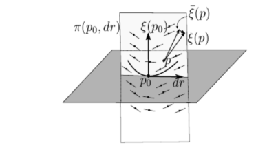
Figure 2. Line field and normal curvature $k_{n}(p_{0},dr)$.

2.3. $\xi$-asymptotic lines and parabolic points of a plane field

The $\xi$-asymptotic directions of a plane field $\xi$ are defined by the following implicit differential equation

$$\begin{split}\langle\xi,dr\rangle=0,\ \ \langle d\xi,dr\rangle=0.\end{split}$$ (2.2)

and will referred as the implicit differential equation of the $\xi$-asymptotic lines.

A solution $dr$ of equation (2.2) is called an $\xi$-asymptotic direction. A curve $\gamma$ in $\mathbb{R}^{3}$ is an $\xi$-asymptotic line if $\gamma$ is an integral curve of equation (2.2). Analogously to the case of asymptotic lines on surfaces, for plane fields the osculating plane of an $\xi-$asymptotic line coincides with the plane of the distribution of planes passing through the point of the curve. See also [3, page 29].

Definition 2.7.

If at a point $r$ there exists two real distinct $\xi$-asymptotic directions (resp. two complex $\xi$-asymptotic directions), then $r$ is called a hyperbolic point (resp. elliptic point).

Definition 2.8.

If at $r$ the two $\xi$-asymptotic directions coincide or all the directions are $\xi$-asymptotic directions then $r$ is called a parabolic point.

Example 2.9.

The circle in $\mathbb{R}^{3}$ given by $x^{2}+y^{2}=1$, $z=0$, is an $\xi$-asymptotic line without parabolic points of the plane field $\xi$ defined by the orthogonal vector field $\xi=(\rho,\varrho,\sigma)$, where $\rho=x^{2}yz+y^{3}z-x^{2}y-y^{3}+xz-2yz+y$, $\varrho=x^{3}-x^{3}z-xy^{2}z+xy^{2}+2xz+yz-x$ and $\sigma=-x^{2}-y^{2}$. The plane field $\xi$ is not completely integrable. By the Theorem 2.2, this circle cannot be an asymptotic line of a regular surface $z=\varphi(x,y)$.

Proposition 2.10.

Given a plane field $\xi$, let $\varphi:\mathbb{R}^{3}\rightarrow\mathbb{R}$ be a differentiable nonvanishing function. Then a curve $\gamma$ is an $\xi$-asymptotic line if, and only if, $\gamma$ is an $\xi$-asymptotic line of the plane field $\widetilde{\xi}$ orthogonal to the vector field $\widetilde{\xi}=\varphi\xi$.

Proof.

The implicit differential equation of $\xi$-asymptotic lines of $\widetilde{\xi}$ is given by

$$\langle\widetilde{\xi},dr\rangle=\varphi\langle\xi,dr\rangle=0,\ \ \langle d\widetilde{\xi}(dr),dr\rangle=d\varphi(dr)\langle\xi,dr\rangle+\varphi\langle d\xi(dr),dr\rangle=0.$$ (2.3)

Then $\gamma$ is an $\xi$-asymptotic line of $\xi$ if, and only if, $\gamma$ is an $\xi$-asymptotic line of the plane field $\widetilde{\xi}$. ∎

2.4. Tubular neighborhood of a integral curve of a plane field

Let $\xi$ be a plane field orthogonal to a vector field $\xi(x,y,z)$. Then $d\xi=\xi_{x}dx+\xi_{y}dy+\xi_{z}dz$. Let $\gamma(x)=(\gamma_{1}(x),\gamma_{2}(x),\gamma_{3}(x))$ be a curve such that $(\gamma_{1}^{\prime}(x),\gamma_{2}^{\prime}(x))\neq(0,0)$ for all $x$. Set $X(x)=\gamma^{\prime}(x)$, $Y(x)=(\gamma_{2}^{\prime}(x),-\gamma^{\prime}(x),0)$, $Z(x)=(X\wedge Y)(x)$ and $\alpha:\mathbb{R}^{3}\rightarrow\mathbb{R}^{3}$,

$$\alpha(x,y,z)=\gamma(x)+yY(x)+zZ(x).$$ (2.4)

The map (2.4) is a parametrization of a tubular neighborhood of $\gamma$. At this neighborhood, the position point is given by $r=\alpha(x,y,z)$ and then $dr=d\alpha=\alpha_{x}dx+\alpha_{y}dy+\alpha_{z}dz$. It follows that the implicit differential equation (2.2) of the $\xi$-asymptotic lines, at this neighborhood, is given by

$$\begin{split}&\langle\xi,d\alpha\rangle=adx+bdy+cdz=0,\\ &\langle d\xi,d\alpha\rangle=L_{1}dx^{2}+L_{2}dxdy+L_{3}dy^{2}+L_{4}dxdz+L_{5}dydz+L_{6}dz^{2}=0,\end{split}$$ (2.5)

where,

$$\begin{split}a=\langle\xi,\alpha_{x}\rangle,\ \ b=\langle\xi,\alpha_{y}\rangle,\ \ c=\langle\xi,\alpha_{z}\rangle,\end{split}$$ (2.6)

and

$$\begin{split}&L_{1}=\langle\xi_{x},\alpha_{x}\rangle,\ \ L_{2}=\langle\xi_{x},\alpha_{y}\rangle+\langle\xi_{y},\alpha_{x}\rangle,\ \ L_{3}=\langle\xi_{y},\alpha_{y}\rangle,\\ &L_{4}=\langle\xi_{x},\alpha_{z}\rangle+\langle\xi_{z},\alpha_{x}\rangle,\ \ L_{5}=\langle\xi_{y},\alpha_{z}\rangle+\langle\xi_{z},\alpha_{y}\rangle,\ \ L_{6}=\langle\xi_{z},\alpha_{z}\rangle.\end{split}$$ (2.7)

Proposition 2.11.

Let $\gamma(x)=(\gamma_{1}(x),\gamma_{2}(x),\gamma_{3}(x))$ be a curve such that, for all $x$, $(\gamma_{1}^{\prime}(x),\gamma_{2}^{\prime}(x))\neq(0,0)$. Consider the tubular neighborhood (2.4). If $\xi$ is a plane field such that $\frac{a}{c}$ and $\frac{b}{c}$ are well defined in a neighborhood of $\gamma$, where $a,b,c$ are given by (2.5), then the implicit differential equation of the $\xi$-asymptotic lines, in this neighborhood, is given by

$$\begin{split}dz=-\left(\frac{a}{c}\right)dx-\left(\frac{b}{c}\right)dy,\quad edx^{2}+2fdxdy+gdy^{2}=0,\end{split}$$ (2.8)

where,

$$\begin{split}e=L_{1}-\frac{aL_{4}}{c}+\frac{a^{2}L_{6}}{c^{2}},\ \ g=L_{3}-\frac{bL_{5}}{c}+\frac{b^{2}L_{6}}{c^{2}},\ \ f=\frac{L_{2}}{2}-\frac{(aL_{5}+bL_{4})}{2c}+\frac{abL_{6}}{2c^{2}}.\end{split}$$ (2.9)

Furthermore, in this neighborhood, the parabolic set of $\xi$ is given by $eg-f^{2}=0$.

Proof.

In a neighborhood of $\gamma$, solve the first equation of (2.5) for $dz$ to get the first equation of (2.8). Replace this $dz$ in the second equation of (2.5) to get the second equation of (2.8).

If $eg-f^{2}<0$ at a point (resp. $eg-f^{2}>0$), then the equations (2.8) defines two distinct $\xi$-asymptotic directions at this point (resp. two complex $\xi$-asymptotic directions).

If $eg-f^{2}=0$ at a point, then at it the $\xi$-asymptotic directions coincide or, if $e=g=f=0$, all directions are $\xi$-asymptotic directions. ∎

Definition 2.12 ([2, p. 11]).

Let $\xi$ be a plane field satisfying the assumptions of Lemma 2.11. The function defined by $\mathcal{K}=eg-f^{2}$ is called the Gaussian curvature of $\xi$.

Lemma 2.13.

Let $\gamma(x)=(\gamma_{1}(x),\gamma_{2}(x),\gamma_{3}(x))$ be an $\xi$-asymptotic line of a plane field $\xi$, such that $(\gamma_{1}^{\prime}(x),\gamma_{2}^{\prime}(x))\neq(0,0)$ for all $x$. Consider the tubular neighborhood (2.4). Then, in a neighborhood of $\gamma$, the vector field $\xi$ is given by

$$\begin{split}&\xi(x,y,z)=l_{0}(x)Y(x)+k_{0}(x)Z(x)\\ &+\left(yk_{1}(x)+zl_{1}(x)+\left(\frac{y^{2}}{2}\right)\widetilde{k}_{1}(x)+yz\widetilde{j}_{1}(x)+\left(\frac{z^{2}}{2}\right)\widetilde{l}_{1}(x)+A(x,y,z)\right)X(x)\\ &+\left(yk_{2}(x)+zl_{2}(x)+\left(\frac{y^{2}}{2}\right)\widetilde{k}_{2}(x)+yz\widetilde{j}_{2}(x)+\left(\frac{z^{2}}{2}\right)\widetilde{l}_{2}(x)+B(x,y,z)\right)Y(x)\\ &+\left(yk_{3}(x)+zl_{3}(x)+\left(\frac{y^{2}}{2}\right)\widetilde{k}_{3}(x)+yz\widetilde{j}_{3}(x)+\left(\frac{z^{2}}{3}\right)\widetilde{l}_{3}(x)+C(x,y,z)\right)Z(x),\end{split}$$ (2.10)

where $X(x)=\gamma^{\prime}(x)$, $Y(x)=(\gamma_{2}^{\prime}(x),-\gamma_{1}^{\prime}(x),0)$, $Z(x)=(X\wedge Y)(x)$, $A(x,0,0)=B(x,0,0)=C(x,0,0)=0$ and

$$k_{0}=\gamma_{1}^{\prime}\gamma_{2}^{\prime\prime}-\gamma_{2}^{\prime}\gamma_{1}^{\prime\prime},\ \ l_{0}=(\gamma_{3}^{\prime}\gamma_{1}^{\prime\prime}-\gamma_{1}^{\prime}\gamma_{3}^{\prime\prime})\gamma_{1}^{\prime}+(\gamma_{3}^{\prime}\gamma_{2}^{\prime\prime}-\gamma_{2}^{\prime}\gamma_{3}^{\prime\prime})\gamma_{2}^{\prime}.$$ (2.11)

Furthermore, if $\gamma_{1}^{\prime}(x)\gamma_{2}^{\prime\prime}(x)-\gamma_{2}^{\prime}(x)\gamma_{1}^{\prime\prime}(x)\neq 0$ for all $x$, then the implicit differential equation of the $\xi$-asymptotic lines is given by (2.8).

Proof.

The expression (2.10) holds, since $\gamma$ is an integral curve of the plane field defined by $\xi$. Also, as $\gamma$ is an $\xi$-asymptotic line, $\langle\xi(x),\gamma^{\prime\prime}(x)\rangle=0$ for all $x$, which gives the expressions (2.11).

If $\gamma_{1}^{\prime}(x)\gamma_{2}^{\prime\prime}(x)-\gamma_{2}^{\prime}(x)\gamma_{1}^{\prime\prime}(x)\neq 0$, then $c(x,0,0)\neq 0$. The conclusion then follows from Proposition 2.11. ∎

3. Finite type $\xi$-asymptotic lines of plane fields

In this section the following result is established.

Theorem 3.1.

Any finite type curve is an $\xi$-asymptotic line without parabolic points of a suitable plane field.

Proof.

Let $\gamma(x)=(\gamma_{1}(x),\gamma_{2}(x),\gamma_{3}(x))=(x,a_{m}x^{m}+\mathcal{O}^{m+1}(x),a_{n}x^{n}+\mathcal{O}^{n+1}(x))$ be a finite type curve. Consider the tubular neighborhood $\alpha$ given by (2.4) and the vector field $\xi$ given by (2.10), with $k_{0}(x)$, $l_{0}(x)$ given by (2.11). Then $\gamma$ is a $\xi$-asymptotic line of the plane field orthogonal to $\xi$.

We have that $a(x,0,0)=0$ and

$$\begin{split}b(x,0,0)&=((\gamma_{1}^{\prime})^{2}+(\gamma_{2}^{\prime})^{2})[(\gamma_{1}^{\prime}\gamma_{1}^{\prime\prime}+\gamma_{2}^{\prime}\gamma_{2}^{\prime\prime})\gamma_{3}^{\prime}-((\gamma_{1}^{\prime})^{2}+(\gamma_{2}^{\prime})^{2})\gamma_{3}^{\prime\prime}],\\ c(x,0,0)&=((\gamma_{1}^{\prime})^{2}+(\gamma_{2}^{\prime})^{2})((\gamma_{1}^{\prime})^{2}+(\gamma_{2}^{\prime})^{2}+(\gamma_{3}^{\prime})^{2})(\gamma_{1}^{\prime}\gamma_{2}^{\prime\prime}-\gamma_{2}^{\prime}\gamma_{1}^{\prime\prime}).\end{split}$$ (3.1)

We can factor the term $x^{m-2}$ from $b(x,0,0)$ and $c(x,0,0)$, $b(x,0,0)=x^{m-2}B(x,0,0)$ and $c(x,0,0)=x^{m-2}C(x,0,0)$ where $B(0,0,0)=0$ and $C(0,0,0)=a_{m}m(m-1)$.

Then, after factoring $x^{m-2}$ from the first equation of (2.5), the equation (2.5) will become $adx+bdy+cdz=0$, where $a(x,0,0)=0$, $b(0,0,0)=0$ and $c(0,0,0)=a_{m}m(m-1)\neq 0$. By Proposition 2.11, in a neighborhood of $(0,0,0)$, the equation of $\xi$-asymptotic lines are given by (2.8).

Let $k_{1}(x)$ be defined by

$$\begin{split}k_{1}&=\frac{((\gamma_{1}^{\prime})^{2}+(\gamma_{2}^{\prime})^{2})^{2}[(\gamma_{2}^{\prime\prime}\gamma_{3}^{\prime\prime\prime}-\gamma_{3}^{\prime\prime}\gamma_{2}^{\prime\prime\prime})\gamma_{1}^{\prime}+(\gamma_{3}^{\prime\prime}\gamma_{1}^{\prime\prime\prime}-\gamma_{1}^{\prime\prime}\gamma_{3}^{\prime\prime\prime})\gamma_{2}^{\prime}+(\gamma_{1}^{\prime\prime}\gamma_{2}^{\prime\prime\prime}-\gamma_{2}^{\prime\prime}\gamma_{1}^{\prime\prime\prime})\gamma_{3}^{\prime}]}{((\gamma_{1}^{\prime})^{2}+(\gamma_{2}^{\prime})^{2}+(\gamma_{3}^{\prime})^{2})(\gamma_{1}^{\prime}\gamma_{2}^{\prime\prime}-\gamma_{2}^{\prime}\gamma_{1}^{\prime\prime})}\\ &+\frac{[(\gamma_{1}^{\prime}\gamma_{1}^{\prime\prime}+\gamma_{2}^{\prime}\gamma_{2}^{\prime\prime})\gamma_{3}^{\prime}-((\gamma_{1})^{2}+(\gamma_{2})^{2})\gamma_{3}^{\prime\prime}]l_{1}+2(\gamma_{1}^{\prime}\gamma_{2}^{\prime\prime}-\gamma_{2}^{\prime}\gamma_{1}^{\prime\prime})}{((\gamma_{1}^{\prime})^{2}+(\gamma_{2}^{\prime})^{2}+(\gamma_{3}^{\prime})^{2})(\gamma_{1}^{\prime}\gamma_{2}^{\prime\prime}-\gamma_{2}^{\prime}\gamma_{1}^{\prime\prime})}.\end{split}$$ (3.2)

Then $\mathcal{K}(x,0,0)=-1$. ∎

4. Hyperbolic closed finite type $\xi$-asymptotic line

Examples of hyperbolic asymptotic lines on surfaces are given in [6, 7, 8].

In this section it will be given an example of a hyperbolic closed $\xi$-asymptotic line of finite type for a suitable plane field.

Proposition 4.1.

Let $\gamma$, $\gamma(x)=(\gamma_{1}(x),\gamma_{2}(x),\gamma_{3}(x))$, be a curve such that $(\gamma_{1}^{\prime}(x),\gamma_{2}^{\prime}(x))\neq(0,0)$, $\gamma_{1}^{\prime}(x)\gamma_{2}^{\prime\prime}(x)-\gamma_{2}^{\prime}(x)\gamma_{1}^{\prime\prime}(x)\neq 0$ for all $x$. Consider the tubular neighborhood $\alpha$ given by (2.4) and the vector field $\xi$ given by (2.10), with $k_{0}(x)$, $l_{0}(x)$ given by (2.11). Let $H(x)$ be a nonvanishing function and define $k_{1}(x)$ by

$$\begin{split}k_{1}&=\frac{((\gamma_{1}^{\prime})^{2}+(\gamma_{2}^{\prime})^{2})^{2}[(\gamma_{2}^{\prime\prime}\gamma_{3}^{\prime\prime\prime}-\gamma_{3}^{\prime\prime}\gamma_{2}^{\prime\prime\prime})\gamma_{1}^{\prime}+(\gamma_{3}^{\prime\prime}\gamma_{1}^{\prime\prime\prime}-\gamma_{1}^{\prime\prime}\gamma_{3}^{\prime\prime\prime})\gamma_{2}^{\prime}+(\gamma_{1}^{\prime\prime}\gamma_{2}^{\prime\prime\prime}-\gamma_{2}^{\prime\prime}\gamma_{1}^{\prime\prime\prime})\gamma_{3}^{\prime}]}{((\gamma_{1}^{\prime})^{2}+(\gamma_{2}^{\prime})^{2}+(\gamma_{3}^{\prime})^{2})(\gamma_{1}^{\prime}\gamma_{2}^{\prime\prime}-\gamma_{2}^{\prime}\gamma_{1}^{\prime\prime})}\\ &+\frac{[(\gamma_{1}^{\prime}\gamma_{1}^{\prime\prime}+\gamma_{2}^{\prime}\gamma_{2}^{\prime\prime})\gamma_{3}^{\prime}-((\gamma_{1})^{2}+(\gamma_{2})^{2})\gamma_{3}^{\prime\prime}]l_{1}+2(\gamma_{1}^{\prime}\gamma_{2}^{\prime\prime}-\gamma_{2}^{\prime}\gamma_{1}^{\prime\prime})H}{((\gamma_{1}^{\prime})^{2}+(\gamma_{2}^{\prime})^{2}+(\gamma_{3}^{\prime})^{2})(\gamma_{1}^{\prime}\gamma_{2}^{\prime\prime}-\gamma_{2}^{\prime}\gamma_{1}^{\prime\prime})}.\end{split}$$ (4.1)

Then, $\gamma$ is a $\xi$-asymptotic line, without parabolic points, of the plane field orthogonal to the vector field $\xi$.

Furthermore, $\mathcal{K}(x,0,0)=-(H(x))^{2}$.

Proof.

By direct calculations, we can see that $\gamma$ is a $\xi$-asymptotic line. The implicit differential equation of the $\xi$-asymptotic lines are given by (2.8) and $e(x,0,0)=0$, $f(x,0,0)=H(x)$. Since $e(x,0,0)=0$, then $\mathcal{K}(x,0,0)=-(H(x))^{2}$ for all $x$. ∎

4.1. Poincaré map associated to a closed $\xi$-asymptotic line

Let $\gamma:[0,l]\rightarrow\mathbb{R}^{3}$, $\gamma(x)=(\gamma_{1}(x),\gamma_{2}(x),\gamma_{3}(x))$, be a closed $\xi$-asymptotic line, without parabolic points, of a plane field $\xi$, such that $\gamma(0)=\gamma(l)$, $(\gamma_{1}^{\prime}(x),\gamma_{2}^{\prime}(x))\neq(0,0)$, $\gamma_{1}^{\prime}(x)\gamma_{2}^{\prime\prime}(x)-\gamma_{2}^{\prime}(x)\gamma_{1}^{\prime\prime}(x)\neq 0$ for all $x$, and consider the tubular neighborhood $\alpha$ given by (2.4).

This means that $\gamma$ is a regular curve having a projection in a plane which is a strictly locally convex curve.

By the Proposition 2.13, $\xi$ is given by (2.10) and the implicit differential equations of the $\xi$-asymptotic lines is given by (2.8).

Let $\Sigma_{x_{0}}=\{(x_{0},y,z)\}$ be a transversal section. Then $\alpha(\Sigma_{x_{0}})$ is the plane spanned by $Y(x_{0})$ and $Z(x_{0})$. By Lemma 2.13, in a neighborhood of $\gamma$, the $\xi$-asymptotic line passing through $\alpha(x_{0},y_{0},z_{0})$ intersects $\alpha(\Sigma_{x_{0}})$ again at the point

$$\alpha(x_{0}+l,y(x_{0}+l,y_{0},z_{0}),z(x_{0}+l,y_{0},z_{0})),$$

where $(y(x,y_{0},z_{0}),z(x,y_{0},z_{0}))$ is solution of the following Cauchy problem

$$\begin{split}&\frac{dz}{dx}=-\frac{a}{c}-\left(\frac{b}{c}\right)\frac{dy}{dx}=A+B\frac{dy}{dx},\\ &e+2f\frac{dy}{dx}+g\left(\frac{dy}{dx}\right)^{2}=0,\\ &(y(x_{0},y_{0},z_{0}),z(x_{0},y_{0},z_{0}))=(y_{0},z_{0}).\end{split}$$ (4.2)

The Poincaré map $\mathcal{P}$, also called first return map, associated to $\gamma$ is defined by $\mathcal{P}:\mathcal{U}\subset\Sigma\rightarrow\Sigma$, $\mathcal{P}(y_{0},z_{0})=(y(l,y_{0},z_{0}),z(l,y_{0},z_{0}))$. See Fig. 3.

A closed $\xi$-asymptotic line $\gamma$ is said to be hyperbolic if the eigenvalues of $d\mathcal{P}_{(0,0)}$ does not belongs to $\mathbb{S}^{1}$. See [12] for the generic properties of the Poincaré map associated to closed orbits of vector fields.

We will denote by $d\mathcal{P}_{(0,0)}$ the matrix of the first derivative of the Poincaré map evaluated at $(y_{0},z_{0})=(0,0)$.

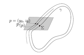
Figure 3. Poincaré return map.

Proposition 4.2.

Let $\gamma:[0,l]\rightarrow\mathbb{R}^{3}$, $\gamma(x)=(\gamma_{1}(x),\gamma_{2}(x),\gamma_{3}(x))$, be a closed $\xi$-asymptotic line, having a projection in a plane which is locally strictly convex curve. Let $\mathcal{P}$ be the Poincaré map associated to $\gamma$. Then $d\mathcal{P}_{(0,0)}=\mathcal{Q}(l)$, where $\mathcal{Q}(x)$ is solution of the following Cauchy problem:

$$\frac{d}{dx}\left(\mathcal{Q}(x)\right)=\mathcal{M}(x)\mathcal{Q}(x),\ \ \mathcal{Q}(0)=\mathcal{I},$$ (4.3)

where $\mathcal{I}$ is the identity matrix, and $\mathcal{M}(x)$, $\mathcal{Q}(x)$ are the matrices given by

$$\mathcal{M}(x)=\left(\begin{array}[]{cc}-\frac{e_{y}(x,0,0)}{2f(x,0,0)}&-\frac{e_{z}(x,0,0)}{2f(x,0,0)}\\ \left(A\right)_{y}(x,0,0)&\left(A\right)_{z}(x,0,0)\\ \end{array}\right),\mathcal{Q}(x)=\left(\begin{array}[]{cc}\frac{dy}{dy_{0}}(x,0,0)&\frac{dy}{dz_{0}}(x,0,0)\\ \frac{dz}{dy_{0}}(x,0,0)&\frac{dz}{dz_{0}}(x,0,0)\\ \end{array}\right),$$ (4.4)

where $A=-\frac{a}{c}$.

Proof.

To fix the notation suppose that $\gamma(0)=\gamma(l)$, $(\gamma_{1}^{\prime}(x),\gamma_{2}^{\prime}(x))\neq(0,0)$ and $\gamma_{1}^{\prime}(x)\gamma_{2}^{\prime\prime}(x)-\gamma_{2}^{\prime}(x)\gamma_{1}^{\prime\prime}(x)\neq 0$ for all $x$.

Let $(y(x,y_{0},z_{0}),z(x,y_{0},z_{0}))$ be solution of the Cauchy problem given by equation (4.2). Then, at $(y,z)=(0,0)$, $\frac{dy}{dx}(x,0,0)=\frac{dz}{dx}(x,0,0)=0$.

Differentiating the first equation of (4.2) with respect to $y_{0}$ (resp. $z_{0}$), it results that:

$$\begin{split}\frac{d}{dx}\left(\frac{dz}{dy_{0}}\right)=A_{y}\frac{dy}{dy_{0}}+A_{z}\frac{dz}{dy_{0}}+B\frac{d}{dx}\left(\frac{dy}{dy_{0}}\right)+\left(B_{y}\frac{dy}{dy_{0}}+B_{z}\frac{dz}{dy_{0}}\right)\frac{dy}{dx},\end{split}$$ (4.5)

respectively,

$$\begin{split}\frac{d}{dx}\left(\frac{dz}{dz_{0}}\right)=A_{y}\frac{dy}{dz_{0}}+A_{z}\frac{dz}{dz_{0}}+B\frac{d}{dx}\left(\frac{dy}{dz_{0}}\right)+\left(B_{y}\frac{dy}{dz_{0}}+B_{z}\frac{dz}{dz_{0}}\right)\frac{dy}{dx}.\end{split}$$ (4.6)

Differentiating the second equation of (4.2) with respect to $y_{0}$ (resp. $z_{0}$), it results that:

$$\begin{split}&e_{y}\frac{dy}{dy_{0}}+e_{z}\frac{dz}{dy_{0}}+2f\frac{d}{dx}\left(\frac{dy}{dy_{0}}\right)+2\left(f_{y}\frac{dy}{dy_{0}}+f_{z}\frac{dz}{dy_{0}}+g\frac{d}{dx}\left(\frac{dy}{dy_{0}}\right)\right)\frac{dy}{dx}\\ &+\left(g_{y}\frac{dy}{dy_{0}}+g_{z}\frac{dz}{dy_{0}}\right)\left(\frac{dy}{dx}\right)^{2}=0,\end{split}$$ (4.7)

respectively,

$$\begin{split}&e_{y}\frac{dy}{dz_{0}}+e_{z}\frac{dz}{dz_{0}}+2f\frac{d}{dx}\left(\frac{dy}{dz_{0}}\right)+2\left(f_{y}\frac{dy}{dz_{0}}+f_{z}\frac{dz}{dz_{0}}+g\frac{d}{dx}\left(\frac{dy}{dz_{0}}\right)\right)\frac{dy}{dx}\\ &+\left(g_{y}\frac{dy}{dz_{0}}+g_{z}\frac{dz}{dz_{0}}\right)\left(\frac{dy}{dx}\right)^{2}=0.\end{split}$$ (4.8)

Evaluating (4.5), (4.6), (4.7), (4.8) at $(y,z)=(0,0)$, it follows that:

$$\begin{split}&A_{y}\frac{dy}{dy_{0}}+A_{z}\frac{dz}{dy_{0}}=\frac{d}{dx}\left(\frac{dz}{dy_{0}}\right),\ \ e_{y}\frac{dy}{dy_{0}}+e_{z}\frac{dz}{dy_{0}}+2f\frac{d}{dx}\left(\frac{dy}{dy_{0}}\right)=0,\\ &A_{y}\frac{dy}{dz_{0}}+A_{z}\frac{dz}{dz_{0}}=\frac{d}{dx}\left(\frac{dz}{dz_{0}}\right),\ \ e_{y}\frac{dy}{dz_{0}}+e_{z}\frac{dz}{dz_{0}}+2f\frac{d}{dx}\left(\frac{dy}{dz_{0}}\right)=0.\end{split}$$ (4.9)

Then $\frac{d}{dx}\left(\mathcal{Q}(x)\right)=\mathcal{M}(x)\mathcal{Q}(x)$. Since $(y(0,y_{0},z_{0}),z(0,y_{0},z_{0}))=(y_{0},z_{0})$, it follows that $\mathcal{Q}(0)=\mathcal{I}$.

Since $\mathcal{P}(y_{0},z_{0})=(y(l,y_{0},z_{0}),z(l,y_{0},z_{0}))$, the first derivative $d\mathcal{P}_{(0,0)}$ is given by $\mathcal{Q}(l)$. ∎

4.2. Example of a hyperbolic closed finite type $\xi$-asymptotic line

An explicit example of a hyperbolic closed $\xi$-asymptotic line is given in the next result.

Theorem 4.3.

Let $\gamma:[0,2\pi]\rightarrow\mathbb{R}^{3}$, $\gamma(x)=(sin(x),cos(x),sin^{3}(x))$, see Fig. 4. Then it is a hyperbolic finite type $\xi$-asymptotic line of a suitable plane field.

Proof.

Let $\xi$ be a plane field orthogonal to the vector field $\xi$ given by (2.10), where $k_{0}(x)$ and $l_{0}(x)$ are given by (2.11). Let $k_{1}(x)$ given by (4.1), with $H(x)\equiv 1$. Then

$$k_{1}(x)=\frac{3(3cos^{2}(x)-1)sin(x)l_{1}(x)+24cos^{3}(x)-18cos(x)-2}{9cos^{6}(x)-18cos^{4}(x)+9cos^{2}(x)+1}.$$ (4.10)

By Proposition 4.1, $\gamma$ is a $\xi$-asymptotic line without parabolic points and $\mathcal{K}(x,0,0)=-1$. Performing the calculations, $e_{z}(x,0,0)=\mathcal{E}(x)+l_{2}(x)$. Solve $e_{z}(x,0,0)=0$ for $l_{2}(x)$. This vanishes the entry $\left(-\frac{e_{z}(x,0,0)}{2f(x,0,0)}\right)$ of $\mathcal{M}(x)$ given by Theorem 4.2. From (4.3), it follows that the eigenvalues of $d\mathcal{P}_{(0,0)}$ are given by

$${\rm exp}\left(\int_{0}^{2\pi}-\frac{e_{y}(x,0,0)}{2f(x,0,0)}dx\right)\;\;\;{\rm and}\;\;\;{\rm exp}\left(\int_{0}^{2\pi}A_{z}(x,0,0)dx\right).$$ (4.11)

Set $l_{1}(x)=cos(x)$. Then

$$\begin{split}A_{z}(x,0,0)&=9sin(x)cos^{8}(x)+54sin(x)cos^{6}(x)-9cos^{6}(x)-117sin(x)cos^{4}(x)\\ &+18cos^{4}(x)+55cos^{2}(x)sin(x)-9cos^{2}(x)-1.\end{split}$$ (4.12)

It follows that $\int_{0}^{2\pi}A_{z}(x,0,0)dx=-\frac{25\pi}{8}$. Let $k_{3}(x)=0$ and $k_{2}(x)$ a solution of the equation $e_{y}(x,0,0)+2f(x,0,0)=0$. It follows that

$$\int_{0}^{2\pi}\left(-\frac{e_{y}(x,0,0)}{2f(x,0,0)}\right)dx=2\pi.$$

∎

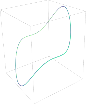
(a)

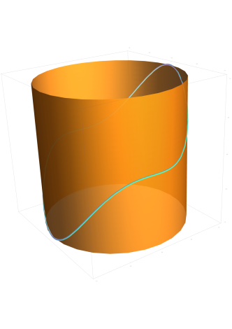
(b)

Figure 4. Finite type curve $\gamma(x)=(sin(x),cos(x),sin^{3}(x))$.

Authors:	Douglas H. da Cruz and Ronaldo A. Garcia
Address:	Instituto de Matemática e Estatística
	Universidade Federal de Goiás
	Campus Samambaia
	74690-900 - Goiânia -G0 - Brasil
	email: ragarcia@ufg.br

Appendix A A new proof of the Arnold’s Theorem

Here it will be given a geometric proof of Arnold’s Theorem.

Proof.

Let $\gamma$ be an asymptotic line of finite type $(u,u^{m},u^{n})$, $n\geq m$. Set $N(u)=(\gamma_{2}^{\prime}(u),-\gamma_{1}^{\prime}(u),0)$. Let

$$\alpha(u,v)=\gamma(u)+vN(u)+(k_{1}(u)v+k_{2}(u)v^{2}+k_{3}(u)v^{3}+\mathcal{O}^{4}(v))(\gamma^{\prime}\wedge N)(u).$$ (A.1)

Let

$$N_{\alpha}=\frac{\alpha_{u}\wedge\alpha_{v}}{|\alpha_{u}\wedge\alpha_{v}|}.$$ (A.2)

The implicit differential equations of the asymptotic lines of $\alpha$ is given by

$$edu^{2}+2fdudv+gdv^{2}=0,$$ (A.3)

where $e=\langle\alpha_{uu},N_{\alpha}\rangle$, $f=\langle\alpha_{uv},N_{\alpha}\rangle$ and $g=\langle\alpha_{vv},N_{\alpha}\rangle$.

Since $\gamma$ is an asymptotic line of $\alpha$, and parametrized by $v=0$, we have that $e(u,0)=0$. Then by equation (4.1) it follows that

$$k_{1}(u)=\frac{[(n-m)m^{2}u^{2(m-1)}+n-1]nu^{n-m}}{[1+m^{2}u^{2(m-1)}+n^{2}u^{2(n-1)}](m-1)m}.$$ (A.4)

Direct calculations shows that

$$f(u,0)=\frac{(n-m)(n-1)n(1+m^{2}u^{2(m-1)})^{2}u^{n-m-1}}{(m-1)m}.$$ (A.5)

It follows that $f(0,0)\neq 0$ if, and only if, $n=m+1$.

If $\gamma$ is a rotating space curve of finite type $(u,u^{m},u^{m+1})$, $m\geq 2$, set $N(u)=(\gamma_{2}^{\prime}(u),-\gamma_{1}^{\prime}(u),0)$ and let

$$\beta(u,v)=\gamma(u)+vN(u)+k_{1}(u)v(\gamma^{\prime}\wedge N)(u),$$ (A.6)

where $k_{1}(u)$ is given by (A.4) with $n=m+1$. Therefore, $e(u,0)=[\beta_{u},\beta_{v},\beta_{uu}](0,0)=0$ and $f(0,0)=[\beta_{u},\beta_{v},\beta_{uv}](0,0)=\frac{m+1}{m-1}\neq 0$. Then $\gamma$ is an asymptotic line, without parabolic points, of the surface parametrized by $\beta$ in a neighborhood of $(u,v)=(0,0)$. ∎

References

- [1] Geometry. II, volume 29 of Encyclopaedia of Mathematical Sciences. Springer-Verlag, Berlin, 1993. Spaces of constant curvature, A translation of Geometriya. II, Akad. Nauk SSSR, Vsesoyuz. Inst. Nauchn. i Tekhn. Inform., Moscow, 1988, Translation by V. Minachin [V. V. Minakhin], Translation edited by È. B. Vinberg.
- [2] Y. Aminov. The geometry of vector fields. Gordon and Breach Publishers, Amsterdam, 2000.
- [3] Y. Aminov. The geometry of submanifolds. Gordon and Breach Science Publishers, Amsterdam, 2001.
- [4] V. I. Arnold. Topological problems in the theory of asymptotic curves. Tr. Mat. Inst. Steklova, 225(Solitony Geom. Topol. na Perekrest.):11–20, 1999.
- [5] L. Euler. Recherches sur la courbure des surfaces. Mémoires de l’Académie des Sciences de Berlin, 16(119–143):9, 1760.
- [6] R. Garcia, C. Gutierrez, and J. Sotomayor. Structural stability of asymptotic lines on surfaces immersed in . Bull. Sci. Math., 123(8):599–622, 1999.
- [7] R. Garcia and J. Sotomayor. Structural stability of parabolic points and periodic asymptotic lines. Mat. Contemp., 12:83–102, 1997.
- [8] R. Garcia and J. Sotomayor. Differential equations of classical geometry, a qualitative theory. Publicações Matemáticas do IMPA. [IMPA Mathematical Publications]. Instituto Nacional de Matemática Pura e Aplicada (IMPA), Rio de Janeiro, 2009.
- [9] S. Izumiya, M. d. C. Romero Fuster, M. A. S. Ruas, and F. Tari. Differential geometry from a singularity theory viewpoint. World Scientific Publishing Co. Pte. Ltd., Hackensack, NJ, 2016.
- [10] S. G. Krantz. Convex analysis. CRC Press, 2015.
- [11] L. Nirenberg. Rigidity of a class of closed surfaces. In Nonlinear Problems (Proc. Sympos., Madison, Wis., 1962), pages 177–193. Univ. of Wisconsin Press, Madison, Wis., 1963.
- [12] J. Palis, Jr. and W. de Melo. Geometric theory of dynamical systems. Springer-Verlag, New York-Berlin, 1982. An introduction, Translated from the Portuguese by A. K. Manning.
- [13] E. R. Rozendorn. Surfaces of negative curvature. In Current problems in mathematics. Fundamental directions, Vol. 48 (Russian), Itogi Nauki i Tekhniki, pages 98–195. Akad. Nauk SSSR, Vsesoyuz. Inst. Nauchn. i Tekhn. Inform., Moscow, 1989.
- [14] A. Voss. Geometrische Interpretation der Differentialgleichung . Math. Ann., 16(4):556–559, 1880.