On Symbolic Approaches for Computing the Matrix Permanent

Abstract

Counting the number of perfect matchings in bipartite graphs, or equivalently computing the permanent of $0$-$1$ matrices, is an important combinatorial problem that has been extensively studied by theoreticians and practitioners alike. The permanent is #P-Complete; hence it is unlikely that a polynomial-time algorithm exists for the problem. Researchers have therefore focused on finding tractable subclasses of matrices for permanent computation. One such subclass that has received much attention is that of sparse matrices i.e. matrices with few entries set to $1$, the rest being $0$. For this subclass, improved theoretical upper bounds and practically efficient algorithms have been developed. In this paper, we ask whether it is possible to go beyond sparse matrices in our quest for developing scalable techniques for the permanent, and answer this question affirmatively. Our key insight is to represent permanent computation symbolically using Algebraic Decision Diagrams (ADDs). ADD-based techniques naturally use dynamic programming, and hence avoid redundant computation through memoization. This permits exploiting the hidden structure in a large class of matrices that have so far remained beyond the reach of permanent computation techniques. The availability of sophisticated libraries implementing ADDs also makes the task of engineering practical solutions relatively straightforward. While a complete characterization of matrices admitting a compact ADD representation remains open, we provide strong experimental evidence of the effectiveness of our approach for computing the permanent, not just for sparse matrices, but also for dense matrices and for matrices with “similar” rows.

1 Introduction

Constrained counting lies at the heart of several important problems in diverse areas such as performing Bayesian inference [46], measuring resilience of electrical networks [21], counting Kekule structures in chemistry [24], computing the partition function of monomer-dimer systems [27], and the like. Many of these problems reduce to counting problems on graphs. For instance, learning probabilistic models from data reduces to counting the number of topological sorts of directed acyclic graphs [57], while computing the partition function of a monomer-dimer system reduces to computing the number of perfect matchings of an appropriately defined bipartite graph [27]. In this paper, we focus on the last class of problems – that of counting perfect matchings in bipartite graphs. It is well known that this problem is equivalent to computing the permanent of the $0$-$1$ bi-adjacency matrix of the bipartite graph. We refer to these two problems interchangeably in the remainder of the paper.

Given an $n\times n$ matrix $\boldsymbol{A}$ with real-valued entries, the permanent of $\boldsymbol{A}$ is given by $perm(\boldsymbol{A})=\sum_{\sigma\in S_{n}}\prod_{i=1}^{n}a_{i,\sigma(i)}$, where $S_{n}$ denotes the symmetric group of all permutations of $1,\ldots n$. This expression is almost identical to that for the determinant of $\boldsymbol{A}$; the only difference is that the determinant includes the sign of the permutation in the inner product. Despite the striking resemblance of the two expressions, the complexities of computing the permanent and determinant are vastly different. While the determinant can be computed in time $\mathcal{O}(n^{2.4})$, Valiant [55] showed that computing the permanent of a $0$-$1$ matrix is #P-Complete, making a polynomial-time algorithm unlikely [54]. Further evidence of the hardness of computing the permanent was provided by Cai, Pavan and Sivakumar [11], who showed that the permanent is also hard to compute on average. Dell et al. [19] showed that there can be no algorithm with sub-exponential time complexity, assuming a weak version of the Exponential Time Hypothesis [2] holds.

The determinant has a nice geometric interpretation: it is the oriented volume of the parallelepiped spanned by the rows of the matrix. The permanent, however, has no simple geometric interpretation. Yet, it finds applications in a wide range of areas. In chemistry, the permanent and the permanental polynomial of the adjacency matrices of fullerenes [33] have attracted much attention over the years [12, 35, 13]. In constraint programming, solutions to All-Different constraints can be expressed as perfect matchings in a bipartite graph [44]. An estimate of the number of such solutions can be used as a branching heuristic to guide search [61, 43]. In physics, permanents can be used to measure quantum entanglement [59] and to compute the partition functions of monomer-dimer systems [27].

Since computing the permanent is hard in general, researchers have attempted to find efficient solutions for either approximate versions of the problem, or for restricted classes of inputs. In this paper, we restrict our attention to exact algorithms for computing the permanent. The asymptotically fastest known exact algorithm for general $n\times n$ matrices is Nijenhuis and Wilf’s version of Ryser’s algorithm [47, 39], which runs in time ${\Theta}(n\cdot 2^{n})$ for all matrices of size $n$. For matrices with bounded treewidth or clique-width [45, 15], Courcelle, Makowsky and Rotics [16] showed that the permanent can be computed in time linear in the size of the matrix, i.e., computing the permanent is Fixed Parameter Tractable (FPT). A large body of work is devoted to developing fast algorithms for sparse matrices, i.e. matrices with only a few entries set to non-zero values [49, 35, 29, 60] in each row. Note that the problem remains #P-Complete even when the input is restricted to matrices with exactly three $1$’s per row and column [9].

An interesting question to ask is whether we can go beyond sparse matrices in our quest for practically efficient algorithms for the permanent. For example, can we hope for practically efficient algorithms for computing the permanent of dense matrices, i.e., matrices with almost all entries non-zero? Can we expect efficiency when the rows of the matrix are “similar”, i.e. each row has only a few elements different from any other row (sparse and dense matrices being special cases)? Existing results do not seem to throw much light on these questions. For instance, while certain non-sparse matrices indeed have bounded clique-width, the aforementioned result of Courcelle et al [14, 16] does not yield practically efficient algorithms as the constants involved are enormous [25]. The hardness of non-sparse instances is underscored by the fact that SAT-based model counters do not scale well on these, despite the fact that years of research and careful engineering have enabled these tools to scale extremely well on a diverse array of problems. We experimented with a variety of CNF-encodings of the permanent on state-of-the-art counters like $\mathsf{D4}$ [34]. Strikingly, no combination of tool and encoding was able to scale to matrices even half the size of those solved by Ryser’s approach in the same time, despite the fact that Ryser’s approach has exponential complexity even in the best case.

In this paper, we show that practically efficient algorithms for the permanent can indeed be designed for large non-sparse matrices if the matrix is represented compactly and manipulated efficiently using a special class of data structures. Specifically, we propose using Algebraic Decision Diagrams [3] (ADDs) to represent matrices, and design a version of Ryser’s algorithm to work on this symbolic representation of matrices. This effectively gives us a symbolic version of Ryser’s algorithm, as opposed to existing implementations that use an explicit representation of the matrix. ADDs have been studied extensively in the context of formal verification, and sophisticated libraries are available for compact representation of ADDs and efficient implementation of ADD operations [51, 56]. The literature also contains compelling evidence that reasoning based on ADDs and variants scales to large instances of a diverse range of problems in practice, cf. [4, 22]. Our use of ADDs in Ryser’s algorithm leverages this progress for computing the permanent. Significantly, there are several sub-classes of matrices that admit compact representations using ADDs, and our algorithm works well for all these classes. Our empirical study provides evidence for the first time that the frontier of practically efficient permanent computation can be pushed well beyond the class of sparse matrices, to the classes of dense matrices and, more generally, to matrices with “similar” rows. Coupled with a technique known as early abstraction, ADDs are able to handle sparse instances as well. In summary, the symbolic approach to permanent computation shows promise for both sparse and dense classes of matrices, which are special cases of a notion of row-similarity.

The rest of the paper is organized as follows: in Section 2 we introduce ADDs and other concepts that we will use in this paper. We discuss related work in Section 3 and present our algorithm and analyze it in Section 4. Our empirical study is presented in Sections 5 and 6 and we conclude in Section 7.

2 Preliminaries

We denote by $\boldsymbol{A}=(a_{ij})$ an $n\times n$ $0$-$1$ matrix, which can also be interpreted as the bi-adjacency matrix of a bipartite graph $G_{\boldsymbol{A}}=(U\cup V,E)$ with an edge between vertex $i\in U$ and $j\in V$ iff $a_{ij}=1$. We will denote the $i$th row of $\boldsymbol{A}$ by $r_{i}$. A perfect matching in $G_{\boldsymbol{A}}$ is a subset $\mathcal{M}\subseteq E$, such that for all $v\in(U\cup V)$, exactly one edge $e\in\mathcal{M}$ is incident on $v$. We denote by $perm(\boldsymbol{A})$ the permanent of $\boldsymbol{A}$, and by $\#PM(G_{\boldsymbol{A}})$, the number of perfect matchings in $G$. A well known fact is that $perm(\boldsymbol{A})=\#PM(G_{\boldsymbol{A}})$, and we will use these concepts interchangeably when clear from context.

2.1 Algebraic Decision Diagrams

Let $X$ be a set of Boolean-valued variables. An Algebraic Decision Diagram (ADD) is a data structure used to compactly represent a function of the form $f:2^{X}\rightarrow\mathbb{R}$ as a Directed Acyclic Graph (DAG). ADDs were originally proposed as a generalization of Binary Decision Diagrams (BDDs), which can only represent functions of the form $g:2^{X}\rightarrow\{0,1\}$. Formally, an ADD is a $4$-tuple $(X,T,\pi,G)$ where $X$ is a set of Boolean variables, the finite set $T\subset\mathbb{R}$ is called the carrier set, $\pi:X\rightarrow\mathbb{N}$ is the diagram variable order, and $G$ is a rooted directed acyclic graph satisfying the following three properties:

1. Every terminal node of $G$ is labeled with an element of $T$.

2. Every non-terminal node of $G$ is labeled with an element of $X$ and has two outgoing edges labeled $0$ and $1$.

3. For every path in $G$, the labels of visited non-terminal nodes must occur in increasing order under $\pi$.

We use lower case letters $f,g,\ldots$ to denote both functions from Booleans to reals as well as the ADDs representing them. Many operations on such functions can be performed in time polynomial in the size of their ADDs. We list some such operations that will be used in our discussion.

• Product: The product of two ADDs representing functions $f:2^{X}\rightarrow\mathbb{R}$ and $g:2^{Y}\rightarrow\mathbb{R}$ is an ADD representing the function $f\cdot g:2^{X\cup Y}\rightarrow\mathbb{R}$, where $f\cdot g(\tau)$ is defined as $f(\tau\cap X)\cdot g(\tau\cap Y)$ for every $\tau\in 2^{X\cup Y}$,

• Sum: Defined in a way similar to the product.

• If-Then-Else (ITE): This is a ternary operation that takes as inputs a BDD $f$ and two ADDs $g$ and $h$. $ITE(f,g,h)$ represents the function $f\cdot g+\neg f\cdot h$, and the corresponding ADD is obtained by substituting $g$ for the leaf ’1’ of $f$ and $h$ for the leaf ’0’, and simplifying the resulting structure.

• Additive Quantification: The existential quantification operation for Boolean-valued functions can be extended to real-valued functions by replacing disjunction with addition as follows. The additive quantification of $f:2^{X}\rightarrow\mathbb{R}$ is denoted as $\exists x.f:2^{X\backslash\{x\}}\rightarrow\mathbb{R}$ and for $\tau\in 2^{X\backslash\{x\}}$, we have $\exists x.f(\tau)=f(\tau)+f(\tau\cup\{x\})$.

ADDs share many properties with BDDs. For example, there is a unique minimal ADD for a given variable order $\pi$, called the canonical ADD, and minimization can be performed in polynomial time. Similar to BDDs, the variable order can significantly affect the size of the ADD. Hence heuristics for finding good variable orders for BDDs carry over to ADDs as well. ADDs typically have lower recombination efficiency, i.e. number of shared nodes, vis-a-vis BDDs. Nevertheless, sharing or recombination of isomorphic sub-graphs in an ADD is known to provide significant practical advantages in representing matrices, vis-a-vis other competing data structures. The reader is referred to [3] for a nice introduction to ADDs and their applications.

2.2 Ryser’s Formula

The permanent of $\boldsymbol{A}$ can be calculated by the principle of inclusion-exclusion using Ryser’s formula: $perm(\boldsymbol{A})=(-1)^{n}\sum_{S\subseteq[n]}(-1)^{|S|}\prod_{i=1}^{n}\sum_{j\in S}a_{ij}.$ Algorithms implementing Ryser’s formula on an explicit representation of an arbitrary matrix $\boldsymbol{A}$ (not necessarily sparse) must consider all $2^{n}$ subsets of $[n]$. As a consequence, such algorithms have at least exponential complexity. Our experiments show that even the best known existing algorithm implementing Ryser’s formula for arbitrary matrices [39], which iterates over the subsets of $[n]$ in Gray-code sequence, consistently times out after $1800$ seconds on a state-of-the-art computing platform when computing the permanent of $n\times n$ matrices, with $n\geq 35$.

3 Related Work

Valiant showed that computing the permanent is $\#P$-complete [55]. Subsequently, researchers have considered restricted sub-classes of inputs in the quest for efficient algorithms for computing the permanent, both from theoretical and practical points of view. We highlight some of the important milestones achieved in this direction.

A seminal result is the Fisher-Temperly-Kastelyn algorithm [53, 30], which computes the number of perfect matchings in planar graphs in PTIME. This result was subsequently extended to many other graph classes (c.f. [41]). Following the work of Courcelle et al., a number of different width parameters have been proposed, culminating in the definition of ps-width [48], which is considered to be the most general notion of width [8]. Nevertheless, as with clique-width, it is not clear whether it lends itself to practically efficient algorithms. Bax and Franklin [5] gave a Las Vegas algorithm with better expected time complexity than Ryser’s approach, but requiring $\mathcal{O}(2^{n/2})$ space.

For matrices with at most $C\cdot n$ zeros, Servedio and Wan [49] presented a $(2-\varepsilon)^{n}$-time and $\mathcal{O}(n)$ space algorithm where $\varepsilon$ depends on $C$. Izumi and Wadayama [29] gave an algorithm that runs in time $\mathcal{O^{*}}(2^{(1-1/(\Delta\log\Delta))n})$, where $\Delta$ is the average degree of a vertex. On the practical side, in a series of papers, Liang, Bai and their co-authors [35, 36, 60] developed algorithms optimized for computing the permanent of the adjacency matrices of fullerenes, which are 3-regular graphs.

In recent years, practical techniques for propositional model counting (#SAT) have come of age. State-of-the-art exact model counters like $\mathsf{DSharp}$ [38] and $\mathsf{D4}$ [34] also incorporate techniques from knowledge compilation. A straightforward reduction of the permanent to #SAT uses a Boolean variable $x_{ij}$ for each $1$ in row $i$ and column $j$ of the input matrix $\boldsymbol{A}$, and imposes Exact-One constraints on the variables in each row and column. This gives the formula $F_{perm(\boldsymbol{A})}=\bigwedge_{i\in[n]}ExactOne(\{x_{ij}:a_{ij}=1\})\wedge\,\,\bigwedge_{j\in[n]}ExactOne(\{x_{ij}:a_{ij}=1\})$. Each solution to $F_{perm(\boldsymbol{A})}$ is a perfect matching in the underlying graph, and so the number of solutions is exactly the permanent of the matrix. A number of different encodings can be used for translating Exact-One constraints to Conjunctive Normal Form (see Section 5.1). We perform extensive comparisons of our tool with $\mathsf{D4}$ and $\mathsf{DSharp}$ with six such encodings.

4 Representing Ryser’s Formula Symbolically

As noted in Sec. 2, an explicit implementation of Ryser’s formula iterates over all $2^{n}$ subsets of columns and its complexity is in $\Theta(n\cdot 2^{n})$. Therefore, any such implementation takes exponential time even in the best case. A natural question to ask is whether we can do better through a careful selection of subsets over which to iterate. This principle was used for the case of sparse matrices by Servedio and Wan [49]. Their idea was to avoid those subsets for which the row-sum represented by the innermost summation in Ryser’s formula, is zero for at least one row, since those terms do not contribute to the outer sum in Ryser’s formula. Unfortunately, this approach does not help for non-sparse matrices, as very few subsets of columns (if any) will yield a zero row-sum.

It is interesting to ask if we can exploit similarity of rows (instead of sparsity) to our advantage. Consider the ideal case of an $n\times n$ matrix with identical rows, where each row has $k~{}(\leq n)$ $1$s. For any given subset of columns, the row-sum is clearly the same for all rows, and hence the product of all row-sums is simply the $n^{th}$ power of the row-sum of one row. Furthermore, there are only $k+1$ distinct values ($0$ through $k$) of the row-sum, depending on which subset of columns is selected. The number of $r$-sized column subsets that yield row-sum $j$ is clearly ${k\choose j}\cdot{n-k\choose r-j}$, for $0\leq j\leq k$ and $j\leq r\leq n-k+j$. Thus, we can directly compute the permanent of the matrix via Ryser’s formula as $perm(\boldsymbol{A})=(-1)^{n}\sum_{j=0}^{k}\sum_{r=j}^{n-k+j}(-1)^{r}{k\choose j}\cdot{n-k\choose r-j}\cdot j^{n}$. This equation has a more compact representation than the explicit implementation of Ryser’s formula, since the outer summation is over $(k+1).(n-k+1)$ terms instead of $2^{n}$ terms.

Drawing motivation from the above example, we propose using memoization to simplify the permanent computation of matrices with similar rows. Specifically, if we compute and store the row-sums for a subset $S_{1}\subset[n]$ of columns, then we can potentially reuse this information when computing the row-sums for subsets $S_{2}\supset S_{1}$. We expect storage requirements to be low when the rows are similar, as the partial sums over identical parts of the rows will have a compact representation, as shown above.

While we can attempt to hand-craft a concrete algorithm using this idea, it turns out that ADDs fit the bill perfectly. We introduce Boolean variables $x_{j}$ for each column $1\leq j\leq n$ in the matrix. We can represent the summand $(-1)^{|S|}\prod_{i=1}^{n}\sum_{j\in S}a_{ij}$ in Ryser’s formula as a function $f_{Ryser}:2^{X}\rightarrow\mathbb{R}$ where for a subset of columns $\tau\in 2^{X}$, we have $f_{Ryser}(\tau)=(-1)^{|\tau|}\prod_{i=1}^{n}\sum_{j\in\tau}a_{ij}$. The outer sum in Ryser’s formula is then simply the Additive Quantification of $f_{Ryser}$ over all variables in $X$. The permanent can thus be denoted by the following equation:

$$perm(\boldsymbol{A})=(-1)^{n}\,\,.\,\,\exists x_{1},x_{2},\ldots x_{n}.(f_{Ryser})$$ (1)

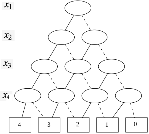
(a)

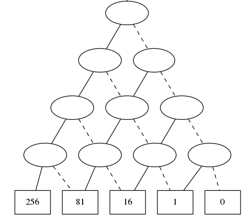
(b)

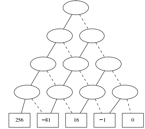
(c)

Figure 1: (a) $f_{RS}$, (b) $f_{RSP}$ and (c) $f_{Ryser}$ for a $4\times 4$ matrix of all 1s

We can construct an ADD for $f_{Ryser}$ incrementally as follows:

• Step 1: For each row $r_{i}$ in the matrix, construct the Row-Sum ADD $f_{RS}^{r_{i}}$ such that $f_{RS}^{r_{i}}(\tau)=\sum_{j:a_{ij}=1}\mathbbm{1}_{\tau}(x_{j})$, where $\mathbbm{1}_{\tau}(x_{j})$ is the indicator function taking the value 1 if $x_{j}\in\tau$, and zero otherwise. This ADD can be constructed by using the sum operation on the variables $x_{j}$ corresponding to the $1$ entries in row $r_{i}$.

• Step 2: Construct the Row-Sum-Product ADD $f_{RSP}=\prod_{i=1}^{n}f_{RS}^{r_{i}}$ by applying the product operation on all the Row-Sum ADDs

• Step 3: Construct the Parity ADD $f_{PAR}=ITE(\bigoplus_{j=1}^{n}x_{j},-1,+1)$, where $\bigoplus$ represents exclusive-or. This ADD represents the $(-1)^{|S|}$ term in Ryser’s formula.

• Step 4: Construct $f_{Ryser}=f_{RSP}.f_{PAR}$ using the product operation.

Finally, we can additively quantify out all variables in $f_{Ryser}$ and multiply the result by $(-1)^{n}$ to get the permanent, as given by Equation 1.

The size of the ADD $f_{RSP}$ will be the smallest when the ADDs $f_{RS}^{r_{i}}$ are exactly the same for all rows $r_{i}$, i.e. when all rows of the matrix are identical. In this case, the ADDs $f_{RS}^{r_{i}}$ and $f_{RSP}$ will be isomorphic; the values at the leaves of $f_{RSP}$ will simply be the $n^{th}$ power of the values at the corresponding leaves of $f_{RS}^{r_{i}}$. An example illustrating this for a $4\times 4$ matrix of all $1$s is shown in Fig. 1. Each level of the ADDs in this figure corresponds to a variable (shown on the left) for a column of the matrix. A solid edge represents the ’true’ branch while a dotted edge represents the ’false’ branch. Observe that sharing of isomorphic subgraphs allows each of these ADDs to have $10$ internal nodes and $5$ leaves, as opposed to $15$ internal nodes and $16$ leaves that would be needed for a complete binary tree based representation.

The ADD representation is thus expected to be compact when the rows are “similar”. Dense matrices can be thought of as a special case: starting with a matrix of all $1$s (which clearly has all rows identical), we change a few $1$s to $0$s. The same idea can be applied to sparse matrices as well: starting with a matrix of all $0$s (once again, identical rows), we change a few $0$s to $1$s. The case of very sparse matrices is not interesting, however, as the permanent (or equivalently, count of perfect matchings in the corresponding bipartite graph) is small and can be computed by naive enumeration. Interestingly, our experiments show that as we reduce the sparsity of the input matrix, constructing $f_{RSP}$ and $f_{Ryser}$ in a monolithic fashion as discussed above fails to scale, since the sizes of ADDs increase very sharply. Therefore we need additional machinery.

First, we rewrite Equation 1 in terms of the intermediate ADDs as:

$$perm(\boldsymbol{A})=(-1)^{n}\,\,.\,\,\exists x_{1},x_{2},\ldots x_{n}.\left(f_{PAR}\cdot\prod_{i=1}^{n}f_{RS}^{r_{i}}\right)$$ (2)

We then employ the principle of early abstraction to compute $f_{Ryser}$ incrementally. Note that early abstraction has been used successfully in the past in the context of SAT solving [42], and recently for weighted model counting using ADDs in a technique called $\mathsf{ADDMC}$ [20]. The formal statement of the principle of early abstraction is given in the following theorem.

Theorem 4.1

[20] Let $X$ and $Y$ be sets of variables and $f:2^{X}\rightarrow\mathbb{R}$, $g:2^{Y}\rightarrow\mathbb{R}$. For all $x\in X\setminus Y$, we have $\exists_{x}(f\cdot g)=(\exists_{x}(f))\cdot g$

Since the product operator is associative and additive quantification is commutative, we can rearrange the terms of Equation 2 in order to apply early abstraction. This idea is implemented in Algorithm $\mathsf{RysersADD}$, which is motivated by the weighted model counting algorithm in [20].

Algorithm 1 $\mathsf{RysersADD}(\boldsymbol{A},\pi,\eta)$

1:$m\leftarrow max_{x\in X}\,\,\eta(x)$;

2:for $i=m,m-1,\ldots,1$ do

3:     $\kappa_{i}\leftarrow\{f_{RS}^{r}:r$ is a row in $\boldsymbol{A}$ and $\mathsf{clusterRank}(r,\eta)=i\}$;

4:$f_{Ryser}\leftarrow f_{PAR}$; $\triangleright$ $f_{PAR}$ and each $f_{RS}^{r}$ are constructed using the diagram variable order $\pi$

5:for $i=1,2,\ldots,m$ do

6:     if $\kappa_{i}\neq\emptyset$ then

7:         for $g\in\kappa_{i}$ do

8:              $f_{Ryser}\leftarrow f_{Ryser}\cdot g$;          

9:         for $x\in Vars(f_{Ryser})$ do

10:              if $x\not\in(Vars(\kappa_{i+1})\cup\ldots\cup Vars(\kappa_{m}))$ then

11:                  $f_{Ryser}\leftarrow\exists_{x}(f_{Ryser})$                             

12:return $(-1)^{n}\times f_{Ryser}(\emptyset)$

Algorithm $\mathsf{RysersADD}$ takes as input a 0-1 matrix $\boldsymbol{A}$, a diagram variable order $\pi$ and a cluster rank-order $\eta$. $\eta$ is an ordering of variables which is used to heuristically partition rows of $\boldsymbol{A}$ into clusters using a function $\mathsf{clusterRank}$, where all rows in a cluster get the same rank. Intuitively, rows that are almost identical are placed in the same cluster, while those that differ significantly are placed in different clusters. Furthermore, the clusters are ordered such that there are non-zero columns in cluster $i$ that are absent in the set of non-zero columns in clusters with rank $>i$. As we will soon see, this facilitates keeping the sizes of ADDs under control by applying early abstraction.

Algorithm $\mathsf{RysersADD}$ proceeds by first partitioning the Row-Sum ADDs of the rows $\boldsymbol{A}$ into clusters according to their cluster rank in line 3. Each Row-Sum ADD is constructed according to the diagram variable order $\pi$. The ADD $f_{Ryser}$ is constructed incrementally, starting with the Parity ADD in line 4, and multiplying the Row-Sum ADDs in each cluster $\kappa_{i}$ in the loop at line 7. However, unlike the monolithic approach, early abstraction is carried out within the loop at line 9. Finally, when the execution reaches line 12, all variables representing columns of the input matrix have been abstracted out. Therefore, $f_{Ryser}$ is an ADD with a single leaf node that contains the (possibly negative) value of the permanent. Following Equation 2, the algorithm returns the product of $(-1)^{n}$ and $f_{Rsyer}(\emptyset)$.

The choice of the function $\mathsf{clusterRank}$ and the cluster rank-order $\eta$ significantly affect the performance of the algorithm. A number of heuristics for determining $\mathsf{clusterRank}$ and $\eta$ have been proposed in literature, such as Bucket Elimination [18], and Bouquet’s Method [7] for cluster ranking, and MCS [52], LexP [32] and LexM [32] for variable ordering. Further details and a rigorous comparison of these heuristics are presented in [20]. Note that if we assign the same cluster rank to all rows of the input matrix, Algorithm $\mathsf{RysersADD}$ reduces to one that constructs all ADDs monolithically, and does not benefit from early abstraction.

4.1 Implementation Details

We implemented Algorithm 1 using the library Sylvan [56] since unlike CUDD [51], Sylvan supports arbitrary precision arithmetic – an essential feature to avoid overflows when the permanent has a large value. Sylvan supports parallelization of ADD operations in a multi-core environment. In order to leverage this capability, we created a parallel version of $\mathsf{RysersADD}$ that differs from the sequential version only in that it uses the parallel implementation of ADD operations natively provided by Sylvan. Note that this doesn’t require any change to Algorithm $\mathsf{RysersADD}$, except in the call to Sylvan functions. While other non-ADD-based approaches to computing the permanent can be parallelized as well, we emphasize that it is a non-trivial task in general, unlike using Sylvan. We refer to our sequential and parallel implementations for permanent computation as $\mathsf{RysersADD}$ and $\mathsf{RysersADD{\text{-}}P}$ respectively, in the remainder of the discussion. We implemented our algorithm in C++, compiled under GCC v6.4 with the O3 flag. We measured the wall-times for both algorithms. Sylvan also supports arbitrary precision floating point computation, which makes it easy to extend $\mathsf{RysersADD}$ for computing permanent of real-valued matrices. However, we leave a detailed investigation of this for future work.

5 Experimental Methodology

The objective of our empirical study was to evaluate $\mathsf{RysersADD}$ and $\mathsf{RysersADD{\text{-}}P}$ on randomly generated instances (as done in [36]) and publicly available structured instances (as done in [35, 60]) of $0$-$1$ matrices.

5.1 Algorithm Suite

As noted in Section 3, a number of different algorithms have been reported in the literature for computing the permanent of sparse matrices. Given resource constraints, it is infeasible to include all of these in our experimental comparisons. This is further complicated by the fact that many of these algorithms appear not to have been implemented (eg: [49, 29]), or the code has not been made publicly accessible (eg:  [35, 60]). A fair comparison would require careful consideration of several parameters like usage of libraries, language of implementation, suitability of hardware etc. We had to arrive at an informed choice of algorithms, which we list below along with our rationale:

• $\mathsf{RysersADD}$ and $\mathsf{RysersADD{\text{-}}P}$: For the dense and similar rows cases, we use the monolithic approach as it is sufficient to demonstrate the scalability of our ADD-based approach. For sparse instances, we employ Bouquet’s Method (List) [7] clustering heuristic along with MCS cluster rank-order [52] and we keep the diagram variable order the same as the indices of columns in the input matrix (see [20] for details about the heuristics). We arrived at these choices through preliminary experiments. We leave a detailed comparison of all combinations for future work.

• Explicit Ryser’s Algorithm: We implemented Nijenhuis and Wilf’s version [39] of Ryser’s formula using Algorithm H from [31] for generating the Gray code sequence. Our implementation, running on a state-of-the-art computing platform (see Section 5.2), is able to compute the permanent of all matrices with $n\leq 25$ in under 5 seconds. For $n=30$, the time shoots up to approximately $460$ seconds and for $n\geq 34$, the time taken exceeds 1800 seconds (time out for our experiments). Since the performance of explicit Ryser’s algorithm depends only on the size of the matrix, and is unaffected by its structure, sparsity or row-similarity, this represents a complete characterization of the performance of the explicit Ryser’s algorithm. Hence, we do not include it in our plots.

• Propositional Model Counters: Model counters that employ techniques from SAT-solving as well as knowledge compilation, have been shown to scale extremely well on large CNF formulas from diverse domains. Years of careful engineering have resulted in counters that can often outperform domain-specific approaches. We used two state-of-the-art exact model counters, viz. $\mathsf{D4}$ [34] and $\mathsf{DSharp}$ [38], for our experiments. We experimented with 6 different encodings for At-Most-One constraints: (1) Pairwise [6], (2) Bitwise [6], (3) Sequential Counter [50], (4) Ladder [23, 1], (5) Modulo Totalizer [40] and (6) Iterative Totalizer [37]. We also experimented with $\mathsf{ADDMC}$, an ADD-based model counter [20]. However, it failed to scale beyond matrices of size $25$; ergo we do not include it in our study.

We were unable to include the parallel #SAT counter countAtom [10] in our experiments, owing to difficulties in setting it up on our compute set-up. However, we could run countAtom on a slightly different set-up with 8 cores instead of 12, and 16GB memory instead of 48 on a few sampled dense and similar-row matrix instances. Our experiments showed that countAtom timed out on all these cases. We leave a more thorough and scientific comparison with countAtom for future work.

5.2 Experimental Setup

Each experiment (sequential or parallel) had exclusive access to a Westemere node with 12 processor cores running at 2.83 GHz with 48 GB of RAM. We capped memory usage at 42 GB for all tools. We implemented explicit Ryser’s algorithm in C++, compiled with GCC v6.4 with O3 flag. The $\mathsf{RysersADD}$ and $\mathsf{RysersADD{\text{-}}P}$ algorithms were implemented as in Section 4.1. $\mathsf{RysersADD{\text{-}}P}$ had access to all $12$ cores for parallel computation. We used the python library PySAT [28] for encoding matrices into CNF. We set the timeout to $1800$ seconds for all our experiments. For purposes of reporting, we treat a memory out as equivalent to a time out.

Table 1: Parameters used for generating random matrices

Experiment	Matrix Size n	$C_{f}$, where $C_{f}\cdot n$ matrix entries flipped	Starting Matrix Row Density $\rho$	#Instances	Total Benchmarks
Dense	30, 40, 50, 60, 70	1, 1.1, 1.2, 1.3, 1.4	1	20	500
Sparse	30, 40, 50, 60, 70	3.9, 4.3, 4.7, 5.1, 5.5	0	20	500
Similar	40, 50, 60, 70, 80	1, 1.1, 1.2, 1.3, 1.4	0.7, 0.8, 0.9	15	1125

5.3 Benchmarks

The parameters used for generating random instances are summarized in Table 1. We do not include matrices with $n<30$ since the explicit Ryser’s algorithm suffices (and often performs the best) for such matrices. The upper bound for $n$ was chosen such that the algorithms in our suite either timed out or came close to timing out. For each combination of parameters, random matrix instances were sampled as follows:

1. We started with an $n\times n$ matrix, where the first row had $\rho\cdot n$ $1$s at randomly chosen column positions, and all other rows were copies of the first row.

2. $C_{f}\cdot n$ randomly chosen entries in the starting matrix are flipped i.e. $0$ flipped to $1$ and vice versa.

For the dense case, we start with a matrix of all $1$s while for the sparse case, we start with a matrix of all $0$s, and used intermediate row density values for the similar-rows case. We chose higher values for $C_{f}$ in the sparse case because for low values, the bipartite graph corresponding to the generated matrix had very few perfect matchings (if any), and these could be simply counted by enumeration. We generated a total of $2125$ benchmarks covering a broad range of parameters. For all generated instances, we ensured that there was at least one perfect matching, since the case with zero perfect matchings can be easily solved in polynomial time by algorithms like Hopcroft-Karp [26]. In order to avoid spending inordinately large time on failed experiments, if an algorithm timed out on all generated random instances of a particular size, we also report a time out for that algorithm on all larger instances of that class of matrices. We also double-check this by conducting experiments with the same algorithm on a few randomly chosen larger instances.

The SuiteSparse Matrix Collection [17] is a well known repository of structured sparse matrices that arise from practical applications. We found $26$ graphs in this suite with vertex count between $30$ and $100$, of which $18$ had at least one perfect matching. Note that these graphs are not necessarily bipartite; however, their adjacency matrices can be used as benchmarks for computing the permanent. A similar approach was employed in [58] as well.

Fullerenes are carbon molecules whose adjacency matrices have been used extensively by Liang et al. [35, 58, 60] for comparing tools for the permanent. We were able to find the adjacency matrices of $C_{60}$ and $C_{100}$, and have used these in our experiments.

6 Results

We first study the variation of running time of $\mathsf{RysersADD}$ with the size of ADDs involved. Then we compare the running times of various algorithms on sparse, dense and similar-row matrices, as well as on instances from SuiteSparse Matrix Collection and on adjacency matrices of fullerenes $C_{60}$ and $C_{100}$. The total computational effort of our experiments exceeds $2500$ hours of wall clock time on dedicated compute nodes.

6.1 ADD size vs time taken by $\mathsf{RysersADD}$

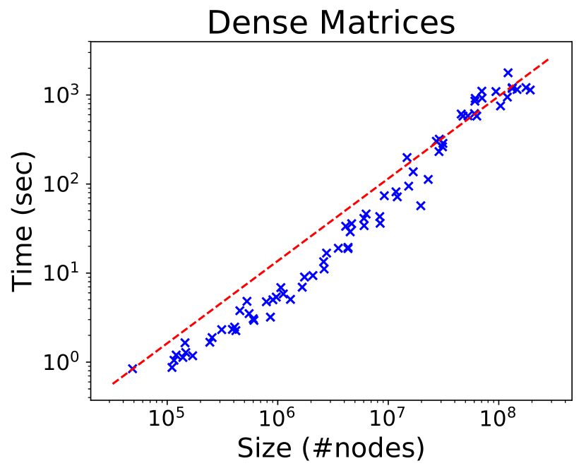
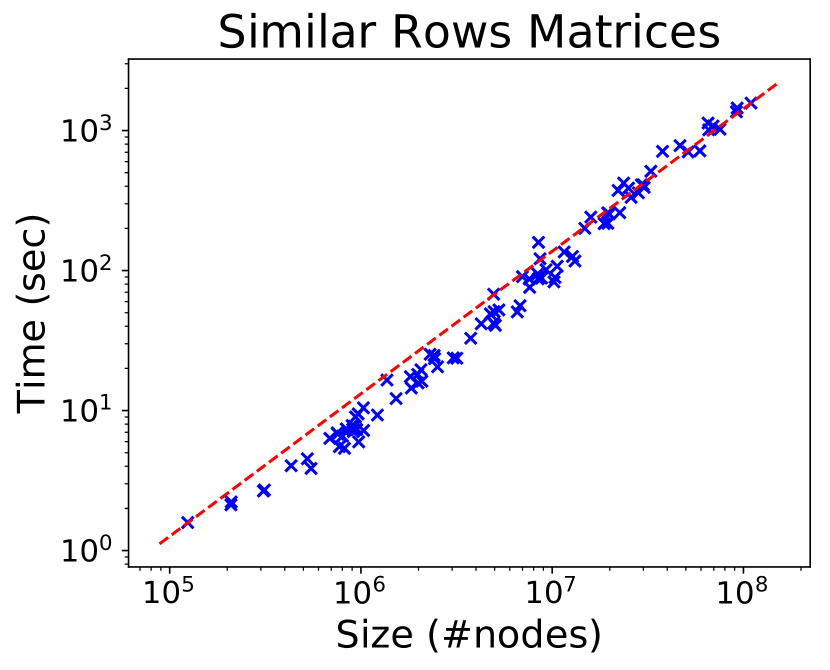
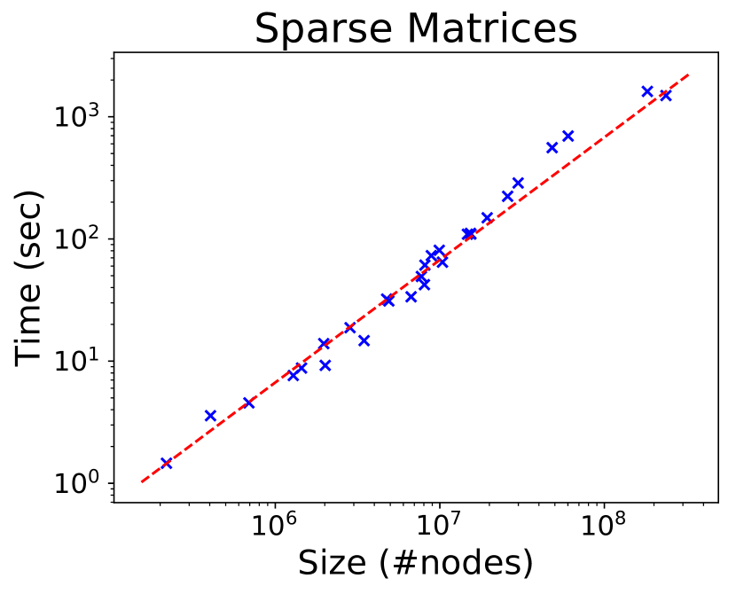
Figure 2: Comparison of ADD Size vs. Time taken for a subset of random benchmarks

In order to validate the hypothesis that the size of the ADD representation is a crucial determining factor of the performance of $\mathsf{RysersADD}$, we present $3$ scatter-plots (Fig. 2) for a subset of $100$ instances, of each of the dense, sparse and similar-rows cases. In each case, the $100$ instances cover the entire range of $C_{f}$ and $n$ used in Table 1, and we plot times only for instances that didn’t time out. The plots show that there is very strong correlation between the number of nodes in the ADDs and the time taken for computing the permanent, supporting our hypothesis.

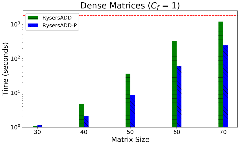
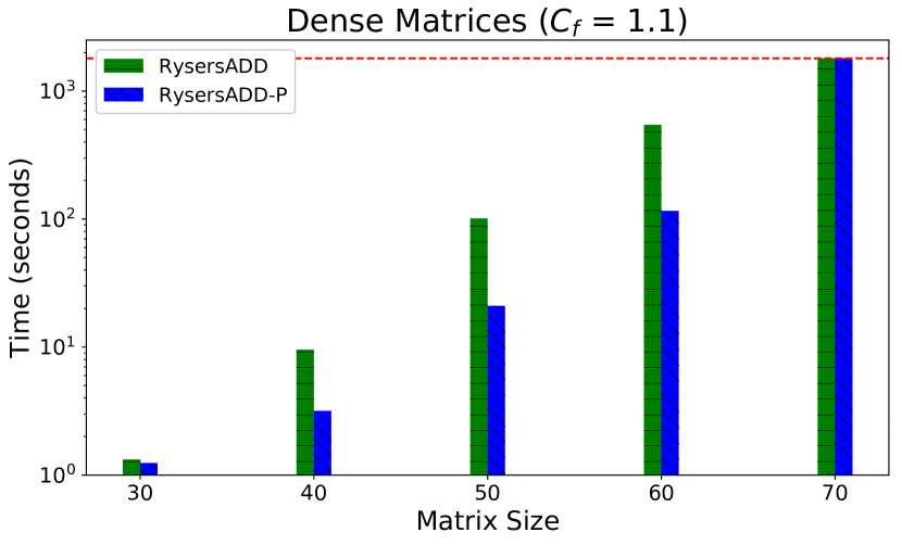
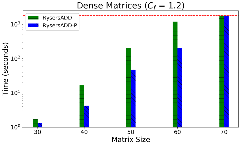
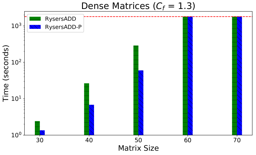
Figure 3: Performance on Dense Matrices. $\mathsf{D4}$, $\mathsf{DSharp}$ (not shown) timeout on all instances

6.2 Performance on dense matrices

We plot the median running time of $\mathsf{RysersADD}$ and $\mathsf{RysersADD{\text{-}}P}$ against the matrix size $n$ for dense matrices with $C_{f}\in\{1,1.1,1.2,1.3\}$ in Fig. 3. We only show the running times of $\mathsf{RysersADD}$ and $\mathsf{RysersADD{\text{-}}P}$, since $\mathsf{D4}$ and $\mathsf{DSharp}$ were unable to solve any instance of size $30$ for all $6$ encodings. We observe that the running time of both the ADD-based algorithms increases with $C_{f}$. This trend continues for $C_{f}=1.4$, which we omit for lack of space. $\mathsf{RysersADD{\text{-}}P}$ is noticeably faster than $\mathsf{RysersADD}$, indicating that the native parallelism provided by Sylvan is indeed effective.

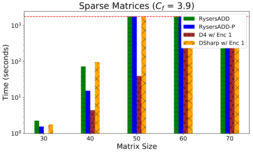
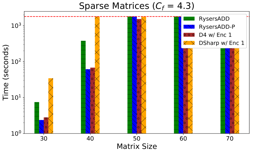
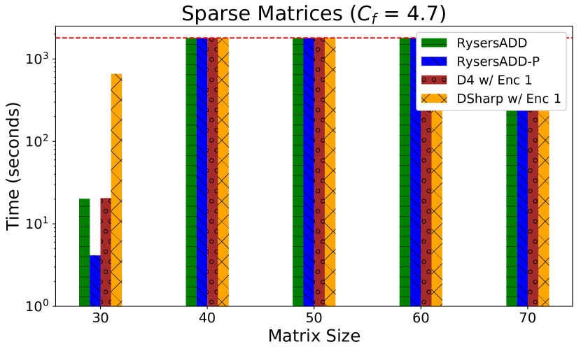
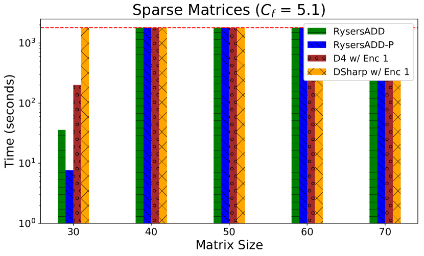
Figure 4: Performance on Sparse Matrices

6.3 Performance on sparse matrices

Fig. 4 depicts the median running times of the algorithms for sparse matrices with $C_{f}\in\{3.9,4.3,4.7,5.1\}$. We plot the running time of the ADD-based approaches with early abstraction (see Sec. 5.1). Monolithic variants (not shown) time out on all instances with $n\geq 40$. For $\mathsf{D4}$ and $\mathsf{DSharp}$, we plot the running times only for Pairwise encoding of At-Most-One constraints, since our preliminary experiments showed that it substantially outperformed other encodings. We see that $\mathsf{D4}$ is the fastest when sparsity is high i.e. for $C_{f}\leq 4.3$, but for $C_{f}\geq 4.7$ the ADD-based methods are the best performers. $\mathsf{DSharp}$ is outperformed by the remaining $3$ algorithms in general.

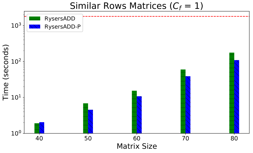
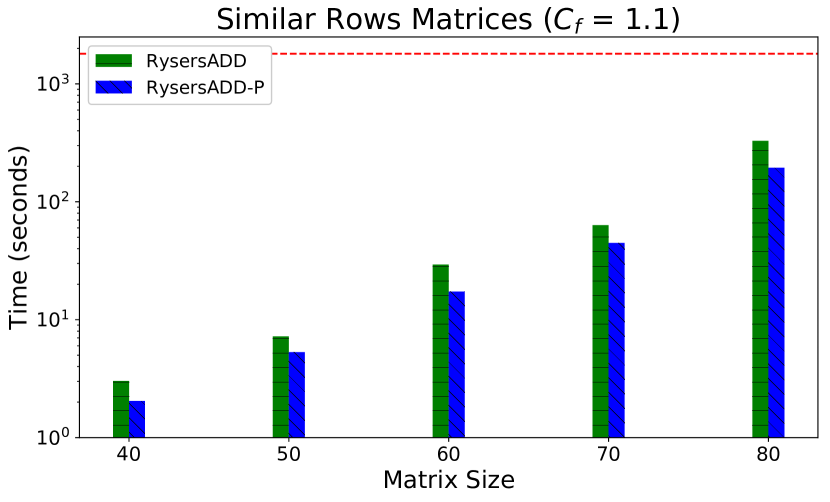
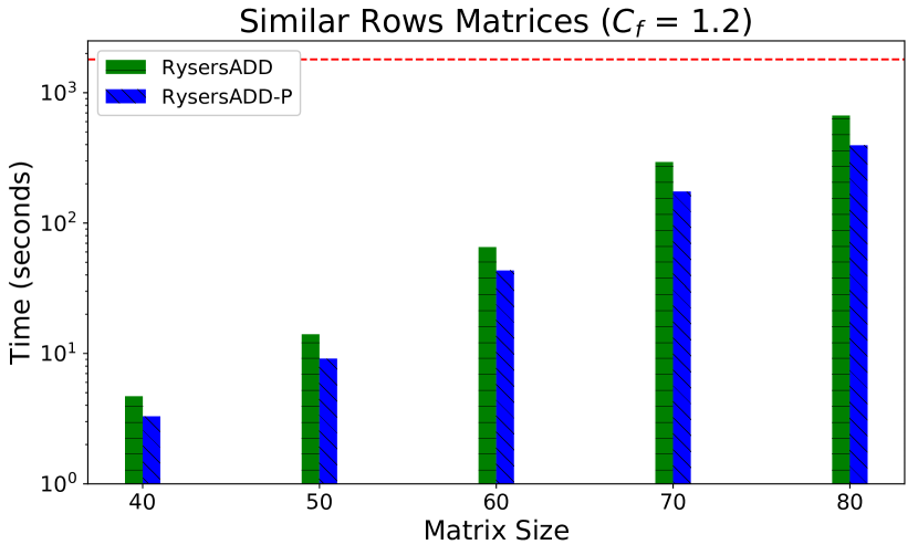
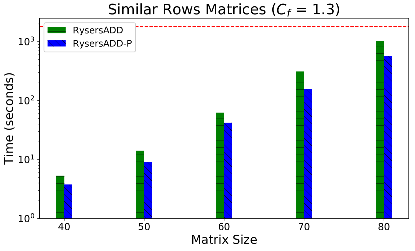
Figure 5: Performance on similar-rows matrices. $\mathsf{D4}$, $\mathsf{DSharp}$ (not shown) timeout on all instances.

6.4 Performance on similar-row matrices

Fig. 5 shows plots of the median running time on similar-row matrices with $C_{f}=\{1,1.1,1.2,1.3\}$. We only present the case when $\rho=0.8$, since the plots are similar when $\rho\in\{0.7,0.9\}$. As in the case of dense matrices, $\mathsf{D4}$ and $\mathsf{DSharp}$ were unable to solve any instance of size $40$, and hence we only show plots for $\mathsf{RysersADD}$ and $\mathsf{RysersADD{\text{-}}P}$. The performance of both tools is markedly better than in the case of dense matrices, and they scale to matrices of size $80$ within the $1800$ second timeout.

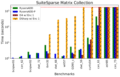
Figure 6:

6.5 Performance on SuiteSparse Matrix Collection

We report the performance of algorithms $\mathsf{RysersADD}$, $\mathsf{RysersADD{\text{-}}P}$, $\mathsf{D4}$ and $\mathsf{DSharp}$ on $13$ representative graphs from the SuiteSparse Matrix Collection in Fig. 6. Except for the first $4$ instances, which can be solved in under 5 seconds by all algorithms, we find that $\mathsf{D4}$ is the fastest in general, while the ADD-based algorithms outperform $\mathsf{DSharp}$. Notably, on the instance ”can_61”, both $\mathsf{D4}$ and $\mathsf{DSharp}$ time out while $\mathsf{RysersADD}$ and $\mathsf{RysersADD{\text{-}}P}$ solve it comfortably within the alloted time. We note that the instance ”can_61” has roughly $9n$ $1$s, while $\mathsf{D4}$ is the best performer on instances where the count of $1$s in the matrix lies between $4n$ and $6n$.

Table 2: Running Times on the fullerene $C_{60}$. EA: Early Abstraction Mono: Monolithic

Tool	$\mathsf{D4}$						$\mathsf{DSharp}$						$\mathsf{RysersADD}$		$\mathsf{RysersADD{\text{-}}P}$
Encoding / Mode	1	2	3	4	5	6	1	2	3	4	5	6	EA	Mono	EA	Mono
Time (sec)	94.8	150.5	150.6	136	158	156	TimeOut						96.4	TimeOut	57.1	TimeOut

6.6 Performance on fullerene adjacency matrices

We compared the performance of the algorithms on the adjacency matrices of the fullerenes $C_{60}$ and $C_{100}$. All the algorithms timed out on $C_{100}$. The results for $C_{60}$ are shown in Table 2. The columns under $\mathsf{D4}$ and $\mathsf{DSharp}$ correspond to $6$ different encodings of At-Most-One constraints (see Sec. 5.1). It can be seen that $\mathsf{RysersADD{\text{-}}P}$ performs the best on this class of matrices, followed by $\mathsf{D4}$. The utility of early abstraction is clearly evident, as the monolithic approach times out in both cases.

Discussion: Our experiments show the effectiveness of the symbolic approach on dense and similar-rows matrices, where neither $\mathsf{D4}$ nor $\mathsf{DSharp}$ are able to solve even a single instance. Even for sparse matrices, we see that decreasing sparsity has lesser effect on the performance of ADD-based approaches as compared to $\mathsf{D4}$. This trend is confirmed by ”can_61” in the SuiteSparse Matrix Collection as well, where despite the density of $1$s being $9n$, $\mathsf{RysersADD}$ and $\mathsf{RysersADD{\text{-}}P}$ finish well within timeout, unlike $\mathsf{D4}$. In the case of fullerenes, we note that the algorithm in [35] solved $C_{60}$ in 355 seconds while the one in [60] took 5 seconds, which are in the vicinity of the times reported in Table 2. While this is not an apples-to-apples comparison owing to differences in the computing platform, it indicates that the performance of general-purpose algorithms like $\mathsf{RysersADD}$ and $\mathsf{D4}$ can be comparable to that of application-specific algorithms.

7 Conclusion

In this work we introduced a symbolic algorithm called $\mathsf{RysersADD}$ for permanent computation based on augmenting Ryser’s formula with Algebraic Decision Diagrams. We demonstrated, through rigorous experimental evaluation, the scalability of $\mathsf{RysersADD}$ on both dense and similar-rows matrices, where existing approaches fail. Coupled with the technique of early abstraction [20], $\mathsf{RysersADD}$ performs reasonably well even on sparse matrices as compared to dedicated approaches. In fact, it may be possible to optimize the algorithm even further, by evaluating other heuristics used in [20]. We leave this for future work. Our work also re-emphasizes the versatility of ADDs and opens the door for their application to other combinatorial problems.

It is an interesting open problem to obtain a complete characterization of the class of matrices for which ADD representation of Ryser’s formula is succinct. Our experimental results for dense matrices hint at the possibility of improved theoretical bounds similar to those obtained in earlier work on sparse matrices. Developing an algorithm for general matrices that is exponentially faster than Ryser’s approach remains a long-standing open problem [29], and obtaining better bounds for non-sparse matrices would be an important first step in this direction.

References

- [1] C. Ansótegui and F. Manya. Mapping problems with finite-domain variables to problems with boolean variables. In International Conference on Theory and Applications of Satisfiability Testing, pages 1–15. Springer, 2004.
- [2] S. Arora and B. Barak. Computational Complexity: A Modern Approach. Cambridge Univ. Press, 2009.
- [3] R. Bahar, E. Frohm, C. Gaona, G. Hachtel, E. Macii, A. Pardo, and F. Somenzi. Algebraic decision diagrams and their applications. Journal of Formal Methods in Systems Design, 10(2/3):171–206, 1997.
- [4] R. Bahar, E. Frohm, C. Gaona, G. Hachtel, E. Macii, A. Pardo, and F. Somenzi. Algebraic decision diagrams and their applications. Journal of Formal Methods in Systems Design, 10(2/3):171–206, April/May 1997.
- [5] E. Bax and J. Franklin. A permanent algorithm with exp [(n1/3/2ln (n))] expected speedup for 0-1 matrices. Algorithmica, 32(1):157–162, 2002.
- [6] A. Biere, M. Heule, H. van Maaren, and T. Walsh. Handbook of Satisfiability: Volume 185 Frontiers in Artificial Intelligence and Applications. IOS Press, Amsterdam, The Netherlands, The Netherlands, 2009.
- [7] F. Bouquet. Gestion de la dynamicité et énumération d’impliquants premiers: une approche fondée sur les Diagrammes de Décision Binaire. PhD thesis, Aix-Marseille 1, 1999.
- [8] J. Brault-Baron, F. Capelli, and S. Mengel. Understanding model counting for -acyclic CNF-formulas. arXiv preprint arXiv:1405.6043, 2014.
- [9] A. Z. Broder. How hard is it to marry at random?(on the approximation of the permanent). In Proceedings of the eighteenth annual ACM symposium on Theory of computing, pages 50–58. ACM, 1986.
- [10] J. Burchard, T. Schubert, and B. Becker. Laissez-faire caching for parallel #SAT solving. In International Conference on Theory and Applications of Satisfiability Testing, pages 46–61. Springer, 2015.
- [11] J.-Y. Cai, A. Pavan, and D. Sivakumar. On the hardness of permanent. In Annual Symposium on Theoretical Aspects of Computer Science, pages 90–99. Springer, 1999.
- [12] G. G. Cash. A fast computer algorithm for finding the permanent of adjacency matrices. Journal of mathematical chemistry, 18(2):115–119, 1995.
- [13] Q. Chou, H. Liang, and F. Bai. Computing the permanental polynomial of the high level fullerene C70 with high precision. MATCH Commun. Math. Comput. Chem, 73:327–336, 2015.
- [14] B. Courcelle. Graph rewriting: An algebraic and logic approach. In Formal Models and Semantics, pages 193–242. Elsevier, 1990.
- [15] B. Courcelle, J. Engelfriet, and G. Rozenberg. Handle-rewriting hypergraph grammars. Journal of computer and system sciences, 46(2):218–270, 1993.
- [16] B. Courcelle, J. A. Makowsky, and U. Rotics. On the fixed parameter complexity of graph enumeration problems definable in monadic second-order logic. Discrete Applied Mathematics, 108(1-2):23–52, 2001.
- [17] T. A. Davis and Y. Hu. The university of florida sparse matrix collection. ACM Transactions on Mathematical Software (TOMS), 38(1):1, 2011.
- [18] R. Dechter. Bucket elimination: A unifying framework for reasoning. Artificial Intelligence, 113(1-2):41–85, 1999.
- [19] H. Dell, T. Husfeldt, D. Marx, N. Taslaman, and M. Wahlén. Exponential time complexity of the permanent and the tutte polynomial. ACM Transactions on Algorithms (TALG), 10(4):21, 2014.
- [20] J. M. Dudek, V. H. N. Phan, and M. Y. Vardi. ADDMC: Exact weighted model counting with algebraic decision diagrams. https://arxiv.org/abs/1907.05000.
- [21] L. Duenas-Osorio, K. S. Meel, R. Paredes, and M. Y. Vardi. Counting-based reliability estimation for power-transmission grids. In AAAI, pages 4488–4494, 2017.
- [22] M. Fujita, P. McGeer, and J.-Y. Yang. Multi-terminal binary decision diagrams: An efficient datastructure for matrix representation. Form. Methods Syst. Des., 10(2-3):149–169, 1997.
- [23] I. P. Gent and P. Nightingale. A new encoding of alldifferent into SAT. In International Workshop on Modelling and Reformulating Constraint Satisfaction, pages 95–110, 2004.
- [24] M. Gordon and W. Davison. Theory of resonance topology of fully aromatic hydrocarbons. i. The Journal of Chemical Physics, 20(3):428–435, 1952.
- [25] M. Grohe. Descriptive and parameterized complexity. In International Workshop on Computer Science Logic, pages 14–31. Springer, 1999.
- [26] J. E. Hopcroft and R. M. Karp. An n^5/2 algorithm for maximum matchings in bipartite graphs. SIAM Journal on computing, 2(4):225–231, 1973.
- [27] Y. Huo, H. Liang, S.-Q. Liu, and F. Bai. Computing monomer-dimer systems through matrix permanent. Physical Review E, 77(1):016706, 2008.
- [28] A. Ignatiev, A. Morgado, and J. Marques-Silva. PySAT: A Python toolkit for prototyping with SAT oracles. In SAT, pages 428–437, 2018.
- [29] T. Izumi and T. Wadayama. A new direction for counting perfect matchings. In 2012 IEEE 53rd Annual Symposium on Foundations of Computer Science, pages 591–598. IEEE, 2012.
- [30] P. W. Kasteleyn. The statistics of dimers on a lattice: I. the number of dimer arrangements on a quadratic lattice. Physica, 27(12):1209–1225, 1961.
- [31] D. E. Knuth. Generating all n-tuples. The Art of Computer Programming, 4, 2004.
- [32] A. M. Koster, H. L. Bodlaender, and S. P. Van Hoesel. Treewidth: computational experiments. Electronic Notes in Discrete Mathematics, 8:54–57, 2001.
- [33] H. W. Kroto, J. R. Heath, S. C. O’Brien, R. F. Curl, and R. E. Smalley. C60: Buckminsterfullerene. Nature, 318(6042):162, 1985.
- [34] J.-M. Lagniez and P. Marquis. An improved decision-dnnf compiler. In IJCAI, pages 667–673, 2017.
- [35] H. Liang and F. Bai. A partially structure-preserving algorithm for the permanents of adjacency matrices of fullerenes. Computer physics communications, 163(2):79–84, 2004.
- [36] H. Liang, S. Huang, and F. Bai. A hybrid algorithm for computing permanents of sparse matrices. Applied mathematics and computation, 172(2):708–716, 2006.
- [37] R. Martins, S. Joshi, V. Manquinho, and I. Lynce. Incremental cardinality constraints for MaxSAT. In International Conference on Principles and Practice of Constraint Programming, pages 531–548. Springer, 2014.
- [38] C. Muise, S. A. McIlraith, J. C. Beck, and E. Hsu. DSHARP: Fast d-DNNF Compilation with sharpSAT. In Canadian Conference on Artificial Intelligence, 2012.
- [39] A. Nijenhuis and H. S. Wilf. Combinatorial algorithms: for computers and calculators. Elsevier, 2014.
- [40] T. Ogawa, Y. Liu, R. Hasegawa, M. Koshimura, and H. Fujita. Modulo based CNF encoding of cardinality constraints and its application to MaxSAT solvers. In 2013 IEEE 25th International Conference on Tools with Artificial Intelligence, pages 9–17. IEEE, 2013.
- [41] Y. Okamoto, R. Uehara, and T. Uno. Counting the number of matchings in chordal and chordal bipartite graph classes. In International Workshop on Graph-Theoretic Concepts in Computer Science, pages 296–307. Springer, 2009.
- [42] G. Pan and M. Vardi. Search vs. symbolic techniques in satisfiability solving. In Proc. 7th Int’l Conf. on Theory and Applications of Satisfiability Testing (2004), volume 3542 of Lecture Notes in Computer Science, pages 235–250. Springer, 2005.
- [43] G. Pesant, C.-G. Quimper, and A. Zanarini. Counting-based search: Branching heuristics for constraint satisfaction problems. Journal of Artificial Intelligence Research, 43:173–210, 2012.
- [44] J.-C. Régin. A filtering algorithm for constraints of difference in CSPs. In AAAI, volume 94, pages 362–367, 1994.
- [45] N. Robertson and P. D. Seymour. Graph minors. iii. planar tree-width. Journal of Combinatorial Theory, Series B, 36(1):49–64, 1984.
- [46] D. Roth. On the hardness of approximate reasoning. Artificial Intelligence, 82(1):273–302, 1996.
- [47] H. Ryser. Combinatorial mathematics, the carus mathematical monographs. Math. Assoc. Amer, 4, 1963.
- [48] S. H. Sæther, J. A. Telle, and M. Vatshelle. Solving #SAT and MaxSAT by dynamic programming. Journal of Artificial Intelligence Research, 54:59–82, 2015.
- [49] R. A. Servedio and A. Wan. Computing sparse permanents faster. Information Processing Letters, 96(3):89–92, 2005.
- [50] C. Sinz. Towards an optimal CNF encoding of boolean cardinality constraints. In International conference on principles and practice of constraint programming, pages 827–831. Springer, 2005.
- [51] F. Somenzi. CUDD package, release 2.4.1. http://vlsi.colorado.edu/~fabio/CUDD/.
- [52] R. E. Tarjan and M. Yannakakis. Simple linear-time algorithms to test chordality of graphs, test acyclicity of hypergraphs, and selectively reduce acyclic hypergraphs. SIAM Journal on computing, 13(3):566–579, 1984.
- [53] H. N. Temperley and M. E. Fisher. Dimer problem in statistical mechanics-an exact result. Philosophical Magazine, 6(68):1061–1063, 1961.
- [54] S. Toda. On the computational power of PP and (+)P. In Proc. of FOCS, pages 514–519. IEEE, 1989.
- [55] L. Valiant. The complexity of enumeration and reliability problems. SIAM Journal on Computing, 8(3):410–421, 1979.
- [56] T. van Dijk and J. van de Pol. Sylvan: multi-core framework for decision diagrams. International Journal on Software Tools for Technology Transfer, 19(6):675–696, 2017.
- [57] C. Wallace, K. B. Korb, and H. Dai. Causal discovery via mml. In ICML, volume 96, pages 516–524, 1996.
- [58] L. Wang, H. Liang, F. Bai, and Y. Huo. A load balancing strategy for parallel computation of sparse permanents. Numerical Linear Algebra with Applications, 19(6):1017–1030, 2012.
- [59] T.-C. Wei and S. Severini. Matrix permanent and quantum entanglement of permutation invariant states. Journal of Mathematical Physics, 51(9):092203, 2010.
- [60] B. Yue, H. Liang, and F. Bai. Improved algorithms for permanent and permanental polynomial of sparse graph. MATCH Commun. Math. Comput. Chem, 69:831–842, 2013.
- [61] A. Zanarini and G. Pesant. Solution counting algorithms for constraint-centered search heuristics. Constraints, 14(3):392–413, 2009.