The Heat of Nervous Conduction$:$ A Thermodynamic Framework

Abstract

Early recordings of nervous conduction revealed a notable thermal signature associated with the electrical signal. The observed production and subsequent absorption of heat arise from physicochemical processes that occur at the cell membrane level during the conduction of the action potential. In particular, the reversible release of electrical energy stored as a difference of potential across the cell membrane appears as a simple yet consistent explanation for the heat production, as proposed in the “Condenser Theory.” However, the Condenser Theory has not been analyzed beyond the analogy between the cell membrane and a parallel-plate capacitor, i.e. a condenser, which cannot account for the magnitude of the heat signature. In this work, we use a detailed electrostatic model of the cell membrane to revisit the Condenser Theory. We derive expressions for free energy and entropy changes associated with the depolarization of the membrane by the action potential, which give a direct measure of the heat produced and absorbed by neurons. We show how the density of surface charges on both sides of the membrane impacts the energy changes. Finally, considering a typical action potential, we show that if the membrane holds a bias of surface charges, such that the internal side of the membrane is 0.05 C m^-2 more negative than the external side, the size of the heat predicted by the model reaches the range of experimental values. Based on our study, we identify the change in electrical energy of the membrane as the primary mechanism of heat production and absorption by neurons during nervous conduction.

I Introduction

I.1 Thermodynamics of nervous conduction

Besides the electrical responses classically measured in electrophysiological experiments Hodgkin et al. (1952); Hodgkin and Huxley (1952); Neher and Sakmann (1992); Hamill et al. (1981), the action potential is accompanied with a production and a subsequent absorption of heat Howarth et al. (1979), changes in optical properties Tasaki et al. (1968), and mechanical deformations Tasaki et al. (1989); Gonzalez-Perez et al. (2016). These thermal, optical, and mechanical responses are macroscopic signatures of the physicochemical processes occurring at the cell membrane level during the action potential, such as the transport of ions through ion channels in the membrane Hille (2001) or the elastic deformation of the membrane El Hady and Machta (2015). While such physicochemical signatures are associated with the electrical signal, classical electrical circuit models cannot accurately capture them because the circuit models neglect the microscopic physics at the membrane level.

Here we examine the thermal response of nervous conduction, by resolving the microscopic physics of the membrane and its surrounding electrical double layers. We start by reviewing experimental and theoretical backgrounds on the heat signature of nervous conduction. Then we apply an equilibrium-thermodynamics framework to calculate the electrical energy that is stored by the membrane and the surrounding double layers and released into heat during the passage of the action potential. Finally, based on typical neurophysiological parameters, we show that the reversible release of electrical energy offers a plausible explanation for the heat of nervous conduction.

I.2 Heat production and absorption by neurons: the experimental context

A substantial experimental record shows that the propagation of the action potential along neurons is accompanied by the release of a small amount of heat, immediately followed by the absorption of a similar amount of heat by the neurons Abbott et al. (1958); Howarth and Ritchie (1968); Ritchie and Keynes (1985); Howarth et al. (1979). Successfully measured for the first time in 1925 Ritchie (1973), the heat of nervous conduction has been most extensively investigated between the 1950s and 1980s by contemporaries and colleagues of Hodgkin and Huxley Abbott et al. (1958); Howarth and Ritchie (1968); Ritchie and Keynes (1985); Howarth et al. (1979), the pioneers of modern neurophysiology. All neurons possess a similar excitable membrane, and heat production is likely a universal feature of nervous conduction. However, the thermal signals are most easily measured in nerve fibers that have a high surface-to-volume ratio. The thermal signals are indeed extremely small, and it appears that the heat flux is proportional to the axon membrane area Howarth et al. (1979). The garfish olfactory nerve, for example, is an excellent candidate for recording the heat of nervous conduction: it is made of several millions of fibers of 0.25 $\text{\,}\mathrm{\SIUnitSymbolMicro m}$ in diameter, totals a membrane area of 6.5 m² per g of nerve Easton (1971), and releases heat on the order of 1 mJ g^-1 Howarth et al. (1979). When expressed per total membrane area, the size of the heat remains on the same order of magnitude from one organism to the other (60 - 180 $\text{\,}\mathrm{\SIUnitSymbolMicro J}$ m^-2 Howarth et al. (1979)).

To understand the origin of the thermal signals, scientists attempted to correlate them with the electrical signals Abbott et al. (1958); Howarth and Ritchie (1968); Howarth et al. (1979). Notably, Howarth et al. (1979) successfully reconstructed the true temperature change that occurs in neurons from recorded heat responses, and showed that the time course of the temperature changes closely matches the one of the membrane potential during the action potential. Such finding gave support to the “Condenser Theory.”

I.3 The Condenser Theory

The Condenser Theory offers a simple explanation for the heat production and absorption: it attributes them to the reversible release of electrical energy stored across the cell membrane Abbott et al. (1958); Howarth and Ritchie (1968); Howarth et al. (1979); Ritchie and Keynes (1985). At rest, the membrane of neurons holds a difference of electric potential, called “membrane potential.” An action potential occurs when the membrane potential at a specific location rapidly rises (depolarization) and falls (repolarization), due to the opening of ion channels Hille (2001). The Condenser Theory states that as the action potential depolarizes the membrane, the electrical energy stored across the cell membrane is released into heat. Conversely, upon repolarization of the membrane to its resting potential, the membrane’s electrical energy is restored at the expense of some of the thermal energy of the ions in the surrounding solutions, which accounts for the heat absorption phase, in symmetry with the production phase. The membrane is seen as a capacitor (or a "condenser"), hence this explanation for the heat of nervous conduction is known as the Condenser Theory. In the first developments of the Condenser Theory, the amount of heat reversibly exchanged between the membrane and its surroundings was calculated as the free energy of a parallel-plate capacitor Howarth et al. (1979); Ritchie and Keynes (1985):

$$\Delta{F}=\frac{1}{2}c_{\mathrm{m}}({V_{\mathrm{m}}}^{2}-{V_{\mathrm{m},0}}^{2})$$ (1)

where $\Delta{F}$ is the free energy change (J m^-2), $c_{\mathrm{m}}$ (F m^-2) the membrane capacitance, $V_{\mathrm{m}}$ the membrane potential (the inside potential minus the outside potential, cf. Fig. 1) and $V_{\mathrm{m},0}$ the resting potential (typically $-70$ mV Weiss (1996)).

I.4 Arguments to explain the missing heat

Though in qualitative agreement with the experimental records, Eq. (1) only predicts a quarter of the heat that is measured. Realising this, Howarth et al. (1979) and Ritchie and Keynes (1985) suggested that the free energy should be calculated based on the local value of potential falling on each side of the membrane (cf. $\phi_{\mathrm{t}}$ in Fig. 1), rather than on the potential values in the internal and external bulk solutions (cf. $V_{\mathrm{m}}$ in Fig. 1):

$$\Delta{F}_{Ritchie}=\frac{1}{2}\>c_{\mathrm{m}}({\phi_{\mathrm{t}}}^{2}-{\phi_{\mathrm{t},0}}^{2})$$ (2)

In particular, it was pointed out that the presence of an uneven distribution of negative surface charges on the membrane (more charges on the internal side than on the external side) would increase the transmembrane potential difference and lead to more heat being evolved Howarth et al. (1979); Ritchie and Keynes (1985). Unfortunately, Howarth et al. (1979) and Ritchie and Keynes (1985) did not provide a careful derivation for Eq. (2), nor did they explore the physics of the cell membrane and its surface charges beyond the analogy with a parallel-plate capacitor.

A second argument invoked by several authors to bridge the gap between predicted and measured heats concerns entropy changes presumed to occur inside the lipid bilayer (i.e. the membrane) when the electric field across the membrane relaxes Howarth and Ritchie (1968); Ritchie (1973); Howarth et al. (1979); Ritchie and Keynes (1985). Specifically, they proposed that the total energy change associated with the depolarization of the membrane could differ significantly from the free energy change $\Delta{F}$, by an entropy contribution $T\Delta{S}$. These changes were calculated proportionally to the free energy term, based on the temperature dependence of the membrane capacitance:

$$T\Delta{S}=\Delta{F}\>\frac{T}{c_{\mathrm{m}}}\>\frac{\partial{c_{\mathrm{m}}}}{\partial{T}}$$ (3)

where $\Delta{S}$ is the entropy change and $T$ the temperature. Eq. (3) predicts an additional heating of the lipid membrane if $T\Delta{S}$ and $\Delta{F}$ have the same sign, otherwise it predicts a cooling. According to Ritchie and Keynes (1985) and Ref. Taylor et al. (1962), the value of ${T/c_{\mathrm{m}}}\>{\partial{c_{\mathrm{m}}}}/{\partial{T}}$ is positive, between 2 and 4, which would bring a total warming that is 3 to 5 times higher than if the heat was derived only from the release of free energy stored in the membrane capacity. However, no rigorous derivation for Eq. 3 could be found in literature. Furthermore, the prediction of Ritchie and Keynes (1985) seems difficult to reconcile with recent measurements of the temperature dependence of the dielectric permittivity (${\partial{\varepsilon}}/{\partial{T}}$) of fatty acids, the carbon chains that form the cell membrane. Indeed, ${\partial{\varepsilon}}/{\partial{T}}$ appears to be negative Plaksin et al. (2018); Lizhi et al. (2008), and if we calculate the membrane capacitance $c_{\mathrm{m}}$ as proportional to its dielectric permittivity $\varepsilon_{\mathrm{m}}$ we expect ${\partial{c_{\mathrm{m}}}}/{\partial{T}}$ to be negative rather than positive, which contradicts the argument of Ritchie and Keynes (1985).

More than a simple parallel-plate capacitor, the axon membrane consists of a lipid bilayer with surface charges and electrical double layers forming on each side Genet et al. (2000). The analogy with a condenser offers a too limited description of the membrane to verify the correctness of the arguments reviewed above. It does not allow to judge which of Eqs. (1) or (2) describe correctly the free energy change during the depolarization of the membrane. In addition, as shown above, how entropy changes inside the membrane could contribute to the heat production still needs to be understood.

To assess whether electrical energy changes constitute a plausible explanation for the heat production and absorption by neurons, we will now derive the changes in electric free energy and entropy that accompany the action potential, based on a detailed electrostatic model of the membrane, its surface charges, and double layers.

II Theory

II.1 Electrostatic model of the charged lipid bilayer

We use the coupled electrostatic model proposed by Genet et al. (2000), which applies Poisson-Boltzmann theory on either side of the cell membrane. Fig. 1 shows the qualitative electric potential profile surrounding and inside a cell membrane that holds surface charges on the internal and external sides ($\sigma_{\mathrm{i}}$ and $\sigma_{\mathrm{o}}$, respectively). By convention, we use the symbols $-\infty$ and $+\infty$ to denote the (arbitrary) limits between the diffuse layer and bulk regions, in the internal and external solutions, respectively. Note that in physiological conditions, diffuse layers extend over a few nano-meters at most (the Debye length is 0.6 nm). The membrane core is located between $x=-\delta$ and $x=0$, where $\delta$ is the thickness of the membrane. The $\phi_{\mathrm{i}}$, $\phi_{\mathrm{m}}$ and $\phi_{\mathrm{o}}$ variables represent the potential in the internal solution, membrane core and external solution, respectively. The membrane potential is defined as the difference between the potential in the internal and external bulk solutions, $V_{\mathrm{m}}=\phi(-\infty)-\phi(+\infty)$, whereas the transmembrane potential $\phi_{\mathrm{t}}$ is the potential difference between the internal and external surfaces of the membrane, $\phi_{\mathrm{t}}=\phi_{\mathrm{i}}(-\delta)-\phi_{\mathrm{o}}(0)$. Note that due to the presence of surface charges on each side of the membrane, the local difference of potential $\phi_{\mathrm{t}}$ can differ significantly from the membrane potential $V_{\mathrm{m}}$.

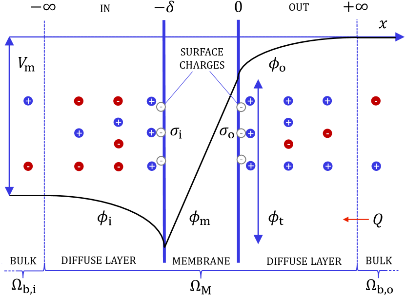
Figure 1: Profile of the electric potential across the cell membrane and the diffuse layers on each side. The minus signs in white denote surface charges ($\sigma_{\mathrm{i}}$ inside and $\sigma_{\mathrm{o}}$ outside), while the charges in solution are drawn in blue and red. The dotted lines delimit thermodynamic domains (see Sec. II.2). At rest, the membrane holds a potential difference ($V_{\mathrm{m}}=-70$ mV). Upon excitation, cations cross the membrane through ion channels (not depicted here) and $V_{\mathrm{m}}$ jumps to positive values. Simultaneously, electrical energy is dissipated as heat ($Q<0$).

We assume that equilibration of diffuse layers with the bulk electrolytes is fast compared to the dynamics of the action potential (this is verified in Section VII.1), which allows us to describe the concentration of ions in the diffuse layers close to the membrane with the Boltzmann distribution

$$c_{\mathrm{i},j}(x) =c_{\mathrm{i},j}(b)\>\exp{\{-\frac{z_{j}\>F\>\phi_{\mathrm{i}}}{R\>T}\}},$$ (4)

$$c_{\mathrm{o},j}(x) =c_{\mathrm{o},j}(b)\>\exp{\{-\frac{z_{j}\>F\>(\phi_{\mathrm{o}}-V_{\mathrm{m}})}{R\>T}\}},$$ (5)

where $c_{\mathrm{i},j}$ and $c_{\mathrm{o},j}$ are the concentrations of species $j$ inside and outside, respectively, and $RT/F$ is the thermal voltage ($RT/F=23.5$ mV at $T=273$ K). Applying Poisson’s equation to each compartment gives

$$\frac{d^{2}{\phi_{\mathrm{i}}}}{dx^{2}} =-\frac{\rho_{\mathrm{i}}}{\varepsilon},$$ (6)

$$\frac{d^{2}{\phi_{\mathrm{m}}}}{dx^{2}} =0,$$ (7)

$$\frac{d^{2}{\phi_{\mathrm{o}}}}{dx^{2}} =-\frac{\rho_{\mathrm{o}}}{\varepsilon},$$ (8)

where $\rho$ is the density of free charges (C m^-3), and $\varepsilon$ the dielectric permittivity of the internal and external solutions (water). Note that we assume that the free charge density is zero inside the membrane ($\rho_{\mathrm{m}}=0$), with a zero ion concentration inside the membrane. As $\rho_{\mathrm{i}}=\sum{z_{j}\>F\>c_{\mathrm{i},j}}$ and $\rho_{\mathrm{o}}=\sum{z_{j}\>F\>c_{\mathrm{o},j}}$, we obtain the following Poisson-Boltzmann equations:

$$\frac{d^{2}\phi_{\mathrm{i}}}{dx^{2}}(x) =-\frac{F}{\varepsilon}\sum^{N}_{j}\>z_{j}\>c_{\mathrm{i},j}(b)\>\exp{\{-\frac{z_{j}F\>\phi_{\mathrm{i}}(x)}{R\>T}\}},$$ (9)

$$\frac{d^{2}\phi_{\mathrm{o}}}{dx^{2}}(x) =-\frac{F}{\varepsilon}\sum^{N}_{j}\>z_{j}\>c_{\mathrm{o},j}(b)\>\exp{\{-\frac{z_{j}F\>[\phi_{\mathrm{o}}(x)-V_{\mathrm{m}}]}{R\>T}\}},$$ (10)

which we solve numerically, using boundary conditions given by Maxwell’s equations at an interface (Eqs. (15) and (16)). We now report the electrostatic relations necessary to derive energy changes in following sections. At rest, the membrane acts as a dielectric medium (ion channels are closed), storing a capacitive charge that we define as $-q$ in the internal solution and $+q$ in the external solution. In each compartment, this capacitive charge can be expressed as the sum of the charge that counter-balances the charges that belong to the surface of the membrane (that is $-\sigma_{\mathrm{i}}$ inside and $-\sigma_{\mathrm{o}}$ outside, both with units C m^-2) and the total mobile charge in solution, which we obtain by integrating the free charge density over the diffuse layers:

$$-q =\sigma_{\mathrm{i}}+\int_{-\infty}^{-\delta}{\rho_{\mathrm{i}}}\>dx,$$ (11)

$$q =\sigma_{\mathrm{o}}+\int_{0}^{\infty}{\rho_{\mathrm{o}}}\>dx.$$ (12)

Applying Poisson’s equation to the integrals above, we can relate the slope of the membrane potential at each interface to the total charge density in the internal and external solutions

$$\frac{d\phi_{\mathrm{i}}}{dx}(-\delta) =\frac{1}{\varepsilon}(\sigma_{\mathrm{i}}+q),$$ (13)

$$\frac{d\phi_{\mathrm{o}}}{dx}(0) =-\frac{1}{\varepsilon}\>\Big{(}\sigma_{\mathrm{o}}-q\Big{)},$$ (14)

Boundary conditions for electric potential at the two membrane-solution interfaces are given by

$$\varepsilon\frac{d\phi_{\mathrm{i}}}{dx}(-\delta)-\varepsilon_{\mathrm{m}}\frac{d\phi_{\mathrm{m}}}{dx}(-\delta) =\sigma_{\mathrm{i}},$$ (15)

$$\varepsilon_{\mathrm{m}}\frac{d\phi_{\mathrm{m}}}{dx}(0)-\varepsilon\frac{d\phi_{\mathrm{o}}}{dx}(0) =\sigma_{\mathrm{o}},$$ (16)

where $\varepsilon_{\mathrm{m}}$ is the dielectric permittivity of the membrane (F m^-1). By substituting Eq. (13) into (15), and Eq. (14) into (16) we can deduce that

$$\frac{q}{\varepsilon_{\mathrm{m}}}=\frac{d\phi_{\mathrm{m}}}{dx}(-\delta)=\frac{d\phi_{\mathrm{m}}}{dx}(0).$$ (17)

As the electric field is assumed to be constant inside the membrane, Eq. (17) gives

$$\frac{q}{\varepsilon_{\mathrm{m}}}=\frac{\phi_{\mathrm{m}}(0)-\phi_{\mathrm{m}}(-\delta)}{\delta}\overset{\Delta}{=}-\frac{\phi_{\mathrm{t}}}{\delta}.$$ (18)

We finally obtain an expression that relates the capacitive charge to the membrane’s capacitance ($c_{\mathrm{m}}$, in F m^-2) and the transmembrane potential:

$$q=-\frac{\varepsilon_{\mathrm{m}}}{\delta}\>\phi_{\mathrm{t}}=-c_{\mathrm{m}}\>\phi_{\mathrm{t}},$$ (19)

with $c_{\mathrm{m}}\overset{\Delta}{=}{\varepsilon_{\mathrm{m}}}/{\delta}$, identical to the result from Genet et al. (2000).

II.2 Thermodynamic definitions

To relate electrical energy changes at the membrane level to the exchange of heat with the surroundings, we need to define the membrane as a thermodynamic system. We divide the space into three domains (see Fig. 1): $\Omega_{\mathrm{M}}$ is the “membrane domain”, i.e. the region comprised of the membrane and the diffuse layers that form in the internal and external solutions, while $\Omega_{\mathrm{b,i}}$ and $\Omega_{\mathrm{b,o}}$ denote the internal and external bulk solutions, respectively. The first law of thermodynamics, $\Delta{U_{\mathrm{el}}}=Q+W_{\mathrm{el}}$, applies, in which $\Delta{U_{\mathrm{el}}}$ is the internal energy change associated with the variation of the membrane potential from $V_{\mathrm{m},0}$ to $V_{\mathrm{m}}$, $Q$ is the heat added to $\Omega_{\mathrm{M}}$ ($Q<0$ when heat is dissipated) and $W_{\mathrm{el}}$ is the electrical work done on $\Omega_{\mathrm{M}}$ by the surroundings. Since the capacitive charges $+q$ and $-q$ are confined to the diffuse layers close to the membrane (the bulk solutions are electroneutral), no electrical work is done on $\Omega_{\mathrm{M}}$ by the surrounding domains $\Omega_{\mathrm{b,i}}$ and $\Omega_{\mathrm{b,o}}$. The first law thus becomes

$$\Delta{U_{\mathrm{el}}}=Q.$$ (20)

The internal energy of the membrane system can be expressed as a sum of free energy and entropy-related energy:

$$\Delta{U_{\mathrm{el}}}=\Delta{F_{\mathrm{el}}}+T\Delta{S_{\mathrm{el}}},$$ (21)

where $\Delta{F_{\mathrm{el}}}$ and $\Delta{S_{\mathrm{el}}}$ are respectively the free energy and entropy change with respect to the resting state ($V_{\mathrm{m}}=-70$ mV). Thus, based on the aforementioned definitions, heat will be released ($Q<0$) from the membrane domain $\Omega_{\mathrm{M}}$ to the surroundings, as the (electric) internal energy of the membrane domain decreases ($\Delta{U_{\mathrm{el}}}<0$). In the following sections, we will derive the free energy and entropy changes in the membrane domain as a function of the membrane potentials $V_{\mathrm{m}}$ and $\phi_{\mathrm{t}}$. The sum of these energies will give the internal energy change (by Eq. (21)) associated with the (de)polarization of the membrane and therefore the quantity of heat that is reversibly released from the membrane domain $\Omega_{\mathrm{M}}$.

II.3 Electric free energy

The electric free energy of a linear dielectric medium is equal to its field energy Overbeek (1990); Jackson (1999); Landau et al. (2013), that is, in one dimension

$$F_{{\mathrm{el}}}=\frac{1}{2}\int^{+\infty}_{-\infty}{E.D}\>dx,$$ (22)

where $F_{{\mathrm{el}}}$ is the electric free energy (J m^-2), $E$ the electric field (V m^-1) and $D=\varepsilon\>E$ the displacement field (C m^-2). Interestingly, the field energy can be equated with the amount of heat dissipated by ionic currents in an electric field, using Maxwell’s equation for Ampere’s law (this is shown in Section VII.3). Note that the field energy is often regarded as an internal energy ($U_{\mathrm{el}}$), however, this is only true in a primitive model that considers the medium as structureless Frohlich (1968); Overbeek (1990). In a more refined model that takes into the effect of the electric field on the entropy of the dielectric medium (see SectionII.4), the field energy must be regarded as a free energy ($F_{\mathrm{el}}$) Frohlich (1968); Overbeek (1990). Applying Eq. (22) to the $\Omega_{\mathrm{M}}$ domain, we obtain the electric free energy as a function of the membrane potential $V_{\mathrm{m}}$. We obtain a free energy contribution from the double layers, which is

$$\begin{split}{F}^{\mathrm{DL}}_{\mathrm{el}}=&\frac{1}{2}\bigg{(}\int_{-\infty}^{-\delta}{\rho_{\mathrm{i}}(\phi_{\mathrm{i}}-V_{\mathrm{m}})}dx+\sigma_{\mathrm{i}}\>(\phi_{\mathrm{i}}(-\delta)-V_{\mathrm{m}})\\ &+\int^{+\infty}_{0}{\rho_{\mathrm{o}}\>\phi_{\mathrm{o}}\>}dx+\sigma_{\mathrm{o}}\>\phi_{\mathrm{o}}(0)\bigg{)},\end{split}$$ (23)

and one from the membrane capacitance, which is

$${F}^{\mathrm{m}}_{\mathrm{el}}=\frac{1}{2}\>c_{\mathrm{m}}\>\phi_{\mathrm{t}}\>V_{\mathrm{m}},$$ (24)

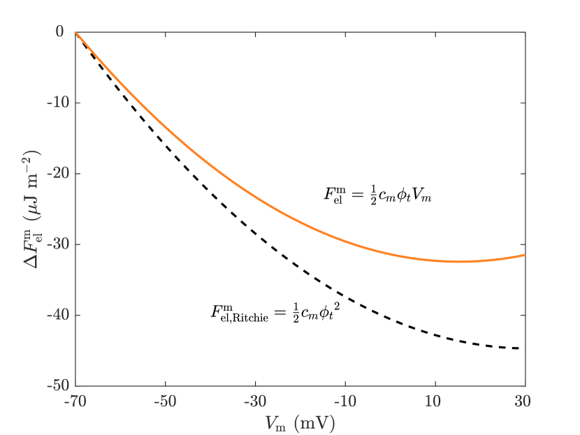
Figure 6: Free energy changes in the membrane, according to the revised Condenser Theory (this work, $\Delta F^{\mathrm{m}}_{\mathrm{el}}$ ) and to the formula suggested by Howarth et al. (1979) and Ritchie and Keynes (1985) ($\Delta F^{\mathrm{m}}_{\mathrm{el,Ritchie}}$ ). Strikingly, the latter overestimates free energy changes. Surface charge densities assumed are $\sigma_{\mathrm{i}}=-0.1$ C m^-2 and $\sigma_{\mathrm{o}}=-0.05$ C m^-2.

with ${F}_{\mathrm{el}}={F}^{\mathrm{DL}}_{\mathrm{el}}+{F}^{\mathrm{m}}_{\mathrm{el}}$. The first and third terms in Eq. (23) correspond to the energy of bulk charges in the diffuse layers of internal and external solutions and the second and fourth to the energy of the surface charges fixed onto the membrane. As shown by Eq. (24), the free energy contribution of the membrane capacitance is ${1}/{2}\>c_{\mathrm{m}}\>\phi_{\mathrm{t}}\>V_{\mathrm{m}}$, and not ${1}/{2}c_{\mathrm{m}}\>\phi_{\mathrm{t}}^{2}$ as proposed in Refs. Howarth et al. (1979) and Ritchie and Keynes (1985). The latter overestimates free energy changes, as compared to Eq. (24), see Fig. 6 in Section VII.6. The full derivation of Eqs. (23) and (24) is presented Section VII.4.

Finally, we write the free energy changes associated with the depolarisation of the membrane as $\Delta{F^{\mathrm{DL}}_{\mathrm{el}}}={F^{\mathrm{DL}}_{\mathrm{el}}}-{F^{\mathrm{DL}}_{\mathrm{el,0}}}$ and $\Delta{F^{\mathrm{m}}_{\mathrm{el}}}={F^{\mathrm{m}}_{\mathrm{el}}}-{F^{\mathrm{m}}_{\mathrm{el,0}}}$, where subscripts “0” mark the free energies calculated at the resting membrane potential, $V_{\mathrm{m,0}}=-70$ mV.

II.4 Entropy associated with the electric field

We consider two entropy terms: entropy changes associated with the polarization of water in the diffuse layers and entropy changes in the membrane.

II.4.1 In the diffuse layers

The electric field orders water dipoles in the diffuse layers, which decreases entropy. The change of entropy associated with the alignment of dipoles in a dielectric medium (water in our case) is related to the electric free energy by Frohlich (1968):

$$T\Delta{S}^{\mathrm{DL}}_{\mathrm{el}}=\frac{T}{\varepsilon}\frac{\partial{\varepsilon}}{\partial{T}}\Delta{F^{\mathrm{DL}}_{\mathrm{el}}}$$ (25)

where $\varepsilon$ is the dielectric permittivity of the medium. The value of ${T}/{\varepsilon}\>{\partial{\varepsilon}}/{\partial{T}}$ for water is -1.17 at 0°C and -1.4 at human body temperature (37°C) Floriano and Nascimento (2004); Lide (2004).

II.4.2 In the membrane

Similarly, entropy changes inside the lipid membrane have been proposed based on the temperature dependence of the membrane capacitance Howarth and Ritchie (1968); Howarth et al. (1979); Ritchie and Keynes (1985):

$$T\Delta{S^{\mathrm{m}}_{\mathrm{el}}}=\frac{T}{c_{\mathrm{m}}}\>\frac{\partial{c_{\mathrm{m}}}}{\partial{T}}\>\Delta{F^{\mathrm{m}}_{\mathrm{el}}}.$$ (26)

To verify that Eq. (26) holds, we adapted the derivation of Eq. (25), in which entropy is a function of ${\partial{\varepsilon}}/{\partial{T}}$, to the case in which entropy is a function of ${\partial{c_{\mathrm{m}}}}/{\partial{T}}$, the temperature dependence of the membrane capacitance. As shown in Section VII.5, Eq. (26) holds, under the assumption that the membrane capacitance has a linear dependence on temperature, but is constant with potential. Interestingly, it appears from recent experiments that the temperature dependence of the membrane capacitance arises from the variation of the lipid bilayer’s dimensions (thickness, $\delta$, and area, $A$, per lipid molecule) with temperature, rather than from the one of its dielectric permittivity (${\partial{\varepsilon_{\mathrm{m}}}}/{\partial{T}}\simeq 0$) Plaksin et al. (2018); Norbert Kucerka and Katsaras (2011); Szekely et al. (2011); Pan et al. (2008):

$$\frac{\partial{c_{\mathrm{m}}}}{\partial{T}}=\frac{\partial{(\varepsilon_{\mathrm{m}}\>A/\delta)}}{\partial{T}}\simeq\varepsilon_{\mathrm{m}}\frac{\partial{(A/\delta)}}{\partial{T}}.$$ (27)

Based on recent measurements of these dimensional changes Norbert Kucerka and Katsaras (2011); Szekely et al. (2011); Pan et al. (2008) Plaksin et al. (2018) have pointed out that the temperature dependence of the membrane capacitance remains close to $+0.3\%$/°C across several cellular types and artificial lipid membranes, suggesting that the rate of thermal response of the membrane is universal.

II.5 Parameters

Two important parameters in this model are the surface charge density on the interior ($\sigma_{\mathrm{i}}$ ) and exterior ($\sigma_{\mathrm{o}}$) sides of the membrane. Here we report ranges of values found in literature and then choose baselines for these two parameters. Hille (2001) compiled experimental data on excitable membranes, showing that the surface charge density (extracellular and intracellular) varies from $-0.04$ to $-0.16$ C m^-2. Other estimates give a wider range of values, from $-0.002$ to $-0.37$ C m^-2 Lakshminarayanaiah and Murayama (1975). In this work, the external surface charge density will be fixed to $\sigma_{\mathrm{o}}=-0.05$ C m^-2, and we will evaluate three cases for the internal surface charge density: $\sigma_{\mathrm{i}}=-0.05$, $-0.1$ and $-0.15$ C m^-2. There are several lines of evidence suggesting that neurons have more negative surface charges on the internal side of the membrane than on the external one. In rat cortical neurons for instance, Plaksin et al. (2018) estimated this surface charge bias to be $\sigma_{\mathrm{i}}-\sigma_{\mathrm{o}}=-0.1$ C m^-2. Further support for this hypothesis arises from the uneven distribution of phospholipids between the two sides of the membrane. In particular, phosphatidylserine, the most abundant negatively charged phospholipid in cell membranes, is found exclusively on the internal side of the cell membrane of neurons, where it has key signaling functions Kim et al. (2014). Other parameters used in the model are reported in Table 1.

Parameter	Value	Unit	Source
$\delta$	3	nm	Genet et al. (2000)
$c_{\mathrm{m}}$	9	mF m-2	Genet et al. (2000)
$V_{\mathrm{m}}$	-70	mV	Weiss (1996); Hille (2001); Genet et al. (2000)
${1}/{\varepsilon}\>{\partial{\varepsilon}}/{\partial{T}}$	- 0.43 at 0°C	$\%$K-1	Floriano and Nascimento (2004); Lide (2004)
${1}/{c_{\mathrm{m}}}\>{\partial{c_{\mathrm{m}}}}/{\partial{T}}$	+ 0.3	$\%$K-1	Plaksin et al. (2018)
$c_{\ce{Na+}}$	5 / 145	mM	Johnston and Wu (1994)
$c_{\ce{K+}}$	140 / 5	mM	Johnston and Wu (1994)
$c_{\ce{Ca^{2}+}}$	0.0001 / 2.5	mM	Johnston and Wu (1994)
$c_{\ce{Cl-}}$	145 / 155	mM	Johnston and Wu (1994)
$T$	273	K	Howarth et al. (1979)

Table 1: Parameters used in the electrostatic model and energy calculations. Concentrations are given in the format: internal solution / external solution.

III Results

III.1 Free energy changes

The change in electric free energy with membrane potential is depicted in Fig. 2, in the membrane ($\Delta{F^{\mathrm{m}}_{\mathrm{el}}}$) and in diffuse layers ($\Delta{F^{\mathrm{DL}}_{\mathrm{el}}}$), with and without surface charges on the membrane. First, when there are no surface charges, the free energy follows a parabola centred around $V_{\mathrm{m}}$ = 0 mV. The diffuse layers bring a relatively negligible contribution to the free energy in this case. Interestingly, the presence of an equal amount of surface charges on each side of the membrane ($\sigma_{\mathrm{i}}=\sigma_{\mathrm{o}}=-0.05$ C m^-2) results in almost no alteration of the energy changes as compared to the zero surface charge case. However, as more surface charges are present on the internal side than on the external side of the membrane ($\sigma_{\mathrm{i}}=2\>\sigma_{\mathrm{o}}$ and $3\>\sigma_{\mathrm{o}}$ ), both $\Delta{F^{\mathrm{m}}_{\mathrm{el}}}$ and $\Delta{F^{\mathrm{DL}}_{\mathrm{el}}}$ follow a steeper decrease, such that more free energy is released with increasing $V_{\mathrm{m}}$.

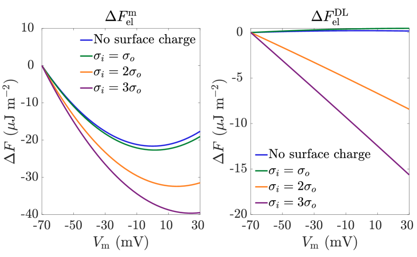
Figure 2: Change in electric free energy in the membrane ($\Delta{F}^{\mathrm{m}}_{\mathrm{el}}$) and in diffuse layers ($\Delta{F}^{\mathrm{DL}}_{\mathrm{el}}$) as a function of membrane potential, for an equal amount of surface charges ($\sigma_{\mathrm{i}}=\sigma_{\mathrm{o}}=-0.05$ C m^-2) and with a surface charge bias ($\sigma_{\mathrm{i}}=2\>\sigma_{\mathrm{o}}$ and $3\>\sigma_{\mathrm{o}}$). When a surface charge bias is present, more free energy is released, both in the membrane and diffuse layers.

III.2 Entropy changes

Entropy changes, depicted in Fig. 3, are proportional to the free energy changes presented above (by Eqs. (25) and (26)). As the membrane depolarizes (increasing $V_{\mathrm{m}}$), the entropy in the membrane ($T\Delta{S}^{\mathrm{m}}_{\mathrm{el}}$) decreases, while the one in diffuse layers ($T\Delta{S}^{\mathrm{DL}}_{\mathrm{el}}$) increases. Both entropy changes follow the same trend with surface charge distribution as the free energy changes in Fig. 2.

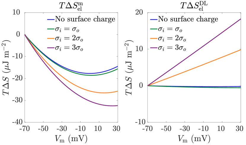
Figure 3: Entropy changes in the membrane ($T\Delta{S}^{\mathrm{m}}_{\mathrm{el}}$) and diffuse layers ($T\Delta{S}^{\mathrm{DL}}_{\mathrm{el}}$) with no surface charges, an equal amount of surface charges ($\sigma_{\mathrm{i}}=\sigma_{\mathrm{o}}=$-0.05 C m^-2) and with a surface charge bias ($\sigma_{\mathrm{i}}=2\>\sigma_{\mathrm{o}}$ and $3\>\sigma_{\mathrm{o}}$). The presence of a surface charge bias makes the entropy in the membrane decrease more upon depolarization, whereas it makes the entropy in diffuse layers increase.

III.3 Internal energy change, heat production and temperature change

The internal energy change occurring inside the $\Omega_{\mathrm{M}}$ domain, i.e the sum of the free and the entropic energy changes, is depicted in Fig. 4 according to the different scenarios of surface charge distribution used until now. The internal energy change provides a direct measure of the heat produced and absorbed by the nerve during the course of the action potential (Eq. (20)): an internal energy decrease ($\Delta{U}<0$) corresponds to a release of heat by the membrane domain ($Q<0$), whereas an internal energy increase ($\Delta{U}>0$) corresponds to an absorption of heat by the membrane domain ($Q>0$). An idealized action potential (modelled with a normal distribution function, for simplicity) and the corresponding heat profile are depicted in Fig. 5. We find that the presence of negative surface charges on the membrane leads to a more important decrease in internal energy (Fig. 4) and thus heat production (Fig. 5), especially when the membrane holds more fixed charges on its inside than outside. Interestingly, the bottom curve in Fig. 4 shows that when surface charges are distributed unevenly, the internal energy must not rise immediately after that $V_{\mathrm{m}}$ takes positive values. In other words, the membrane can release heat even when the membrane potential overshoots to positive values. This is reflected in Fig. 5 by the progressive disappearance of the “notch” in the energy profiles as $\sigma_{\mathrm{i}}$ becomes more negative than $\sigma_{\mathrm{o}}$.

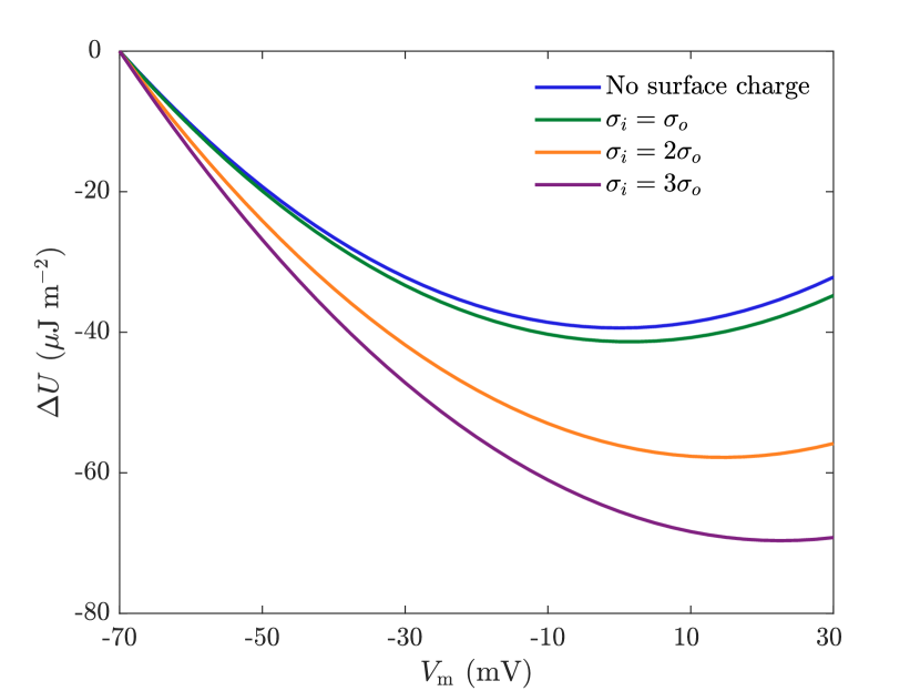
Figure 4: Internal energy changes of the membrane system, from top to bottom: without surface charge ($\sigma_{\mathrm{i}}=\sigma_{\mathrm{o}}=$ 0), with an equal amount of surface charges ($\sigma_{\mathrm{i}}=\sigma_{\mathrm{o}}=-0.05$ C m^-2), with a moderate surface charge bias ($\sigma_{\mathrm{i}}=2\>\sigma_{\mathrm{o}}$) and a bigger one ($\sigma_{\mathrm{i}}=3\>\sigma_{\mathrm{o}}$). The internal energy release increases with the presence of negative surface charges on each side of the membrane, and significantly more as the surface charge difference between the internal and external side of the membrane rises.

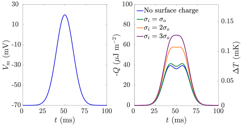
Figure 5: Left: an action potential depolarizes the membrane, starting from a resting potential of $V_{\mathrm{m}}$ = -70 mV at time 0, the membrane depolarizes to $V_{\mathrm{m}}$ = +20 mV at the peak of the action potential, before decreasing back to the resting potential. Right: concomitantly with the action potential, heat ($-Q$) is produced and absorbed, increasing the nerve temperature ($\Delta{T}$). See Section VII.2 for the calculation of temperature increase as a function of the heat released.

Finally, based on Fig. 5, we predict that a typical depolarization of the membrane from -70 mV to +20 mV Weiss (1996); Dudel et al. (2012) leads to a heat production of $-Q=40$ to $70\text{\,}\mathrm{\SIUnitSymbolMicro J}$ m^-2, depending on the magnitude of the bias of surface charges present on the membrane (0 to -0.1 C m^-2). If the action potential starts from a lower resting potential (which can be down to -100 mV Hille (2001)), up to $150\text{\,}\mathrm{\SIUnitSymbolMicro J}$ m^-2 of heat is predicted by the model. The predicted values fall in the range of experimental values (60 - $180\text{\,}\mathrm{\SIUnitSymbolMicro J}$ m^-2) Howarth et al. (1979)).

IV Discussion

The purpose of this work was to provide a theoretical background for heat production and absorption in neurons that goes beyond the simplistic analogy with a capacitor. Based on an equilibrium thermodynamics description of the membrane, its surface charges and double layers forming on each side, we evaluated the amount of heat released due to free energy and entropy changes during the action potential. The model assumes complete reversibility: all internal energy changes are first converted into heat, and then all heat is converted back to a change in the internal energy.

First, we found that the electric free energy of the cell membrane depends on both the membrane potential and the transmembrane potential, as shown by the new expression derived in this work: ${F}^{\mathrm{m}}_{\mathrm{el}}=\frac{1}{2}c_{\mathrm{m}}\>\phi_{\mathrm{t}}\>V_{\mathrm{m}}$. In consequence, the amount of free energy stored by the membrane increases as more surface charges are present on the internal versus the external side of the membrane. Free energy changes in the diffuse layers surrounding the membrane also increase significantly when a bias of surface charge is present, however, these changes are offset by the entropy changes associated with the polarization of water by the electric field, that are of comparable magnitude but of opposite sign ($\sim$-120% at 0°C). Finally, entropy changes in the membrane appear to be related to the dependence on temperature of the lipid bilayer’s dimensions rather than of its dielectric permittivity. Recent measurements of the dimensional variations allowed to determine that the magnitude of entropy changes is comparable ($\sim$+82$\%$) to the one of free energy changes.

The comparison of model predictions with the best-available measurements of the heat production and absorption in neurons supports the idea that the heat of nervous conduction has an electrical origin: assuming a typical action potential that depolarizes the membrane from -70 mV to +20 mV and a surface charge bias of $-0.05$ C m^-2 between the two sides of the membrane, we predict a production and absorption of heat of $\sim$60 $\text{\,}\mathrm{\SIUnitSymbolMicro J}$ m^-2, which is sufficient to reach the range of experimental values measured in the neurons of different organisms (60 - 180 $\text{\,}\mathrm{\SIUnitSymbolMicro J}$ m^-2) Howarth et al. (1979). Should the size of the action potential be larger (starting from a more negative resting potential), or the surface charge bias be more pronounced, more heat would be evolved.

Clearly, our predictions have a critical dependency on the action potential size and surface charge distribution between the internal and external sides of the membrane. Both parameters can vary from one type of neuron to the other, however, the values used for our calculations do not seem extravagant, considering the range of values reported in literature for surface charge density Hille (2001); Lakshminarayanaiah and Murayama (1975). The experimental validation of our predictions requires to compare the heat production with the true course of the action potential in neurons, which can only be obtained by measuring the membrane potential intracellularly. With the recent development of nano-electrodes Angle et al. (2015); Duan et al. (2013); Ferguson et al. (2012), there is hope that it is becoming possible to record true membrane potentials in the small neurons in which temperature changes can effectively be measured. Although we cannot discard the possibility of other sources of heat, such as heat arising from electrically-induced elastic displacements of the membrane El Hady and Machta (2015); Lacoste et al. (2009, 2007), our analysis suggests that the change in electrical energy of the membrane represents the most prominent mechanism of heat production and absorption by neurons during the propagation of the action potential.

Besides neurophysiology, the physics our work explores could be relevant for engineering electrical double layer capacitors Janssen and van Roij (2017) or designing capacitive deionization processes, which performance can be influenced by the presence of surface charges, either immobile Biesheuvel et al. (2015) or modulated electrochemically He et al. (2018). Moreover, thermodynamic analyses in capacitive systems typically do not include the entropy of dipoles in dielectric media Hemmatifar et al. (2018). Here, we showed that the entropy of dipoles brings a significant contribution to the internal energy stored across the double layers and the associated heat production and absorption.

V Author Information

Corresponding Authors: ^∗E-mail: bazant@mit.edu
Author Contributions:
^† A.D.L and J.P.D contributed equally to this work.

VI Acknowledgements

J.P.D. acknowledges support in the form of a National Science Foundation Graduate Research Fellowship under Grant No. 1122374. A.D.L. acknowledges support from the Louis-de-Broglie Foundation of the French Academy of Sciences. The authors thank Mathijs Janssen and Maarten Biesheuvel for useful comments.

VII Appendix

VII.1 Fast equilibration of double layers

In this work, we describe ions and the electric potential in the diffuse layers at equilibrium, with the Boltzmann distribution (Eqs. (9) and (10)). This equilibrium assumption decouples the problem from time dependence for relaxation of the double layers and simplifies it to a single dependence on the membrane potential $V_{\mathrm{m}}$. However, in reality, $V_{\mathrm{m}}$ is time-dependent. We must thus verify that the double layers reach their equilibrium conformation (ion concentration versus position) significantly faster than the variation of $V_{\mathrm{m}}$ during the course of the action potential. Two time scales can characterize the relaxation of diffuse layers: diffusion $\tau_{D}={L^{2}}/{D}$ and charge density relaxation $\tau_{L}={\lambda_{D}^{2}}/{D}$, where L is the characteristic length, D the characteristic diffusivity, and $\lambda_{D}$ the Debye length. At low voltages, Bazant et al. (2004) have shown that the primary time scale for diffuse charges dynamics in a non-Faradaic electrochemical cell is the harmonic mean between these time constants, that is: $\tau_{C}=\lambda_{D}\>L/D$. Interestingly, a recent study by Janssen (2019) has shown that the easily obtainable $\tau_{C}$ decently describes double layer relaxation also in cylindrical geometry, the relevant geometry for neurons. By analogy with the electrochemical cell, the membrane can be seen as sandwiched between two electrodes separated by a distance $L$, and on which a difference of potential is applied Lacoste et al. (2009); Ziebert and Lacoste (2011).
In physiological conditions (ionic strength = 150 mM) and at 0$\degree$C, the Debye length is less than 1 nm:

$$\lambda_{D}=\sqrt{\frac{RT\>\varepsilon}{F^{2}\sum{z_{j}^{2}\>c_{j}}}}=\>0.6\>\mathrm{nm}.$$ (28)

In the garfish olfactory nerve, one of the smallest axons studied, the characteristic length is given by the radius of the cell, $L/2=0.25$ $\text{\,}\mathrm{\SIUnitSymbolMicro m}$. Taking $D=10^{-9}$ m² $s^{-1}$ we find $\tau_{C}=0.3$ $\text{\,}\mathrm{\SIUnitSymbolMicro s}$. In the giant squid axon, one of the largest axons ever studied, we have $L/2=200$ $\text{\,}\mathrm{\SIUnitSymbolMicro m}$, and thus $\tau_{C}=240$ $\text{\,}\mathrm{\SIUnitSymbolMicro s}$. These characteristic times for relaxation are small compared to the time scale of compound action potentials, which is 10 to 100 ms Howarth et al. (1979). While in the nonlinear regime (where the double layer potential across each side is much larger than the thermal voltage $\sim$24 mV) the time scale for bulk salt diffusion $\tau_{D}=L^{2}/D$ can be important, the leading order dynamics occur at the $\tau_{C}$ scale. Therefore, we neglect any double layer relaxation effect and treat them at equilibrium.

VII.2 Fast equilibration of temperature inside the nerve

Another important assumption we make is the fast heat equilibration between the cell membrane and the rest of the nerve. The validity of this assumption can be verified based on scaling analysis on the heat equation, which yields a characteristic time for heat diffusion:

$$\tau_{\mathrm{h}}=\frac{\rho\>c_{\mathrm{p}}\>L^{2}}{K}$$ (29)

where $\rho$ is the mass density, $c_{\mathrm{p}}$ the specific heat capacity, $L$ the characteristic length and $K$ the thermal conductivity. With $L=0.125\>$\text{\,}\mathrm{\SIUnitSymbolMicro m}$$, $\rho=5.8$ g cm^-3, $c_{\mathrm{p}}=3.6$ J (g.K)^-1 Howarth et al. (1979), and using the thermal conductivity of water at 0$\degree$C, $K=0.0056$ J (K cm s)^-1 Weast et al. (1988), we find $\tau_{\mathrm{h}}\sim 0.6$ µs. Thus, the heat equilibration in the interior of the small nerve fibers in which the heat experiments were conducted Howarth et al. (1979) is on the order of microseconds, which is much quicker than the timescale of the action potential in these nerves (10 to 100 ms) Howarth et al. (1979). The nerve is solely composed of densely-packed fibers, such that the mean distance between fibers is smaller than the size of a single fiber Easton (1971). Thus, we assume that the whole nerve volume is at thermal equilibrium during the action potential, and calculate the rise of the nerve’s temperature as proportional to the amount of heat dissipated:

$$\Delta{T}=-\frac{\Delta{Q}}{c_{\mathrm{p}}}\>A_{\mathrm{m}},$$ (30)

where $A_{\mathrm{m}}=65000$ cm² g^-1 is the total membrane area per mass of nerve Howarth et al. (1979).

VII.3 The Condenser Theory from Maxwell’s equation for Ampere’s law

Heat production and field energy can be unified by Maxwell’s equation for Ampere’s law Jacobs (2013),

$$E\>(\nabla\times{H})=E\>{J}+E\>{\frac{\partial{D}}{\partial{t}}},$$ (31)

where $J$ is the current density (A m^-2), $H$ is the magnetic field and $D$ the displacement. -$E\>{J}$ is the energy dissipated by an ionic current $J$ in an electric field $E$ as heat per unit of volume and time Jacobs (2013), noted $\dot{Q}_{\mathrm{V}}$ (negative when heat is dissipated). Neglecting magnetic contributions, and in one dimension, we find

$$\dot{Q}_{\mathrm{V}}=-E\>J=E\>{\frac{\partial{D}}{\partial{t}}}.$$ (32)

This relationship offers another way to understand the Condenser Theory: during the action potential, positive charges (Na+ and K+ ions) move through ion channels of the membrane Hille (2001), first in the same direction as the electric field ($-E.J<0$, in one dimension), then against the electric field ($-E.J>0$), which results in heat production ($\dot{Q}_{\mathrm{V}}<0$) and then heat absorption ($\dot{Q}_{\mathrm{V}}>0$). Let’s consider the situation where the field is 0 at time zero and $E$ at time $t$. If the dielectric medium is linear ($D=\varepsilon.E$), the heat absorbed between time $0$ and $t$ is equal to the field energy at time $t$:

$$\begin{split}Q_{\mathrm{V}}&=\int_{0}^{t}{E\>{\frac{\partial{D}}{\partial{t}}}}\>dt=\frac{1}{2}\int_{0}^{t}{\Big{(}E\>{\frac{\partial{D}}{\partial{t}}}+\frac{\partial{E}}{\partial{t}}\>{D}\Big{)}}\>dt\\ &=\frac{1}{2}E\>{D}.\end{split}$$ (33)

The second equality holds for any linear dielectric medium, whereas the third is given by the fundamental theorem of calculus. Finally, integrating $Q_{\mathrm{V}}$ over the membrane domain $\Omega_{\mathrm{M}}$ gives the heat dissipated per unit of membrane surface area (J/m²):

$$Q=\int^{+\infty}_{-\infty}{\int_{0}^{t}{E\>{\frac{\partial{D}}{\partial{t}}}}\>dt\>dx=\int^{+\infty}_{-\infty}\frac{1}{2}E\>D}\>dx.$$ (34)

This last expression gives the amount of heat that is dissipated upon release of the electric free energy of a dielectric medium Overbeek (1990); Jackson (1999).

VII.4 Derivation of the electric free energy of the membrane capacitance and of double layers

In this section we split the free energy of the $\Omega_{\mathrm{M}}$ domain (given by Eq. (22) or (34)) into a contribution from the membrane capacitance and one form the double layers. This separation is necessary to entropy calculations (Section II.4). We start by expanding the field energy expression over the internal diffuse layer, the membrane, and the external diffuse layer:

$$\begin{split}F_{\mathrm{el}}=&\frac{1}{2}\bigg{[}\varepsilon\int_{-\infty}^{-\delta}{\bigg{(}\frac{d{\phi_{\mathrm{i}}(x)}}{d{x}}}\bigg{)}^{2}dx+\varepsilon_{\mathrm{m}}\int_{-\delta}^{0}{\bigg{(}\frac{d{\phi_{\mathrm{m}}(x)}}{d{x}}}\bigg{)}^{2}dx\\ &+\varepsilon\int_{0}^{+\infty}{\bigg{(}\frac{d{\phi_{\mathrm{o}}(x)}}{d{x}}}\bigg{)}^{2}dx\bigg{]}.\\ \end{split}$$ (35)

Assuming the density of free charges to be zero at any point $]-\delta;0[$ inside the membrane, Poisson’s equation requires the field to be constant across the membrane, such that $\frac{d{\phi_{\mathrm{m}}(x)}}{d{x}}$ = $\frac{d{\phi_{\mathrm{m}}(0)}}{d{x}}$. The second term in the RHS of Eq. (35), then simplifies to

$$\begin{split}\varepsilon_{\mathrm{m}}\int_{-\delta}^{0}\bigg{(}\frac{d{\phi_{\mathrm{m}}(x)}}{d{x}}\bigg{)}^{2}dx&=\varepsilon_{\mathrm{m}}\int_{-\delta}^{0}\bigg{(}\frac{d\phi_{\mathrm{m}}(0)}{dx}\bigg{)}^{2}dx\\ &=\varepsilon_{\mathrm{m}}\bigg{(}\frac{q}{\varepsilon_{\mathrm{m}}}\bigg{)}^{2}\int_{-\delta}^{0}{}dx\\ &=\frac{q^{2}}{c_{\mathrm{m}}}.\\ \end{split}$$ (36)

The second equality is given by boundary conditions for the electric field, Eq. (17). Next, integration by parts of the first and third terms in Eq. (35) gives

$$\begin{split}F_{\mathrm{el}}=&\frac{1}{2}\bigg{(}\varepsilon\>\left[{\frac{d{\phi_{\mathrm{i}}}}{d{x}}\>\phi_{\mathrm{i}}}\right]^{-\delta}_{-\infty}-\varepsilon\int_{-\infty}^{-\delta}{\phi_{\mathrm{i}}\>\frac{d^{2}{\phi_{\mathrm{i}}}}{d{x^{2}}}}dx+\frac{q^{2}}{c_{\mathrm{m}}}\\ &+\varepsilon\>\left[{\frac{d{\phi_{\mathrm{o}}}}{d{x}}\>\phi_{\mathrm{o}}}\right]^{+\infty}_{0}-\varepsilon\int^{+\infty}_{0}{\phi_{\mathrm{o}}\>\frac{d^{2}{\phi_{\mathrm{o}}}}{d{x^{2}}}}dx\bigg{)}.\end{split}$$ (37)

Remembering that the potential is constant at $-\infty$ and $+\infty$, using Eqs. (13) and (14) and Poisson’s equation, Eq. (37) can be rearranged into

$$\begin{split}F_{\mathrm{el}}=&\frac{1}{2}\bigg{(}\int_{-\infty}^{-\delta}{\rho_{\mathrm{i}}\>\phi_{\mathrm{i}}\>}dx+\Big{(}\sigma_{\mathrm{i}}+q\Big{)}\>\phi_{\mathrm{i}}(-\delta)\\ &+\int^{+\infty}_{0}{\rho_{\mathrm{o}}\>\phi_{\mathrm{o}}\>}dx+\Big{(}\sigma_{\mathrm{o}}-q\Big{)}\>\phi_{\mathrm{o}}(0)+\frac{q^{2}}{c_{\mathrm{m}}}\bigg{)}.\\ \end{split}$$ (38)

As $q=-c_{\mathrm{m}}(\phi_{\mathrm{i}}(-\delta)-\phi_{\mathrm{o}}(0))$ by Eq. (19), this last expression simplifies to

$$\begin{split}F_{\mathrm{el}}=&\frac{1}{2}\bigg{(}\int_{-\infty}^{-\delta}{\rho_{\mathrm{i}}\>\phi_{\mathrm{i}}\>}dx+\sigma_{\mathrm{i}}\>\phi_{\mathrm{i}}(-\delta)\\ &+\int^{+\infty}_{0}{\rho_{\mathrm{o}}\>\phi_{\mathrm{o}}\>}dx+\sigma_{\mathrm{o}}\>\phi_{\mathrm{o}}(0)\bigg{)}.\end{split}$$ (39)

By applying the substitution $\phi_{\mathrm{i}}=(\phi_{\mathrm{i}}-V_{\mathrm{m}})+V_{\mathrm{m}}$ and using Eqs. (11) and (19), we separate the free energy in the diffuse layers $(F^{\mathrm{DL}}_{\mathrm{el}})$ from the one in the membrane $(F^{\mathrm{m}}_{\mathrm{el}})$:

$$\begin{split}F^{\mathrm{DL}}_{\mathrm{el}}=&\frac{1}{2}\bigg{(}\int_{-\infty}^{-\delta}{\rho_{\mathrm{i}}(\phi_{\mathrm{i}}-V_{\mathrm{m}})}dx+\sigma_{\mathrm{i}}\>(\phi_{\mathrm{i}}(-\delta)-V_{\mathrm{m}})\\ &+\int^{+\infty}_{0}{\rho_{\mathrm{o}}\>\phi_{\mathrm{o}}\>}dx+\sigma_{\mathrm{o}}\>\phi_{\mathrm{o}}(0)\bigg{)},\end{split}$$ (40)

and

$$F^{\mathrm{m}}_{\mathrm{el}}=\frac{1}{2}\>c_{\mathrm{m}}\>\phi_{\mathrm{t}}\>V_{\mathrm{m}},$$ (41)

with $F_{\mathrm{el}}=F^{\mathrm{DL}}_{\mathrm{el}}+F^{\mathrm{m}}_{\mathrm{el}}$.

VII.5 Derivation of entropy changes in the membrane

Within the Condenser Theory, it was suggested that entropy changes in the lipid bilayer accompanying the action potential could account for up to 4 times the free energy changes Howarth et al. (1979); Ritchie (1973). The ratio between the entropy-related energy and the free energy was calculated as

$$\frac{T\Delta{S}}{\Delta{F}}=\frac{T}{C}\>\frac{\partial{C}}{\partial{T}}$$ (42)

where $C$ is the membrane capacitance. However, no full derivation of this equation is reported in the literature. Here we will show under which conditions Eq. 42 can be derived, based on the demonstration Frohlich (1968). For simplicity, we will consider a membrane without any surface charges, holding a charge $q$ on each side (here $q$ is the capacitive charge in C), across a potential difference $V$. This simplification will ease notations without modifying the relation between the membrane’s entropy and electric free energy studied here. We start by considering the change of internal energy $dU$ (in J) following an increment of charge $dq$. The first law of thermodynamics reads

$$dU =dQ+dW$$

$$=dQ+V\>dq$$

where $dQ$ is the influx of heat and $dW$ is the electrical work done on the membrane. Note that the electrical work did not appear explicitly in the thermodynamic system defined in Section II.2, since no electrical work is done on $\Omega_{\mathrm{M}}$ by the surroundings (the latter is however implicitly accounted for as $\Delta{F_{\mathrm{el}}}$ in Eq. 21). For the purpose of this demonstration, the thermodynamic system considered here consists of the membrane only ($x\>\epsilon\>]-\delta;0[$), which enables us to express the electrical work associated with the depolarization and repolarization of the membrane explicitly. Assuming that the capacitance $C$ remains constant with $V$ but depends on the temperature $T$, we obtain

$$dq=d(C.V)=dC.V+C.dV=\frac{\partial{C}}{\partial{T}}\>dT.V+C.d(V).$$ (43)

Thus, a variation of $q$ may be due to a variation of temperature or of potential, the capacitance being assumed to remain constant for the range of physiological potentials ($ca.$ - 100 mV to + 20 mV). By taking $T$ and $V^{2}$ as independent variables, the first law now becomes

$$dQ+V^{2}\frac{\partial{C}}{\partial{T}}\>dT+\frac{1}{2}C\>d(V^{2})=dU=\frac{\partial{U}}{\partial{T}}\>dT+\frac{\partial{U}}{\partial{(V^{2})}}\>d(V^{2}).$$ (44)

Note that $dQ$ is not a total differential, however $dS=dQ/T$ is one, for a reversible process Jackson (1999). This property means that a unique function $S(T,V^{2})$ must exist, such that

$$dS=\frac{\partial{S}}{\partial{T}}\>dT+\frac{\partial{S}}{\partial{(V^{2})}}\>d(V^{2}).$$ (45)

Thus if there is a relation $dS=f(T,V^{2}).dT+g(T,V^{2}).dV^{2}$, where f and g are two unknown functions, the condition that $dS$ is a total differential requires that

$$\frac{\partial{f}}{\partial{(V^{2})}}=\frac{\partial{g}}{\partial{T}},$$ (46)

as both sides of Eq. 46 are equal to ${\partial^{2}{S}}/({\partial{T}\partial{(V^{2})}})$, by Eq. 45. Next, by substituting for $dS=dQ/T$ in Eq. (44), we find

$$dS=\frac{1}{T}\Big{(}\frac{\partial{U}}{\partial{T}}-V^{2}\frac{\partial{C}}{\partial{T}}\Big{)}dT+\frac{1}{T}\Big{(}\frac{\partial{U}}{\partial{(V^{2})}}-\frac{C}{2}\Big{)}d(V^{2}).$$ (47)

This equation is analogous to Eq. (45) and therefore, Eq. (46) becomes

$$\frac{\partial}{\partial{(V^{2})}}\Big{\{}\frac{1}{T}\Big{(}\frac{\partial{U}}{\partial{T}}-V^{2}\frac{\partial{C}}{\partial{T}}\Big{)}\Big{\}}=\frac{\partial}{\partial{T}}\Big{\{}\frac{1}{T}\Big{(}\frac{\partial{U}}{\partial{(V^{2})}}-\frac{C}{2}\Big{)}\Big{\}}.$$ (48)

By carrying out differentiations we find (take ${\partial{C}}/{\partial{T}}$ as a constant):

$$\frac{\partial{U}}{\partial{(V^{2})}}=\frac{C}{2}+\frac{1}{2}\frac{\partial{C}}{\partial{T}}T$$ (49)

Finally, upon integration, we obtain

$$\Delta{U}=\frac{1}{2}\int^{V^{2}}_{0}\Big{(}C+\frac{\partial{C}}{\partial{T}}T\Big{)}d(V^{2})=\frac{1}{2}CV^{2}+\frac{1}{2}\frac{\partial{C}}{\partial{T}}T\>V^{2}.$$ (50)

The first term is the free energy change $\Delta{F}$ of the capacitor, whereas the second is the energy associated with a change of entropy $T\Delta{S}$. Thus we have

$$T\Delta{S}=\Delta{U}-\Delta{F}=\frac{1}{2}\frac{\partial{C}}{\partial{T}}T\>V^{2}=\frac{T}{C}\>\frac{\partial{C}}{\partial{T}}\Delta{F},$$ (51)

and Eq. (26) holds, under the condition that the membrane capacitance has a linear dependence on temperature, but is constant with potential. A number of recent studies indicate that there exists such a linear dependence and that the value of ${\partial{C}}/{\partial{T}}$ is $\sim 0.3\%/\degree$C for a wide range of cell membranes Plaksin et al. (2018); Carvalho-de Souza et al. (2015); Martino et al. (2015); Hotka and Zahradnik (2014); Shapiro et al. (2012). Why does the membrane capacitance change with temperature? Using the classical model for the membrane capacitance, $C=\varepsilon_{\mathrm{m}}\>{A}/{d}$, where $A$ is the membrane area, and $\delta$ the membrane thickness, the temperature dependence could be attributed to a variation of the dielectric permittivity ${\partial{\varepsilon_{\mathrm{m}}}}/{\partial{T}}$, or to a variation of the membrane dimensions (${\partial{A}}/{\partial{T}}$ and ${\partial{\delta}}/{\partial{T}}$). Dimensional changes have been measured in artificial lipid bilayers Pan et al. (2008); Norbert Kucerka and Katsaras (2011); Szekely et al. (2011), and in neurons, these changes correspond to a $0.11$+-$0.03\%$/K reduction in the lipid membrane thickness and a $0.22$+-$0.03\%/\degree$C increase in the area per lipid, resulting in a linear increase of the capacitance with temperature of 0.3 $\%$/K Plaksin et al. (2018). Little is known on how the membrane’s dielectric permittivity varies with temperature, however ${\partial{\varepsilon_{\mathrm{m}}}}/{\partial{T}}$ has been measured for unsaturated fatty acids (the molecules composing the core of the membrane), yielding values more than one order of magnitude smaller than the combined dimensional changes Plaksin et al. (2018); Lizhi et al. (2008).

VII.6 Supplementary plots

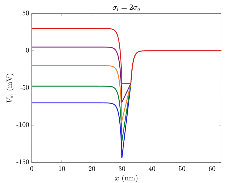
Figure 7: Profiles of the electric potential across the membrane and the surrounding diffuse layers, for different values of the membrane potential $V_{\mathrm{m}}$ (-70 to +30 mV). TOP: surface charge densities are equal on each side ($\sigma_{\mathrm{i}}=\sigma_{\mathrm{o}}=-0.05$ C m^-2). BOTTOM: a bias of surface charges makes the internal side more negative ($\sigma_{\mathrm{i}}=$-0.1 C m^-2 and $\sigma_{\mathrm{o}}=-0.05$ C m^-2), such that the transmembrane potential $\phi_{\mathrm{t}}$ need not to reverse when the membrane potential is positive (in purple).

References

- Hodgkin et al. (1952) A. L. Hodgkin, A. F. Huxley, and B. Katz, The Journal of physiology 116, 424 (1952).
- Hodgkin and Huxley (1952) A. L. Hodgkin and A. F. Huxley, The Journal of physiology 116, 473 (1952).
- Neher and Sakmann (1992) E. Neher and B. Sakmann, Scientific American 266, 44 (1992).
- Hamill et al. (1981) O. P. Hamill, A. Marty, E. Neher, B. Sakmann, and F. Sigworth, Pflügers Archiv 391, 85 (1981).
- Howarth et al. (1979) J. V. Howarth, J. M. Ritchie, and D. Stagg, Proc. R. Soc. Lond. 367, 347 (1979).
- Tasaki et al. (1968) I. Tasaki, A. Watanabe, R. Sandlin, and L. Carnay, Proceedings of the National Academy of Sciences 61, 883 (1968).
- Tasaki et al. (1989) I. Tasaki, K. Kusano, and P. M. Byrne, Biophysical Journal 55, 1033 (1989).
- Gonzalez-Perez et al. (2016) A. Gonzalez-Perez, L. D. Mosgaard, R. Budvytyte, E. Villagran-Vargas, A. D. Jackson, and T. Heimburg, Biophysical Chemistry 216, 51 (2016).
- Hille (2001) B. Hille, Ion channels of excitable membranes, Vol. 507 (Sinauer Sunderland, MA, 2001).
- El Hady and Machta (2015) A. El Hady and B. B. Machta, Nature Communications 6, 6697 (2015).
- Abbott et al. (1958) B. C. Abbott, A. V. Hill, and J. V. Howarth, Proceedings of the Royal Society B: Biological Sciences 148, 149 (1958).
- Howarth and Ritchie (1968) K. R. D. Howarth, J. and J. M. Ritchie, The Journal of Physiology , 745 (1968).
- Ritchie and Keynes (1985) J. M. Ritchie and R. D. Keynes, Quaterly Review of Biophysics 18, 451 (1985).
- Ritchie (1973) J. Ritchie, Progress in biophysics and molecular biology 26, 147 (1973).
- Easton (1971) D. M. Easton, Science 172, 952 (1971).
- Weiss (1996) T. F. Weiss, Cellular biophysics, Vol. 1 (MIT press Cambridge, Massachusetts, 1996).
- Taylor et al. (1962) R. Taylor, W. Chandler, and W. Knox, Biophysical Society Abstracts (1962).
- Plaksin et al. (2018) M. Plaksin, E. Shapira, E. Kimmel, and S. Shoham, Physical Review X 8, 11043 (2018).
- Lizhi et al. (2008) H. Lizhi, K. Toyoda, and I. Ihara, Journal of Food Engineering 88, 151 (2008).
- Genet et al. (2000) S. Genet, R. Costalat, and J. Burger, Acta Biotheoretica 48, 273 (2000).
- Overbeek (1990) J. T. G. Overbeek, Colloids and Surfaces 51, 61 (1990).
- Jackson (1999) J. D. Jackson, Classical electrodynamics (AAPT, 1999).
- Landau et al. (2013) L. D. Landau, J. Bell, M. Kearsley, L. Pitaevskii, E. Lifshitz, and J. Sykes, Electrodynamics of continuous media, Vol. 8 (Elsevier, 2013).
- Frohlich (1968) H. Frohlich, Theory of Dielectrics: Dielectric Constant and Dielectric Loss, Monographs on the physics and chemistry of materials (Oxford University Press, 1968).
- Floriano and Nascimento (2004) W. B. Floriano and M. A. C. Nascimento, Brazilian Journal of Physics 34, 38 (2004).
- Lide (2004) D. R. Lide, CRC handbook of chemistry and physics, Vol. 85 (CRC press, 2004).
- Norbert Kucerka and Katsaras (2011) M.-P. N. Norbert Kucerka and J. Katsaras, Biochimica et Biophysica Acta (BBA) - Biomembranes 1808, 2761 (2011).
- Szekely et al. (2011) P. Szekely, T. Dvir, R. Asor, R. Resh, A. Steiner, O. Szekely, A. Ginsburg, J. Mosenkis, V. Guralnick, Y. Dan, et al., The Journal of Physical Chemistry B 115, 14501 (2011).
- Pan et al. (2008) J. Pan, S. Tristram-Nagle, N. Kucerka, and J. F. Nagle, Biophysical journal 94, 117 (2008).
- Lakshminarayanaiah and Murayama (1975) N. Lakshminarayanaiah and K. Murayama, Journal of Membrane Biology 23, 279 (1975).
- Kim et al. (2014) H.-Y. Kim, B. X. Huang, and A. A. Spector, Progress in lipid research 56, 1 (2014).
- Johnston and Wu (1994) D. Johnston and S. M.-S. Wu, Foundations of cellular neurophysiology (MIT press, 1994).
- Dudel et al. (2012) J. Dudel, W. Janig, and M. Zimmermann, Fundamentals of neurophysiology (Springer Science & Business Media, 2012).
- Angle et al. (2015) M. R. Angle, B. Cui, and N. A. Melosh, Current Opinion in Neurobiology 32, 132 (2015).
- Duan et al. (2013) X. Duan, T.-M. Fu, J. Liu, and C. M. Lieber, Nano Today 8, 351 (2013).
- Ferguson et al. (2012) J. E. Ferguson, C. Boldt, J. G. Puhl, T. W. Stigen, J. C. Jackson, K. M. Crisp, K. A. Mesce, T. I. Netoff, and A. D. Redish, Nanomedicine 7, 847 (2012).
- Lacoste et al. (2009) D. Lacoste, G. Menon, M. Bazant, and J. Joanny, The European Physical Journal E 28, 243 (2009).
- Lacoste et al. (2007) D. Lacoste, M. C. Lagomarsino, and J. Joanny, EPL (Europhysics Letters) 77, 18006 (2007).
- Janssen and van Roij (2017) M. Janssen and R. van Roij, Physical review letters 118, 096001 (2017).
- Biesheuvel et al. (2015) P. Biesheuvel, H. Hamelers, and M. Suss, Colloids and Interface Science Communications 9, 1 (2015).
- He et al. (2018) F. He, P. Biesheuvel, M. Z. Bazant, and T. A. Hatton, Water research 132, 282 (2018).
- Hemmatifar et al. (2018) A. Hemmatifar, A. Ramachandran, K. Liu, D. I. Oyarzun, M. Z. Bazant, and J. G. Santiago, Environmental science & technology 52, 10196 (2018).
- Bazant et al. (2004) M. Z. Bazant, K. Thornton, and A. Ajdari, Physical review E 70, 021056 (2004).
- Janssen (2019) M. Janssen, arXiv e-prints , arXiv:1907.06894 (2019), arXiv:1907.06894 [physics.chem-ph] .
- Ziebert and Lacoste (2011) F. Ziebert and D. Lacoste, in Advances in planar lipid bilayers and liposomes, Vol. 14 (Elsevier, 2011) pp. 63–95.
- Weast et al. (1988) R. C. Weast, M. J. Astle, W. H. Beyer, et al., CRC handbook of chemistry and physics, Vol. 69 (CRC press Boca Raton, FL, 1988).
- Jacobs (2013) P. Jacobs, Thermodynamics (World Scientific Publishing Company, 2013).
- Carvalho-de Souza et al. (2015) J. L. Carvalho-de Souza, J. S. Treger, B. Dang, S. B. Kent, D. R. Pepperberg, and F. Bezanilla, Neuron 86, 207 (2015).
- Martino et al. (2015) N. Martino, P. Feyen, M. Porro, C. Bossio, E. Zucchetti, D. Ghezzi, F. Benfenati, G. Lanzani, and M. R. Antognazza, Scientific reports 5, 8911 (2015).
- Hotka and Zahradnik (2014) M. Hotka and I. Zahradnik, Biophysical Journal 106, 121a (2014).
- Shapiro et al. (2012) M. G. Shapiro, K. Homma, S. Villarreal, C. P. Richter, and F. Bezanilla, Nature Communications 3, 310 (2012).